The split-ring Josephson resonator as an artificial atom

Abstract

Using the resistive-shunted-junction model we show that a split-ring Josephson oscillator or radio-frequency SQUID in the hysteretic regime is similar to an atomic system. It has a number of stationary states that we characterize. Applying a short magnetic pulse we switch the system from one state to another. These states can be detected via the reflection of a small amplitude signal forming the base of a new spectroscopy.

I Introduction

Since the realization of lasers using atoms in the sixties, many researchers have been trying to replicate this effect using quantum objects similar to two-level systems. The basic elements to realize a laser are encyclopedia_nl (i) energy levels for the electrons, (ii) a pumping mechanism to populate upper levels and (iii) an optical cavity to confine photons enhancing the probability of interacting with excited electrons. A Josephson junction between two superconductors is a macroscopic quantum system and Tilley tilley predicted that interconnected Josephson junctions could emit a coherent radiation. Rogovin and Sculley rs76 also established a connection between Josephson junctions and two-level quantum systems. The superradiance prediction was confirmed by Barbara et al bcsl99 who showed that the power emitted by an array grows like $N^{2}$ where $N$ is the number of active junctions in the array. See also the recent experiments by Ottaviani et al ocl09 showing the synchronization of junctions in an array. Since the radiation emitted is in the Terahertz range where there are no solid-state sources, these systems are being investigated as microwave sources (see for example ok07 ). Up to now however practical difficulties subsist and the powers emitted by such devices remain low.

From another point of view artificial materials (Metamaterials) have been fabricated by embedding metal split-rings or rods into dielectric materials. This way negative index materials have been fabricatedVeselago:06 , Pendry:04 . One can obtain artificial atoms with a high magnetic moment and a nonlinear response to electromagnetic waves. Such an artificial atom would have many advantages over a real atom. For atoms the dipole momentum is very small and the interactions between them are small. To realize interactions large density are necessary. Also in general the excited state has an energy much larger than the energy of the dipole coupled with electromagnetic wave. Many candidates for artificial atoms have been proposed, most of them width intrinsic nonlinearities. Among them we have a diode Lapin:2003 , a Kerr material Zharov:2003 or a laser amplifier Gabitov_Kennedy:2010 . Another example is the Josephson junction discussed above (see Maim:Gabi:10 for a review). The use of these devices in metamaterials was advocated by LazaridesLazarides:06 lt07 and by the authors Maim:Gabi:10 . They introduced a split ring resonator with a Josephson junction contact. In the Josephson community, this device is called an RF SQUID for Radio Frequency Superconducting Quantum Interference Device Barone Likharev . It is the elementary component of the arrays of junctions discussed above. In this work we will show that rather than the junction itself, the RF SQUID can be considered as an artificial atom.

We will study the so-called hysteretic regime where the system has controlled metastable states and show that one can switch from the ground state to one of these excited states by applying a suitable flux pulse. We show that a magnetic field can act on such a system in a similar way as an electric field acts on dipoles in atoms. We also show that these states can be detected by examining the reflection coefficient of an electromagnetic wave incident on the device. This is the base of spectroscopy. The main result of this study is to show that a split-ring Josephson oscillator (RF SQUID) in the hysteretic regime behaves as an artificial atom with discrete energy levels. It is the only device that leads to such discrete levels as opposed to the systems mentioned above.
The article is organized as such. In section 2 we derive the model and analyze it in section 3. In section 4 we characterize how to switch from one state to another and how the state can be detected. In the last section we study the scattering of an electromagnetic wave by a split ring Josephson resonator

II The model

The device we consider is shown in the left panel of Fig. 1. It is a split ring resonator in which is embedded a Josephson junction. Practically it can be made using a ring like strip of superconducting material where a small region was oxidized to make the junction. The right panel of Fig. 1 shows the electric representation of the device, an inductance $L$ for the strip and the Resistive Shunted Junction (RSJ) model for the Josephson junction. The latter represents the junction as a resistor $R$, a capacity $C$ and the nonlinear element in parallel. This last element is the sine coupling $I_{c}\sin\Phi/\phi_{0}$ where $\Phi$ is the magnetic flux and $\phi_{0}$ is the reduced flux quantum (see below).

Figure 1: A split ring resonator with an embedded Josephson junction (left panel). The right panel shows the equivalent circuit using the Resistively Shunted Junction model for the Josephson junction.

In standard electronics the conjugate variables are voltages and currents while in superconducting electronics they are the fluxes and charges where a flux is defined as the time integral of a voltage. This is why we present the derivation in detail here. The device is assumed to be operating at low temperature so that losses are minimal and Josephson relations hold.

The Josephson equations describing the coupling of two superconductors across a thin oxide layer are

$$V={d\over dt}(\Phi^{\prime}-\Phi")~{}~{},~{}~{}I=I_{c}\sin\left({\Phi^{\prime}-\Phi"\over\phi_{0}}\right)~{},$$ (1)

where $V$ and $I$ are respectively the voltage and current across the barrier, $\Phi^{\prime},\Phi"$ are the macroscopic phases in the two superconductors, $I_{c}$ is the critical current of the junction and $\phi_{0}=\hbar/(2e)$ is the reduced flux quantum. The right panel of Fig. 1 shows the equivalent electric circuit of the whole system assuming a Resistively Shunted Junction model Barone ,Likharev for the Josephson junction. We then define

$$\Phi^{\prime}=\int_{-\infty}^{t}V^{\prime}(\tau)d\tau,~{}~{}~{}\Phi"=\int_{-\infty}^{t}V"(\tau)d\tau,$$

where $V^{\prime},V"$ are the voltages on each side of the Josephson junction (see Fig. 1). Kirchoff’s law gives

$$V^{\prime}-V"=-LI_{t}+E_{e},$$ (2)

where the subscript indicates time derivative and $E_{e}$ is the electromotive force due to an electromagnetic pulse incident on the ring. We neglect the resistance of this loop which we assume to be made of superconducting material. In terms of fluxes this relation is

$$\Phi^{\prime}-\Phi"=-LI+\Phi_{e},$$ (3)

where $\Phi_{e}$ is the incident flux. Kirchoff law for node $V^{\prime}$ gives

$$I=I_{c}\sin({\Phi^{\prime}-\Phi"\over\phi_{0}})+{V^{\prime}-V"\over R}+C(V^{\prime}_{t}-V"_{t}),$$ (4)

which in terms of the fluxes becomes

$$I=I_{c}\sin({\Phi^{\prime}-\Phi"\over\phi_{0}})+{\Phi^{\prime}_{t}-\Phi"_{t}\over R}+C(\Phi^{\prime}_{tt}-\Phi"_{tt}).$$ (5)

We now introduce the phase difference $\Phi\equiv\Phi^{\prime}-\Phi"$ and combine equations (3) and (5) to obtain our final equation

$$L\left[C\Phi_{tt}+{\Phi_{t}\over R}+I_{c}\sin({\Phi\over\phi_{0}})\right]+\Phi=\Phi_{e}.$$ (6)

The quantity in brackets is the current $I$ circulating in the loop. To measure the importance of the $\sin$ term in this equation we introduce the dimension-less Josephson length as a ratio of the flux in the loop versus the flux quantum

$$\beta={LI_{c}\over\phi_{0}}.$$ (7)

Time is normalized by the Thompson frequency, $t^{\prime}=\omega_{T}t$ where

$$\omega_{T}={1\over\sqrt{LC}}.$$ (8)

The fluxes are normalized by $\phi_{0}$ as $\Phi=\phi\phi_{0}$, $\Phi_{e}=\phi_{e}\phi_{0}$ In the normalized time $t^{\prime}$, dropping the ’ for ease of writing we get our final dimensionless equation

$$\phi_{tt}+\alpha\phi_{t}+\beta\sin(\phi)+\phi=\phi_{e},$$ (9)

where the damping parameter $\alpha$ is

$$\alpha={\omega_{T}L\over R}.$$ (10)

III Analysis of the model

The ordinary differential equation (9) can be written as the 1st order system

$$\phi_{t}=\psi,$$ (11)

$$\psi_{t}=-\alpha\psi-\beta\sin(\phi)-\phi+\phi_{e}.$$ (12)

The system has the fixed points $(0,0)$ and $(\phi^{*},0)$ where

$$-\beta\sin(\phi^{*})-\phi^{*}+\phi_{e}=0.$$ (13)

A plot of the above relation indicates that for $\beta>4.34$ there are no additional fixed points. The fixed points can be approximated for large $\beta$ using an asymptotic expansion. The equation (13) can be written as

$$\sin\phi^{*}+{1\over\beta}(\phi^{*}-\phi_{e})=0.$$

Writing the solution

$$\phi^{*}=\phi_{0}+{1\over\beta}\phi_{1}+{1\over\beta}^{2}\phi_{2}+\dots$$

we get

$$\phi^{*}=n\pi+{1\over\beta}(-1)^{n}(\phi_{e}-n\pi)+\dots,$$ (14)

where $n$ is an integer.

In the absence of damping $\alpha=0$ and forcing $\phi_{e}=0$, the system is Hamiltonian with

$$H(\phi,\phi_{t})={1\over 2}\phi_{t}^{2}+\beta(1-\cos\phi)+{1\over 2}\phi^{2}.$$ (15)

The stable fixed points correspond to the minima of the potential

$$V(\phi)=\beta(1-\cos\phi)+{1\over 2}\phi^{2}.$$ (16)

Fig. 2 shows a plot of the potential $V(\phi)$ for $\beta=1,9.76$ and $100$. For $\beta=1$ shown as a continuous curve (red online) there is only one fixed point $\phi=0$. For $\beta=9.76$ shown in dashed line (green online) there are three minima corresponding to stable fixed points, $\phi=0,\pm\phi^{*}$ where $\phi^{*}\approx 2\pi$. For $\beta=100$ there are many stable fixed points.

Another point is that the incident flux can be used to modify the energy levels of the system. assuming the incident flux to be constant we can add a term to the potential and obtain the generalized potential

$$V(\phi)=\beta(1-\cos\phi)+{1\over 2}\phi^{2}+\phi_{e}\phi,$$ (17)

where $\phi_{e}$ is the incident flux, assumed constant. This expression is plotted in Fig. 3 for $\beta=15$ and $\phi_{e}=0,1.8\pi$ and $4.5\pi$. The minima are symmetric for $\phi_{e}=0$ and they are shifted to the left and the corresponding value of the potential is decreased. By applying a sufficiently large continuous field one can then shift the system from one state to the other.

For this one degree of freedom Hamiltonian, the orbits are the contour levels of the Hamiltonian. An important orbit is the separatrix connecting the two unstable fixed points $\phi^{*}\approx\pi$. It is given by

$${1\over 2}\phi_{t}^{2}+\beta(1-\cos\phi)+{1\over 2}\phi^{2}=H(\phi^{*},0).$$ (18)

This value of the Hamiltonian can be approximated for $\beta>>1$ as

$$H(\phi^{*},0)\approx{\pi^{2}\over 2}(1+{2\over\beta})+\beta(1+\cos{\pi\over\beta})\approx{\pi^{2}\over 2}+2\beta+{\pi^{2}\over 2\beta}.$$ (19)

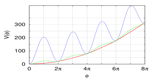
Figure 2: Potential energy $V(\phi)=\beta(1-\cos\phi)+{1\over 2}\phi^{2}$ with three different values of $\beta$, $\beta=1,9.76$ and $100$.

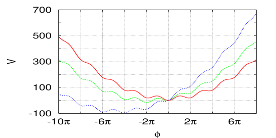
Figure 3: Potential energy $V(\phi)=\beta(1-\cos\phi)+{1\over 2}\phi^{2}+h\phi$ for three different values of the static incident flux $\phi_{e}=0$ in continuous line (red online), $\phi_{e}=1.8\pi$ in dashed line (green online) and $\phi_{e}=4.5\pi$ in short dashed line (blue online).

Fig. 4 shows the phase portrait for $\beta=9.76$. For this value there are only five fixed points. Notice the closed orbits around the fixed points, the closed orbits surrounding the three stable fixed points.

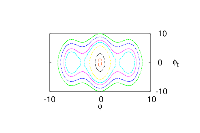
Figure 4: Phase portrait $(\phi,\phi_{t})$ of the Hamiltonian system (15) ($\alpha=0$) for $\beta=9.76$. The contour levels presented are 0.1, 1, 5, 17., 25.0360499136927 (separatrix) , 30.,40. and 50.

We have shown that the steady states of the split-ring Josephson oscillator are similar to the stationary states of atoms. The values $V(\phi)$ near $2n\pi$ are the analog of atomic energy levels. In the quantum regime we should observe Metastability of these states, i.e. there should be quantum tunneling through the barriers at the $n\pi$ positions. This would result in a finite life time of these steady states. In the next section, we will select the incident flux $\phi_{e}$ to move the system from one equilibrium to another.

IV Influence of damping

We consider now that the state of the system can be shifted from one fixed point to another via an incident flux. For a short lived perturbation, the system then relaxes freely to a minimum of energy. The influence of the damping is essential , it should be present to allow the relaxation but small to preserve the picture of the potential. To examine how an incident flux will shift the system from one equilibrium position to another it is useful to analyze the work equation. To obtain it, we multiply (9) by $\phi_{t}$ and integrate over time. We get the difference in energy

$$E(t_{2})-E(t_{1})\equiv[{1\over 2}\phi_{t}^{2}+\beta(1-\cos\phi)+{1\over 2}\phi^{2}]_{t_{1}}^{t_{2}}=\int_{t_{1}}^{t_{2}}dt\phi_{e}\phi_{t}-\alpha\int_{t_{1}}^{t_{2}}dt\phi_{t}^{2}.$$ (20)

The first term on the right hand side is the forcing while the second one is the damping term. When a square pulse is applied to the system, such that

$$\phi_{e}(t)=a,~{}{\rm for}~{}t_{1}<t<t_{2},~{}~{}~{}0~{}~{}{\rm elsewhere}$$

the first integral is $a[\phi(t_{2})-\phi(t_{1})]$. If the system is started at $(0,0)$ in phase space so that the $E(t_{1})=0$ and $\phi(t_{1})=0$, we have

$$E(t_{2})=a\phi(t_{2})-\alpha\int_{t_{1}}^{t_{2}}dt\phi_{t}^{2},$$

so that $\phi(t_{2})$ determines how much energy is fed into the system. When the pulse is long $t_{2}>>t_{1}$ $\phi(t)$ will relax and oscillate so that there are values of $t_{2}$ such that $\phi(t_{2})~{}0$. In that case no energy gets fed into the system. A sure way to avoid this is to take a narrow pulse.

The natural frequency of the oscillator around the $(0,0)$ fixed point is

$$\omega_{0}=\sqrt{\beta+1},$$ (21)

which for $\beta=9.76$ gives $\omega_{0}\approx 3.28$ and a period $T_{0}=2\pi/\omega_{0}\approx 1.91$. To simplify matters we now consider a pulse of duration much smaller than $T_{0}$. This is experimentally feasible and can be modeled using a Dirac delta function $\phi_{e}(t)=a\delta(t)$, where $a$ is a parameter. Let us analyze briefly the solution. The equation (9) becomes

$$\phi_{tt}+(\alpha+\delta)\phi_{t}+\beta\sin(\phi)+\phi=a\delta(t).$$ (22)

Integrating the equation on a small interval of size $\epsilon$ around 0, we get

$$[\phi_{t}]_{-\epsilon}^{\epsilon}+\alpha[\phi]_{-\epsilon}^{\epsilon}+\int_{-\epsilon}^{\epsilon}dt(\beta\sin\phi+\phi)=a.$$ (23)

We now take the limit $\epsilon\to 0$. We will assume continuity of the phase so that $[\phi]_{-\epsilon}^{\epsilon}\to 0$. The third term being the integral of a continuous function tends to 0 when the bounds tend to 0. Assuming $\phi_{t}(0_{-})=0$ we get $\phi_{t}(0_{+})=a$ so that such a short incident pulse will just give momentum to the system.

We will now explore systematically the plane $(\alpha,a)$ characteristic of the incident pulse. The equation (9) has been solved numerically using a Runge-Kutta algorithm with step correction of order 4 and 5.

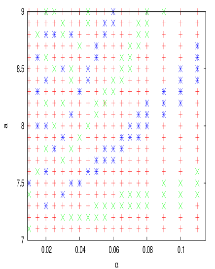
Figure 5: Parameter plane $(\alpha,a)$ showing the different final states reached by the system, the left focus $*$ (blue online), the center focus $+$ (red online) and the right focus $\times$ (green online). The parameter $\beta=9.76$.

The plot in the $(\alpha,a)$ parameter plane shown in Fig. 5 shows the final states, $O$ the central focus ($+$), $R$ the right focus ($\times$) and $L$ the left focus $*$ reached by the system. Notice how these are organized in ”tongues” following the sequence $O~{}R~{}O~{}L~{}O~{}R~{}O~{}L\dots$ as one sweeps the plane counterclock-wise starting from the horizontal axis. This simple geometrical picture can be understood by examining Fig. 4. In the case of small damping, the separatrices around the fixed points are not affected very much. Their perimeter is proportional to the probability of reaching one fixed point or another. The system is moving clock-wise along the orbits. Assume the system reaches the central point $O$ for a given set of parameters. If the damping is increased, the orbit might not reach $O$ but will settle in $L$. Similarly if more kinetic energy is given to the oscillator, it might reach $R$ instead of $O$.

Another important point is that the impulse given to the resonator must be very short so that it relaxes following a free dynamics. The typical frequencies of these devices are about 500 GHz so the impulse must be around 5 Thz which is close to the frequency provided by a laser. This seems to indicate that an optical pulse generated by a laser would be the optimal candidate to switch the device.

To prepare the artificial in a given state, one needs to know if this state is really reached. For that one can use the pump-probe approach: a first pulse is sent to shift the system in the right state, then a small second pulse is sent to analyze the state by reflection or transmission. This is the object of the next section.

V Microwave spectroscopy of the split-ring resonator

We consider here that the split-ring Josephson resonator is subject to irradiation by a microwave field and compute using a scattering theory formalism the response of the system. This field could be microwave radiation from a wave-guide or it could be a laser beam shining on the device. The equations describing the system light-ring are the the generalized pendulum equation for the flux (6) and the the Maxwell equation for the electromagnetic field

$$\nabla\times{\bf E}=-{\bf H}_{t}-{\bf M}_{t},~{}~{}\nabla\times{\bf H}={\bf E}_{t},$$ (24)

where ${\bf E}$ is the electric field, ${\bf H}$ the magnetic field and ${\bf M}$ the magnetization. Taking the curl of the second equation we get the vector wave equation

$$\nabla\times(\nabla\times{\bf H})={\bf H}_{tt}+{\bf M}_{tt}.$$ (25)

If we assume that the wave propagates along $z$ and is transversely polarized so that ${\bf H}$ is parallel to $x$, the normal to the plane of the split ring, and ${\bf E}$ is parallel to $y$. Then we get the scalar wave equation for $H$

$$\Delta H-H_{tt}=M_{tt}.$$ (26)

The magnetization is related to the current $I$ in the loop by

$$M=SI,$$ (27)

where $S$ is the surface enclosed by the ring. Combining (26) with (27) and recalling the expression of the current $I$ given by the term in brackets in (6) we get the final system of equations

$$H_{zz}-{1\over c^{2}}H_{tt}=-{1\over c^{2}}\left({-\Phi_{tt}\over S}+H_{tt}\right)l\delta(z),$$

(28)

$$L(C\Phi_{tt}+{\Phi_{t}\over R}+I_{c}\sin({\Phi\over\phi_{0}}))+\Phi=HS,$$

where $l$ is the film thickness.

We introduce the units of flux, magnetic field, time and space

$$\phi_{0}={\hbar\over 2e},~{}~{}H_{0}={\phi_{0}\over S},~{}~{}\omega_{T}={1\over\sqrt{LC}},~{}~{}l_{0}={c\over\omega_{T}}.$$ (29)

With these units we normalize time, space, the phase and the field as

$$\tau=\omega_{T}t,~{}~{}\zeta={z\over l_{0}},~{}~{}\tilde{\Phi}={\Phi\over\phi_{0}},~{}~{}\tilde{H}={H\over H_{0}}.$$ (30)

The normalized system obtained from (28) is then

$$\tilde{H}_{\zeta\zeta}-\tilde{H}_{\tau\tau}=-\gamma\left(-\tilde{\Phi}_{\tau\tau}+\tilde{H}_{\tau\tau}\right)\delta(\zeta),$$

(31)

$$\tilde{\Phi}_{\tau\tau}+\alpha\tilde{\Phi}_{\tau}+\beta\sin(\tilde{\Phi})+\tilde{\Phi}=\tilde{H},$$

where we have introduced

$$\alpha={\omega_{T}L\over R},~{}~{}\beta={LI_{c}\over\phi_{0}},~{}~{}\gamma={l\over l_{0}}.$$ (32)

We assume that the ring is submitted to a fixed magnetic field $h_{s}$ to which it responds with a constant flux $\phi_{s}$. Then we send in a small electromagnetic pulse $\delta\tilde{H}$ and examine the response $\delta\tilde{\Phi}$ of the ring using the scattering theory. The linearized equations for $\delta\tilde{H},~{}\delta\tilde{\Phi}$ read

$$\delta\tilde{H}_{\zeta\zeta}-\delta\tilde{H}_{\tau\tau}=-\gamma\left(-\delta\tilde{\Phi}_{\tau\tau}+\delta\tilde{H}_{\tau\tau}\right)\delta(\zeta),$$

$$\delta\tilde{\Phi}_{\tau\tau}+\alpha\delta\tilde{\Phi}_{\tau}+\beta\cos(\phi_{s})\delta\tilde{\Phi}+\delta\tilde{\Phi}=\delta\tilde{H}.$$

We now assume periodic solutions

$$\delta\tilde{H}=he^{i\omega\tau},~{}\delta\tilde{\Phi}=\phi e^{i\omega\tau},$$ (34)

and obtain the reduced system

$$h_{\zeta\zeta}+\omega^{2}h=\gamma\omega^{2}\left(-\phi+h\right)\delta(\zeta),$$

(35)

$$\left[-\omega^{2}+i\alpha\omega+1+\beta\cos(\phi_{s})\right]\phi=h.$$

In the scattering we assume the electromagnetic wave to be incident from the left of the film located at $\zeta=0$. We then have

$$h=e^{-i\omega\zeta}+Re^{i\omega\zeta}~{},\zeta<0~{};~{}~{}~{}~{}h=Te^{-i\omega\zeta},\zeta>0~{}~{},$$ (36)

where $R$ is the amplitude of the reflected wave and $T$ the amplitude of the transmitted wave. We have the following interface conditions at $\zeta=0$

$$h(0^{-})=h(0^{+}),~{}~{}[h_{\zeta}]_{0^{-}}^{0^{+}}=\omega^{2}\gamma\left(-\phi(0)+h(0)\right).$$ (37)

They imply the two equations for $R$ and $T$

$$1+R = T,$$

$$-T-(-1+R) = -i\omega\gamma T\left[{-1\over-\omega^{2}+i\alpha\omega+1+\beta\cos(\phi_{s})}+1\right],$$

from which we obtain the transmission coefficient,

$$T={2(-\omega^{2}+1+\beta\cos\phi_{s}+i\omega\alpha)\over D},$$ (38)

the reflection coefficient

$$R={-\alpha\gamma\omega^{2}+i\gamma\omega(\beta\cos\phi_{s}-\omega^{2})\over D},$$ (39)

and where the denominator is

$$D=2(-\omega^{2}+1+\beta\cos\phi_{s})+\alpha\gamma\omega^{2}+i[2\alpha\omega-\gamma\omega(\beta\cos\phi_{s}-\omega^{2})].$$ (40)

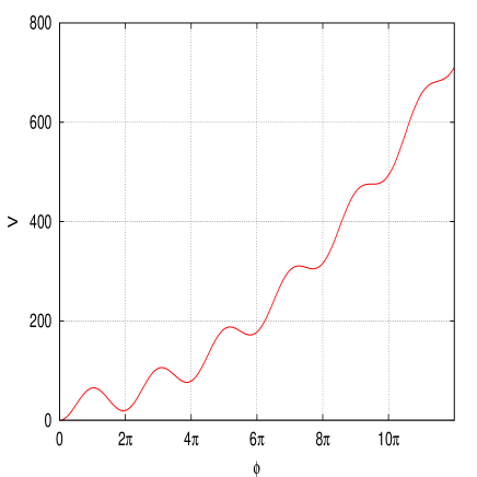
Figure 6: Plot of the potential $V(\phi)$ for $\beta=30$.

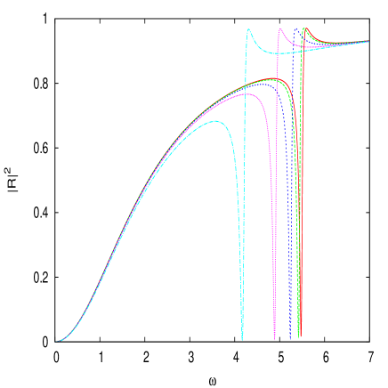
Figure 7: Square of the modulus of the reflection coefficient $|R|^{2}$ as a function of the frequency $\omega$ for the five different equilibria $\phi_{s}=0$ continuous line (red online) and $\phi_{s}=2\pi(1-1/\beta)$ dashed line (green online). The parameters are $\beta=9.76,~{}~{}\gamma=1$ and $\alpha=0.01$.

The square of the modulus of $R$ is

$$|R|^{2}={\alpha^{2}\gamma^{2}\omega^{4}+\gamma^{2}\omega^{2}(\beta\cos\phi_{s}-\omega^{2})^{2}\over|D|^{2}}.$$ (41)

As seen in section 3, the split-ring oscillator has a finite number of equilibria $\phi_{s}$ depending on the parameter $\beta$. As an example we consider $\beta=30$ for which the potential $V(\phi)$ is shown in Fig. 6. The square of the modulus of the reflection coefficient (41) is plotted in Fig. 7 for the five different equilibria. For $\omega\to 0~{}~{}|R|^{2}\to 0$ as $\omega^{2}$ , for $\omega\to\infty$ $|R|^{2}\to 1$. At some $\omega_{s}$ the transmission goes to 0, i.e. the medium becomes transparent. Notice the difference with a real atom which would absorb incident radiation for certain frequencies. The expression for these resonant frequencies $\omega_{s}$ can be obtained by considering the minima of $|R|^{2}$. These correspond to the second term in the numerator of (41) being zero. We get

$$\omega_{s}=\sqrt{\beta\cos\phi_{s}}.$$ (42)

In the example shown, the spectroscopy data $(\omega_{s},\phi_{s})$ is given in table 1.

$\omega_{s}$	5.477	5.420	5.238	4.888	4.169
$\phi_{s}$	0	6.08	12.15	18.2	24.18

Table 1: Spectroscopy data $(\omega_{s},\phi_{s})$ for a split-ring oscillator with five steady states. The parameters are $\beta=30,~{}\gamma=1,~{}\alpha=0.01$.

VI Conclusion

We have derived and analyzed a model for split ring Josephson resonator or RF SQUID in the superconducting regime. If the parameters of the device are chosen appropriately, there exist excited states whose number can be controlled by carefully tuning the inductance and capacity of the ring. We assumed that there are just two excited states and showed how an incident magnetic flux can shift the system from the ground state to one of these excited states. The existence of these excited states makes this system similar to an artificial atom with discrete energy levels. The Josephson oscillator is a unique nonlinear element which allows this. Other nonlinear elements like a diode Lapin:2003 , a Kerr material Zharov:2003 or a laser amplifier Gabitov_Kennedy:2010 would not give these discrete levels. In addition, since the oscillator is operating in the superconducting regime the losses are very small as opposed to the current meta-materials.

By sending a microwave field on the resonator we can perform a spectroscopy of it and characterize in which state it is. Using a scattering theory formalism we compute the reflection and transmission coefficients for the wave. These coefficients differ clearly whether the system is in the ground state or in an excited state enabling to distinguish them.

Acknowledgements
The authors thank Matteo Cirillo and Alexei Ustinov for very helpful discussions. JGC and AM thank the University of Arizona for its support. AIM is grateful to the Laboratoire de Mathématiques, INSA de Rouen for hospitality and support. The computations were done at the Centre de Ressources Informatiques de Haute-Normandie. This research was supported by RFBR grants No. 09-02-00701-a.

References

- (1) Encyclopedia of nonlinear science, A. C. Scott Editor, Routeledge (2001).
- (2) D. R. Tilley, Phys. Lett. 33A, 205, (1970).
- (3) D. Rogovin and M. Scully, Phys. Rep. 25C, 175 (1976).
- (4) P. Barbara, A. B. Cawthorne, S. V. Shitov and C. J. Lobb Phys. Rev. Lett. 82, Nb 9, 1963-1966, (1999).
- (5) I. Ottaviani, M. Cirillo, M. Lucci, V. Merlo, M. Salvato, M. G. Castellano, G. Torrioli, F. Mueller and T. Weimann, Phys. Rev. B 80, 174518, (2009).
- (6) L. Ozyuzer, A. E. Koshelev, C. Kurter, N. Gopalsami, Q. Li, M. Tachiki, K. Kadowaki, T. Yamamoto, H. Minami, H. Yamaguchi, T. Tachiki, K. E. Gray, W.-K. Kwok, and U. Welp, Science 318, 1291, (2007).
- (7) A. Barone and G. Paterno, Physics and Applications of the Josephson effect, J. Wiley, (1982).
- (8) K. Likharev, Dynamics of Josephson junctions and circuits, Gordon and Breach, (1986).
- (9) V. Veselago, L. Braginsky, V. Shklover, Ch. Hafner, Negative Refractive Index Materials J. Computational and Theoretical Nanoscience. 3, 1-30 (2006)
- (10) J.B. Pendry, Negative refraction, Contemporary Physics. 45, 191-202 (2004)
- (11) A.A. Zharov, I.V. Shadrivov, and Yu. S. Kivshar, Nonlinear Properties of Left-Handed Metamaterials, Phys.Rev.Lett. 91, 037401 (2003)
- (12) M. Lapine, M. Gorkunov, and K. H. Ringhofer Nonlinearity of a metamaterial arising from diode insertions into resonant conductive elements, Phys.Rev. B67, No.6, 065601(R), (2003)
- (13) I.R. Gabitov, B. Kennedy, A.I. Maimistov, IEEE Journal of Selected Topics in Quantum Electronics 16, No.2, 401 - 409 (2010)
- (14) N. Lazarides, M. Eleftheriou, and G. P. Tsironis1, Discrete Breathers in Nonlinear Magnetic Metamaterials, Phys.Rev.Lett. 97, 157406 (2006)
- (15) N. Lazarides and G. P. Tsironis, rf superconducting quantum interference device metamaterials, Appl. Phys. Lett. 90, 163501, (2007).
- (16) Andrei I. Maimistov, Ildar Gabitov, Opt.Commun. 283, ¹8, 1633-1639 (2010)
- (17) A.I. Maimistov, I.R. Gabitov, Nonlinear optical effects in artificial materials, Eur. Phys. J. Special Topics. 147,(1), 265-286 (2007)