Excluded-volume effects in the diffusion of hard spheres

Abstract

Excluded-volume effects can play an important role in determining transport properties in diffusion of particles. Here, the diffusion of finite-sized hard-core interacting particles in two or three dimensions is considered systematically using the method of matched asymptotic expansions. The result is a nonlinear diffusion equation for the one-particle distribution function, with excluded-volume effects enhancing the overall collective diffusion rate. An expression for the effective (collective) diffusion coefficient is obtained. Stochastic simulations of the full particle system are shown to compare well with the solution of this equation for two examples.

I Introduction

Recently there has been an increasing interest in understanding the transport of particles with size-exclusion Sun and Weinstein (2007). Size exclusion is important in many biological processes, including diffusion through ion channels Hille (2001); Gillespie et al. (2002) and in chemotaxis Lushnikov et al. (2008), and can have a significant impact on the thermodynamics and kinetics of biological processes such as association reactions at membranes Kim and Yethiraj (2010). Finite-size effects are also important when considering the combustion of powders Saxena (1990), collective behavior (e.g. animal flocks or traffic movement) Camazine et al. (2003); Schadschneider (2002) and granular gases Barrat et al. (2005).

Excluded-volume or steric interactions arise from the mutual impenetrability of finite-size particles (see Fig. 1). For one-dimensional configurations, such as channels, the single-file diffusion of hard-core particles can be solved exactly by mapping it to the classical diffusion of point-particles Lizana and Ambjörnsson (2009); Henle et al. (2008). This has recently been extended to heterogeneous particles and anomalous particles Flomenbom (2010, 2011). However, the situation in higher dimensions is more challenging.

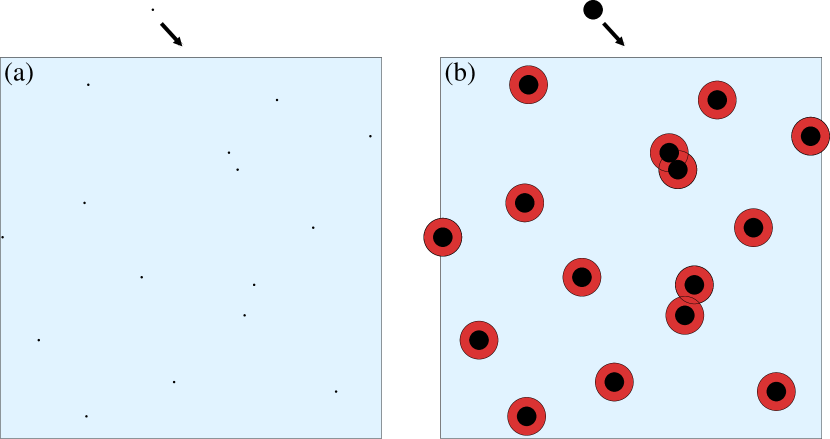
Figure 1: (Color online) Excluded [red (dark grey) and black] and available [blue (light grey)] area in a solution of black particles for the placement of an additional test particle. (a) The area available with point particles is the whole domain. (b) The area available (to the center of the test particle) with finite-size particles is reduced. Modified from Minton Minton (2001).

It is well-known that for finite-size particles the effective diffusion coefficient becomes concentration-dependent. In fact we have to distinguish between two alternative notions of diffusion coefficient: the collective diffusion coefficient, which describes the evolution of the total concentration, and the self-diffusion coefficient, which describes the evolution of a single tagged particle Hanna et al. (1982). Here we concentrate on collective diffusion, hereafter simply referred to as diffusion.

Batchelor Batchelor (1976) models Brownian diffusion of particles with hydrodynamic interaction using generalized Einstein relations to find a concentration dependent correction to the collective diffusion coefficient. Felderhof Felderhof (1978) considers the same problem through an analysis of the Fokker-Planck equation, and includes both excluded volume and hydrodynamic effects. His analysis is based on the thermodynamic limit (in which the number of particles $N$ and the system volume $V$ tend to infinity, with the concentration $N/V$ fixed), and is valid only for a small perturbation from the equilibrium concentration. Similarly, the self-diffusion coefficient to first-order in a constant concentration is obtained from the generalized Smoluchowski equation in Hanna et al. (1982); Ackerson and Fleishman (1982).

Muramatsu and Minton Muramatsu and Minton (1988) use a simple model to calculate the diffusion coefficient of hard spheres by estimating the probability that the target volume for a step in a random walk is free of any macromolecules. Other authors model excluded volume phenomenologically by introducing a particle pressure, resulting in an equation of state in which the compressibility is reduced as the concentration increases Degond et al. (2010).

Another popular approach is to consider lattice models, in which a particle can only move to a site if it is presently unoccupied. Such an approach has been used to model diffusion of multiple species with size exclusion effects Burger et al. (2010); Simpson et al. (2009) or to model the effect of crowding on diffusion-limited reaction Schmit et al. (2009).

The preceding approaches are all either phenomenological in nature, restricted to small perturbations from a uniform concentration, or based on the thermodynamic limit in which the number of particles tends to infinity. Here we consider a finite number of finite-sized particles diffusing in a box of fixed size. We perform an asymptotic analysis of the associated Fokker-Planck equation in the limit that the volume fraction of particles is small. Our analysis is systematic, using the method of matched asymptotic expansions, but is not appropriate for concentrations close to the jamming limit.

II Diffusion with finite-size effects

In order to focus on steric effects, we suppose that there are no electrostatic or hydrodynamic interaction forces between particles. We work in $d$ dimensions, where $d$ is either 2 or 3. Thus our starting point is a system of $N$ identical hard core diffusing and interacting spheres (or disks), each with constant diffusion coefficient $D_{0}$ and diameter $K$, in a bounded domain $\Omega$ in ${\mathbb{R}}^{d}$ of typical diameter $L$. By nondimensionalizing length with $L$ and time with $L^{2}/D_{0}$, the size of the domain and the diffusion coefficient may be normalized to unity, while the diameter of the particles becomes $\epsilon=K/L$. We assume that the particles occupy a small volume fraction, so that $N\epsilon^{d}\ll 1$. We denote the centers of the particles by ${\bf X}_{i}(t)\in\Omega$ at time $t\geq 0$, where $1\leq i\leq N$ . Each center evolves according to the stochastic differential equation (SDE)

$$\mathrm{d}{\bf{X}}_{i}\equiv\sqrt{2}\,\mathrm{d}{\bf B}_{i}+{\bf f}_{i}\,\mathrm{d}t,\qquad 1\leq i\leq N,$$ (1)

where the ${{\bf B}}_{i}$ are $N$ independent $d$-dimensional standard Brownian motions and ${\bf f}_{i}$ is the external force on the $i$ th particle. In general this force may include both inter-particle and external interactions, such as electromagnetic, friction, convection and potential forces, in which case ${\bf f}_{i}$ depends on the positions of all the particles $\vec{X}=({\bf X}_{1},\ldots,{\bf X}_{N})$. While soft-core steric effects can also be built into ${\bf f}_{i}$, hard-core collisions can be more easily expressed as reflective boundary conditions on the “collision surfaces” $r=||{\bf X}_{i}-{\bf X}_{j}||=\epsilon$, with $1\leq i<j\leq N$. Since we are focusing on hard-core particle interactions, we restrict ourselves to other external forces of the form

$$\vec{F}(\vec{X})=[{\bf f}({\bf X}_{1}),\dots,{\bf f}({\bf X}_{N})],$$ (2)

where ${\bf f}:\Omega\to\mathbb{R}^{d}$ acts identically on all $N$ particles. We suppose that the initial positions ${\bf X}_{i}(0)$ are also random, and that they are independent and identically distributed.

Let $P({\vec{x}},t)$ be the joint probability density function of the $N$ particles. Then, by the Itô formula, $P(\vec{x},t)$ evolves according to the linear Fokker-Planck partial differential equation (PDE)

$$\frac{\partial P}{\partial t} =\vec{\nabla}_{\vec{x}}\cdot\big{[}\vec{\nabla}_{\vec{x}}\,P-\vec{F}(\vec{x})\,P\big{]}\quad\textrm{in}\quad\Omega_{\epsilon}^{N},$$ (3a)

where $$\vec{\nabla}_{\vec{x}} \vec{\nabla}_{\vec{x}}\,\cdot N \vec{x}=({\bf x}_{1},\dots,{\bf x}_{N})\in\Omega^{N} \Omega^{N} \Omega_{\epsilon}^{N}=\Omega^{N}\setminus\mathcal{B}_{\epsilon} \mathcal{B}_{\epsilon}=\{\vec{x}\in\Omega^{N}:\exists i\neq j\textrm{ such that }||{\bf x}_{i}-{\bf x}_{j}||\leq\epsilon\} \partial\Omega_{\epsilon}^{N}$$ and respectively stand for the gradient and divergence operators with respect to the -particle position vector . Note that because of steric effects, (3a) is not defined in but in its “hollow form” , where is the set of all illegal configurations (with at least one overlap). On the collision surfaces we have the reflecting boundary condition

$$\big{[}\vec{\nabla}_{\vec{x}}\,P-\vec{F}(\vec{x})\,P\big{]}\cdot{\vec{n}}=0\quad\text{on}\quad\partial\Omega_{\epsilon}^{N},$$ (3b)

where ${\vec{n}}\in\mathcal{S}^{dN-1}$ denotes the unit outward normal. Since the initial positions of the particles are independent and identically distributed, the initial distribution function $P_{0}(\vec{x})$ is invariant to permutations of the particle labels. The form of (3) then means that $P$ itself is invariant to permutations of the particle labels for all time.

Although linear, the PDE model (3) is very high-dimensional, and it is impractical to solve it directly. Since all the particles are identical, we are interested mainly in the marginal distribution function of the first particle, given by $p({\bf x}_{1},t)=\int P(\vec{x},t)\ \mathrm{d}{\bf x}_{2}\dots\mathrm{d}{\bf x}_{N}.$ We aim to reduce the high-dimensional PDE for $P$ to a low-dimensional PDE for $p$ through a systematic asymptotic expansion as $\epsilon\rightarrow 0$.

II.1 Point particles

In the particular case of point-particles ($\epsilon=0$) the model reduction is straightforward. In this case the $N$ particles are independent and the domain is $\Omega_{\epsilon}^{N}\equiv\Omega^{N}$ (no holes), which implies that the internal boundary conditions in (3b) vanish. Therefore $P(\vec{x},t)=\prod_{i=1}^{N}p({\bf x}_{i},t)$, and

$$\frac{\partial p}{\partial t}({\bf x}_{1},t) ={\boldsymbol{\nabla}}_{{\bf x}_{1}}\cdot\left[{\boldsymbol{\nabla}}_{{\bf x}_{1}}\,p-{\bf f}({\bf x}_{1})\,p\right]\quad\textrm{in}\quad\Omega,$$ (4a)

$$0 =\left[{\boldsymbol{\nabla}}_{{\bf x}_{1}}\,p-{\bf f}({\bf x}_{1})\,p\right]\cdot\boldsymbol{\hat{\bf n}}_{1}\quad\textrm{on}\quad\partial\Omega,$$ (4b)

where $\boldsymbol{\hat{\bf n}}_{1}$ is the outward unit normal to $\partial\Omega$. Note that since the particles are indistinguishable each satisfies the same diffusion equation and boundary condition, so that $P$ is a product of $N$ identical 1-particle distribution functions $p$. If the particles were not identically distributed initially then we would need a different distribution function for each one; although these would all satisfy the same diffusion equation they would have different initial conditions. This point will be important when we go on to consider finite-sized particles.

II.2 Finite-size particles

When $\epsilon>0$, the internal boundary conditions in (3b) mean the particles are no longer independent. When we integrate (3a) over ${\bf x}_{2}$, $\ldots$, ${\bf x}_{N}$ and apply the divergence theorem we end up with surface integrals over the collision surfaces, on which $P$ must be evaluated. However, when the particle volume fraction is small, the volume in $\Omega_{\epsilon}^{N}$ occupied by configurations in which three or more particles are close is small [$O(\epsilon^{2d}N^{2})$] compared to those in which two particles alone are in proximity [$O(\epsilon^{d}N)$]. Thus the dominant contribution to these “collision integrals” corresponds to two-particle collisions. We illustrate our approach for $N=2$; since two-particle collisions dominate the extension to arbitrary $N$ is straightforward. A similar approach is used in Hanna et al. (1982); Ackerson and Fleishman (1982).

For two particles at positions ${\bf x}_{1}$ and ${\bf x}_{2}$, Eq. (3a) reads

$$\frac{\partial P}{\partial t}({\bf x}_{1},{\bf x}_{2},t)= \phantom{+}{\boldsymbol{\nabla}}_{{\bf x}_{1}}\cdot\left[{\boldsymbol{\nabla}}_{{\bf x}_{1}}P-{\bf f}({\bf x}_{1})P\right]$$

$$+{\boldsymbol{\nabla}}_{{\bf x}_{2}}\cdot\left[{\boldsymbol{\nabla}}_{{\bf x}_{2}}P-{\bf f}({\bf x}_{2})P\right],$$ (5a)

for $$({\bf x}_{1},{\bf x}_{2})\in\Omega_{\epsilon}^{2}$$, and the boundary condition (3b) reads

$$\left[{\boldsymbol{\nabla}}_{{\bf x}_{1}}P-{\bf f}({\bf x}_{1})P\right]\cdot\boldsymbol{\hat{\bf n}}_{1}+\left[{\boldsymbol{\nabla}}_{{\bf x}_{2}}P-{\bf f}({\bf x}_{2})P\right]\cdot\boldsymbol{\hat{\bf n}}_{2}=0,$$ (5b)

on ${\bf x}_{i}\in\partial\Omega$ and $||{\bf x}_{1}-{\bf x}_{2}||=\epsilon$. Here $\boldsymbol{\hat{\bf n}}_{i}={{\bf n}}_{i}/||{{\bf n}}_{i}||$, where ${{\bf n}}_{i}$ is the component of the normal vector $\vec{n}$ corresponding to the $i-$th particle, $\vec{n}=({\bf n}_{1},{\bf n}_{2})$. We note that $\boldsymbol{\hat{\bf n}}_{1}=0$ on ${\bf x}_{2}\in\partial\Omega$, and that $\boldsymbol{\hat{\bf n}}_{1}=-\boldsymbol{\hat{\bf n}}_{2}$ on $||{\bf x}_{1}-{\bf x}_{2}||=\epsilon$.

We denote by $\Omega({\bf x}_{1})$ the region available to particle 2 when particle 1 is at ${\bf x}_{1}$, namely $\Omega({\bf x}_{1})=\Omega\setminus B_{\epsilon}({\bf x}_{1})$. Note that when the distance between ${\bf x}_{1}$ and $\partial\Omega$ is less than $\epsilon$ the volume $|\Omega({\bf x}_{1})|$ increases. This creates a boundary layer of width $\epsilon$ around $\partial\Omega$ where there exists a wall-particle-particle interaction (three-body interaction). Since the dimensions of the container are much larger than the particle diameter these interactions are higher-order and we may safely ignore them and take $|\Omega({\bf x}_{1})|$ constant . Integrating Eq. (5a) over $\Omega({\bf x}_{1})$ yields

$$\frac{\partial p}{\partial t}({\bf x}_{1},t)=\phantom{-}{\boldsymbol{\nabla}}_{{\bf x}_{1}}\cdot\left[{\boldsymbol{\nabla}}_{{\bf x}_{1}}\,p-{\bf f}({\bf x}_{1})\,p\right]$$

$$\mbox{}+\int_{\partial B_{\epsilon}({\bf x}_{1})}[{\bf f}({\bf x}_{1})\,P-2{\boldsymbol{\nabla}}_{{\bf x}_{1}}P-{\boldsymbol{\nabla}}_{{\bf x}_{2}}P]\cdot{\boldsymbol{\hat{\bf n}}}_{2}\,\mathrm{d}S_{2}\qquad$$

$$\mbox{ }+\int_{\partial\Omega\cup\partial B_{\epsilon}({\bf x}_{1})}\left[{\boldsymbol{\nabla}}_{{\bf x}_{2}}\,P-{\bf f}({\bf x}_{2})\,P\right]\cdot{\boldsymbol{\hat{\bf n}}}_{2}\,\mathrm{d}S_{2}.$$

The first integral in (II.2) comes from switching the order of integration with respect to ${\bf x}_{2}$ and differentiation with respect to ${\bf x}_{1}$ using the transport theorem; the second comes from using the divergence theorem on the derivatives in ${\bf x}_{2}$. Using (5b) and rearranging we find

$$\frac{\partial p}{\partial t}({\bf x}_{1},t)=\phantom{-}{\boldsymbol{\nabla}}_{{\bf x}_{1}}\cdot\left[{\boldsymbol{\nabla}}_{{\bf x}_{1}}\,p-{\bf f}({\bf x}_{1})\,p\right]$$ (7)

$$\mbox{ }+\int_{\partial B_{\epsilon}({\bf x}_{1})}\left\{-2{\boldsymbol{\nabla}}_{{\bf x}_{1}}P+P\left[{\bf f}({\bf x}_{1})-{\bf f}({\bf x}_{2})\right]\right\}\cdot{\boldsymbol{\hat{\bf n}}}_{2}\,\mathrm{d}S_{2}.\qquad$$

Because the pairwise particle interaction is localized near the collision surface $\partial B_{\epsilon}({\bf x}_{1})$ we can determine it using the method of matched asymptotic expansions Holmes (1995).

II.3 Matched asymptotic expansions of the density $P$

We suppose that when two particles are far apart ($||{\bf x}_{1}\!-{\bf x}_{2}||\gg\epsilon$) they are independent, whereas when they are close to each other ($||{\bf x}_{1}-{\bf x}_{2}||\sim\epsilon$) they are correlated. We designate these two regions of the configuration space $\Omega_{\epsilon}^{2}$ the outer region and inner region, respectively.

In the inner region, we set ${\bf x}_{1}=\tilde{\bf x}_{1}$ and ${\bf x}_{2}=\tilde{\bf x}_{1}+\epsilon\tilde{\bf x}$ and define $\tilde{P}(\tilde{\bf x}_{1},\tilde{\bf x},t)=P({\bf x}_{1},{\bf x}_{2},t)$. With this rescaling (5) becomes

$$\epsilon^{2}\frac{\partial\tilde{P}}{\partial t}(\tilde{{\bf x}}_{1},\tilde{\bf x},t)=2{\boldsymbol{\nabla}}_{\tilde{{\bf x}}}^{2}\,\tilde{P}-\epsilon^{2}{\boldsymbol{\nabla}}_{\tilde{\bf x}_{1}}\cdot\big{[}{\bf f}(\tilde{\bf x}_{1})\tilde{P}\big{]}+\epsilon^{2}{\boldsymbol{\nabla}}_{\tilde{\bf x}_{1}}^{2}\,\tilde{P}$$ (8a)

$$\mbox{}+\epsilon{\boldsymbol{\nabla}}_{\tilde{\bf x}}\cdot\big{\{}\left[{\bf f}(\tilde{\bf x}_{1})-{\bf f}(\tilde{\bf x}_{1}+\epsilon\tilde{\bf x})\right]\tilde{P}\big{\}}-2\epsilon{\boldsymbol{\nabla}}_{\tilde{{\bf x}}_{1}}\!\cdot\!{\boldsymbol{\nabla}}_{\tilde{\bf x}}\tilde{P},\qquad$$

with

$$2\tilde{\bf x}\cdot{\boldsymbol{\nabla}}_{\tilde{\bf x}}\tilde{P} = \epsilon\,\tilde{\bf x}\cdot\big{\{}{\boldsymbol{\nabla}}_{\tilde{\bf x}_{1}}\tilde{P}+\left[{\bf f}(\tilde{\bf x}_{1}+\epsilon\tilde{\bf x})-{\bf f}(\tilde{\bf x}_{1})\right]\tilde{P}\big{\}},\qquad$$ (8b)

on $$||\tilde{\bf x}||=1 \tilde{\bf x}_{1} \partial\Omega \tilde{\bf x}\rightarrow\infty$$. As noted above, we can neglect the boundary layer and hence assume that is not close to ; the region in which the particles are close to each other and the boundary is even smaller, and will affect only the higher-order terms. In addition to (8b) the inner solution must match with the outer solution as . In the outer region, by independence,

$$P({\bf x}_{1},{\bf x}_{2},t)=q({\bf x}_{1},t)q({\bf x}_{2},t),$$

for some function $$q({\bf x},t) P q P q({\bf x}_{1},t)=p({\bf x}_{1},t)+\mathcal{O}(\epsilon^{d})$$. Note that the invariance of with respect to a switch of particle labels means that in the outer region both particles have the same distribution function (as happened in the point particle case). The normalization condition on gives . Expanding this outer solution in inner variables gives

$$P({{\bf x}}_{1},{\bf x}_{2},t) = q(\tilde{{\bf x}}_{1},t)q(\tilde{\bf x}_{1}+\epsilon\tilde{{\bf x}})$$ (8c)

$$\sim q^{2}(\tilde{\bf x}_{1},t)+\epsilon q(\tilde{{\bf x}}_{1})\,\tilde{\bf x}\cdot{\boldsymbol{\nabla}}_{\tilde{\bf x}_{1}}q(\tilde{\bf x}_{1})+\cdots.\qquad$$

Expanding $\tilde{P}$ in powers of $\epsilon$, and solving (8a), (8b) with the matching condition (8c) we find that the solution in the inner region is simply

$$\tilde{P}(\tilde{\bf x}_{1},\tilde{\bf x},t)\sim q^{2}(\tilde{\bf x}_{1},t)+\epsilon q(\tilde{{\bf x}}_{1})\,\tilde{\bf x}\cdot{\boldsymbol{\nabla}}_{\tilde{\bf x}_{1}}q(\tilde{\bf x}_{1})+\cdots.$$ (9)

Using this solution to evaluate the integrals in (7) we find, to $O(\epsilon^{d})$,

$$\frac{\partial p}{\partial t}({\bf x}_{1},t)=\ {\boldsymbol{\nabla}}_{{\bf x}_{1}}\cdot\left[{\boldsymbol{\nabla}}_{{\bf x}_{1}}\!\left(p+\alpha_{d}\epsilon^{d}p^{2}\right)-{\bf f}({\bf x}_{1})\,p\right],$$ (10)

where $\alpha_{2}=\pi/2$ and $\alpha_{3}=2\pi/3$. The extension from two particles to $N$ particles is straightforward up to $O(\epsilon^{d})$, since at this order only pairwise interactions need to be considered. Particle 1 has $(N-1)$ inner regions, one with each of the remaining particles. A similar procedure shows that the marginal distribution function satisfies

$$\frac{\partial p}{\partial t}({\bf x}_{1},t) ={\boldsymbol{\nabla}}_{{\bf x}_{1}}\!\cdot\!\big{\{}{\boldsymbol{\nabla}}_{{\bf x}_{1}}\!\left[p+\alpha_{d}(N\!-\!1)\epsilon^{d}p^{2}\right]-{\bf f}({\bf x}_{1})\,p\big{\}}.$$ (11)

Equation (11) describes the probability distribution function for finding the first particle at position $x_{1}$ at time $t$. Since the system is invariant to permutations of the particle labels, the marginal distribution function of any other particle is the same. Thus the probability distribution function for finding any particle at position $x_{1}$ at time $t$ is simply $Np$.

II.4 Interpretation

We see from (11) that steric interactions lead to a concentration-dependent diffusion coefficient, with the additional term proportional to the excluded volume. Equation (11) is consistent with that derived by Felderhof Felderhof (1978), but extends it to situations in which $p$ is not close to uniform. We emphasize that (11) is valid for any $N$. However, for large $N$ such that $N-1\approx N$ we can introduce the volume concentration $c=\pi N\epsilon^{d}p/2d$ and rewrite (11) as

$$\frac{\partial c}{\partial t}({\bf x}_{1},t)={\boldsymbol{\nabla}}_{{\bf x}_{1}}\!\cdot\!\big{\{}D(c)\,{\boldsymbol{\nabla}}_{{\bf x}_{1}}\!c-{\bf f}({\bf x}_{1})\,c\big{\}},$$ (12)

where $D(c)$ is the concentration-dependent collective diffusion coefficient, given by

$$D(c)=1+4(d-1)c.$$ (13)

Note that the collective diffusion coefficient $D(c)$ is increased relative to point particles. This is in contrast to the self-diffusion coefficient (which may be related to the mean squared displacement of a particular particle) which is reduced relative to point particles Hanna et al. (1982). This apparent contradiction may be understood as follows: the diffusion of any particular particle is impeded by its collisions with other particles. However, these collisions bias the random walk towards areas of low particle density, so that the overall spread of all particles is faster. To analyze the self-diffusion coefficient in the current framework we would need to label a particular particle, rather than treating all particles as identical.

Whilst the self-diffusion coefficient can be thought of a diffusion coefficient intrinsically attached to each particle, the collective diffusion coefficient relates the diffusive flux to the concentration gradient of all particles Mazo (2002): the distribution function $p$ is the probability of finding any particle at a given position, rather than the probability of finding a particular particle there. Thus the collective diffusion coefficient is not associated with an individual (tagged) particle or even a representative particle. This also means that it cannot easily be related to the mean-squared displacement of particles. This distinction has important consequences when upscaling from individual to collective behavior.

In (11) we have only included the leading-order nonlinear term due to steric effects. There will be correction terms of $O(\epsilon^{d+1}N)$ due to higher-order terms in the two-particle inner solution (9), as well as new inner regions where three particles [$O(\epsilon^{2d}N^{2})$], or two particles and the boundary [$O(\epsilon^{d+1}N)$], are close. The most important of these corrections is that due to interactions between three (or more) particles. Because our asymptotic expansion is systematic, these correction terms could in principle be calculated.

III Comparison with the full particle system

In order to assess the validity of (11) we compare its solution $p({\bf x}_{1},t)$ (obtained by a simple finite difference method) with Monte Carlo (MC) simulations of the $2N$-coupled SDE (1) in two dimensions. The particle-particle (and particle-wall) overlaps are treated as in Strating (1999). To test the importance of steric interactions, we also compare with the corresponding solutions with $\epsilon=0$.

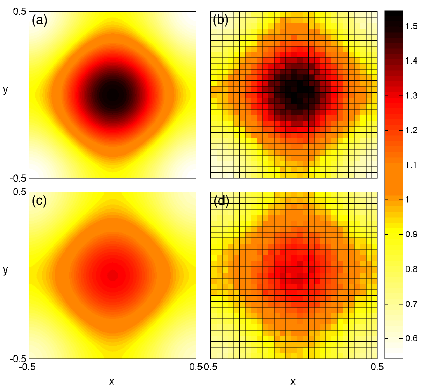
Figure 2: (Color online) Marginal distribution function $p({\bf x}_{1},t)$ at time $t=0.05$ with normally distributed initial data and $N=400$. (a) Solution $p({\bf x}_{1},t)$ of (4) for point particles ($\epsilon=0$). (b) Histogram for $\epsilon=0$. (c) Solution $p({\bf x}_{1},t)$ of (11) for finite-sized particles ($\epsilon=0.01$). (d) Histogram for $\epsilon=0.01$. Histograms computed from $10^{4}$ realizations of (1) with $\Delta t=10^{-5}$. All four plots have the same color bar.

In Fig. 2 we show the results of a time-dependent simulation with ${\bf f}\equiv 0$, $\Omega=[-\tfrac{1}{2},\tfrac{1}{2}]^{2}$, $\epsilon=0.01$, $N=400$, for which the initial distribution is a Gaussian of zero mean and standard deviation 0.09 (normalized so that its integral over $\Omega$ is one); the figures correspond to time $t=0.05$. The simulation time-step $\Delta t$ is chosen such that almost no collisions are missed. The theoretical predictions for both point and finite-size particles compare very well with their simulation counterparts, while steric effects are clearly appreciable even though the volume fraction of particles is only $0.0314$. However, note that while the average concentration is low, the local concentration is considerably high at the origin: $c=0.617$ at time $t=0$ and $c=0.0479$ at time $t=0.05$. The initial profile, in which particles are concentrated in the center, spreads faster when steric effects are included [Fig. 2(c)] than when they are not [Fig. 2(a)], indicating that the overall collective diffusion is enhanced.

When the force field ${\bf f}$ is the gradient of a potential, ${\bf f}({\bf x}_{1})=-{\boldsymbol{\nabla}}_{{\bf x}_{1}}V({\bf x}_{1})$, we may write (11) as

$$\frac{\partial p}{\partial t}={\boldsymbol{\nabla}}_{{\bf x}_{1}}\cdot(p{\bf u}),$$ (14)

with ${\bf u}={\boldsymbol{\nabla}}_{{\bf x}_{1}}\left[\ln p+2\alpha_{d}(N-1)\epsilon^{d}p+V({\bf x}_{1})\right]$. Equation (14) has an associated free energy Carrillo et al. (2003)

$$F(p)=\!\int_{\Omega}p\ln p+\alpha_{d}(N\!-\!1)\epsilon^{d}p^{2}\,\mathrm{d}{\bf x}_{1}+\int_{\Omega}\!V({\bf x}_{1})\,p\,\mathrm{d}{\bf x}_{1},$$

where the first integral corresponds to the internal energy and the second integral is the potential energy. Note that excluded-volume effects increase the internal energy of the system. The stationary distribution, which we denote $p_{s}({\bf x}_{1})$, is obtained by minimizing the free energy or by solving

$$\ln p_{s}({\bf x}_{1})+2\alpha_{d}(N-1)\epsilon^{d}p_{s}({\bf x}_{1})+V({\bf x}_{1})=C,$$ (15)

with the constant $C$ determined by the normalization condition on $p_{s}$. For our second example we consider the volcano-shaped potential $V({\bf x}_{1})=-4.77\,e^{-100||{\bf x}_{1}||^{2}}+3.58\,e^{-50||{\bf x}_{1}||^{2}}$ and we compare the stationary distribution $p_{s}$ predicted by (15) with simulations using the Metropolis-Hastings (MH) algorithm Chib and Greenberg (1995). Figure 3 shows the model and simulation results with $N=1000$ and $\Omega$ and $\epsilon$ as in Fig. 2 for both point and finite-size particles (with volume fraction 0.079 and volume concentration $c=0.189$ at the origin). In this case there is competition between the potential well and steric repulsion: the particle density inside the well is reduced for finite-size particles. Again, the agreement between the model (15) and the stochastic simulations is excellent.

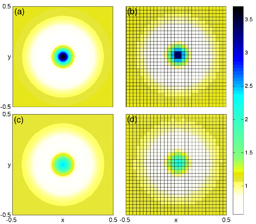
Figure 3: (Color online) Stationary marginal distribution function $p_{s}({\bf x}_{1})$ under the external potential $V$ for point particles and finite-size particles, with $N=1000$. (a) Point particles, $p_{s}\propto e^{-V}$. (b) Histogram for $\epsilon=0$. (c) Finite-size particles $p_{s}$ from (15) ($\epsilon=0.01$). (d) Histogram for $\epsilon=0.01$. Histograms computed with $10^{9}$ steps of the MH algorithm. All four plots have the same color bar.

IV Discussion

We have derived systematically a nonlinear diffusion equation which describes steric interactions in the limit of small but finite particle volume fraction. Our method justifies for example the ansatz made in Calvez and Carrillo (2006) to account for the finite size of the cells in the Keller-Segel model and prevent aggregation, and unlike Felderhof (1978); Beenakker and Mazur (1983) does not rely on a closure assumption.

The equation we have derived is for the one-particle distribution function, which measures the probability of finding any particle at a given position; the particles we consider are identical and indistinguishable. This means that we are examining collective diffusion, and we find that this is enhanced by the finite size of the particles. We have not considered the self-diffusion of a particular (tagged) particle, which can be related to an individual particle’s mean-square displacement. To analyze the self-diffusion coefficient in the current framework we would need to label a particular particle, rather than treating all particles as identical; we intend to do this in a future work in which we consider multiple particle populations.

We note that for point particles in one dimension (where particles must move in single file and are not allowed to pass) Flomenbom and Taloni (2008) has observed density dependence in the self-diffusion (mean square displacement) of a tagged particle. Their interpretation is that the expansion of the whole system from dense to dilute environments quickens the self-diffusion of any tagged particle. This is a different effect to the one we have observed, since, as mentioned in the introduction, the collective diffusion of point particles in one dimension is linear, with a diffusion coefficient independent of the density. In two dimensions self-diffusion is less sensitive to the particle density, since, informally, there is much more space for particles to pass each other.

The method we have developed was implemented here in its simplest setting (hard-core identical spherical particles with an external potential) but it can be extended in many directions. Particles of different size (cf. Bruna and Chapman ) or shape can easily be incorporated, while the hard-core interaction between particles can be replaced by any short-range soft-core interaction.

On the other hand, incorporating long range effects such as chemotaxis or electrostatic interactions is more challenging; in such cases a system size expansion is likely to be needed in addition to a small particle expansion.