Dynamics and interactions of active rotors

Abstract

We consider a simple model of an internally driven self-rotating object; a rotor, confined to two dimensions by a thin film of low Reynolds number fluid. We undertake a detailed study of the hydrodynamic interactions between a pair of rotors and find that their effect on the resulting dynamics is a combination of fast and slow motions. We analyse the slow dynamics using an averaging procedure to take account of the fast degrees of freedom. Analytical results are compared with numerical simulations. Hydrodynamic interactions mean that while isolated rotors do not translate, bringing together a pair of rotors leads to motion of their centres. Two rotors spinning in the same sense rotate with an approximately constant angular velocity around each other, while two rotors of opposite sense, both translate with the same constant velocity, which depends on the separation of the pair. As a result a pair of counter-rotating rotors are a promising model for controlled self-propulsion in two dimensions.

Soft active systems are composed of interacting units that consume energy and generate local motion and mechanical stresses. They show a rich variety of collective behaviour, including dynamical order-disorder transitions and pattern formation on various scales. A much studied example are collections of self-propelled objects  [2, 3, 4, 6, 5, 7, 8, 9, 10, 11, 12, 13, 14, 15, 16] which independently translate due to internally generated motions by the objects themselves.

In this article we study, a particularly simple class of self-driven particles and their interactions. These are self-rotating objects (that we call rotors) lying in a plane [17, 18, 19]. Our motivation is two-fold. First recent developments [20, 21, 22, 23] have shown the possibility of experimentally realising such self-driven rotors on the nano-scale. In addition recent progress in nano-scale microfabrication techniques have been able to generate synthetic chemically driven rotors that rotate fast enough so that the effects of their interactions on their dynamics can been measured experimentally [24]. Second, a collection of active rotors provide a particularly simple example of an active system as their collective behaviour can be described in terms of scalar rather than vector equations. The first step in the quest to understand their collective behaviour is to develop a detailed understanding of their interactions.

Motivated by this we investigate analytically and numerically the dynamics of rotors confined in two dimensions (the $x-y$ plane) by a viscous film, such as a membrane. We first introduce the model of a single rotor: (which when isolated rotates around its centre but does not translate). Each rotor can be described by a scalar $\sigma$, the value of the projection of its angular velocity $\bm{\omega}$ on the $\hat{\bm{z}}$ direction, that we call spin. We next study the hydrodynamic interactions between a pair, in the absence of noise when the distance between their centres is large compared to their size. We find that the resulting dynamics can be described in terms of slow and fast variables that depend on the relative spin of the pair. We obtain analytic expressions for the dynamics of the slowly varying quantities and find that for opposite spins the hydrodynamic interactions lead to a net translation of the pair while for like spins they lead to a relative rotation of the pair around each other. These leading order analytic results are in good agreement with numerical simulations for well separated rotors. Interestingly, our study suggests that a pair of counter-rotating rotors could be used to construct a micron sized-swimmer in two dimensions, with the speed of the swimmer controlled in a precise manner by varying the equal and opposite torques acting on the rotors.

1 Hydrodynamics of a thin fluid film

The active rotors can be confined to two dimensions by being adsorbed onto a thin fluid film  [25, 26, 27, 28, 17, 29]. The film can be described as an infinite incompressible two dimensional layer of fluid with (2d) viscosity $\eta$ filling the plane $z=0$ and coupled hydrodynamically to another incompressible bulk fluid of (3d) viscosity $\eta_{e}$ which fills the region $z\neq 0$ (see Fig. 1). We consider the fluid dynamics in the vanishing Reynolds number (Stokes) limit where inertia can be neglected [30]. Given a force density ${\bm{F}}(x,y)$, the in plane equation reads

$$\eta\nabla_{\perp}^{2}\bm{v}+\nabla_{\perp}p+\sigma^{+}_{e}-\sigma^{-}_{e}=-\bm{F}\;;\;\nabla_{\perp}\cdot\bm{v}=0$$ (1)

where $\bm{v}(x,y)$ is the 2-dimensional velocity field (in the plane $z=0$), $\nabla_{\perp}=(\partial_{x},\partial_{y})$ is the 2-d gradient operator, $p(x,y)$ is the in-plane pressure. $\sigma^{\pm}_{e}:=\eta_{e}\partial_{z}\bm{v}^{\prime}|_{0^{\pm}}$ is the shear stress of the bulk fluid at the top/bottom of the thin film; $\bm{v}^{\prime}(x,y,z)$ is the 3-dimensional velocity field defined in the external region $z\neq 0$ which satisfies the Stokes equation

$$\eta_{e}\nabla^{2}\bm{v}^{\prime}+\nabla p^{\prime}=0\quad;\quad\nabla\cdot\bm{v}^{\prime}=0$$ (2)

where $\nabla=(\nabla_{\perp},\partial_{z})$ is a 3-dimensional gradient operator and $p^{\prime}(x,y,z)$ is the bulk pressure. The ratio of the two and three dimensional viscosities introduces a length-scale $l:=\eta/2\eta_{e}$. Associated with the existence of this length-scale are two asymptotic regimes: at lengths $r\gg l$ dissipation is mostly due to flow out of plane, and the hydrodynamics is similar (but not identical) to that in three dimensions; while for $r\ll l$ dissipation occurs almost entirely in plane and thus hydrodynamic flow fields are quasi-two dimensional. We construct objects out of collections of flat disks of radius $a$ subject to point forces $\mathbf{f}$ at their centres lying entirely in-plane. The viscous drag on a disk moving at a constant speed can be obtained in an analogous way to the Stokes’ solution for a sphere in three dimensions and the resulting drag has the form  [25, 26, 28] $\gamma=4\pi\eta/g$ where $g$ is a function of $l/a$.

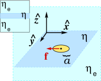
Figure 1: Thin film. A two dimensional fluid layer characterized by a 2d viscosity $\eta$ fills the whole plane $z=0$. It is surrounded, above and below, by another fluid having a 3d viscosity $\eta_{e}$ with which it is coupled hydrodynamically. Objects are constructed out of groups of disks of radius $a$ that are subject to forces lying entirely in the plane $z=0$.

The interaction between disks embedded in the film can be obtained using the Green function $\bm{H}$ of eq. (1), corresponding to the flow, $\bm{v}(\mathbf{r})=\bm{H}(\mathbf{r}-\mathbf{r}_{0})\cdot{\bf f}_{0}$ generated by an in-plane point-like force, or stokeslet, ${\bf f}_{0}$ at ${\bf r}_{0}$. This description is well suited in the limit where the separation between disks is much greater than their radii so they can be approximated as point-like objects. The tensor $\bm{H}({\bf r})={l\over\eta}\int{d^{2}k\over(2\pi)^{2}}e^{-i{\bf k\cdot r}}{\left({\mathbb{I}}-\hat{\bm{k}}\otimes\hat{\bm{k}}\right)\over k^{2}+kl}$ is the thin film equivalent of the Oseen tensor  [31, 29] and we refer to it as the hydrodynamic tensor. In the limit $r\gg l$,

$$\bm{H}(\mathbf{r})=\dfrac{l}{2\pi\eta}\dfrac{\hat{\bm{r}}\otimes\hat{\bm{r}}}{r}+O\left(({l/r})^{2}\right).$$ (3)

For a set of $N$ discs with forces ${\bf f}_{k}$ at their centres, ${\bf r}_{k}$ ($k\in\{1,N\}$) each disk is subject to the dynamic equation

$$\mathbf{v}_{n}=\sum^{N}_{m,n=1}\bm{\mathcal{H}}_{nm}\cdot\mathbf{f}_{m}$$ (4)

where, for $n\neq m$ $\bm{\mathcal{H}}_{nm}:=\bm{H}(\mathbf{r}_{n}-\mathbf{r}_{m})$, and for $n=m$ we have $\bm{\mathcal{H}}_{nn}:=\mathbb{I}/\gamma$. This allows us to characterise the flow fields on scales much larger than $a$.

2 The rotor model

A rotor is composed of two disks, labelled with the index $n=1,2$. The disks are a fixed distance $L$ apart, oriented along the direction $\hat{\bm{u}}$ (lying in-plane). Denoting by $\mathbf{x}_{n}$ the position of the disk $n$, $L\hat{\bm{u}}=\mathbf{x}_{1}-\mathbf{x}_{2}$. Equal and opposite point forces (also lying in-plane) act at the centre of the disks directed perpendicular to their separation, applying a torque on the rotor. The associated force density is $\mathbf{f}_{n}\delta(\mathbf{x}-\mathbf{x}_{n})$, where $\mathbf{f}_{n}:=(-)^{n+1}\sigma f\hat{\bm{u}}^{\perp}$ so that $\mathbf{f}:=\mathbf{f}_{1}=-\mathbf{f}_{2}$. The magnitude of the rotor torque, $fL$ and the spin $\sigma=\pm 1$ (the sense of rotation), parametrise the rotor. The director $\hat{\bm{u}}^{\perp}$ is obtained from $\hat{\bm{u}}$ by a clockwise rotation of an angle $\pi/2$. See Fig. 2 for an illustration. Neglecting thermal noise, the equations of motion are $\dot{\mathbf{x}}_{1}=\left({\mathbb{I}}/\gamma-\bm{\mathcal{H}}_{12}\right)\cdot\mathbf{f}\;,\;\dot{\mathbf{x}}_{2}=-\left({\mathbb{I}}/\gamma-\bm{\mathcal{H}}_{21}\right)\cdot\mathbf{f}\;,$ where $\bm{\mathcal{H}}_{12}=\bm{\mathcal{H}}_{21}=\frac{l}{2\pi\eta}\frac{\hat{\bm{u}}\otimes\hat{\bm{u}}}{L}$.

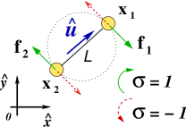
Figure 2: Instantaneous configuration of a single rotor. For fixed $f$, there are 2 possible choices for the force distribution, determined by $\sigma$, as illustrated, resulting in two different senses of rotation. We associate $\sigma=1$ with clockwise rotation and vice-versa for $\sigma=-1$.

By construction, the rotor centre $\mathbf{R}=\frac{1}{2}(\mathbf{x}_{1}+\mathbf{x}_{2})$ is stationary while the orientation axis is not. Its equation $\dot{\hat{\bm{u}}}=\frac{2\mathbf{f}}{L\gamma}$, describes rotation with constant angular velocity around the centre. To see this it is convenient to introduce the normal, $\hat{\bm{z}}$ defined as $\hat{\bm{u}}\wedge\hat{\bm{u}}_{\perp}=\hat{\bm{z}}$, a unit vector in directed along the negative $z-$axis. The equation for $\hat{\bm{u}}$ can then be recast as:

$$\dot{\hat{\bm{u}}}=\bm{\omega}_{0}\wedge\hat{\bm{u}}$$ (5)

with angular velocity, $\bm{\omega}_{0}:=\frac{2f}{L\gamma}\sigma\hat{\bm{z}}$. The period of the rotor is given by $T_{0}:=2\pi/\omega_{0}$, where $\omega_{0}=2f/(L\gamma)$. The spin $\sigma$ is simply the projection of the angular velocity director $\hat{\bm{\omega}}_{0}$ on to $\hat{\bm{z}}$. Equation (5) determines $\hat{\bm{u}}(t)$ up to a phase. We choose $\hat{\bm{u}}=\hat{\bm{x}}\sin(\sigma\omega_{0}t)+\hat{\bm{y}}\cos(\sigma\omega_{0}t)$ and $\hat{\bm{u}}^{\perp}=\hat{\bm{x}}\cos(\sigma\omega_{0}t)-\hat{\bm{y}}\sin(\sigma\omega_{0}t)$.

3 Dynamics of two interacting rotors

It is straightforward to generalize the approach above to deal with two rotors, which we label $A$ and $B$ (see Fig. 3). There are now 4 disks with centres at positions, $\mathbf{x}^{\alpha}_{n}$, where $n=1,2$ and $\alpha=A,B$. It is convenient to describe the dynamics in terms of orientations $\hat{\bm{u}}_{\alpha}$ and the centre positions $\mathbf{R}_{\alpha}$ of each rotor, defined by $L\hat{\bm{u}}_{\alpha}:=\mathbf{x}^{\alpha}_{1}-\mathbf{x}^{\alpha}_{2}\;;\;\mathbf{R}_{\alpha}:=\dfrac{1}{2}(\mathbf{x}^{\alpha}_{1}+\mathbf{x}^{\alpha}_{2})\;,$ respectively. A single rotor cannot propel itself through the fluid. Interestingly, however, net motion of the rotor center occurs when another rotor is close by. This can be seen in the equations of motion for $\mathbf{R}_{\alpha}$ and $\hat{\bm{u}}_{\alpha}$ that, in absence of noise, are :

$$\dot{\hat{\bm{u}}}_{\alpha}=\bm{\omega}^{\alpha}_{0}\wedge\hat{\bm{u}}_{\alpha}+\big{(}\bm{\mathcal{H}}_{1\alpha 1\beta}-\bm{\mathcal{H}}_{1\alpha 2\beta}-\bm{\mathcal{H}}_{2\alpha 1\beta}+\bm{\mathcal{H}}_{2\alpha 2\beta}\big{)}\cdot\dfrac{\mathbf{f}_{\beta}}{L};$$

$$\dot{\mathbf{R}}_{\alpha}=\dfrac{1}{2}\Big{[}\bm{\mathcal{H}}_{1\alpha 1\beta}-\bm{\mathcal{H}}_{1\alpha 2\beta}+\bm{\mathcal{H}}_{2\alpha 1\beta}-\bm{\mathcal{H}}_{2\alpha 2\beta}\Big{]}\cdot\mathbf{f}_{\beta}.$$ (6)

Here $\bm{\mathcal{H}}_{p\alpha q\beta}:=\bm{H}(\mathbf{x}^{\alpha}_{p}-\mathbf{x}^{\beta}_{q})$ is defined for $\alpha\neq\beta$ and $r\gg l,a$. It is convenient to define

$$\mathbf{r} :=\mathbf{R}_{A}-\mathbf{R}_{B};$$

$$\mathbf{R} :=\frac{1}{2}(\mathbf{R}_{A}+\mathbf{R}_{B});$$ (7)

the relative and mean position respectively of the two centres of rotors A and B. The magnitude $r$ of the relative distance $\mathbf{r}$ is the typical separation between the objects. For large separations, $r\gg L$, it is natural to expand the hydrodynamic tensor using the small parameter $\epsilon:=L/r$.

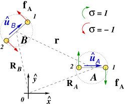
Figure 3: Instantaneous configurations of two interacting rotors. The two rotors, labelled with the letters $A,B$, lie in the plane at a distance $r$ between their centres. The spin values are $\sigma_{A}=1$ and $\sigma_{B}=-1$.

3.1 Angular dynamics

From eqns. (6), it is clear that angular and rotational dynamics are coupled. The equation for the director $\hat{\bm{u}}_{\alpha}$ shows that the angular velocity receives a correction coming from the interaction with the other rotor. It is small (of order $\epsilon^{2}$) compared to the leading order $O(1)$ term, which is unperturbed rotation of $\hat{\bm{u}}$ with frequency $\omega_{0}$. It can be shown perturbatively to be a time-dependent effect with zero average value over a cycle to any order of $\epsilon$. Thus, it does not induce a shift in $\omega_{0}$ [32]. Therefore,

$$\hat{\bm{u}}_{\alpha}=\hat{\bm{x}}\sin(\sigma_{\alpha}\omega_{0}t)+\hat{\bm{y}}\cos(\sigma_{\alpha}\omega_{0}t)+O(\epsilon^{2})\;,$$

$$\hat{\bm{u}}_{\alpha}^{\perp}=\hat{\bm{x}}\cos(\sigma_{\alpha}\omega_{0}t)-\hat{\bm{y}}\sin(\sigma_{\alpha}\omega_{0}t)+O(\epsilon^{2})\;.$$ (8)

Since the isolated rotors do not translate, the first non-zero contribution to the translational motion is at least of order $\epsilon$. Hence to leading order in $\epsilon$, the rotational motion affects translational motion of the rotors but not vice-versa. In other words, the individual rotor directors $\hat{\bm{u}}_{\alpha}$ are fast variables and their positions $\mathbf{R}_{\alpha}$ are slow variables. Consequently, we are now in the position to study the effects of the fast degrees of freedom on the (slow) dynamics.

3.2 Translational dynamics

The rotor directors $\hat{\bm{u}}_{\alpha}$ are periodic functions of period $T_{0}$. To study the dynamics of the position $\mathbf{R}_{\alpha}$ on time-scales much greater than the period, $t\gg T_{0}$, we use a dynamic variant of asymptotic homogenization [33]. This involves performing an asymptotic expansion in powers of the ratio of the short time-scale to the long time-scale, $(t/T_{0})^{-1}$, while implementing the condition that the microscopic dynamics is periodic. From this, given an initial configuration: $\left\{{\bf R}_{\alpha}(0)\right\}$, we obtain an ‘averaged’ equation [34] for the velocity over a time period $T_{0}$, $\overline{\bf v}_{\alpha}=\frac{1}{T}_{0}\int_{0}^{T_{0}}dt\;\partial_{t}\mathbf{R}_{\alpha}$ for the rotor centres, which we denote by an over-bar. This is equivalent to calculating the displacement in a period $T_{0}$, $\Delta\mathbf{R}_{\alpha}(T_{0})$ obtained by integrating eq. (6) over a period $T_{0}$, where orientations are given by eq. (8) and dividing the displacement by the period $T_{0}$.

As above, it is useful to use the relative position, $\mathbf{r}$ and mean position, $\mathbf{R}$, as defined in eqn. (7). We use a subscript 0 for the positions at the instant $t=0$, so $\mathbf{R}_{0}\equiv\mathbf{R}(t=0)$ and $\mathbf{r}_{0}\equiv\mathbf{r}(t=0)$. As one would expect the translational dynamics depends on the relative spin of the two rotors. To illustrate this we define $\sigma_{\pm}:=1/2(\sigma_{A}\pm\sigma_{B})$: $\sigma_{+}$ is non-zero for equal rotors and zero for opposite rotors while $\sigma_{-}$ is zero for equal rotors and non-zero for opposite rotors. Then to leading order in $\epsilon$ we find:

1. for equal rotors ($\sigma_{A}=\sigma_{B}$) $\mathbf{R}$ is left fixed and $\mathbf{r}$ rotates around it with a mean angular velocity

   $$\overline{\bm{\omega}_{1}}:=\dfrac{1}{T_{0}}\int^{T_{0}}_{0}-\dot{\theta}\hat{\bm{z}}dt=\omega_{1}\sigma_{+}\hat{\bm{z}}$$ (9)

   as shown in Fig. 4 (a). $\theta$ is the angle formed by $\mathbf{r}$ with the $\hat{\bm{x}}$ axis that increases in the counter-clockwise sense and $\omega_{1}=(lf\epsilon^{3}_{0})/(2\pi\eta L^{2})=(\omega_{0}l\epsilon_{0}^{3})/(Lg(l/a))$, introducing the time-scale $T_{1}:=2\pi/\omega_{1}$. Here $\epsilon_{0}=L/r_{0}$ where $r_{0}$ indicates the magnitude of $\mathbf{r}_{0}$. Due to the dilute nature of the solution we have $T_{0}\ll T_{1}$, hence $\mathbf{r}$ rotates much slower than $\hat{\bm{u}}_{\alpha}$. This is in qualitative agreement with previous work [17, 18] using different rotor models;

2. for opposite rotors ($\sigma_{A}=-\sigma_{B}$) $\mathbf{r}$ remains constant on average and $\mathbf{R}$ moves orthogonal to $\mathbf{r}$ with a mean velocity

   $$\overline{\dot{\mathbf{R}}}:=\dfrac{1}{T_{0}}\int^{T_{0}}_{0}\dot{\mathbf{R}}dt=-v_{1}\sigma_{-}\hat{\bm{r}}^{\perp}_{0}$$ (10)

   as shown in Figure 4 (b). Here $v_{1}=r_{0}\omega_{1}/2$ and we identify $\hat{\bm{r}}^{\perp}=\hat{\bm{r}}^{\perp}_{0}$, since $\mathbf{r}$ is on average constant. In contrast to identical rotors at low Re [17, 18], this problem has not received much attention.

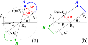
Figure 4: Slow dynamics of the rotor centres. (a) Equal rotors. The mean position $\mathbf{R}$ is at rest and the dynamics involves the relative distance $\mathbf{r}$ only. After a period $T_{0}$, we observe a net rotation of an angle $\Delta\theta$. Here $\sigma_{A}=\sigma_{B}=-1$ (b) Opposite rotors. In this case $\mathbf{R}$ moves and $\mathbf{r}$ on average stays at its initial value. After a period $T_{0}$, there is a net translation of $\mathbf{R}$ along the direction $\hat{\bm{r}}^{\perp}_{0}$. Here $\sigma_{A}=1$.

We consider the intrinsic reference frame described by unit vectors $\hat{\bm{r}}_{0}$, $\hat{\bm{r}}^{\perp}_{0}$ (which are defined in terms of the vectors $\mathbf{R}_{A},\mathbf{R}_{B}$ at $t=0$). They satisfy $\hat{\bm{r}}_{0}\wedge\hat{\bm{r}}^{\perp}_{0}=\hat{\bm{z}}$. The results above can be expressed in terms of the velocity of the centres of each rotor. The slow dynamics of rotor A, can be expressed compactly by the velocity

$$\dot{\mathbf{R}}_{A}(t)=\dfrac{1}{2}\Big{(}\overline{\bm{\omega}_{1}}\wedge\mathbf{r}(t)\Big{)}+\overline{\dot{\mathbf{R}}},$$ (11)

with the corresponding expression for rotor B. This represents either the effect of a net rotation, occurring only when the rotors have equal spins, or a net translation, if they have opposite spins. Since for a pair of equal rotors, $\mathbf{r}$ rotates, it is convenient to use the parametrization $\mathbf{r}(t)=r_{0}\Big{(}\cos\Omega(t)\hat{\bm{r}}_{0}+\sin\Omega(t)\hat{\bm{r}}^{\perp}_{0}\Big{)}$ where $\Omega(t):=\omega_{1}\sigma_{+}t$.

It is interesting to note that symmetry considerations alone indicate that the qualitative nature of the motion of a pair should be independent of the detailed form of rotor [18, 17]. If the separation of the rotors is large compared to their size, the net flow is well approximated by superposing the flow fields generated by the individual rotors. On timescales long compared to the period of the rotation of $\hat{\bm{u}}$, their combined motion can only depend on the two directions $\hat{\bm{r}}_{0}$ and $\hat{\bm{r}}^{\perp}_{0}$ characterising the configuration of the rotors. Moreover, the flow field generated by each rotor has rotational symmetry. From this it follows that any net velocity has no component on the $\hat{\bm{r}}_{0}$ direction. Hence, it can only have a net component along the $\hat{\bm{r}}^{\perp}_{0}$ direction. Implementing this for two identical rotors, one easily sees that their two centres are convected by equal and opposite flows - leading to rotation; while when they have opposite spin they are both subject to the same velocity and translate together. This insight can be very productively combined with analytic techniques to investigate the slow dynamics.

3.3 Comparison with numerics

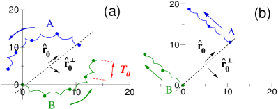
Figure 5: Dynamic trajectories of rotor centres in the plane, obtained from numerical simulations. Continuous lines represent the instantaneous positions of the rotor centres incorporating both ‘slow’ and ‘fast’ motions; solid circles show its slow envelope, at time intervals that are multiples of the period $T_{0}$. (a) Equal rotors with $\sigma_{A}=-1$. The trajectories of the rotors oscillate in the radial direction while performing a revolution around their common centre. The slow dynamics, however, describes a circular trajectory. (b) Opposite rotors, with $\sigma_{A}=1$. The two rotor centres oscillate around the radial direction while moving on average in a direction orthogonal to their separation: the ‘slow’ motion is a straight line in this direction. The initial relative orientation is $\hat{\bm{r}}_{0}=\hat{\bm{x}}+\hat{\bm{y}}$ and the parameters are $l=5\mu$m, $a=0.5\mu$m, $f=10$pN, $L=6\mu$m, $r_{0}=15\mu$m.

We compare analytical results with numerical simulations that involve the full tensorial expression of the hydrodynamic tensor, allowing us to investigate the dynamics of two rotors beyond the regime where $\epsilon\ll 1$. Equations (6) are implemented in C and integrated numerically using the Taylor algorithm [35]. The accuracy of the results can be improved by simply using a smaller integration step $dt$. Here, we have used a time-step $dt=10^{-4}\frac{T_{0}}{4}$. We consider many internal cycles $T_{0}$ and keep track of positions and angles of rotors both i) at each time step (instantaneous) and ii) after a period $T_{0}$. We have checked that a different phase prescription for $\hat{\bm{u}}^{\alpha}$ does not affect the dynamics, which is qualitatively unchanged even in the case of a phase difference between the directors.

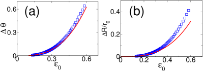
Figure 6: Net changes in a cycle as functions of $\epsilon_{0}$. Approximated analytical results (continuous curves) compared with numerical simulations (squares). (a) Equal rotors. The net angle $|\Delta\theta|$ in a cycle. (b) Opposite rotors. Net displacements $|\Delta R|$ in a cycle, rescaled with the initial separation $r_{0}$. In both cases parameters are the same of figure (5) (except $r_{0}$).

For $\epsilon\ll 1$, results are in quantitative agreement with approximate analytical solutions, with which they are compared in Figure (6) as a function of the initial separation $r_{0}$, at constant $L$. As $\epsilon$ is increased, deviations appear as expected, however the qualitative behaviour remains unchanged. There we plot the net rotation angle after a period $T_{0}$ from simulations and the approximate analytic result given by

$$|\Delta\theta|=T_{0}\omega_{1}=\frac{2\pi l\epsilon^{3}_{0}}{L\,g\left(l/a\right)}$$ (12)

and similarly the net displacement, rescaled with $r_{0}$, compared with the approximate analytic result

$$\left|\frac{\Delta R}{r_{0}}\right|=T_{0}v_{1}=\frac{\pi l\epsilon^{3}_{0}}{L\,g\left(l/a\right)}.$$ (13)

3.4 Comparison to three dimensional hydrodynamics

It is also instructive to consider (briefly) rotors that move in an unbounded three dimensional fluid of viscosity $\eta$. Here rotors are composed of spheres of radius $a$, rather than disks, linked together. We assume that their directors $\hat{\bm{u}}^{\alpha}$ can be confined to two dimensions by some mechanism. The dynamics of point forces $\mathbf{f}=f\sigma\hat{\bm{u}}^{\perp}$ acting on the spheres and lying entirely in that plane can be represented by means of the Oseen tensor [31]: $\bm{H}(\mathbf{r})=\frac{1}{8\pi\eta}\frac{\mathbb{I}+\hat{\bm{r}}\otimes\hat{\bm{r}}}{r}$ for $r\gg a$. The phenomenology that we find is qualitatively similar to rotors moving in a thin film, with only qualitative differences. The centre of a single rotor is at rest and its director $\hat{\bm{u}}$ rotates with a constant angular velocity $\omega^{(3d)}_{0}=\frac{f}{\pi\eta L}(\frac{1}{3a}-\frac{1}{4L})$. Two interacting rotors show again a combination of fast and slow dynamics. The slow motion is a rotation around the common centre for rotors having the same spin, and a net translation for rotors having opposite spin. These slow motions are described again by means of equations that have the same form of eqs (9) and (10), with same directions but different magnitudes. To leading order in $\epsilon$ these magnitudes are $\omega^{(3d)}_{1}=\frac{\epsilon^{3}_{0}f}{4\pi\eta L^{2}}$, for same rotors and $v^{(3d)}_{1}=\frac{1}{2}r_{0}\omega^{(3d)}_{1}$, for opposite rotors.

Similar results can also be obtained also by replacing the model of rotor with a single spinning sphere of radius $b$ with an angular velocity $\bm{\Omega}$ of fixed magnitude, directed along the $\pm\hat{\bm{z}}$ axis. The flow field at distance $r$, generated by a sphere in placed at the origin, is given by [30]

$$\mathbf{v}=\frac{b^{3}}{r^{3}}\bm{\Omega}\wedge\mathbf{r}.$$ (14)

For separations large compared to the sphere radius, the velocities of the two sphere centres can be approximated by superposing the fields generated by each sphere. Hence for rotors of like spin, i.e. $\bm{\Omega}_{A}=\bm{\Omega}_{B}$, the motion of the pair is a rotation about their common centre with angular velocity given by $\frac{1}{2}\mathbf{r}\wedge\mathbf{v}$, with $\mathbf{v}$ the same as in eq (14). In contrast, for opposite spin, each sphere translates in the direction perpendicular to the separation vector $\mathbf{r}$, with a velocity given by (14).

3.5 A pair of rotors as a model swimmer

The dynamical behaviour of two rotors described above suggests a natural application. Since two opposite rotors move in a straight line, they provide a nice model of a self-propeller, whose force density has the form of a torque dipole. The mean propulsion speed depends on the rotor separation and follows from eqn. (13) as $\hat{v}=\Delta R/T_{0}$. The direction of motion can be varied easily by controlling the torques: the motion can be reversed by simultaneously inverting both the torques. The swimmer can be made to change its direction by reversing one of them for a short time since as discussed above, when the two spins have the same value $\sigma=1$ ( $\sigma=-1$) the swimmer will rotate clockwise (counter-clockwise) with an angular displacement (in 1 cycle) given to leading order by eqn. (12).

Taking account of fluctuations will lead to Brownian motion along the direction of the rotor separation with a diffusion constant $D$ proportional to the magnitude of the fluctuations. This means that the speed of the propulsion which will fluctuate around the average $\hat{v}$. As a result, our description will remain valid until the separation of the rotors becomes comparable to rotor size $r_{0}\sim L$, when the rotors strongly interact with each other. This can be used to estimate the lifetime of the rotor-swimmer as a first passage time off a particle diffusing in one dimension [36]. To avoid this, and obtain a permanent swimmer, two rotors could be mechanically linked together a fixed distance apart by a rigid linker [37].

Finally we make some general observations about the properties of this self-propeller. As required by the scallop theorem [38], a low Reynolds number swimmer must undergo cyclic shape deformations that are non-reciprocal requiring at least two degrees of freedom. It is clear that the rotations of the pairs of rotors prescribe a non-reciprocal cyclic motion. So despite being force-free, and torque-free, an assembly made of two rotors can swim, as a result of hydrodynamic interactions. It provides another example of an idealised simple swimmer model [39, 40, 41] that it might be possible to construct on the nanoscale. A possible experimental realisation would be a pump created by dielectric spheres made to rotate by a multi-bead optical trap. It is noteworthy that more complex rotor-swimmers composed of two torque dipoles [17] of opposite sign can also be used to construct an albeit less efficient swimmer [32].

In conclusion, we have investigated analytically and numerically the dynamics of rotors confined to two dimensions by a viscous film (such as a membrane) sandwiched between a less viscous bulk fluid. We first introduced the model of rotor and subsequently studied the interaction between two such rotors. We found that the resulting dynamics depends on the relative spin of the pair and that it involves fast and slow quantities. Concentrating on the slow variables, we find that for opposite rotors the hydrodynamic interactions lead to a net translation of the pair while for like rotors they lead to a relative rotation of the pair around each other. There are a number of possible experimental realisations of this system. For example, qualitative studies of chemically driven ’nano’-rotors have already been performed. A promising direction for future studies is to confine them in thin films giving greater control of their behaviour and allowing a more quantitative study of their interactions. Another natural application is self-locomotion. Two rotors can be used to construct a swimmer: when the torques are equal and opposite, the swimmer translates; when the torques are the same, it can rotate in a controlled way with respect to its original direction, as discussed above. Alternatively, two tethered rotors with opposite spin can generate a net flow along their common axis, while rotors with same spin would generate a flow with rotational symmetry around them. Finally, this study serves as basis and provides a natural framework to describe the collective behaviour of many rotors, that we will address in the future [32].

- [1]
- [2] \NamePedley T. J. Kessler J. O. \REVIEWAnnual Review of Fluid Mechanics241992313.
- [3] \NameWu X. L. Libchaber A. \REVIEWPhys. Rev. Lett.8420003017;
- [4] \NameAditi Simha R. Ramaswamy S. \REVIEWPhys. Rev. Lett.892002058101.
- [5] \NameDomborowski C. et al. \REVIEWPhys. Rev. Lett.932004098103; \NameTuval I. et al. \REVIEWPNAS10220052277.
- [6] \NameToner J. Tu Y. Ramaswamy S.. \REVIEWAnnals of Physics 3182005170.
- [7] \NameDreyfus R. et al. \REVIEWNature4372005862.
- [8] \NameSokolov A. et al. \REVIEWPhys. Rev. Lett.982007158102.
- [9] \Name Saintillan D. Shelley M. J. \REVIEWPhys. Rev. Lett.1002008178103 ; \REVIEWPhysics of Fluids 202008123304 .
- [10] \NamePeruani F., Deutsch A. Bar M. \REVIEWThe European Physical Journal - Special Topics1572008111.
- [11] \NameChaté H. et al. \REVIEWPhys. Rev. E772008046113.
- [12] \NameLeptos K. C. et al. \REVIEWPhys. Rev. Lett.1032009198103.
- [13] \NameGosh A. Fisher P. \REVIEWNano Letters920092243.
- [14] \NameBaskaran A. Marchetti M. C. \REVIEWPNAS 106200915567.
- [15] \NameKruse K., Joanny J.-F., Julicher F., Prost J. Sekimoto K. \REVIEWEur. Phys. J. E 1620055
- [16] \NameAhmadi A., Marchetti M. C., Liverpool T. B. \REVIEWPhys. Rev. E742006061913
- [17] \NameLenz P., Joanny J.-F., Julicher F. Prost J. \REVIEWPhys. Rev. Lett. 912003108104; \REVIEWEur. Phys. J. E 132004379 390.
- [18] \NameLlopis I. Pagonabarraga I. \REVIEWEur. Phys. J. E 262008103 - 113.
- [19] \NameUchida N.Golestanian R. \REVIEWPhys. Rev. Lett. 1042010178103.
- [20] \NameCatchmark J., Subramanian S. Sen A. \REVIEWSmall 12005202.
- [21] \NameDhar P. et al. \REVIEWNano Letters 6200666.
- [22] \Name Riedel I.H., Kruse K., Howard J. \REVIEWScience 3092005300.
- [23] \NameB.A. Grzybowski, et al., \REVIEWProc. Natl. Acad. Sci.9920024147.
- [24] \NameYang Wang et al. \REVIEWJ. Am. Chem. Soc. 13120099926.
- [25] \NameSaffman P. G. Delbruck M. \REVIEWPNAS 7219753111; \NameSaffman P. G. \REVIEWJ. Fluid. Mech.731976593-602.
- [26] \Name Hughes B.A., Pailthorpe B.A. White L.R. \REVIEWJ. Fluid Mech.1101981349–372
- [27] \NameLubensky D. K. Goldstein R. E. \REVIEWPhysics of Fluids 81996843.
- [28] \NameNaji A., Levine A. J. Pincus P. A. \REVIEWBiophysical Journal 93200749.
- [29] \NameLevine A. J., Liverpool T. B. MacKintosh F. \REVIEWPhys. Rev. Lett. 932004038102; \REVIEWPhys. Rev. E692004021503.
- [30] \NameLifshitz E. Landau L. \BookFluid Mechanics 2nd Edition (Pergamon Press, Oxford) 1987.
- [31] \NameDoi M. Edwards S. \BookThe Theory of Polymer Dynamics (Clarendon Press, Oxford) 1988.
- [32] M. Leoni and T.B. Liverpool, unpublished (2010).
- [33] \NamePavliotis G. Stuart A. \BookMultiscale Methods: Averaging and Homogenization (Springer ) 2008.
- [34] \NameSrogatz S. \BookNonlinear dynamics and Chaos (Perseus) 1994.
- [35] \NameLagomarsino M. Cosentino, Jona P. Bassetti B. \REVIEWPhys. Rev. E 682003021908
- [36] \NameRedner S. \BookA guide to first passage problems (Cambridge University Press, Cambridge) 2001.
- [37] \NameLiverpool T. Maggs A.C. \REVIEWMacromolecules3420016064
- [38] \NamePurcell E. M. \REVIEWAmerican J. of Phys.4519773.
- [39] \NameNajafi A. Golestanian R. \REVIEWPhys. Rev. E692004062901; \NameGolestanian R. Ajdari A. \REVIEWPhys. Rev. E772008036308;
- [40] \NameLauga E. Bartolo. D \REVIEWPhys. Rev. E782008030901
- [41] \NameNajafi A. Zargar R. \REVIEWPhys. Rev. E812010067301.