Chiral matter wavefunctions in warped compactifications

Abstract

We analyze the wavefunctions for open strings stretching between intersecting 7-branes in type IIB/F-theory warped compactifications, as a first step in understanding the warped effective field theory of 4d chiral fermions. While in general the equations of motion do not seem to admit a simple analytic solution, we provide a method for solving the wavefunctions in the case of weak warping. The method describes warped zero modes as a perturbative expansion in the unwarped spectrum, the coefficients of the expansion depending on the warping. We perform our analysis with and without the presence of worldvolume fluxes, illustrating the procedure with some examples. Finally, we comment on the warped effective field theory for the modes at the intersection.

1 Introduction

Although string theory is the leading candidate for a quantum theory of gravity, finding realistic models in a string framework is a difficult task. Among the challenges faced by such constructions, as well as by any candidate ultraviolet completion of the Standard Model, is an explanation of the electroweak hierarchy. A virtue of string models is that they typically contain extra dimensions, the existence of which potentially allows the hierarchy problem to be translated into a question of geometry. For example, if the degrees of freedom in the visible sector are realized by open strings localized at D-branes and their intersections, then the hierarchy can in principle result from extra dimensions that are large with respect to the string length ArkaniHamed:1998rs ; *Antoniadis:1998ig; Shiu:1998pa (see also Antoniadis:1990ew ; Lykken:1996fj ). In practice, however, it remains challenging to find compactifications with stabilized moduli that admit such a low string scale and yet are phenomenologically viable (see for example Balasubramanian:2005zx ; *Conlon:2005ki; *Conlon:2006gv).

Another related approach to translating the hierarchy problem into a geometrical problem is warping. In type II string theories and F-theory, D-branes and other extended objects are necessary for the cancellation of tadpoles and providing the open strings required to produce realistic models. The gravitational influence of these ingredients results in a spacetime that is warped in the sense that it cannot be described as a direct product. Additionally, stabilization of the internal geometry requires the addition of fluxes and the back-reaction of such fluxes also leads to warping. If the warping is strong, then the gravitational redshift provides a mechanism for the exponential suppression of the electroweak scale. Although this method of generating the hierarchy was first introduced from a 5d point of view Randall:1999ee , one may also implement this scheme in the context of string theory Verlinde:1999fy ; *Dasgupta:1999ss; *Greene:2000gh; *Becker:1996gj; *Becker:2000rz; *Giddings:2001yu (see Douglas:2006es ; *Blumenhagen:2006ci; *Grana:2005jc for reviews). In addition to providing phenomenologically attractive constructs from the point of view of particle physics, warped geometries have played an important role in string cosmology by providing a framework to describe either inflation Kachru:2003sx (for reviews see Linde:2005dd ; *Cline:2006hu; *Kallosh:2007ig; *Burgess:2007pz; *McAllister:2007bg; *Baumann:2009ni) or late time acceleration Kachru:2003aw . Finally, warped geometries are also key to the understanding of strongly-coupled gauge theories by way of the gauge/gravity correspondence Maldacena:1997re ; *Gubser:1998bc; *Witten:1998qj.

Due to the many applications of warped compactifications in string theory, it is of clear value to understand their dynamics. Although in principle such dynamics follow from worldsheet methods, warped compactification of type II theories necessarily include Ramond-Ramond fluxes and, except in special cases Metsaev:1998it ; *Metsaev:2001bj, it is challenging to quantize string theory in such backgrounds. An alternative method to describe the low energy dynamics is to consider the effective action resulting from a dimensional reduction of the supergravity description of these geometries. However, even when considering only the fields in the 4d supergravity multiplet, deducing such an action has proven to be a subtle problem Giddings:2005ff ; *Frey:2006wv; *Burgess:2006mn; *Douglas:2008jx; *Shiu:2008ry; *Frey:2008xw; *Martucci:2009sf; *Underwood:2010pm. The problem becomes even more involved if one considers compactifications with a realistic gauge sector, as such sectors are localized on the worldvolumes of D-branes, the light degrees of freedom of which are also be affected by the presence of warping Marchesano:2008rg ; Chen:2009zi . An understanding of the warped effective field theory of these open string modes is thus a crucial ingredient in any detailed phenomenological study of warped compactifications.

In Marchesano:2008rg , we considered warped type IIB compactifications and studied the wavefunctions for open strings beginning and ending on the same $\mathrm{D}7$-brane. Such a $\mathrm{D}7$-brane fills the large, non-compact four dimensions and wraps a 4-cycle of the internal geometry. Since the low-energy effective action follows from dimensional reduction to 4d, almost any quantity arises as an overlapping integral of warped wavefunctions, which are in turn computed by solving a warped Dirac or Laplace equation. From our analysis in Marchesano:2008rg , we found that the wavefunctions for the bosonic degrees of freedom remain unmodified by the presence of warping, while the wavefunctions associated with the fermions are modified in a way that is consistent with supersymmetry. In particular, the effect of warping on the fermionic degrees of freedom depends on the chirality of such fermions in the internal $\mathrm{D}7$-brane dimensions. The behavior of the wavefunctions and 4d effective action can then be deduced by the 8d Dirac-Born-Infeld and Chern-Simons action describing the bosonic degrees of freedom, together with the 8d action of Martucci:2005rb describing the fermionic degrees of freedom.

In this work, we extend our analysis in Marchesano:2008rg by analyzing the wavefunctions for open strings stretching between intersecting $\mathrm{D}7$-branes in warped compactifications. Such strings generically give rise to chiral bifundamental fields and are thus of obvious phenomenological interest. The strategy that can be followed to describe such an intersection is to consider the non-Abelian generalization of the $\mathrm{D}7$-brane action describing the low-energy dynamics in the limit where $N$ branes are coincident. The non-trivial intersection can then be described by a varying background profile for the transverse deformations field $\Phi$ of the non-Abelian $\mathrm{D}7$-brane theory, in such a way that the initial gauge group is broken as $\mathrm{U}\left(N\right)\rightarrow\mathrm{U}\left(N_{a}\right)\times\mathrm{U}\left(N_{b}\right)$ by the presence of $\Phi$. Since the energy of a string is proportional to its length, one expects that the massless strings stretching between the intersecting $\mathrm{D}7$-branes are localized at the intersection locus. Indeed, in the unwarped case it is known that the corresponding wavefunctions are exponentially peaked there Katz:1996xe ; Hashimoto:2003xz ; *Nagaoka:2003zn.

Although an intersection of $\mathrm{D}7$-branes is sufficient to obtain bifundamental fields, this does not automatically yield a 4d chiral spectrum. In order to obtain 4d chirality one must either place the intersection at a singularity or to consider intersections that support a non-trivial worldvolume flux $F$. In the latter, more generic case, the Laplace and Dirac equations are modified by the presence of a non-vanishing vector potential $A$, requiring that the wavefunctions at the intersection be modified as well. For instance, if the intersection is a flat two-torus, one can show that the unwarped wavefunctions are constant in the unmagnetized case, while they are described by Riemann $\vartheta$-functions as soon as $F\neq 0$ Cremades:2004wa .

For the adjoint fields studied in Marchesano:2008rg , the warping modification of the open strings wavefunctions could be simply expressed in terms of the warp factor, as these fields have a well-defined chirality in the internal $\mathrm{D}7$-brane dimensions. As the massless fields at the intersection do not have a well-defined internal chirality, the warped wavefunctions no longer take such a simple expression. However, in the weak warping case (i.e., a slowly varying warp factor), the effect of warping can be treated as a perturbation. The wavefunction can then be expanded in terms of the massive modes of the unwarped geometry, and the coefficients characterizing the expansion can be determined using perturbation theory.

Our paper is organized as follows. In section 2, we consider some generalities of intersecting $7$-branes in warped compactifications. Drawing on Butti:2007aq and Myers:1999ps , we propose a non-Abelian generalization of the superpotential and $D$-terms of Jockers:2005zy ; Martucci:2006ij which allow us to extend the supersymmetry conditions of Marino:1999af ; Gomis:2005wc ; Martucci:2005ht to intersecting $\mathrm{D}7$-branes in warped backgrounds. In section 3, we consider the fluctuations about unmagnetized intersections, as a warm-up for the more involved, magnetized case. The equations of motion for these fluctuations follow again by considering the $F$- and $D$-flatness conditions as well as a non-Abelian generalization of the fermionic action of Martucci:2005rb . The massive spectrum in the unwarped case is determined in subsection 3.2 and the expansion of the warped zero mode in terms of the unwarped spectrum is presented in subsection 3.3 with some simple examples worked out in subsection 3.4. We then extend our analysis to the magnetized case in section 4. These results lead us in section 5, to address some issues regarding the 4d warped effective field theory for the chiral modes at the intersection. We draw our conclusions in section 6, while our conventions, some technical details, and a discussion on corrections to the $D$-flatness conditions are left for the appendices.

The effective action for bifundamental fields arising from intersecting $\mathrm{D}$-branes have been considered in many other places in the literature, though the effects of warping, which is our focus here, has not yet been widely explored. Such modes are often considered via the worldsheet as reviewed in Blumenhagen:2005mu ; Blumenhagen:2006ci . Field theory treatments include Hashimoto:2003xz ; Nagaoka:2003zn in the context of brane recombination and Cremades:2004wa for the purpose of calculating Yukawa couplings. The intersections of general $7$-branes were considered in Beasley:2008dc ; Cecotti:2009zf ; Donagi:2008ca ; Font:2009gq ; Conlon:2009qq ; Leontaris:2010zd (see also Conlon:2008qi ), though again in the absence of warping. Finally, in addition to the consideration of warped effective actions referenced above, background fluxes which give rise to warping can have additional influence on the wavefunctions; such effects were considered in Camara:2009xy ; *Camara:2009zz for the open string sector.

2 Intersecting D7s in warped compactifications

Let us consider type IIB superstring on the warped product of $\mathbb{R}^{1,3}\times_{\omega}X_{6}$, where $X_{6}$ a compact six-dimensional manifold. That is, we consider the Einstein frame 10d background metric

$$\mathrm{d}s_{10}^{2}=e^{2a}\eta_{\mu\nu}\mathrm{d}x^{\mu}\mathrm{d}x^{\nu}+e^{-2a}\mathrm{d}\tilde{s}_{6}^{2},\quad\quad\mathrm{d}\tilde{s}_{6}^{2}=\tilde{g}_{mn}\mathrm{d}y^{m}\mathrm{d}y^{n},$$ (1)

where the warp factor $e^{-4a}$ varies over $X_{6}$. Such a geometry is supported by the RR $5$-form field strength Verlinde:1999fy ; Giddings:2001yu

$$F_{5}=\bigl{(}1+\ast_{10}\bigr{)}F_{5}^{\mathrm{ext}},\qquad F_{5}^{\mathrm{int}}=\tilde{\ast}_{6}\mathrm{d}e^{-4a}$$ (2)

where $\mathrm{d}\mathrm{vol}_{\mathbb{R}^{1,3}}$ is the volume element of $\mathbb{R}^{1,3}$ and $\ast_{10}$ is the Hodge-$\ast$ built from the warped metric (1) and $\tilde{\ast}_{6}$ is the Hodge-$\ast$ built from $\tilde{g}$. Such $5$-form flux is sourced by objects with finite $\mathrm{D}3$-brane charge such as $\mathrm{D}3$-branes, $\mathrm{O}3$-planes, magnetized $7$-branes and $3$-form flux $G_{3}$. Focusing on supersymmetric warped compactifications requires that $G_{3}$ is a primitive $\left(2,1\right)$-form, $\tilde{g}$ is Kähler and the axio-dilaton $\tau$ is a holomorphic function on $X_{6}$ Grana:2000jj ; *Gubser:2000vg; *Grana:2001xn, so that the elliptic fibration over $X_{6}$ specified by $\tau$ is a Calabi-Yau four-fold. The divisors $\mathcal{S}\subset X_{6}$ on which the fiber degenerates correspond to the location of $7$-branes with the corresponding gauge group $G_{\mathcal{S}}$ Vafa:1996xn ; *Morrison:1996na; *Morrison:1996pp.

Our primary interest in this paper will be on the intersection of two of these divisors where the symmetry further enhances. Localized along this matter curve are additional degrees of freedom that are charged under $G_{\mathcal{S}}\times G_{\mathcal{S}^{\prime}}$ and generalize the well-known bifundamental fields appearing in the low energy spectrum of intersecting $\mathrm{D}7$-branes Bershadsky:1996nh ; Katz:1996xe . For a single stack of $\left(p,q\right)$ $7$-branes, the effective action is given by an $\mathrm{SL}\bigl{(}2,\mathbb{Z}\bigr{)}$ rotation of the usual Dirac-Born-Infeld and Chern-Simons actions, as such branes are simply Dirichlet branes for $\left(p,q\right)$-strings. An intersection of two $\left(p,q\right)$ $7$-branes can then be described by Higgsing this low energy theory, just like the intersection of two $\mathrm{D}7$-branes. Finally, the intersection of a stack of $\left(p,q\right)$ with $\left(p^{\prime},q^{\prime}\right)$ $7$-branes with $\left(p,q\right)\neq\left(p^{\prime},q^{\prime}\right)$ can be treated, following Beasley:2008dc , by means of a topologically twisted YM 8d action with an exceptional gauge group, also Higgsed down to describe the massless modes on a matter curve.

While the latter strategy allows to describe the fields as the $7$-brane intersection in terms of wavefunctions, it is a priori not obvious how to include the effects of warping in this topologically twisted 8d action. In this sense, it seems more reliable to consider an intersection of two $\mathrm{D}7$-branes and make use of the non-Abelian DBI and CS actions, as well as their fermionic counterpart, in order to derive the warped equations of motion for bosonic and fermionic degrees of freedom. Such computations (performed in appendix B and next section, respectively), will however not be our main strategy to derive the warped equations of motion. Instead, we will take a different approach based on the supersymmetry conditions for a stack of $\mathrm{D}7$-branes in a general type IIB background, conditions which we will derive in the remainder of this section.

As we will see, this last approach allows to consider general closed string backgrounds in a rather simple way. Indeed, while we turn off background $3$-form fluxes in our computation, we allow for a varying dilaton and hence a non-Calabi-Yau geometry for the internal space $X_{6}$. This, together with the fact that the BPS equations for a $\mathrm{D}7$-brane and a $(p,q)$ $7$-brane are identical, leads us to believe that our warped equations of motion apply to the more general $\left(p,q\right)$-$\left(p^{\prime},q^{\prime}\right)$ $7$-brane intersection that are of main interest in local F-theory GUT models. It would be interesting to check from first principles if this is indeed the case.

In order to derive the non-Abelian BPS equations, let us first consider a single $\mathrm{D}7$-brane wrapping a $4$-cycle $\mathcal{S}_{4}\subset X_{6}$. The massless open string excitations of this D-brane consist of a gauge field $A$ living on the 8d worldvolume and its transverse fluctuations of its embedding $\Phi^{i}=\lambda^{-1}X^{i}$, where $\lambda=2\pi\alpha^{\prime}$. The $\mathrm{D}7$ will be supersymmetric if Marino:1999af ; Gomis:2005wc ; Martucci:2005ht

1. $\mathcal{S}_{4}$ is holomorphically embedded into $X_{6}$, and

2. the worldvolume field strength $F_{2}=\mathrm{d}A$ satisfies the self-duality condition

   $$\ast_{4}F_{2}=F_{2},$$ (3)

   where $\ast_{4}$ is the Hodge-$\ast$ on $\mathcal{S}_{4}$ built from the induced metric.

These conditions follow from consideration of an effective potential resulting from the superpotential and $D$-term Jockers:2005zy ; Martucci:2006ij .

$$W= \int_{\Sigma_{5}}e^{3\alpha}(\mathrm{Im}\,\tau)^{-1/2}\,P\bigl{[}\Psi_{2}\wedge e^{B_{2}}\bigr{]}\wedge e^{\lambda F_{2}},$$ (4a)

$$D= \int_{\mathcal{S}_{4}}e^{2\alpha}\,P\bigl{[}\mathrm{Im}\,\Psi_{1}\,\wedge e^{B_{2}}\bigr{]}\wedge e^{\lambda F_{2}},$$ (4b)

in which $B_{2}$ is the NS-NS $2$-form, $\tau$ is the axio-dilaton, $P$ indicates the pullback to $\mathcal{S}_{4}$, and $\Sigma_{5}$ is a $5$-chain whose boundaries are $\mathcal{S}_{4}$ and its deformation. Finally, $\alpha$ is related to the Einstein frame warp factor $a$ through

$$\alpha=a+\frac{1}{4}\log\left(\mathrm{Im}\,\tau\right).$$ (5)

As it will turn out, the equations of motion will be written naturally in terms of $\alpha$, and so for simplicity we will often refer to $e^{-4\alpha}$ as the warp factor. The pure spinors $\Psi_{1}$ and $\Psi_{2}$ are given in terms of the warped Kähler form $J=e^{-2\alpha}J_{X_{6}}$ and the (unwarped) fundamental $3$-form of $X_{6}$ by $\Psi_{1}=e^{iJ}$ and $\Psi_{2}=e^{-3\alpha}\Omega_{X_{6}}$. Demanding $F$-flatness implies that $\mathcal{S}_{4}$ is holomorphic and that $F_{2}$ is $\left(1,1\right)$ while demanding $D$-flatness to leading order in $\alpha^{\prime}$ implies that $F_{2}$ is a primitive in $\mathcal{S}_{4}$; together, these two conditions on $F_{2}$ imply that it is self-dual.

Interestingly, the expressions (4) for $W$ and $D$ allow for a simple generalization to the non-Abelian case, following some observations made in Butti:2007aq . To this end, we locally write

$$e^{3\alpha}\left(\mathrm{Im}\,\tau\right)^{-1/2}\,\Psi_{2}\wedge e^{B_{2}}=\mathrm{d}\gamma.$$ (6)

The superpotential and $D$-term can then be expressed as

$$W=\int_{\mathcal{S}_{4}}P\bigl{[}\gamma\bigr{]}\wedge e^{\lambda F_{2}},\quad D=\int_{\mathcal{S}_{4}}P\bigl{[}\mathrm{Im}\,\eta\,\bigr{]}\wedge e^{\lambda F_{2}},$$ (7)

where

$$\eta=e^{2\alpha}\,\Psi_{1}\wedge e^{B_{2}}.$$ (8)

Now, as observed in Appendix A of Butti:2007aq , these expressions take the same form as the Chern-Simons action for a $\mathrm{D}$-brane

$$S_{\mathrm{D}p}^{\mathrm{CS}}=\int_{\mathcal{W}}P\bigl{[}\mathcal{C}\wedge e^{B_{2}}\bigr{]}\wedge e^{\lambda F_{2}},$$ (9)

where $\mathcal{C}$ is the formal sum of R-R potentials and $\mathcal{W}$ is the worldvolume of the brane. Following Myers:1999ps , the non-Abelian generalization of (9) is then given by

$$S_{\mathrm{D}p}^{\mathrm{CS}}=\int_{\mathcal{W}}\mathrm{Str}\biggl{\{}P\bigl{[}e^{i\lambda\iota_{\Phi}\iota_{\Phi}}\mathcal{C}\wedge e^{B_{2}}\bigr{]}\wedge e^{\lambda F_{2}}\biggr{\}},$$ (10)

where, as detailed in Appendix B, $\mathrm{Str}$ indicates a symmetrized trace and $\iota_{\Phi}$ stands for the interior product. The transverse fluctuations are then promoted to adjoint-valued scalars $\Phi$ and the field strength to $F_{2}=\bigl{(}\mathrm{d}-iA\wedge\bigr{)}A$. Finally, the non-Abelian pullback replaces derivatives with gauge covariant derivatives

$$P\left[v\right]_{\alpha}=v_{\alpha}+\lambda v_{i}D_{\alpha}\Phi^{i},$$ (11)

where $D_{\alpha}=\partial_{\alpha}-i\left[A_{\alpha},\cdot\right]$.

Making use of the fact that the pure spinors $\Psi_{1}$ and $\Psi_{2}$ transform under T-duality in a way that is analogous to $\mathcal{C}$, one can then deduce that the non-Abelian superpotential and $D$-term are given by Butti:2007aq

$$W=\int_{\mathcal{S}_{4}}\mathrm{Str}\biggl{\{}P\bigl{[}e^{i\lambda\iota_{\Phi}\iota_{\Phi}}\gamma\bigr{]}\wedge e^{\lambda F_{2}}\biggr{\}},$$ (12a)

and

$$D=\int_{\mathcal{S}_{4}}\mathrm{S}\biggl{\{}P\bigl{[}e^{i\lambda\iota_{\Phi}\iota_{\Phi}}\mathrm{Im}\,\eta\bigr{]}\wedge e^{\lambda F_{2}}\biggr{\}},$$ (12b)

where in the latter $\mathrm{S}$ indicates the symmetrization prescription of Myers:1999ps without taking the trace.

In order to extract the F-term and D-term conditions from (12) it is useful to consider a neighborhood of the internal space $X_{6}$ around $\mathcal{S}_{4}$ such that $(\mathrm{Im}\,\tau)^{-1/2}\Omega_{X_{6}}=\mathrm{d}z^{1}\wedge\mathrm{d}z^{2}\wedge\mathrm{d}z^{3}$ with

$$\mathrm{d}z^{m}=\mathrm{d}y^{m}+\tau_{m}\mathrm{d}y^{m+3},$$ (13)

and the warped Kähler form is given by

$$J=e^{-2\alpha}\frac{i\alpha^{\prime}}{2}\sum_{m=1}^{3}\left(2\pi R_{m}\right)^{2}\mathrm{d}z^{m}\wedge\mathrm{d}\bar{z}^{\bar{m}}.$$ (14)

Moreover, let us consider a local coordinate system such that the complex 4-cycle $\mathcal{S}_{4}$ is parameterized by $(z^{1},z^{2})$, as is usual in the literature of local F-theory models. Then, in absence of background 3-form fluxes we can take $\gamma=z^{3}\mathrm{d}z^{1}\wedge\mathrm{d}z^{2}$, so that $\gamma$ is globally well-defined on $\mathcal{S}_{4}$ and satisfies $\iota_{\Phi}\gamma=0$. The resulting superpotential takes the form

$$W=-\lambda\int_{\mathcal{S}_{4}}\mathrm{d}^{4}z\,\mathrm{Str}\biggl{\{}\Phi F_{\bar{1}\bar{2}}\biggr{\}},$$ (15)

where $\Phi$ is the complexified transverse fluctuation. Demanding $F$-flatness in the $\Phi$ direction immediately gives $F_{\bar{1}\bar{2}}=0$ implying

$$F^{\left(0,2\right)}=F^{\left(2,0\right)}=0.$$ (16)

Likewise, variation with respect to $A$ gives

$$D_{\bar{m}}\Phi=0.$$ (17)

Both of these $F$-flatness conditions are what one would expect from their Abelian counterparts and, while derived in the type IIB framework, they have a simple generalization to F-theory.

Consider now the $D$-flatness condition $D=0$. First we note that since the $\mathrm{D}7$-brane is a real codimension $2$ object, $\iota_{\Phi}^{3}=0$ and so

$$e^{i\lambda\iota_{\Phi}\iota_{\Phi}}=1+i\lambda\iota_{\Phi}\iota_{\Phi}.$$ (18)

It follows then that the non-Abelian $D$-term reads

$$D=\int_{\mathcal{S}_{4}}\mathrm{S}\biggl{\{}e^{2\alpha}\biggl{(}\lambda P\bigl{[}J\bigr{]}\wedge F_{2}-\frac{i\lambda}{6}P\bigl{[}\iota_{\Phi}\iota_{\Phi}J^{3}\bigr{]}+\frac{i\lambda^{3}}{2}P\bigl{[}\iota_{\Phi}\iota_{\Phi}J\bigr{]}\wedge F_{2}\wedge F_{2}\biggr{)}\biggr{\}}$$ (19)

with $\alpha$ a modified warp factor defined as in (14).

In the next section and in Appendix B we will compare the equations of motion that result from the above $F$-flatness and $D$-flatness conditions to those derived from a DBI$+$CS action and its fermionic counterpart valid to leading order in $\alpha^{\prime}$. For such comparison we need to truncate $D$ at order $\lambda$

$$D=\lambda\int_{\mathcal{S}_{4}}\mathrm{S}\biggl{\{}e^{2\alpha}\biggl{(}P\bigl{[}J\bigr{]}\wedge F_{2}-\frac{i}{6}P\bigl{[}\iota_{\Phi}\iota_{\Phi}J^{3}\bigr{]}\biggr{)}\biggr{\}}.$$ (20)

Then, defining the warped fundamental form on $\mathcal{S}_{4}$ as

$$\mathfrak{J}=J\mid_{\mathcal{S}_{4}}=e^{-2\alpha}\frac{i\alpha^{\prime}}{2}\sum_{m=1}^{2}\left(2\pi R_{m}\right)^{2}\mathrm{d}z^{m}\wedge\mathrm{d}\bar{z}^{\bar{m}},$$ (21)

we have that $P\left[J\right]=\mathfrak{J}+\mathcal{O}\left(\lambda^{2}\right)$. Finally, it is also straightforward to show that

$$\frac{1}{6}\iota_{\Phi}\iota_{\Phi}J^{3}=e^{-2\alpha}\frac{i\lambda}{4}\left(2\pi R_{3}^{2}\right)\bigl{[}\Phi,\bar{\Phi}\bigr{]}\mathfrak{J}^{2},$$ (22)

and so

$$D=\lambda\int_{\mathcal{S}_{4}}\mathrm{S}\biggl{\{}e^{2\alpha}\mathfrak{J}\wedge F_{2}+\frac{\lambda}{4}\left(2\pi R_{3}^{2}\right)\mathfrak{J}^{2}\bigl{[}\Phi,\bar{\Phi}\bigr{]}\biggr{\}}.$$ (23)

The symmetrization in this case is trivial and so the $D$-flatness condition is

$$e^{2\alpha}\mathfrak{J}\wedge F_{2}+\frac{\lambda}{4}\left(2\pi R_{3}^{2}\right)\mathfrak{J}^{2}\bigl{[}\Phi,\bar{\Phi}\bigr{]}=0,$$ (24)

which is the expression we will work with from now on. The effect of higher $\alpha^{\prime}$ terms can be included as discussed in Appendix C. Note that the second term in (24) is not to be interpreted as an $\alpha^{\prime}$-correction to the primitivity condition but is instead a modification resulting from taking into account the non-Abelian effects; the factor of $\lambda$ appears because in (14), we have taken $R_{3}$ and $z^{n}$ to be dimensionless. When going from (23) to (24), we have ignored the non-Abelian nature of the warping $\alpha$. That is, by the general prescription of non-Abelian pull-backs on $\mathcal{S}_{4}$, $\alpha$ and other closed-string fields should be interpreted as a functional of the non-Abelian field $\Phi$. As we discuss below, for the case of intersecting $\mathrm{D}7$-branes, treating $\alpha$ as proportional to the identity corresponds to taking the limit of small intersecting angles, and the case of arbitrary angles amounts to a redefinition of $\alpha$.

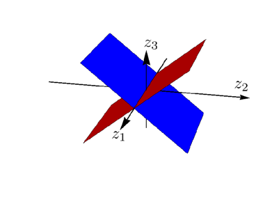
Figure 1: Local view of the intersection of $\mathrm{D}7$-branes described by (27).

Let us now consider the intersection of two stacks of $\mathrm{D}7$-branes. Although our expressions for the superpotential and $D$-term are in principle defined as an integral over a single 4-cycle $\mathcal{S}_{4}$, we can consider $\mathrm{D}7$-branes wrapping different cycles by giving a non-constant vev to the transverse scalar $\Phi$, such that the initial worldvolume gauge theory is Higgsed as $\mathrm{U}\left(N\right)\rightarrow\mathrm{U}\left(N_{a}\right)\times\mathrm{U}\left(N_{b}\right)$ by the presence of $\langle\Phi\rangle$. This vev can be taken to be

$$\left\langle\Phi\right\rangle=\Delta=\begin{pmatrix}\Delta_{a}\mathbb{I}_{N_{a}}&\\ &\Delta_{b}\mathbb{I}_{N_{b}}\end{pmatrix},$$ (25)

where $\Delta_{a,b}$ are holomorphic functions of $z^{1},z^{2}$, so that the F-flatness condition (17) is satisfied at the level of the background. Note that this choice satisfies $\bigl{[}\Delta,\bar{\Delta}\bigr{]}=0$, so setting $F_{2}=0$ is consistent with supersymmetry. Geometrically, (25) describes a stack of $N_{a}$ $\mathrm{D}7$-branes wrapping the $4$-cycle specified by $z^{3}=\lambda\Delta_{a}$ and a stack of $N_{b}$ $\mathrm{D}7$-branes wrapping the $4$-cycle $z^{3}=\lambda\Delta_{b}$, thus intersecting at the complex curve $\Sigma=\Delta_{a}\cap\Delta_{b}\subset\mathcal{S}_{4}$.

Given this background for $\Phi$, the spectrum of open string modes arises from fluctuations around it such as

$$\delta\Phi=\begin{pmatrix}\phi^{a}&\phi^{-}\\ \phi^{+}&\phi^{b}\end{pmatrix}.$$ (26)

The block diagonal fluctuations $\phi^{a,b}$ correspond to strings beginning and ending on the same stack, while the $\phi^{\mp}$ fluctuations correspond to strings stretching from one stack to the other, giving the charges shown in Table 1. If $\Delta_{a}=\Delta_{b}$ has no solution (e.g., if $\Delta_{a}-\Delta_{b}$ is constant) then all the modes arising from $\phi^{\mp}$ are necessarily massive. However, if the branes do intersect, then $\phi^{\mp}$ will (partially) describe the massless bifundamental fields localized at the intersection. Because the string tension is proportional to its length, for intersecting $\mathrm{D}7$-branes the massless modes of $\phi^{\mp}$ should be localized around the points of intersection. Therefore, to capture the dynamics of these fields it suffices to approximate $\Delta_{a,b}$ by linear functions (see Fig. 1)

$$\Delta=\begin{pmatrix}M_{3}^{\left(a\right)}\lambda^{-1}\mathbb{I}_{N_{a}}z^{2}&\\ &M_{3}^{\left(b\right)}\lambda^{-1}\mathbb{I}_{N_{b}}z^{2}\end{pmatrix}.$$ (27)

so that the intersection curve is given by $z_{2}=z_{3}=0$ and the intersection is described by an $\mathrm{SU}\left(2\right)$ rotation on the $z^{2}$-$z^{3}$ plane, in agreement with the results of Berkooz:1996km . In the following we will take $M_{3}^{\left(a\right)}>M_{3}^{\left(b\right)}$ though there are no significant changes if we flip the inequality.

field	$\mathrm{U}\left(N_{a}\right)$	$\mathrm{U}\left(N_{b}\right)$
$\phi^{a}$	$\mathbf{adj}$	$\mathbf{1}$
$\phi^{b}$	$\mathbf{1}$	$\mathbf{adj}$
$\phi^{-}$	$\square$	$\overline{\square}$
$\phi^{+}$	$\overline{\square}$	$\square$

Table 1: Charges for the fields in (26).

As mentioned above, the non-Abelian $D$-flatness conditions are derived by essentially neglecting the dependence of bulk fields on $\Phi$. That is, in general a bulk field $\Psi$ should be interpreted as a functional of the adjoint-valued transverse fluctuations Myers:1999ps

$$\Psi\bigl{[}\Phi\bigr{]}=\sum_{n=0}^{\infty}\lambda^{n}\Phi^{i_{1}}\cdots\Phi^{i_{n}}\Psi_{i_{1}\ldots i_{n}}.$$ (28)

While higher powers of $\Phi$ contain higher powers of $\alpha^{\prime}$, $\langle\Phi\rangle=\Delta$ contains a factor of $\lambda^{-1}$ via  (27) and so, schematically, at the level of the background we have

$$\Psi\sim\sum_{n=0}^{\infty}\left(M_{3}^{\left(a,b\right)}\right)^{n}\Psi_{n}\bigl{(}z^{2},\bar{z}^{\overline{2}}\bigr{)}.$$ (29)

Therefore, neglecting higher terms in the expansion (28) is reliable in the limit where $M_{3}^{\left(a,b\right)}$ (that is, the intersection angles), are small. Nevertheless, as shown in Appendix C, taking into account the full non-Abelian pull-back (28) does not modify the form of the non-Abelian $D$-term equation, and all the corrections can be absorbed in a redefinition of the warping $\alpha$.

Finally, in order to have a 4d chiral spectrum, the intersection curve must support a non-vanishing magnetic flux Manton:1981es ; *Chapline:1982wy; *RandjbarDaemi:1982hi; *Wetterich:1982ed; *Frampton:1984px; *Frampton:1984pk; *Witten:1983ux; *Witten:1984dg; *Pilch:1984ur; *Pilch:1985pm. As $[\Delta,\bar{\Delta}]=0$ the $F$-term (16) and the truncated $D$-term (24) conditions require that $F_{2}$ is self-dual, just as in the Abelian case. Let us for simplicity choose a magnetic flux that does not further break down the gauge group, such as

$$\langle F_{2}\rangle=\sum_{m=1}^{2}\frac{\pi i}{\mathrm{Im}\,\tau_{m}}\begin{pmatrix}M^{\left(a\right)}_{m}\mathbb{I}_{N_{a}}&\\ &M^{\left(b\right)}_{m}\mathbb{I}_{N_{b}}\end{pmatrix}\mathrm{d}z^{m}\wedge\mathrm{d}\bar{z}^{\bar{m}}.$$ (30)

Imposing self-duality then amounts to satisfying the condition

$$\frac{M_{1}^{\left(a,b\right)}}{\mathcal{V}_{1}}+\frac{M_{2}^{\left(a,b\right)}}{\mathcal{V}_{2}}=0,\quad\quad\mathcal{V}_{m}=\left(2\pi R_{m}\right)^{2}\mathrm{Im}\,\tau_{m}.$$ (31)

3 Unmagnetized intersections

Given the $\mathrm{D}7$-brane supersymmetry conditions derived in the previous section, the equations of motion for the open string zero modes can be obtained by expanding these BPS conditions to first order in fluctuations. In the following, we will apply this observation to analyze the zero modes at the intersection of two unmagnetized stacks of $\mathrm{D}7$-branes. Notice that such intersection, unless placed at a singularity, will yield a non-chiral 4d spectrum upon dimensional reduction. Nevertheless, this simple case already demonstrates the non-trivial effect that warping has on open strings at $\mathrm{D}7$-brane intersections, and will serve as a useful warmup for the more general magnetized case.

3.1 Equations of motion

Open strings localized at the intersection correspond to bifundamental fluctuations around the vev (27) and $\langle F_{2}\rangle=0$. Since this open string background is supersymmetric, the zero mode fluctuations should also satisfy the BPS conditions (16), (17), and (24). Let us write these fluctuations as

$$A_{m}=\sqrt{2\pi}R_{m}a_{m},\qquad\Phi=\Delta+\frac{2}{\sqrt{2\pi}R_{3}\lambda}\phi,$$ (32)

where $\Delta$ is given in (27). We are interested only in the bifundamental fluctuations so we take

$$a_{m}=\begin{pmatrix}0&\bigl{(}\phi^{+}_{m}\bigr{)}^{\dagger}\\ \bigl{(}\phi^{-}_{m}\bigr{)}^{\dagger}&0\end{pmatrix},\qquad\phi=\begin{pmatrix}0&\phi_{3}^{-}\\ \phi^{+}_{3}&0\end{pmatrix},$$ (33)

so that we then have

$$\bar{a}_{\overline{m}}=\begin{pmatrix}0&\phi^{-}_{m}\\ \phi^{+}_{m}&0\end{pmatrix},\qquad\bar{\phi}=\begin{pmatrix}0&\left(\phi^{+}_{3}\right)^{\dagger}\\ \left(\phi^{-}_{3}\right)^{\dagger}&0\end{pmatrix}.$$ (34)

The labeling of the fluctuations and prefactors are introduced for latter convenience, as upon dimensional reduction $\bar{a}_{\bar{m}}$ and $\phi$ correspond to the bosonic d.o.f. of the left-handed 4d chiral multiplets, and ${a}_{m}$ and $\bar{\phi}$ to its CPT conjugates.

Plugging (32) back into the BPS conditions of the previous section and expanding them up to linear order in fluctuations, we obtain the equations of motion for $\bar{a}_{\bar{m}}$ and $\phi$. In particular, the F-term condition $F^{\left(0,2\right)}=0$ reads

$$F_{\bar{1}\bar{2}}=2\pi R_{1}R_{2}\begin{pmatrix}0&\hat{\partial}_{1}^{\ast}\phi^{-}_{2}-\hat{\partial}_{2}^{\ast}\phi^{-}_{1}\\ \hat{\partial}_{1}^{\ast}\phi^{+}_{2}-\hat{\partial}_{2}^{\ast}\phi^{+}_{1}&0\end{pmatrix}=0,$$ (35)

where we have defined

$$\hat{\partial}_{m}=\frac{1}{\sqrt{2\pi}R_{m}}\partial_{m}.$$ (36)

The F-term condition $D_{\bar{m}}\Phi=0$ gives

$$D_{\bar{m}}\Phi= \frac{2}{\sqrt{2\pi}R_{3}\lambda}\partial_{\bar{m}}\phi-i\sqrt{2\pi}R_{m}\bigl{[}\bar{a}_{\overline{m}},\Delta\bigr{]}$$

$$= \frac{2R_{m}}{R_{3}\lambda}\begin{pmatrix}0&\hat{\partial}_{m}^{\ast}\phi^{-}_{3}+\frac{i}{2}\sqrt{2\pi}R_{3}{2}I_{3}^{\left(ab\right)}z^{2}\phi_{m}^{-}\\ \hat{\partial}_{m}^{\ast}\phi^{+}_{3}-\frac{i}{2}\sqrt{2\pi}R_{3}I_{3}^{\left(ab\right)}z^{2}\phi^{+}_{m}&0\end{pmatrix}=0,$$ (37)

where we have defined

$$I_{3}^{\left(ab\right)}=M_{3}^{\left(a\right)}-M_{3}^{\left(b\right)}.$$ (38)

Finally, for the $D$-flatness condition (24), we use the fact that

$$\mathfrak{J}\wedge F_{2}=e^{-2\alpha}\frac{i\alpha^{\prime}}{2}\biggl{\{}\bigl{(}2\pi R_{1}\bigr{)}^{2}F_{2\bar{2}}+\bigl{(}2\pi R_{2}\bigr{)}^{2}F_{1\bar{1}}\biggr{\}}\mathrm{d}^{4}z$$ (39)

so that in terms of fluctuations around $\langle F_{2}\rangle=0$, (24) becomes

$$0=\frac{i\alpha^{\prime}}{2}\biggl{\{} \sum_{m=1}^{2}\begin{pmatrix}0&\hat{\partial}_{m}\phi_{m}^{-}-\hat{\partial}_{m}^{\ast}\bigl{(}\phi_{m}^{+}\bigr{)}^{\dagger}\\ \hat{\partial}_{m}\phi_{m}^{+}-\hat{\partial}_{m}^{\ast}\bigl{(}\phi_{m}^{-}\bigr{)}^{\dagger}&0\end{pmatrix}$$

$$-e^{-4\alpha}\frac{i}{2}\sqrt{2\pi}R_{3}I_{3}^{\left(ab\right)}\begin{pmatrix}0&\bar{z}^{\bar{2}}\phi_{3}^{-}-z^{2}\bigl{(}\phi^{+}_{3}\bigr{)}^{\dagger}\\ -\bar{z}^{\bar{2}}\phi_{3}^{+}+z^{2}\bigl{(}\phi^{-}_{3}\bigr{)}^{\dagger}&0\end{pmatrix}\biggr{\}}.$$ (40)

To sum up, the conditions for $F$ and $D$-flatness on the $\mathrm{D}7$-brane bosonic fluctuations are

$$0= \bigl{(}\hat{D}_{1}^{\pm}\bigr{)}^{\dagger}\phi^{\mp}_{2}-\bigl{(}\hat{D}_{2}^{\pm}\bigr{)}^{\dagger}\phi^{\mp}_{1},$$ (41a)

$$0= \bigl{(}\hat{D}_{2}^{\pm}\bigr{)}^{\dagger}\phi_{3}^{\mp}-\bigl{(}\hat{D}^{\pm}_{3}\bigr{)}^{\dagger}\phi_{2}^{\mp},$$ (41b)

$$0= \bigl{(}\hat{D}_{3}^{\pm}\bigr{)}^{\dagger}\phi^{\mp}_{1}-\bigl{(}\hat{D}_{1}^{\pm}\bigr{)}^{\dagger}\phi^{\mp}_{3},$$ (41c)

$$0= \hat{D}_{1}^{\mp}\phi^{\mp}_{1}+\hat{D}_{2}^{\mp}\phi^{\mp}_{2}+e^{-4\alpha}\hat{D}_{3}^{\mp}\phi^{\mp}_{3},$$ (41d)

where we have defined the operators

$$\hat{D}_{1,2}^{\mp}=\hat{\partial}_{1,2},\qquad\hat{D}_{3}^{\mp}=\mp\frac{i}{2}\sqrt{2\pi}R_{3}I_{3}^{\left(ab\right)}\bar{z}^{\bar{2}}.$$ (42)

This notation is motivated by the T-dual picture of magnetized $\mathrm{D}9$-branes, in which the intersection angle between $\mathrm{D}7$-branes becomes a magnetic flux (see afim for more details). In the $\mathrm{D}9$-brane picture, $\hat{D}_{m}^{\mp}$ are nothing but the set of normalized covariant derivatives that appear in the (unwarped) Laplace and Dirac operators after assuming that the wavefunctions do not depend on the $(z^{3},\bar{z}^{\bar{3}})$ coordinates and so $\partial_{3}=0$. As we show in Appendix B, the eom resulting from the DBI and CS actions are satisfied whenever eqs.(41) are satisfied.

In the absence of warping, (41) are straightforward to solve. Indeed, the $F$-term equations (41a)-(41c) are solved by taking the ansatz

$$\phi_{m}^{\mp}=\bigl{(}\hat{D}_{m}^{\pm}\bigr{)}^{\dagger}f^{\mp}$$ (43)

for some arbitrary functions $f^{\pm}$. Then for $e^{-4\alpha}=1$, the $D$-term equation (41d) becomes

$$\biggl{\{}\hat{D}_{1}^{\mp}\bigl{(}\hat{D}_{1}^{\pm}\bigr{)}^{\dagger}+\hat{D}_{2}^{\mp}\bigl{(}\hat{D}_{2}^{\pm}\bigr{)}^{\dagger}+\hat{D}_{3}^{\mp}\bigl{(}\hat{D}_{3}^{\pm}\bigr{)}^{\dagger}\biggr{\}}f^{\mp}=0.$$ (44)

As (44) only depends on the intersection coordinates $(z^{1},\bar{z}^{\bar{1}})$ through derivatives, one expects the zero modes to be independent of them. In particular, if we take the ansatz

$$f^{\mp}=\frac{1}{z^{2}}g^{\mp}\bigl{(}\bigl{|}z^{2}\bigr{|}^{2}\bigr{)},$$ (45)

we find the solution to (44) to be Katz:1996xe ; Hashimoto:2003xz ; Nagaoka:2003zn

$$g^{\mp}=e^{-\kappa\left|z^{2}\right|^{2}},\quad\kappa=\frac{1}{2}2\pi R_{2}R_{3}I_{3}^{\left(ab\right)},$$ (46)

giving

$$\phi_{1}^{\mp}=0,\quad\phi_{2}^{\mp}=-\frac{\kappa}{\sqrt{2\pi}R_{2}}\sigma^{\mp}\left(x^{\mu}\right)e^{-\kappa\left|z^{2}\right|^{2}},\quad\phi^{\mp}_{3}=\mp\frac{i\kappa}{\sqrt{2\pi}R_{2}}\sigma^{\mp}\left(x^{\mu}\right)e^{-\kappa\left|z^{2}\right|^{2}},$$ (47)

where we have introduced the function $\sigma^{\mp}$ that depends on the external coordinates $x^{\mu}$ and carries (suppressed) bifundamental gauge indices. Note that as a consequence of the ansatz (43) the same function $\sigma^{\mp}$ appears in both $\phi_{2}^{\mp}$ and $\phi_{3}^{\mp}$. We then conclude that at the intersection there are only two independent complex scalar fields, one transforming under a bifundamental representation of $\mathrm{U}\left(N_{a}\right)\times\mathrm{U}\left(N_{b}\right)$ and the other transforming under the conjugate representation. The other linearly independent solution to (44) is $g^{\mp}=\exp\left(\kappa\left|z^{2}\right|^{2}\right)$ which is not peaked at the intersection and so is discarded when we consider normalizable modes. Finally, note that the space transverse to the matter curve is in general compact, and so one may wonder wether the wavefunctions ought to satisfy some periodicity conditions; however, since we expect the wavefunctions to be highly peaked around the intersection (as the above Gaussian solutions show) such constraints can be safely neglected in our analysis.

Let us now consider the case of non-trivial warping. As one would expect from holomorphicity of the superpotential, the $F$-term equations remain unmodified, so one may again consider the ansatz (43). Plugging it into the warped $D$-term equation gives

$$\biggl{\{}\hat{D}_{1}^{\mp}\bigl{(}\hat{D}_{1}^{\pm}\bigr{)}^{\dagger}+\hat{D}_{2}^{\mp}\bigl{(}\hat{D}_{2}^{\pm}\bigr{)}^{\dagger}+e^{-4\alpha}\hat{D}_{3}^{\mp}\bigl{(}\hat{D}_{3}^{\pm}\bigr{)}^{\dagger}\biggr{\}}f^{\mp}=0$$ (48)

whose only warping dependence arises from the factor $e^{-4\alpha}$. As we will now see, the same kind of equation arises when one considers fermionic wavefunctions in a warped background.

Fermionic equations of motion

A useful check of the equations of motion (41) is to consider the equations for the fermionic degrees of freedom. In the Abelian case, the fermionic action for a single $\mathrm{D}7$-brane on $\mathcal{S}_{4}$ is Marolf:2003ye ; *Marolf:2003vf; Martucci:2005rb

$$S_{\mathrm{D}7}^{\mathrm{f}}=\frac{1}{2g_{8}^{2}}\int_{\mathcal{W}}\mathrm{d}^{8}x\,\sqrt{\tilde{g}}\,\bar{\theta}\biggl{\{}e^{-a}\not{\partial}_{\mathbb{R}^{1,3}}+e^{a}\not{\partial}_{\mathcal{S}_{4}}+e^{a}\frac{1}{2}\not{\partial}_{\mathcal{S}_{4}}a\bigl{(}1+2\Gamma_{\mathrm{extra}}\bigr{)}\biggr{\}}\theta,$$ (49)

where $\theta$ is a 10d Majorana-Weyl spinor and the 8d Yang-Mills coupling is related to the $\mathrm{D}7$-brane tension by $g_{8}^{-2}=\tau_{\mathrm{D}7}\lambda^{2}$. The warp factor has explicitly been factored out from the $\Gamma$-matrices so that

$$\not{\partial}_{\mathbb{R}^{1,3}}=\tilde{\Gamma}^{\mu}\partial_{\mu},\qquad\not{\partial}_{\mathcal{S}_{4}}=\tilde{\Gamma}^{b}\partial_{b},$$ (50)

where $\tilde{\Gamma}^{M}$ are unwarped $\Gamma$-matrices, $\mu$ runs over the external dimensions and $b$ over $\mathcal{S}_{4}$. Note that in writing (49), we have assumed that the dilaton is constant. The effect of the $5$-form flux is encoded in $\Gamma_{\mathrm{extra}}$, the chirality matrix on $\mathcal{S}_{4}$ Marchesano:2008rg . As elaborated upon in Appendix A, the internal spinors can be written as $\eta_{\epsilon_{1}\epsilon_{2}\epsilon_{3}}$ where $\epsilon_{m}=\pm$ and if $\epsilon_{m}=+\left(-\right)$ then $\eta_{\epsilon_{1}\epsilon_{2}\epsilon_{3}}$ is annihilated by $\Gamma^{m}$ ($\Gamma^{\bar{m}}$). Then

$$\Gamma_{\mathrm{extra}}\eta_{\epsilon_{1}\epsilon_{2}\epsilon_{3}}=\epsilon_{1}\epsilon_{2}\eta_{\epsilon_{1}\epsilon_{2}\epsilon_{3}}.$$ (51)

As follows from our previous discussion, in order to describe the non-trivial intersection we need a non-Abelian generalization of (49). For general backgrounds, the fermionic analogue of the Myers action Myers:1999ps is not known. However, to leading order in $\alpha^{\prime}$, the non-Abelian version of (49) can be obtained by promoting derivatives to gauge-covariant derivatives and including the Yukawa coupling that appears in the Super Yang-Mills action,

$$S_{\mathrm{D}7}^{\mathrm{f}}=\frac{1}{2g_{8}^{2}}\int_{\mathcal{W}}\mathrm{d}^{8}x\,\sqrt{\tilde{g}}\,\mathrm{tr}\biggl{\{}\bar{\theta}\biggl{[}e^{-a}\not{D}_{\mathbb{R}^{1,3}}+e^{a}\not{D}_{\mathcal{S}_{4}}+e^{a}\frac{1}{2}\not{\partial}_{\mathcal{S}_{4}}a\bigl{(}1+2\Gamma_{\mathrm{extra}}\bigr{)}\biggr{]}\theta-i\bar{\theta}e^{-a}\Gamma_{i}\bigl{[}\Phi^{i},\theta\bigr{]}\biggr{\}},$$ (52)

where $i,j$ run over the coordinates that are transverse to the brane. One can explicitly check Wynants that, to leading order in $\alpha^{\prime}$, this is the supersymmetrization of the bosonic action. As was done in considering the BPS equations, in writing (52), we have neglected the non-Abelian nature of the bulk field $a$ and have evaluated it at $\Phi=0$.

It is useful to define

$$\hat{\mathcal{D}}_{m}^{\mp}=\hat{D}^{\mp}_{m}+\frac{1}{2}\hat{\partial}_{m}a\bigl{(}1+2\Gamma_{\mathrm{extra}}\bigr{)},$$ (53)

where $\hat{D}^{\mp}_{m}$ is defined in the unmagnetized case in (42) and we have used the fact that, since this is defined on $\mathcal{S}_{4}$, $\partial_{3}$ acting on anything vanishes so that $\hat{\mathcal{D}}_{3}^{\mp}=\hat{D}_{3}^{\mp}$. Separating terms based on internal chirality, the equation of motion resulting from (52) to linear order in fluctuations gives

$$0= i\not{\partial}_{\mathbb{R}^{3,1}}\bigl{(}\psi^{\pm}_{0}\bigr{)}^{\dagger}\begin{pmatrix}0\\ \sigma_{2}\xi^{\dagger}\end{pmatrix}-\sqrt{\frac{2}{\pi\alpha^{\prime}}}e^{2a}\begin{pmatrix}\xi\\ 0\end{pmatrix}\biggl{(}\hat{\mathcal{D}}^{\mp}_{1}\psi^{\mp}_{1}+\hat{\mathcal{D}}_{2}^{\mp}\psi^{\mp}_{2}+e^{-2a}\hat{\mathcal{D}}_{3}^{\mp}\psi^{\mp}_{3}\biggr{)},$$ (54a)

$$0= i\not{\partial}_{\mathbb{R}^{3,1}}\bigl{(}\psi^{\pm}_{1}\bigr{)}^{\dagger}\begin{pmatrix}0\\ \sigma_{2}\xi^{\ast}\end{pmatrix}+\sqrt{\frac{2}{\pi\alpha^{\prime}}}e^{2a}\begin{pmatrix}\xi\\ 0\end{pmatrix}\biggl{(}\hat{\mathcal{D}}^{\mp}_{1}\psi^{\mp}_{0}+\bigl{(}\hat{\mathcal{D}}^{\pm}_{2}\bigr{)}^{\dagger}\psi^{\mp}_{3}-e^{-2a}\bigl{(}\hat{\mathcal{D}}^{\pm}_{3}\bigr{)}^{\dagger}\psi^{\mp}_{2}\biggr{)},$$ (54b)

$$0= i\not{\partial}_{\mathbb{R}^{3,1}}\bigl{(}\psi^{\pm}_{2}\bigr{)}^{\dagger}\begin{pmatrix}0\\ \sigma_{2}\xi^{\ast}\end{pmatrix}-\sqrt{\frac{2}{\pi\alpha^{\prime}}}e^{2a}\begin{pmatrix}\xi\\ 0\end{pmatrix}\biggl{(}\bigl{(}\hat{\mathcal{D}}^{\pm}_{1}\bigr{)}^{\dagger}\psi^{\mp}_{3}-\hat{\mathcal{D}}^{\mp}_{2}\psi^{\mp}_{0}-e^{-2a}\bigl{(}\hat{\mathcal{D}}^{\pm}_{3}\bigr{)}^{\dagger}\psi^{\mp}_{1}\biggr{)},$$ (54c)

$$0= i\not{\partial}_{\mathbb{R}^{3,1}}\bigl{(}\psi^{\pm}_{3}\bigr{)}^{\dagger}\begin{pmatrix}0\\ \sigma_{2}\xi^{\ast}\end{pmatrix}+\sqrt{\frac{2}{\pi\alpha^{\prime}}}e^{2a}\begin{pmatrix}\xi\\ 0\end{pmatrix}\biggl{(}\bigl{(}\hat{\mathcal{D}}^{\pm}_{1}\bigr{)}^{\dagger}\psi^{\mp}_{2}-\bigl{(}\hat{\mathcal{D}}^{\pm}_{2}\bigr{)}^{\dagger}\psi^{\mp}_{1}+e^{-2a}\hat{\mathcal{D}}_{3}^{\mp}\psi^{\mp}_{0}\biggr{)},$$ (54d)

where $\hat{\mathcal{D}}_{m}^{\mp}\psi^{\mp}_{n}$ should be understood to mean

$$\hat{\mathcal{D}}_{m}^{\mp}\psi^{\mp}_{n}=\begin{cases}\bigl{(}\hat{D}_{m}^{\mp}+\frac{3}{2}\hat{\partial}_{m}a\bigr{)}\psi^{\mp}_{n}&n=0,3\\ \bigl{(}\hat{D}_{m}^{\mp}-\frac{1}{2}\hat{\partial}_{m}a\bigr{)}\psi^{\mp}_{n}&n=1,2\end{cases}.$$ (55)

Here $\psi_{0}$ is the 4d gaugino, $\psi_{3}$ is the modulino, the superpartner of the complexified transverse scalar $\phi$ and $\psi_{1}$ and $\psi_{2}$ are the Wilsonini, the superpartners of the complexified Wilson lines $\phi_{1}$ and $\phi_{2}$; the former pair have positive $\mathcal{S}_{4}$-chirality while the latter have negative chirality. In writing (54), we have made use of the fact that the Clifford algebra following from (14) implies that the $\Gamma$-matrices have explicit factors of the ${\cal S}_{4}$ metric and the warp factor.

To compare the above result with the eom for bosonic wavefunctions, let us relate them as in the Abelian case by Marchesano:2008rg

$$\psi_{0}^{\mp}=e^{-3a/2}\phi_{0}^{\mp},\quad\psi_{1}^{\mp}=e^{a/2}\phi_{1}^{\mp},\quad\psi_{2}^{\mp}=e^{a/2}\phi_{2}^{\mp},\quad\psi_{3}^{\mp}=e^{-3a/2}\phi_{3}^{\mp},$$ (56)

The zero mode equations then become

$$0= \hat{D}^{\mp}_{1}\phi_{1}^{\mp}+\hat{D}^{\mp}_{2}\phi_{2}^{\mp}+e^{-4a}\hat{D}^{\mp}_{3}\phi_{3}^{\mp},$$ (57a)

$$0= \hat{D}^{\mp}_{1}\phi^{\mp}_{0}+\bigl{(}\hat{D}^{\pm}_{2}\bigr{)}^{\dagger}\phi_{3}^{\mp}-\bigl{(}\hat{D}^{\pm}_{3}\bigr{)}^{\dagger}\phi_{2}^{\mp},$$ (57b)

$$0= \bigl{(}\hat{D}^{\pm}_{1}\bigr{)}^{\dagger}\phi_{3}^{\mp}-\hat{D}^{\mp}_{2}\phi^{\mp}_{0}-\bigl{(}\hat{D}^{\pm}_{3}\bigr{)}^{\dagger}\phi_{1}^{\mp},$$ (57c)

$$0= \bigl{(}\hat{D}^{\pm}_{1}\bigr{)}^{\dagger}\phi_{2}^{\mp}-\bigl{(}\hat{D}^{\pm}_{2}\bigr{)}^{\dagger}\phi_{1}^{\mp}+e^{-4a}\hat{D}_{3}^{\mp}\phi^{\mp}_{0},$$ (57d)

exactly reproducing (41) in the vanishing dilaton case up to the degree of freedom given by the gaugino-like component $\psi^{\mp}_{0}$. Its bosonic partner $A^{\mp}_{\mu}$ was not present in our previous discussion of the BPS $\mathrm{D}7$-brane conditions by simple 4d Poincaré invariance. Since the gauge group is given by $U(N_{a})\times U(N_{b})$, we always expect to be able to consistently set $A^{\mp}_{\mu}=0$ at the massless level and so, if our background is supersymmetric, the same should be true for $\psi^{\mp}_{0}$. As we will see, this is the case for all the wavefunctions obtained below, none of them containing any $\psi^{\mp}_{0}$ piece.

As mentioned above, (57) were derived assuming a constant dilaton background. The complication in moving to the more general case is that the appearance of the axio-dilaton in the fermionic action of Marolf:2003ye ; Marolf:2003vf ; Martucci:2005rb modify the equations of motion for the fermionic wavefunctions in a non-trivial way (see, e.g. Marchesano:2008rg ). However, as (57) precisely reproduce (41) in the case of constant dilaton, we expect (57) to hold in the case of varying dilaton as well after the replacement $a\to\alpha=a+\frac{1}{4}\log\left(\mathrm{Im}\,\tau\right)$. Furthermore, as mentioned above $\psi_{0}^{\mp}$ ought to vanish for the warped zero modes in which case (57) applies.

While either (57) or (41) can then be taken to the form (48), the latter does not seem to admit an exact solution for general warp factor. One should then use an approximation scheme in order to express the warped wavefunctions. The scheme that we develop below is based on the spectrum of massive modes at the intersection, which we now turn to analyze.

3.2 Unwarped massive spectrum

For generic warp factors, the equations (57) do not seem to admit a simple analytic solution. However, given a complete set of functions that satisfy the same boundary conditions as the warped zero mode, we can always expand the latter in terms of this set. In this sense, solving the equations of motion amounts to solving for the coefficients of this expansion.

In our case one may realize this expansion as follows. Let us first write the warped zero mode as a vector

$$\phi_{m}^{\mp}=\sigma^{\mp}\left(x^{\mu}\right)\chi_{m}^{\mp}\left(x^{a}\right),\qquad\mathbf{X}^{\mp}=\bigl{(}\chi^{\mp}_{0},\chi_{1}^{\mp},\chi_{2}^{\mp},\chi_{3}^{\mp}\bigr{)}^{\mathrm{T}},$$ (58)

where $\sigma^{\mp}$ again carry suppressed gauge indices while $\chi_{m}^{\mp}$ do not. Then (57) takes the form $\sigma^{\mp}\hat{\mathbf{D}}^{\mp}\mathbf{X}^{\mp}=0$, where

$$\hat{\mathbf{D}}^{\mp}=\begin{pmatrix}0&e^{4\alpha}\hat{D}^{\mp}_{1}&e^{4\alpha}\hat{D}^{\mp}_{2}&\hat{D}^{\mp}_{3}\\ -\hat{D}^{\mp}_{1}&0&\bigl{(}\hat{D}^{\pm}_{3}\bigr{)}^{\ast}&-\bigl{(}\hat{D}^{\pm}_{2}\bigr{)}^{\ast}\\ -\hat{D}^{\mp}_{2}&-\bigl{(}\hat{D}^{\pm}_{3}\bigr{)}^{\ast}&0&\bigl{(}\hat{D}^{\pm}_{1}\bigr{)}^{\ast}\\ -\hat{D}_{3}^{\mp}&e^{4\alpha}\bigl{(}\hat{D}^{\pm}_{2}\bigr{)}^{\ast}&-e^{4\alpha}\bigl{(}\hat{D}^{\pm}_{1}\bigr{)}^{\ast}&0\end{pmatrix}.$$ (59)

Denoting the complete set of functions as $\bigl{\{}\boldsymbol{\Phi}_{\lambda}^{\mp}\bigr{\}}$, we take the expansion

$$\mathbf{X}^{\mp}=\sum_{\lambda}c^{\mp}_{\lambda}\boldsymbol{\Phi}_{\lambda}^{\mp},$$ (60)

where $c^{\mp}_{\lambda}$ are the coefficients for which we wish to solve.

In general, a complete set of wavefunctions with the same boundary conditions is given by the full tower of massive modes within the same open string sector, which in our case are the tower of strings stretched between the two intersecting $\mathrm{D}7$-branes. We may thus take as a set those wavefunctions that correspond to the unwarped massive modes at the intersection, and then expand the warped zero mode in this basis. Such a spectrum of unwarped massive modes can be deduced from (54), which in the absence of warping gives the following equation of motion

$$i\hat{\mathbf{D}}_{0}^{\mp}\boldsymbol{\Phi}^{\mp}_{\lambda}=\sqrt{\frac{\pi\alpha^{\prime}}{2}}m_{\lambda}\boldsymbol{\Phi}^{\pm\ast}_{\lambda},$$ (61)

where $\hat{\mathbf{D}}^{\mp}_{0}$ is the unwarped version of (59). Acting on (61) with its conjugate gives

$$\bigl{(}\hat{\mathbf{D}}_{0}^{\pm}\bigr{)}^{\ast}\hat{\mathbf{D}}_{0}^{\mp}\boldsymbol{\Phi}_{\lambda}^{\mp}=\frac{\pi\alpha^{\prime}}{2}\bigl{|}m_{\lambda}\bigr{|}^{2}\boldsymbol{\Phi}_{\lambda}^{\mp},$$ (62)

and so we obtain an eigenvalue equation for the unwarped massive modes at the intersection. Moreover, in our local description the bifundamental fields at the intersection can be treated as living on $\Sigma\times\mathbb{C}$ where $\Sigma$ is the matter curve, and $\mathbb{C}$ has coordinate $z^{2}$. We then impose that the massive modes are well-defined on $\Sigma$ and vanish as $\bigl{|}z^{2}\bigr{|}^{2}\to\infty$. With these boundary conditions, we can further impose that the massive modes are orthonormal with respect to the inner product

$$\bigl{<}\boldsymbol{\Phi},\boldsymbol{\Psi}\bigr{>}=\mathrm{Im}\,\tau_{2}\int_{\Sigma\times\mathbb{C}}\mathrm{d}^{4}z\,\sqrt{\tilde{g}}\,\boldsymbol{\Phi}^{\ast}\cdot\boldsymbol{\Psi},$$ (63)

with $\cdot$ the ordinary dot product for vectors. The prefactor is introduced for later convenience.

In order to find the general solution to (62) our strategy will be to map the eigenvalue problem to that of the quantum simple harmonic oscillator (QSHO) and then make use of basic techniques of quantum mechanics to find the spectrum. This implies using the non-trivial commutation relations between the covariant derivatives, which in the unmagnetized case amount to

$$\bigl{[}\bigl{(}\hat{D}^{\pm}_{2}\bigr{)}^{\ast},\hat{D}^{\mp}_{3}\bigr{]}=\mp\frac{iR_{3}I_{3}^{\left(ab\right)}}{2R_{2}}=:\mp i\hat{M}_{3}.$$ (64)

Using this, we find

$$\bigl{(}\mathbf{D}_{0}^{\pm}\bigr{)}^{\ast}\mathbf{D}_{0}^{\mp}=-\triangle^{\mp}\pm\mathbf{B},$$ (65)

where

$$\triangle^{\mp}=\sum_{m=1}^{3}\bigl{(}\hat{D}^{\pm}_{m}\bigr{)}^{\ast}\hat{D}^{\mp}_{m},\quad\mathbf{B}=\begin{pmatrix}\phantom{a}0\phantom{a}&0&0&0\\ 0&0&0&0\\ 0&0&0&i\hat{M}_{3}\\ 0&0&-i\hat{M}_{3}&0\end{pmatrix}.$$ (66)

Since the two pieces in (65) commute, they can be simultaneously diagonalized. $\mathbf{B}$ clearly has a non-trivial nullspace spanned by $\left(1,0,0,0\right)^{\mathrm{T}}$ and $\left(0,1,0,0\right)^{\mathrm{T}}$. In addition, there are two non-trivial eigenvalues, $-\hat{M}_{3}$ and $+\hat{M}_{3}$ with respective eigenvectors

$$\frac{1}{\sqrt{2}}\left(0,0,1,i\right)^{\mathrm{T}},\quad\frac{1}{\sqrt{2}}\left(0,0,i,1\right)^{\mathrm{T}}.$$ (67)

The diagonalization of $\mathbf{B}$ is then effected by the rotation

$$\mathbf{J}=\begin{pmatrix}1&0&0&0\\ 0&1&0&0\\ 0&0&1/\sqrt{2}&i/\sqrt{2}\\ 0&0&i/\sqrt{2}&1/\sqrt{2}\end{pmatrix},$$ (68)

so that we have

$$\mathbf{J}^{-1}\bigl{(}\hat{\mathbf{D}}_{0}^{\pm}\bigr{)}^{\ast}\hat{\mathbf{D}}_{0}^{\mp}\mathbf{J}=-\triangle^{\mp}\pm\mathrm{diag}\bigl{(}0,0,-\hat{M}_{3},\hat{M}_{3}\bigr{)}.$$ (69)

To make use of QSHO techniques, we begin with a ground state. This is given by the unwarped zero mode (47), though it is useful to confirm this in this language. In the rotated basis, the unwarped zero mode satisfies $\hat{\mathbf{D}}^{\prime\mp}_{0}\boldsymbol{\Phi}^{\prime\mp}_{0}=0$ where $\boldsymbol{\Phi}^{\prime\mp}_{0}=\mathbf{J}^{-1}\boldsymbol{\Phi}^{\mp}_{0}$ is the unwarped zero mode in the rotated basis and

$$\hat{\mathbf{D}}^{\prime\mp}_{0}=\mathbf{J}\hat{\mathbf{D}}^{\mp}_{0}\mathbf{J}=\begin{pmatrix}0&\hat{D}^{\prime\mp}_{1}&\hat{D}^{\prime\mp}_{2}&\hat{D}^{\prime\mp}_{3}\\ -\hat{D}^{\prime\mp}_{1}&0&\bigl{(}\hat{D}^{\prime\pm}_{3}\bigr{)}^{\ast}&-\bigl{(}\hat{D}^{\prime\pm}_{2}\bigr{)}^{\ast}\\ -\hat{D}^{\prime\mp}_{2}&-\bigl{(}\hat{D}^{\prime\pm}_{3}\bigr{)}^{\ast}&0&\bigl{(}\hat{D}^{\prime\pm}_{1}\bigr{)}^{\ast}\\ -\hat{D}^{\prime\mp}_{3}&\bigl{(}\hat{D}^{\prime\pm}_{2}\bigr{)}^{\ast}&-\bigl{(}\hat{D}^{\prime\pm}_{1}\bigr{)}^{\ast}&0\end{pmatrix},$$ (70)

with

$$\hat{D}^{\prime\mp}_{1}= \hat{D}^{\mp}_{1}=\hat{\partial}_{1},$$ (71a)

$$\hat{D}^{\prime\mp}_{2}= \frac{1}{\sqrt{2}}\bigl{(}\hat{D}^{\mp}_{2}+i\hat{D}^{\mp}_{3}\bigr{)}=\frac{1}{\sqrt{2}\sqrt{2\pi}R_{2}}\bigl{(}\partial_{2}\pm\kappa\bar{z}^{\bar{2}}\bigr{)},$$ (71b)

$$\hat{D}^{\prime\mp}_{3}= \frac{1}{\sqrt{2}}\bigl{(}\hat{D}^{\mp}_{3}+i\hat{D}^{\mp}_{2}\bigr{)}=\frac{i}{\sqrt{2}\sqrt{2\pi}R_{2}}\bigl{(}\partial_{2}\mp\kappa\bar{z}^{\bar{2}}\bigr{)}.$$ (71c)

with $\kappa$ defined as in (46). To look for a zero mode, we can now try the various eigenvectors of $\mathbf{B}$. We first consider something in the null space of $\mathbf{B}$ and try to solve

$$\hat{\mathbf{D}}^{\prime\mp}_{0}\begin{pmatrix}\varphi^{\mp}\\ 0\\ 0\\ 0\end{pmatrix}=\begin{pmatrix}0\\ -\hat{D}^{\prime\mp}_{1}\\ -\hat{D}^{\prime\mp}_{2}\\ -\hat{D}^{\prime\mp}_{3}\end{pmatrix}\varphi^{\mp}=0.$$ (72)

For this to be a zero mode, we then need $\hat{D}^{\prime\mp}_{3}\varphi^{\mp}=\hat{D}^{\prime\mp}_{2}\varphi^{\mp}=0$, which together have only the trivial solution $\varphi^{\mp}=0$. A similar statement applies for $\left(0,\varphi^{\mp},0,0\right)^{\mathrm{T}}$. On the other hand, the $-\hat{M}_{3}$ eigenvector $\left(0,0,\varphi^{\mp},0\right)^{\mathrm{T}}$ will be a zero mode of $\hat{\mathbf{D}}^{\prime\mp}_{0}$ if $\varphi^{\mp}$ is in the kernel of $\bigl{(}\hat{D}^{\prime\pm}_{1}\bigr{)}^{\ast}$, $\bigl{(}\hat{D}^{\prime\pm}_{3}\bigr{)}^{\ast}$, and $\hat{D}^{\prime\mp}_{2}$. This implies that $\varphi^{\mp}$ is independent of $\bar{z}^{\bar{1}}$ (and hence, by periodicity, independent of $z^{1}$ as well) and satisfies

$$\bigl{(}\partial_{2}\pm\kappa\bar{z}^{\bar{2}}\bigr{)}\varphi^{\mp}=\bigl{(}\partial_{2}^{\ast}\pm\kappa z^{2}\bigr{)}\varphi^{\mp}=0.$$ (73)

These in turn imply

$$\varphi^{\mp}\sim e^{\mp\kappa\left|z^{2}\right|^{2}}.$$ (74)

Requiring that the wavefunction goes to zero as $\bigl{|}z^{2}\bigr{|}\to\infty$ implies that the $+$-sector has no non-trivial solutions. However, in the $-$-sector, there is a non-trivial zero mode given by

$$\boldsymbol{\Phi}^{\prime-}_{0}=\bigl{(}0,0,\varphi_{0},0\bigr{)}^{\mathrm{T}},\quad\varphi_{0}\sim e^{-\kappa\left|z^{2}\right|^{2}}.$$ (75)

Similarly, there is a non-trivial zero mode in the $+$-sector in the $+\hat{M}_{3}$ eigenspace of $\mathbf{B}$ given by

$$\boldsymbol{\Phi}^{\prime+}_{0}=\bigl{(}0,0,0,\varphi_{0}\bigr{)}^{\mathrm{T}}.$$ (76)

Requiring that these modes are normalized according to (63) gives

$$\varphi_{0}=\sqrt{\frac{2\kappa}{\pi\mathcal{V}_{1}\mathcal{V}_{2}}}e^{-\kappa\left|z^{2}\right|^{2}}.$$ (77)

Finally, after rotating back, these zero modes agree with (47).

In order to find the higher modes of $\bigl{(}\hat{\mathbf{D}}^{\pm}\bigr{)}^{\ast}\hat{\mathbf{D}}^{\mp}$, we need to find the spectrum of $\triangle^{\mp}$. To do this, we re-express the problem of finding this spectrum of modes in the language of a QSHO. The rotated derivatives $\hat{D}^{\prime\mp}_{m}$ satisfy the commutation relations

$$\bigl{[}\bigl{(}\hat{D}^{\prime\pm}_{2}\bigr{)}^{\ast},\hat{D}^{\prime\mp}_{2}\bigr{]}=\pm\hat{M}_{3},\qquad\bigl{[}\bigl{(}\hat{D}^{\prime\pm}_{3}\bigr{)}^{\ast},\hat{D}^{\prime\mp}_{3}\bigr{]}=\mp\hat{M}_{3},$$ (78)

with other commutators vanishing, while $\triangle^{\mp}$ can be expressed as

$$\triangle^{\mp}=\sum_{m=1}^{3}\triangle^{\prime\mp}_{m},\qquad\triangle^{\prime\mp}_{m}=\frac{1}{2}\biggl{\{}\bigl{(}\hat{D}^{\prime\pm}_{m}\bigr{)}^{\ast},\hat{D}^{\prime\mp}_{m}\biggr{\}}.$$ (79)

We then have the commutation relations

$$\bigl{[}\triangle^{\prime\mp}_{2},\hat{D}^{\prime\mp}_{2}\bigr{]}= \pm\hat{M}_{3}\hat{D}^{\prime\mp}_{2}, \bigl{[}\triangle^{\prime\mp}_{2},\bigl{(}\hat{D}^{\prime\pm}_{2}\bigr{)}^{\ast}\bigr{]}= \mp\hat{M}_{3}\bigl{(}\hat{D}^{\prime\pm}_{2}\bigr{)}^{\ast},$$ (80a)

$$\bigl{[}\triangle^{\prime\mp}_{3},\hat{D}^{\prime\mp}_{3}\bigr{]}= \mp\hat{M}_{3}\hat{D}^{\prime\mp}_{3}, \bigl{[}\triangle^{\prime\mp}_{3},\bigl{(}\hat{D}^{\prime\pm}_{3}\bigr{)}^{\ast}\bigr{]}= \pm\hat{M}_{3}\bigl{(}\hat{D}^{\prime\pm}_{3}\bigr{)}^{\ast}.$$ (80b)

Which give four independent QHSO algebras, using the rotated covariant derivatives as ladder operators and $\triangle^{\prime\mp}_{m=2,3}$ as Hamiltonians. The ground state wavefunction $\varphi_{0}$ satisfies

$$\triangle^{\prime\mp}_{1}\varphi_{0}=0,\quad\triangle^{\prime\mp}_{2}\varphi_{0}=\triangle^{\prime\mp}_{3}\varphi_{0}=-\frac{1}{2}\hat{M}_{3}\varphi_{0}.$$ (81)

from which $\triangle^{\mp}\varphi_{0}=-M_{3}\varphi_{0}$ and so (75), (76) are zero modes of (69). We can then build up the higher modes with raising operators acting on $\varphi_{0}$, just as is done for the QSHO.

Considering the $-$-sector, since the ground state $\varphi_{0}$ is annihilated by $\hat{D}^{\prime-}_{2}$ and $\bigl{(}\hat{D}^{\prime+}_{3}\bigr{)}^{\ast}$, we have the lowering operators

$$i\hat{D}^{\prime-}_{2},\quad i\bigl{(}\hat{D}^{\prime+}_{3}\bigr{)}^{\ast},$$ (82)

whose adjoints with respect to the inner product

$$\bigl{\langle}\phi,\psi\bigr{\rangle}=\mathrm{Im}\,\tau_{2}\int_{\Sigma\times\mathbb{C}}\mathrm{d}^{4}z\,\sqrt{\tilde{g}}\,\phi^{\ast}\psi,$$ (83)

are, respectively,

$$i\bigl{(}\hat{D}^{\prime+}_{2}\bigr{)}^{\ast},\quad i\hat{D}^{\prime-}_{3},$$ (84)

and will act as raising operators. The algebra generated by $i\hat{D}^{\prime-}_{2}$ and $i\bigl{(}\hat{D}^{\prime+}_{2}\bigr{)}^{\ast}$ is independent from the algebra generated by $i\bigl{(}\hat{D}^{\prime+}_{3}\bigr{)}^{\ast}$ and $i\hat{D}^{\prime-}_{3}$. The higher eigenfunctions of $\triangle^{\mp}$ result from acting on the zero modes with the raising operators

$$\varphi^{-}_{mnlp}=N^{-}_{lp}\bigl{[}i\bigl{(}\hat{D}^{\prime+}_{2}\bigr{)}^{\ast}\bigr{]}^{l}\bigl{(}i\hat{D}^{\prime-}_{3}\bigr{)}^{p}\varphi_{mn00}^{-},$$ (85)

where

$$\varphi_{mn00}^{-}=h_{mn}\bigl{(}z^{1},\bar{z}^{\bar{1}}\bigr{)}\varphi_{0},$$ (86)

and where $h_{mn}$ are Fourier modes that are discussed below. The proportionality constant is chosen so that $\varphi_{mn00}^{-}$ is normalized with respect to (83). Using the QSHO algebras, it is easy to verify that these modes satisfy

$$\triangle\varphi_{00lp}^{-}=-\hat{M}_{3}\bigl{(}l+p+1\bigr{)}\varphi_{00lp}^{-}.$$ (87)

From this it follows that after the eigenfunctions $\varphi_{mn00}^{-}$ are normalized, $\varphi_{mnlp}^{-}$ are normalized by taking

$$N^{-}_{lp}=\frac{1}{\sqrt{\hat{M_{3}}^{l+p}l!p!}}.$$ (88)

The massive eigenmodes will additionally have a non-trivial dependence on $\Sigma$. For instance, in the case $\Sigma=\mathbb{T}^{2}$, because $\langle F_{2}\rangle=0$ all fields need to be periodic in $\mathbb{T}^{2}$, and so the higher modes involve the Fourier modes

$$h_{mn}=e^{2\pi i\,\mathrm{Im}\left[\left(m-\bar{\tau}_{1}n\right)z^{1}\right]/\mathrm{Im}\,\tau_{1}}.$$ (89)

The normalized eigenfunctions of $\triangle^{-}$ are then

$$\varphi_{mnlp}^{-}=\sqrt{\frac{2\kappa}{\hat{M}_{3}^{p+l}\mathcal{V}_{1}\mathcal{V}_{2}\,p!\,l!}}h_{mn}\,\bigl{[}i\bigl{(}\hat{D}^{\prime+}_{2}\bigr{)}^{\ast}\bigr{]}^{l}\bigl{(}i\hat{D}^{\prime-}_{3}\bigr{)}^{p}e^{-\kappa\left|z^{2}\right|^{2}},$$ (90)

with

$$\triangle^{-}\varphi_{mnlp}^{-}=-\biggl{(}\frac{2\pi^{3}\left|m-\tau_{1}n\right|^{2}}{\mathcal{V}_{1}\mathrm{Im}\,\tau_{1}}+\hat{M}_{3}\bigl{(}l+p+1\bigr{)}\biggr{)}\varphi_{mnlp}^{-}.$$ (91)

From this and (65), we find the following spectrum for the $-$-sector

$$\bigl{|}m^{-}_{0;mnlp}\bigr{|}^{2}= \frac{2}{\pi\alpha^{\prime}}\biggl{(}\hat{m}_{mn}^{2}+\hat{M}_{3}\bigl{(}l+p+1\bigr{)}\biggr{)} \boldsymbol{\Phi}^{\prime-}_{0;mnlp}= \bigl{(}\varphi_{mnlp}^{-},0,0,0\bigr{)}^{\mathrm{T}},$$ (92a)

$$\bigl{|}m^{-}_{1;mnlp}\bigr{|}^{2}= \frac{2}{\pi\alpha^{\prime}}\biggl{(}\hat{m}_{mn}^{2}+\hat{M}_{3}\bigl{(}l+p+1\bigr{)}\biggr{)} \boldsymbol{\Phi}^{\prime-}_{1;mnlp}= \bigl{(}0,\varphi_{mnlp}^{-},0,0\bigr{)}^{\mathrm{T}},$$ (92b)

$$\bigl{|}m^{-}_{2;mnlp}\bigr{|}^{2}= \frac{2}{\pi\alpha^{\prime}}\biggl{(}\hat{m}_{mn}^{2}+\hat{M}_{3}\bigl{(}l+p\bigr{)}\biggr{)} \boldsymbol{\Phi}^{\prime-}_{2;mnlp}= \bigl{(}0,0,\varphi_{mnlp}^{-},0\bigr{)}^{\mathrm{T}},$$ (92c)

$$\bigl{|}m^{-}_{3;mnlp}\bigr{|}^{2}= \frac{2}{\pi\alpha^{\prime}}\biggl{(}\hat{m}_{mn}^{2}+\hat{M}_{3}\bigl{(}l+p+2\bigr{)}\biggr{)} \boldsymbol{\Phi}^{\prime-}_{3;mnlp}= \bigl{(}0,0,0,\varphi_{mnlp}^{-}\bigr{)}^{\mathrm{T}},$$ (92d)

where

$$\hat{m}_{mn}^{2}=\frac{2\pi^{3}\left|m-\tau_{1}n\right|^{2}}{\mathcal{V}_{1}\,\mathrm{Im}\,\tau_{1}}.$$ (93)

Using the QSHO algebra, one can see that this is an orthonormal basis with respect to (63), that can be expressed in terms of Hermite functions (see Appendix F for more details).

For the $+$-sector, the lowering operators are

$$i\bigl{(}\hat{D}^{\prime-}_{2}\bigr{)}^{\ast},\quad i\hat{D}^{\prime+}_{3},$$ (94)

while the raising operators are

$$i\hat{D}^{\prime+}_{2},\quad i\bigl{(}\hat{D}^{\prime-}_{3}\bigr{)}^{\ast}.$$ (95)

An analogous calculation for the $+$-sector yields

$$\bigl{|}m^{+}_{0;mnlp}\bigr{|}^{2}= \frac{2}{\pi\alpha^{\prime}}\biggl{(}\hat{m}_{mn}^{2}+\hat{M}_{3}\bigl{(}l+p+1\bigr{)}\biggr{)} \boldsymbol{\Phi}^{\prime+}_{0;mnlp}= \bigl{(}\varphi_{mnlp}^{+},0,0,0\bigr{)}^{\mathrm{T}},$$ (96a)

$$\bigl{|}m^{+}_{1;mnlp}\bigr{|}^{2}= \frac{2}{\pi\alpha^{\prime}}\biggl{(}\hat{m}_{mn}^{2}+\hat{M}_{3}\bigl{(}l+p+1\bigr{)}\biggr{)} \boldsymbol{\Phi}^{\prime+}_{1;mnlp}= \bigl{(}0,\varphi_{mnlp}^{+},0,0\bigr{)}^{\mathrm{T}},$$ (96b)

$$\bigl{|}m^{+}_{2;mnlp}\bigr{|}^{2}= \frac{2}{\pi\alpha^{\prime}}\biggl{(}\hat{m}_{mn}^{2}+\hat{M}_{3}\bigl{(}l+p+2\bigr{)}\biggr{)} \boldsymbol{\Phi}^{\prime+}_{2;mnlp}= \bigl{(}0,0,\varphi_{mnlp}^{+},0\bigr{)}^{\mathrm{T}},$$ (96c)

$$\bigl{|}m^{+}_{3;mnlp}\bigr{|}^{2}= \frac{2}{\pi\alpha^{\prime}}\biggl{(}\hat{m}_{mn}^{2}+\hat{M}_{3}\bigl{(}l+p\bigr{)}\biggr{)} \boldsymbol{\Phi}^{\prime+}_{3;mnlp}= \bigl{(}0,0,0,\varphi_{mnlp}^{+}\bigr{)}^{\mathrm{T}},$$ (96d)

where $\varphi^{+}_{mnlp}=(\varphi^{-}_{mnlp})^{*}$, is as in (90) after replacing $(\hat{D}^{\prime+}_{2})^{\ast}\rightarrow\hat{D}^{\prime+}_{2}$ and $\hat{D}^{\prime-}_{3}\rightarrow(\hat{D}^{\prime-}_{3})^{\ast}$.

3.3 Mode expansion of the warped zero mode

For general warping, it is not always possible to solve for the coefficients $c^{\mp}_{\lambda}$ appearing in (60). However, in cases of weak warping, we can treat the deviation of the warp factor from constant as a perturbation to the unwarped system. That is, after a rescaling of coordinates, we can write the warp factor as

$$e^{-4\alpha}=1+\epsilon\beta,$$ (97)

where $\beta$ is an $\mathcal{O}\left(1\right)$ function. If the warping is weak in the sense that $\partial_{m}\alpha\ll 1$, then $\epsilon\ll 1$ and so we can use $\epsilon$ as an expansion coefficient. Indeed, in terms of $\epsilon$, the operator (59) can be written

$$\hat{\mathbf{D}}^{\mp}=\sum_{n}\epsilon^{n}\hat{\mathbf{D}}_{\left(n\right)}^{\mp},\qquad\hat{\mathbf{D}}_{\left(n\neq 0\right)}^{\mp}=\bigl{(}-\beta\bigr{)}^{n}\mathbf{K}^{\mp},$$ (98)

where as before $\hat{\mathbf{D}}^{\mp}_{\left(0\right)}\equiv\mathbf{D}^{\mp}_{0}$ is given by setting $\alpha=0$ in (59), and $\mathbf{K}^{\mp}$ is given by

$$\mathbf{K}^{\mp}=\begin{pmatrix}0&\hat{D}^{\mp}_{1}&\hat{D}^{\mp}_{2}&0\\ 0&0&0&0\\ 0&0&0&0\\ 0&\bigl{(}\hat{D}^{\pm}_{2}\bigr{)}^{\ast}&-\bigl{(}\hat{D}^{\pm}_{1}\bigr{)}^{\ast}&0\end{pmatrix}.$$ (99)

Similarly, the zero mode can be written as

$$\mathbf{X}^{\mp}=\sum_{n}\epsilon^{n}\mathbf{X}_{\left(n\right)}^{\mp}.$$ (100)

As $\epsilon\to 0$, the warped zero mode should approach the unwarped zero mode so we take the zeroth order term in the expansion $\mathbf{X}_{\left(0\right)}^{\mp}$ to be the unwarped zero mode $\boldsymbol{\Phi}_{0}^{\mp}$. For $n\neq 0$, we expand in terms of the unwarped massive modes,

$$\mathbf{X}_{\left(n\right)}^{\mp}=\sum_{\lambda}c_{\lambda}^{\left(n\right)\mp}\boldsymbol{\Phi}_{\lambda}^{\mp}.$$ (101)

The $\mathcal{O}\left(\epsilon^{n}\right)$ contribution to the warped zero mode equation $\hat{\mathbf{D}}^{\mp}\mathbf{X}^{\mp}=0$ is

$$0=\sum_{m=0}^{n}\hat{\mathbf{D}}_{\left(m\right)}^{\mp}\mathbf{X}_{\left(n-m\right)}^{\mp}.$$ (102)

For $n=0$, this is satisfied with the choice $\mathbf{X}_{\left(0\right)}^{\mp}=\boldsymbol{\Phi}_{0}^{\mp}$. For $n>0$, we can re-express this contribution as

$$\hat{\mathbf{D}}_{0}^{\mp}\mathbf{X}_{\left(n\right)}^{\mp}=-\sum_{m=1}^{n}\hat{\mathbf{D}}_{\left(m\right)}^{\mp}\mathbf{X}_{\left(n-m\right)}^{\mp}.$$ (103)

Acting on both sides with $\bigl{(}\hat{\mathbf{D}}_{0}^{\pm}\bigr{)}^{\ast}$ and using the orthonormality of (92) and (96), we find

$$c_{\lambda}^{\left(n\right)\mp}=-\frac{2}{\pi\alpha^{\prime}\left|m_{\lambda}\right|^{2}}\sum_{m=1}^{n}\bigl{(}-1\bigr{)}^{m}\bigl{\langle}\boldsymbol{\Phi}_{\lambda}^{\mp},\bigl{(}\hat{\mathbf{D}}^{\pm}_{0}\bigr{)}^{\ast}\beta^{m}\mathbf{K}^{\mp}\mathbf{X}_{\left(n-m\right)}^{\mp}\bigr{\rangle},$$ (104)

the same expression also holding in the rotated basis.

Note that as is familiar from perturbation theory in quantum mechanics, the coefficients $c_{0}^{\left(n\right)\mp}$ are not determined by this procedure. We will fix it by demanding that, to all orders in $\epsilon$, $\left\langle\mathbf{X}^{\mp},\boldsymbol{\Phi}_{\left(0\right)}^{\mp}\right\rangle=1$, fixing $c_{0}^{\left(n\right)\mp}=0$ for all $n>0$.

We can write a particularly simple expression for the first order correction. From (104),

$$c_{\lambda}^{\left(1\right)}=\frac{2}{\pi\alpha^{\prime}\left|m_{\lambda}\right|^{2}}\bigl{\langle}\boldsymbol{\Phi}_{\lambda}^{\mp},\bigl{(}\hat{\mathbf{D}}^{\pm}_{0}\bigr{)}^{\ast}\beta\mathbf{K}^{\mp}\boldsymbol{\Phi}^{\mp}_{0}\bigr{\rangle}.$$ (105)

Consider the $-$-sector where the zero mode in the unrotated basis is written

$$\boldsymbol{\Phi}^{-}_{0}=\frac{1}{\sqrt{2}}\begin{pmatrix}0\\ 0\\ 1\\ i\end{pmatrix}\varphi_{0}.$$ (106)

From this,

$$\beta\mathbf{K}^{-}\boldsymbol{\Phi}_{0}^{-}=\frac{1}{\sqrt{2}}\beta\begin{pmatrix}\hat{D}^{-}_{2}\\ 0\\ 0\\ -\bigl{(}\hat{D}^{+}_{1}\bigr{)}^{\ast}\end{pmatrix}\varphi_{0}.$$ (107)

Since $\varphi_{0}$ is independent of $z^{1}$, the lowest component vanishes. In the rotated basis we then get

$$\mathbf{J}^{-1}\bigl{(}\hat{\mathbf{D}}^{+}_{0}\bigr{)}^{\ast}\beta\mathbf{K}^{-}\boldsymbol{\Phi}_{0}^{-}=\frac{i}{2}\begin{pmatrix}0\\ \bigl{(}\hat{D}^{\prime+}_{1}\bigr{)}^{\ast}\\ \bigl{(}\hat{D}^{\prime+}_{2}\bigr{)}^{\ast}\\ \bigl{(}\hat{D}^{\prime+}_{3}\bigr{)}^{\ast}\end{pmatrix}\beta\hat{D}^{\prime-}_{3}\varphi_{0},$$ (108)

where we have used the fact that that $\hat{D}^{\prime-}_{2}$ annihilates $\varphi_{0}$. In the $+$-sector, the zero mode is

$$\boldsymbol{\Phi}_{0}^{+}=\frac{1}{\sqrt{2}}\begin{pmatrix}0\\ 0\\ i\\ 1\end{pmatrix}\varphi_{0},$$ (109)

and an analogous calculation gives

$$\mathbf{J}^{-1}\bigl{(}\hat{\mathbf{D}}^{-}_{0}\bigr{)}^{\ast}\beta\mathbf{K}^{+}\boldsymbol{\Phi}_{0}^{+}=-\frac{i}{2}\begin{pmatrix}0\\ \bigl{(}\hat{D}^{\prime-}_{1}\bigr{)}^{\ast}\\ \bigl{(}\hat{D}^{\prime-}_{2}\bigr{)}^{\ast}\\ \bigl{(}\hat{D}^{\prime-}_{3}\bigr{)}^{\ast}\end{pmatrix}\beta\hat{D}^{\prime+}_{2}\varphi_{0}.$$ (110)

In both cases, the vector boson component (i.e. the top entry) is not excited by the warping. Similarly, if the warp factor is independent of $z^{1}$ (and by periodicity independent of $\bar{z}^{1}$ as well) then the the second entry, corresponding to the Wilson line along the matter curve, is not excited.

3.4 Examples

In this subsection we illustrate the massive-mode expansion by considering specific simple examples. A complementary analysis is also given in Appendix D where we consider exact solutions for a few cases including those where there is no weak-warping limit.

Constant warp factor

Let us first consider the case of constant warping $\beta=1$. For simplicity of presentation, we will focus on the $-$-sector. The first order corrections to the wavefunctions come from (105). In the rotated basis,

$$\bigl{(}\hat{\mathbf{D}}^{\prime+}_{0}\bigr{)}^{\ast}\beta\mathbf{K}^{\prime-}\boldsymbol{\Phi}^{\prime-}_{0}=\frac{i}{2}\begin{pmatrix}0\\ \bigl{(}\hat{D}^{\prime+}_{1}\bigr{)}^{\ast}\\ \bigl{(}\hat{D}^{\prime+}_{2}\bigr{)}^{\ast}\\ \bigl{(}\hat{D}^{\prime+}_{3}\bigr{)}^{\ast}\end{pmatrix}\hat{D}^{\prime-}_{3}\varphi_{0}.$$ (111)

Since $\varphi_{0}$ is independent of $\bar{z}^{\overline{1}}$, we have $\bigl{(}\hat{D}^{\prime+}_{1}\bigr{)}^{\ast}\hat{D}^{\prime-}_{3}\varphi_{0}=0$. Making use of (90), we have $\bigl{(}\hat{D}^{\prime+}_{2}\bigr{)}^{\ast}\hat{D}^{\prime-}_{3}\varphi_{0}=-\hat{M}_{3}\varphi_{0011}^{-}$. Finally, (81) and the QHSO algebra (78) give $\bigl{(}\hat{D}^{\prime+}_{3}\bigr{)}^{\ast}\hat{D}^{\prime-}_{3}\varphi_{0}=-\hat{M}_{3}\varphi_{0}$. Thus, in terms of the modes (92), we have

$$\bigl{(}\hat{\mathbf{D}}^{\prime+}_{0}\bigr{)}^{\ast}\beta\mathbf{K}^{\prime-}\boldsymbol{\Phi}^{\prime-}_{0}=-\frac{i\hat{M}_{3}}{2}\boldsymbol{\Phi}^{\prime-}_{2;0011}-\frac{i\hat{M}_{3}}{2}\boldsymbol{\Phi}^{\prime-}_{3;0000}.$$ (112)

Each of these modes has a mass

$$\bigl{|}m_{\lambda}\bigr{|}^{2}=\frac{2}{\pi\alpha^{\prime}}2\hat{M}_{3},$$ (113)

so in the rotated basis the first order correction to the zero mode is

$$\mathbf{X}^{\prime-}_{\left(1\right)}=-\frac{i}{4}\boldsymbol{\Phi}^{\prime-}_{2;0011}-\frac{i}{4}\boldsymbol{\Phi}^{\prime-}_{3;0000}=-\frac{i}{4}\bigl{(}0,0,\varphi_{0011}^{-},\varphi_{0}\bigr{)}^{\mathrm{T}}.$$ (114)

Now, using (90), we get

$$\varphi_{0011}^{-}=i\bigl{(}1-2\kappa\bigl{|}z^{2}\bigr{|}^{2}\bigr{)}\varphi_{0}.$$ (115)

Then the $-$-sector warped zero mode in the unrotated basis up through $\mathcal{O}\left(\epsilon\right)$ is

$$\chi_{2}^{-}=\biggl{\{}1+\frac{\epsilon}{2}\bigl{(}1-\kappa\bigl{|}z^{2}\bigr{|}^{2}\bigr{)}\biggr{\}}\frac{\varphi_{0}}{\sqrt{2}},\qquad\chi_{3}^{-}=\biggl{\{}1-\frac{\epsilon}{2}\kappa\bigl{|}z^{2}\bigr{|}^{2}\biggr{\}}\frac{i\varphi_{0}}{\sqrt{2}}.$$ (116a)

Since the warping is constant, it can be absorbed into a redefinition of the coordinates and so there is a simple analytic solution. The solution to (48) for constant warping is

$$f^{-}=\frac{\mathcal{N}}{z^{2}}e^{-\kappa_{\mathrm{w}}\left|z^{2}\right|^{2}},$$ (117)

where $\kappa_{\mathrm{w}}=\kappa e^{-2\alpha}$. Then using (43), we get

$$\chi_{2}^{-}=-\frac{\mathcal{N}}{\sqrt{2\pi}R_{2}}\kappa_{\mathrm{w}}e^{-\kappa_{\mathrm{w}}\left|z^{2}\right|^{2}},\qquad\chi_{3}^{-}=-\frac{i\mathcal{N}}{\sqrt{2\pi}R_{2}}\kappa e^{-\kappa_{\mathrm{w}}\left|z^{2}\right|^{2}}.$$ (118)

In order to compare this exact answer to the answer resulting from the massive-mode expansion, the two solutions need to normalized in the same way. From (114), we have that (116) is normalized to unity up to terms quadratic in $\epsilon$. For the exact solution (118), we find

$$\left\|\mathbf{X}^{-}\right\|^{2}=\frac{\mathcal{N}^{2}\kappa\mathcal{V}_{1}\mathcal{V}_{2}}{2\pi^{2}R_{2}^{2}}\cosh 2\alpha=\frac{\mathcal{N}^{2}\kappa\mathcal{V}_{1}\mathcal{V}_{2}}{2\pi^{2}R_{2}^{2}}\bigl{(}1+\mathcal{O}\left(\epsilon^{2}\right)\bigr{)},$$ (119)

so that we take

$$\mathcal{N}=-\frac{\sqrt{2\pi}R_{1}}{\sqrt{\kappa}}\sqrt{\frac{2\kappa}{\pi\mathcal{V}_{1}\mathcal{V}_{2}}}.$$ (120)

Then using the fact that

$$e^{-\kappa_{\mathrm{w}}\left|z^{2}\right|^{2}}=e^{-\kappa\left|z^{2}\right|^{2}}\left(1-\frac{\epsilon}{2}\kappa\bigl{|}z^{2}\bigr{|}^{2}+\mathcal{O}\bigl{(}\epsilon^{2}\bigr{)}\right),$$ (121)

we find that to leading order in $\epsilon$, (118) agrees with (116).

Constant warping along the matter curve

A less trivial case is when the warp factor is non-constant but does not depend on the position along the matter curve $\Sigma$,

$$e^{-4\alpha}=1+\epsilon\beta\bigl{(}z^{2},\bar{z}^{\overline{2}}\bigr{)},$$ (122)

where we have neglected the dependence of $\alpha$ on $z^{3}$ (see Appendix C for a discussion on this approximation). Since we are treating the space transverse to the matter curve as non-compact, we can neglect requirements of periodicity of the warp factor. We will also suppose for simplicity that the background is arranged such that $\beta$ depends on $z^{2}$ and $\bar{z}^{\overline{2}}$ only through the modulus $\left|z^{2}\right|^{2}$. The requirement that the warping is weak then implies that $\beta$ must admit a Taylor expansion in $\bigl{|}z^{2}\bigr{|}^{2}$. Let us first consider a warp factor of the form

$$\beta=L^{-2}\bigl{|}z^{2}\bigr{|}^{2}.$$ (123)

and later generalize our computation to a general polynomial on $\bigl{|}z^{2}\bigr{|}^{2}$.

Considering again the $-$-sector, for the $\mathcal{O}\left(\epsilon\right)$ corrections we have

$$\bigl{(}\hat{\mathbf{D}}^{\prime+}_{0}\bigr{)}^{\ast}\beta\mathbf{K}^{\prime-}\boldsymbol{\Phi}^{\prime-}_{0}=\frac{i}{2L^{2}}\begin{pmatrix}0\\ \bigl{(}\hat{D}^{\prime+}_{1}\bigr{)}^{\ast}\\ \bigl{(}\hat{D}^{\prime+}_{2}\bigr{)}^{\ast}\\ \bigl{(}\hat{D}^{\prime+}_{3}\bigr{)}^{\ast}\end{pmatrix}\bigl{|}z^{2}\bigr{|}^{2}\hat{D}^{\prime-}_{3}\varphi_{0}.$$ (124)

To calculate the coefficients of the massive-mode expansion, we could use (105) and explicitly calculate the overlap integral, using the fact that the massive modes are related to the standard Hermite functions as discussed in Appendix F. Alternatively, we can express the warp factor in terms of the raising and lowering operators acting on the $-$-sector. From (71), we have

$$z^{2}=-\frac{\sqrt{2}\sqrt{2\pi}R_{2}}{2\kappa}\biggl{\{}\bigl{(}\hat{D}^{\prime+}_{2}\bigr{)}^{\ast}-i\bigl{(}\hat{D}^{\prime+}_{3}\bigr{)}^{\ast}\biggr{\}},\qquad\bar{z}^{\overline{2}}=\frac{\sqrt{2}\sqrt{2\pi}R_{2}}{2\kappa}\biggl{\{}\hat{D}^{\prime-}_{2}+i\hat{D}^{\prime-}_{3}\biggr{\}}.$$ (125)

As a consistency check, one can easily confirm that these operators commute. In terms of these, the warp factor (123) can be written as

$$\beta=L^{-2}z^{2}\bar{z}^{\overline{2}}=-\frac{2\left(2\pi R_{2}^{2}\right)}{4\kappa^{2}L^{2}}\biggl{\{}\triangle^{\prime-}_{2}+\triangle^{\prime-}_{3}+i\bigl{(}\bigl{(}\hat{D}^{\prime+}_{2}\bigr{)}^{\ast}\hat{D}^{\prime-}_{3}-\bigl{(}\hat{D}^{\prime+}_{3}\bigr{)}^{\ast}\hat{D}^{\prime-}_{2}\bigr{)}\biggr{\}}.$$ (126)

Then using the fact that in the unmagnetized case $\kappa=2\pi R_{2}^{2}\hat{M}_{3}$,

$$\beta\varphi_{mnlp}^{-}=\frac{i}{2\kappa L^{2}}\biggl{(}\sqrt{\left(l+1\right)\left(p+1\right)}\varphi_{00,l+1,p+1}^{-}-i\left(l+p+1\right)\varphi_{00lp}^{-}-\sqrt{lp}\varphi_{00,l-1,p-1}^{-}\biggr{)}.$$ (127)

Following a procedure similar to the constant warping case, we find that the first order correction to the warped zero mode is

$$\mathbf{X}^{\prime-}_{\left(1\right)}=\frac{1}{8\kappa L^{2}}\biggl{(}\boldsymbol{\Phi}^{\prime-}_{2;0022}+\boldsymbol{\Phi}^{\prime-}_{3;0011}-2i\boldsymbol{\Phi}^{\prime-}_{2;0011}-2i\boldsymbol{\Phi}^{\prime-}_{3;0000}\biggr{)}.$$ (128)

Using (115) and

$$\varphi_{0022}^{-}=-\bigl{(}1-4\kappa\bigl{|}z^{2}\bigr{|}^{2}+2\kappa^{2}\bigl{|}z^{2}\bigr{|}^{4}\bigr{)}\varphi_{0},$$ (129)

we get in the unrotated basis

$$\chi_{2}^{-}= \biggl{\{}1+\frac{\epsilon}{4\kappa L^{2}}\bigl{(}1+\kappa\bigl{|}z^{2}\bigr{|}^{2}-\kappa^{2}\bigl{|}z^{2}\bigr{|}^{2}\bigr{)}\biggr{\}}\varphi_{0},$$ (130a)

$$\chi_{3}^{-}= \biggl{\{}1-\frac{\epsilon}{4\kappa L^{2}}\kappa\bigl{|}z^{2}\bigr{|}^{2}\bigl{(}1+\kappa\bigl{|}z^{2}\bigr{|}^{2}\bigr{)}\biggr{\}}\frac{i\varphi_{0}}{\sqrt{2}}.$$ (130b)

Remarkably, this case also possesses an exact solution given in terms of an Airy function. Taking (43), the solution to the $D$-term equation (48) is

$$f^{-}=\frac{\mathcal{N}}{z^{2}}\mathrm{Ai}\bigl{(}a+b\bigl{|}z^{2}\bigr{|}^{2}\bigr{)},\quad a=\frac{\kappa^{2/3}L^{1/3}}{\epsilon^{2/3}},\quad b=\frac{\kappa^{2/3}\epsilon^{1/3}}{L^{2/3}}.$$ (131)

After normalizing and performing an expansion in $\epsilon$, the exact solution agrees with the result from the perturbative analysis.

Let us now generalize the last two examples by considering

$$\beta=L^{-2r}\bigl{|}z^{2}\bigr{|}^{2r},$$ (132)

where $r$ is a positive integer. One can show that when at least one of $l$ or $p$ is zero, then

$$\beta\varphi_{nmlp}^{-}=\biggl{(}\frac{1}{2\kappa L^{2}}\biggr{)}^{r}\sum_{s=0}^{r}i^{s}\binom{r}{s}\sqrt{\frac{\left(l+s\right)!}{l!}\frac{\left(p+s\right)!}{p!}}\frac{\left(l+p+r\right)!}{\left(l+p+s\right)!}\varphi_{nm,l+s,p+s}^{-},$$ (133)

with an analogous expression holding for the $+$-sector. The general form is more involved when both $l$ and $p$ are non-vanishing. However, for the first-order corrections resulting from (108) and (110), at least one of these oscillators is unexcited and the other is excited to only the first level and the expression becomes relatively simple

$$\hat{\mathbf{D}}^{\prime+}_{0}\beta\mathbf{K}^{\prime-}\boldsymbol{\Phi}^{\prime}_{0}=-\frac{i}{2}\frac{\left(r+1\right)!\hat{M}_{3}}{\left(2\kappa L^{2}\right)^{r}}\sum_{s=0}^{r}i^{s}\binom{r}{s}\biggl{\{}\boldsymbol{\Phi}^{\prime-}_{2;00,s+1,s+1}+\boldsymbol{\Phi}^{\prime-}_{3;00ss}\biggr{\}}.$$ (134)

Making use of (105) gives the first order correction to the wavefunction

$$\mathbf{X}^{\prime-}_{\left(1\right)}=\frac{i}{4}\frac{\left(r+1\right)!}{\left(2\kappa L^{2}\right)^{r}}\sum_{s=0}^{r}i^{s}\binom{r}{s}\frac{1}{s+1}\biggl{\{}\boldsymbol{\Phi}^{\prime-}_{2;00,s+1,s+1}+\boldsymbol{\Phi}^{\prime-}_{3;00ss}\biggr{\}},$$ (135)

and so the higher the power $r$, the more massive KK modes are excited.

Finally, let us consider a general expansion of the form

$$\beta=\sum_{r}\beta_{r}L^{-2r}\bigl{|}z^{2}\bigr{|}^{2r},$$ (136)

for which application of (135) gives

$$\mathbf{X}^{\prime-}_{\left(1\right)}=\frac{i}{4}\sum_{s}C_{s}\biggl{\{}\boldsymbol{\Phi}^{\prime-}_{2;00,s+1,s+1}+\boldsymbol{\Phi}^{\prime-}_{3;00ss}\biggr{\}},\quad C_{s}=\frac{i^{s}}{s+1}\sum_{r=s}^{\infty}\binom{r}{s}\frac{\left(r+1\right)!\beta_{r}}{\left(2\kappa L^{2}\right)^{r}}.$$ (137)

For example, for an exponential warp factor

$$\beta=e^{-\left|z^{2}\right|^{2}L^{-2}},\quad\beta_{r}=\frac{\left(-1\right)^{r}}{r!}.$$ (138)

Then,

$$C_{s}=\frac{i^{s}}{\left(s+1\right)!}\sum_{r=s}^{\infty}\frac{\left(-1\right)^{r}}{\left(2\kappa L^{2}\right)^{r}}\frac{\left(r+1\right)!}{\left(r-s\right)!}=\frac{\left(-i\right)^{s}\left(2\kappa L^{2}\right)^{2}}{\left(1+2\kappa L^{2}\right)^{2+s}}.$$ (139)

A related example is

$$\beta=\cos\bigl{(}L^{-2}\bigl{|}z^{2}\bigr{|}^{2}\bigr{)}.$$ (140)

Then,

$$C_{s}= \frac{i^{s}}{\left(s+1\right)!}\sum_{k=\left\ulcorner s/2\right\urcorner}\frac{\left(-1\right)^{k}}{\left(2\kappa L^{2}\right)^{2k}}\frac{\left(2k+1\right)!}{\left(2k-s\right)!}$$

$$= \frac{i^{s}\left(-1\right)^{\left\ulcorner s/2\right\urcorner}\left(2\kappa L^{2}\right)^{2}}{\left(1+\left(2\kappa L^{2}\right)^{2}\right)^{1+s/2}}\begin{cases}\cos\bigl{[}\bigl{(}2+s\bigr{)}\mathrm{arccot}\bigl{(}2\kappa L^{2}\bigr{)}\bigr{]}&\text{$s$ even}\\ \sin\bigl{[}\bigl{(}2+s\bigr{)}\mathrm{arccot}\bigl{(}2\kappa L^{2}\bigr{)}\bigr{]}&\text{$s$ odd}\end{cases},$$ (141)

where $\left\ulcorner\,\right\urcorner$ denotes the ceiling function. Note that the solution (114) for the constant warp factor example suggests that the $s=0$ modes can be eliminated by a rescaling of the coordinates. Indeed from (3.4), it is easy to see that by redefining $R_{2}$ such that $2\kappa L^{2}=1$, $C_{s=0}$ can be made to vanish.

Variable warping along the matter curve

Finally, we consider the case where the warp factor varies non-trivially along the matter curve, which we again consider to be a two-torus $\Sigma=\mathbb{T}^{2}$. As is the case for the wavefunctions, the warp factor must be well-defined over the compact space and thus must admit an expansion in the Fourier modes (89)

$$\beta=\sum_{mn}\tilde{\beta}_{mn}\bigl{(}z^{2},\bar{z}^{\bar{2}}\bigr{)}h_{mn}.$$ (142)

For simplicity of presentation, we consider the case where the $\tilde{\beta}_{mn}$ are constants; allowing the $\tilde{\beta}_{mn}$ to depend on $z^{2}$ and $\bar{z}^{\overline{2}}$ would not introduce any significant complication beyond that encountered in the last example. Again, since we are interested in the warp factor only on the worldvolume, the $z^{3}$ and $\bar{z}^{\bar{3}}$ dependence can be suppressed.

For the first order corrections to the warped zero mode, we need to calculate

$$\frac{i}{2}\sum_{mn}\tilde{\beta}_{mn}\begin{pmatrix}0\\ \bigl{(}\hat{D}^{\prime+}_{1}\bigr{)}^{\ast}\\ \bigl{(}\hat{D}^{\prime+}_{2}\bigr{)}^{\ast}\\ \bigl{(}\hat{D}^{\prime+}_{3}\bigr{)}^{\ast}\end{pmatrix}h_{mn}\hat{D}^{\prime-}_{3}\varphi_{0}.$$ (143)

Carrying over from the constant warping case, we have

$$\bigl{(}\hat{D}^{\prime+}_{2}\bigr{)}^{\ast}h_{mn}\hat{D}^{\prime-}_{3}\varphi_{0}=-\hat{M}_{3}\varphi_{mn11}^{-},\qquad\bigl{(}\hat{D}^{\prime+}_{3}\bigr{)}^{\ast}h_{mn}\hat{D}^{\prime-}_{3}\varphi_{0}=-\hat{M}_{3}\varphi_{mn00}^{-}.$$ (144)

Defining

$$t_{mn}=-\frac{\pi\left(m-\tau_{1}n\right)}{\sqrt{2\pi}R_{1}\mathrm{Im}\,\tau_{1}}$$ (145)

we also have

$$\bigl{(}\hat{D}^{\prime+}_{1}\bigr{)}^{\ast}h_{mn}\hat{D}^{\prime-}_{3}\varphi_{0}=-i\,t_{mn}\hat{M}_{3}^{1/2}\varphi_{mn01}^{-}.$$ (146)

The first order correction is then

$$\mathbf{X}^{\prime-}_{\left(1\right)}=-\frac{i}{2}\sum_{mn}\frac{\tilde{\beta}_{mn}\hat{M}_{3}^{1/2}}{\hat{m}_{mn}^{2}+2\hat{M}_{3}}\biggl{\{}\hat{M}_{3}^{1/2}\boldsymbol{\Phi}_{2;mn11}^{-}+\hat{M}_{3}^{1/2}\boldsymbol{\Phi}_{3;mn00}^{-}+it_{mn}\boldsymbol{\Phi}_{1;mn01}^{-}\biggr{\}}.$$ (147)

Again, the higher the Fourier mode $\beta_{mn}$, the higher open string massive modes that is involved in the warped zero mode. Note also that since the warp factor is no longer independent of $z^{1}$ and $\bar{z}^{\overline{1}}$, the warped zero mode now includes the Wilson line along the matter curve.

4 Magnetized intersections

We now turn our attention towards the case of non-trivial magnetic flux. Unlike the unmagnetized case where the $-$-sector zero mode was accompanied by a $+$-sector zero mode, the presence of a magnetic flux $\langle F_{2}\rangle$ selects one of the two sectors, inducing 4d chirality. This non-trivial flux, however, also causes the equations of motion to become more involved.

Analogously to the previous section, we consider fluctuations about the self-dual, quantized flux background (30) and the non-trivial intersection (27). To produce the magnetic flux (30), we take the background connection to be

$$\bigl{\langle}A\bigr{\rangle}=\mathcal{A}=\sum_{m=1}^{2}\frac{\pi}{2i\mathrm{Im}\,\tau_{m}}\begin{pmatrix}M_{m}^{\left(a\right)}\mathbb{I}_{N_{a}}&\\ &M_{m}^{\left(b\right)}\mathbb{I}_{N_{b}}\end{pmatrix}\bigl{(}\bar{z}^{\bar{m}}\mathrm{d}z^{m}-z^{m}\mathrm{d}\bar{z}^{\bar{m}}\bigr{)}.$$ (148)

As in the unmagnetized case, the equations of motion for the zero modes fluctuations (32) can be inferred from the $F$-flatness and $D$-flatness conditions discussed in Sec 2 or by considering the fermionic action (52). From the latter, we again find (54) but now the covariant derivatives include contributions from the magnetic flux,

$$\hat{D}^{\mp}_{m=1,2}=\hat{\partial}_{1,2}\mp\frac{\sqrt{2\pi}I_{m}^{\left(ab\right)}}{4R_{m}\mathrm{Im}\,\tau_{m}}\bar{z}^{\overline{m}},\quad\hat{D}^{\mp}_{3}=\mp\frac{i}{2}\sqrt{2\pi}R_{3}I_{3}^{\left(ab\right)},$$ (149)

where

$$I_{m}^{\left(ab\right)}=M_{m}^{\left(a\right)}-M_{m}^{\left(b\right)}.$$ (150)

Similarly, taking the ansatz (56) again gives (57) with the same modification of the covariant derivatives. As in the unmagnetized case, the warped zero mode equation cannot in general be solved in a simple analytic way and we will consider an expansion in terms of the unwarped massive modes.

4.1 Unwarped chiral spectrum

The unwarped chiral spectrum again follows from (61). A crucial difference between the unmagnetized and the magnetized case is the richer algebra satisfied by the covariant derivatives in the latter. We define

$$\bigl{[}\bigl{(}\hat{D}^{\pm}_{n}\bigr{)}^{\ast},\hat{D}_{m}^{\mp}\bigr{]}=\mp 2i\hat{\mathcal{F}}_{\bar{n}m},\quad\bigl{[}\hat{D}^{\mp}_{n},\hat{D}^{\mp}_{m}\bigr{]}=\mp 2i\hat{\mathcal{F}}_{nm},\quad\bigl{[}\bigl{(}\hat{D}^{\pm}_{n}\bigr{)}^{\ast},\bigl{(}\hat{D}^{\pm}_{m}\bigr{)}^{\ast}\bigr{]}=\mp 2i\hat{\mathcal{F}}_{\bar{n}\bar{m}}.$$ (151)

Then the non-vanishing components of $\hat{\mathcal{F}}$ are

$$\hat{\mathcal{F}}_{1\bar{1}}=-\hat{\mathcal{F}}_{2\bar{2}}=\frac{iI^{\left(ab\right)}_{1}}{4R_{1}^{2}\mathrm{Im}\,\tau_{1}},\qquad\hat{\mathcal{F}}_{2\bar{3}}=\frac{R_{3}I^{\left(ab\right)}_{3}}{4R_{2}},$$ (152)

where we have made use of the self-duality condition on $F_{2}$. As a result of this richer algebra, when writing (62), we again have (65) but now with

$$\triangle^{\mp}=\frac{1}{2}\sum_{m=1}^{3}\biggl{\{}\bigl{(}\hat{D}^{\pm}_{m}\bigr{)}^{\ast},\hat{D}^{\mp}_{m}\biggr{\}},\quad\mathbf{B}=-2i\begin{pmatrix}\sigma_{+++}&\hat{\mathcal{F}}_{\bar{3}{\bar{2}}}&\hat{\mathcal{F}}_{\bar{1}\bar{3}}&\hat{\mathcal{F}}_{\bar{2}\bar{1}}\\ \hat{\mathcal{F}}_{23}&\sigma_{+--}&\hat{\mathcal{F}}_{2\bar{1}}&\hat{\mathcal{F}}_{3\bar{1}}\\ \hat{\mathcal{F}}_{31}&\hat{\mathcal{F}}_{1\bar{2}}&\sigma_{-+-}&\hat{\mathcal{F}}_{3\bar{2}}\\ \hat{\mathcal{F}}_{12}&\hat{\mathcal{F}}_{1\bar{3}}&\hat{\mathcal{F}}_{2\bar{3}}&\sigma_{--+}\end{pmatrix},$$ (153)

where

$$\sigma_{\epsilon_{1}\epsilon_{2}\epsilon_{3}}=\frac{1}{2}\bigl{(}\epsilon_{1}\hat{\mathcal{F}}_{1\bar{1}}+\epsilon_{2}\hat{\mathcal{F}}_{2\bar{2}}+\epsilon_{3}\hat{\mathcal{F}}_{2\bar{3}}\bigr{)}.$$ (154)

In our case,

$$\mathbf{B}=\begin{pmatrix}0&0&0&0\\ 0&\hat{M}_{1}&0&0\\ 0&0&-\hat{M}_{1}&i\hat{M}_{3}\\ 0&0&-i\hat{M}_{3}&0\end{pmatrix},\quad\hat{M}_{1}=\frac{I_{1}^{\left(ab\right)}}{2R_{1}^{2}\mathrm{Im}\,\tau_{1}},\quad\hat{M}_{3}=\frac{R_{3}I^{\left(ab\right)}_{3}}{2R_{2}}.$$ (155)

Just as in the unmagnetized case, to find the massive-mode expansion, we will look for simultaneous eigenvectors of $\mathbf{B}$ and $\triangle^{\mp}$. A non-vanishing magnetic flux increases the rank of $\mathbf{B}$ so that the nullspace is now only dimension 1, spanned by $\left(1,0,0,0\right)^{\mathrm{T}}$ while the non-trivial spectrum includes an eigenvalue $\hat{M}_{1}$ with eigenvector $\left(0,1,0,0\right)^{\mathrm{T}}$. The magnetic flux also breaks the degeneracy of the remaining spectrum. Defining

$$\rho^{\pm}=\frac{\hat{M}_{1}}{2}\pm\sqrt{\left(\frac{\hat{M}_{1}}{2}\right)^{2}+\hat{M}_{3}^{2}},$$ (156)

the other non-trivial eigenvalues are $-\rho^{+}$ and $-\rho^{-}$ with respective eigenvectors

$$\bigl{(}0,0,c,-is\bigr{)}^{\mathrm{T}},\quad\bigl{(}0,0,-is,c\bigr{)}^{\mathrm{T}},$$ (157)

where we have introduced the angle $\delta$ defined by the relations

$$c:=\cos\delta=\frac{\hat{M}_{3}}{\sqrt{\left(\rho^{-}\right)^{2}+\hat{M}_{3}^{2}}},\qquad s:=\sin\delta=\frac{\rho^{-}}{\sqrt{\left(\rho^{-}\right)^{2}+\hat{M}_{3}^{2}}}.$$ (158)

In the unmagnetized case, $\delta=-\pi/4$. We note here the useful relation $\rho^{+}\rho^{-}=-\hat{M}_{3}^{2}$. With the magnetic flux, $\mathbf{B}$ is now diagonalized by

$$\mathbf{J}=\begin{pmatrix}\phantom{a}1\phantom{a}&0&0&0\\ 0&1&0&0\\ 0&0&c&-is\\ 0&0&-is&c\end{pmatrix},$$ (159)

giving

$$\mathbf{J}^{-1}\bigl{(}\hat{\mathbf{D}}^{\pm}_{0}\bigr{)}^{\ast}\hat{\mathbf{D}}^{\mp}_{0}\mathbf{J}=-\triangle^{\mp}\pm\mathrm{diag}\bigl{(}0,\hat{M}_{1},-\rho^{+},-\rho^{-}\bigr{)}.$$ (160)

The zero modes in the rotated basis are again in the kernel of (70) except due to the magnetic flux, the rotated covariant derivatives are now

$$\hat{D}^{\prime\mp}_{1}= \hat{D}^{\mp}_{1},$$ (161)

$$\hat{D}^{\prime\mp}_{2}= c\hat{D}^{\mp}_{2}-is\hat{D}^{\mp}_{3}=\frac{c}{\sqrt{2\pi}R_{2}}\bigl{(}\partial_{2}\pm\kappa\bar{z}^{\bar{2}}\bigr{)},$$ (162)

$$\hat{D}^{\prime\mp}_{3}= c\hat{D}^{\mp}_{2}-is\hat{D}^{\mp}_{2}=\frac{-is}{\sqrt{2\pi}R_{2}}\bigl{(}\partial_{2}\mp\kappa\bar{z}^{\bar{2}}\bigr{)},$$ (163)

where the width defined in (46) is modified by the magnetic flux

$$\kappa=2\pi R_{2}^{2}\sqrt{\left(\frac{\hat{M}_{1}}{2}\right)^{2}+\hat{M}_{3}^{2}}.$$ (164)

We now look for a zero mode among the eigenvectors of $\mathbf{B}$. As in the unmagnetized case, a mode with 0 or $\hat{M}_{1}$ $\mathbf{B}$-eigenvalue has no non-trivial zero modes. On the other hand, a $-\rho^{+}$ eigenvector $\left(0,0,\varphi^{\mp},0\right)^{\mathrm{T}}$ will be a zero mode if

$$\hat{D}^{\prime\mp}_{2}\varphi^{\mp}=\bigl{(}\hat{D}^{\prime\pm}_{3}\bigr{)}^{\ast}\varphi^{\mp}=\bigl{(}\hat{D}^{\prime\pm}_{1}\bigr{)}^{\ast}\varphi^{\mp}=0.$$ (165)

This is satisfied for

$$\varphi^{\mp}=e^{\mp\pi R_{1}^{2}\hat{M}_{1}\left|z^{1}\right|^{2}}\zeta\bigl{(}z^{1}\bigr{)}e^{\mp\kappa\left|z^{2}\right|^{2}},$$ (166)

where $\zeta$ is a holomorphic function of $z^{1}$ that will be determined momentarily. As in the unmagnetized case, demanding that the wavefunction is normalizable locally selects the solution that vanishes as $\bigl{|}z^{2}\bigr{|}\to\infty$, and so only the solution for the $-$-sector survives.

In the unmagnetized case, the wavefunctions are required to be periodic along $\Sigma=\mathbb{T}^{2}$. However, the non-trivial magnetic flux results from a potential that is not periodic along $\Sigma$, but is instead periodic only up to a gauge transformation

$$\mathcal{A}\bigl{(}z^{1}+1\bigr{)}= \mathcal{A}\bigl{(}z^{1}\bigr{)}+\frac{\pi}{\mathrm{Im}\,\tau_{1}}\begin{pmatrix}M_{1}^{\left(a\right)}&\\ &M_{1}^{\left(b\right)}\end{pmatrix}\mathrm{Im}\,\mathrm{d}z^{1},$$ (167a)

$$\mathcal{A}\bigl{(}z^{1}+\tau_{1}\bigr{)}= \mathcal{A}\bigl{(}z^{1}\bigr{)}+\frac{\pi}{\mathrm{Im}\,\tau_{1}}\begin{pmatrix}M_{1}^{\left(a\right)}&\\ &M_{1}^{\left(b\right)}\end{pmatrix}\mathrm{Im}\,\bigl{(}\bar{\tau}_{1}\mathrm{d}z^{1}\bigr{)}.$$ (167b)

For a field $\omega^{\mp}$ in the $\mp$-sector, this implies the quasi-periodicity conditions

$$\omega^{\mp}\bigl{(}z^{1}+1\bigr{)}= e^{\pm\frac{i\pi}{\mathrm{Im}\,\tau_{1}}I^{\left(ab\right)}_{1}\mathrm{Im}\,z^{1}}\omega^{\mp}\bigl{(}z^{1}\bigr{)},$$ (168a)

$$\omega^{\mp}\bigl{(}z^{1}+\tau_{1}\bigr{)}= e^{\pm\frac{i\pi}{\mathrm{Im}\,\tau_{1}}I^{\left(ab\right)}_{1}\mathrm{Im}\left(\bar{\tau}_{1}z^{1}\right)}\omega^{\mp}\bigl{(}z^{1}\bigr{)}.$$ (168b)

With this condition, there are $\left|I^{\left(ab\right)}_{1}\right|$ independent solutions given in terms of $\vartheta$-functions with characteristics Cremades:2004wa

$$\varphi^{j,-}_{0}=\mathcal{N}^{j,-}e^{-\kappa\left|z^{2}\right|}e^{\pi iI^{\left(ab\right)}_{1}z^{1}\mathrm{Im}\,z^{1}/\mathrm{Im}\,\tau_{1}}\vartheta\begin{bmatrix}j/I^{\left(ab\right)}_{1}\\ 0\end{bmatrix}\bigl{(}I^{\left(ab\right)}_{1}z^{1},I^{\left(ab\right)}_{1}\tau_{1}\bigr{)},$$ (169)

where $j=0,\ldots,\left|I^{\left(ab\right)}_{1}\right|-1$ and

$$\vartheta\begin{bmatrix}a\\ b\end{bmatrix}\bigl{(}\nu,\tau\bigr{)}=\sum_{l\in\mathbb{Z}}e^{\pi i\left(a+l\right)^{2}\tau}e^{2\pi i\left(a+l\right)\left(\nu+b\right)}.$$ (170)

From (170) and using the fact that $\tau_{1}$ has a positive definite imaginary part and that we have already established that this is only valid for the $-$-sector, we see that this converges only if $I^{\left(ab\right)}_{1}>0$. That is, when $I^{\left(ab\right)}_{1}>0$, we have the (rotated) zero modes

$$\mathbf{\Phi}^{\prime j,-}_{0}=\bigl{(}0,0,\varphi^{j,-}_{0},0\bigr{)}^{\mathrm{T}},$$ (171)

the functions $\varphi^{j,-}_{0}$ satisfying

$$\bigl{(}\hat{D}^{\prime+}_{1}\bigr{)}^{\ast}\varphi^{j,-}_{0}=\hat{D}^{\prime-}_{2}\varphi^{j,-}_{0}=\bigl{(}\hat{D}^{\prime+}_{3}\bigr{)}^{\ast}\varphi^{j,-}_{0}=0.$$ (172)

Similar arguments show that if $I^{\left(ab\right)}_{1}<0$, there are zero modes in the $+$-sector of the form

$$\boldsymbol{\Phi}^{\prime+,j}_{0}=\bigl{(}0,0,0,\varphi_{0}^{j,+}\bigr{)}^{\mathrm{T}},$$ (173)

where

$$\varphi^{j,+}_{0}=\mathcal{N}^{j,+}e^{-\kappa\left|z^{2}\right|}e^{-\pi iI^{\left(ab\right)}_{1}z^{1}\mathrm{Im}\,z^{1}/\mathrm{Im}\,\tau_{1}}\vartheta\begin{bmatrix}-j/I^{\left(ab\right)}_{1}\\ 0\end{bmatrix}\bigl{(}-I^{\left(ab\right)}_{1}z^{1},-I^{\left(ab\right)}_{1}\tau_{1}\bigr{)},$$ (174)

and that they satisfy

$$\bigl{(}\hat{D}^{\prime-}_{1}\bigr{)}^{\ast}\varphi^{j,+}_{0}=\bigl{(}\hat{D}^{\prime+}_{2}\bigr{)}^{\ast}\varphi^{j,+}_{0}=\hat{D}^{\prime-}_{3}\varphi^{j,+}_{0}=0.$$ (175)

Note that if $I^{\left(ab\right)}_{1}\neq 0$, then the zero modes consist of only $+$-sector modes or $-$-sector modes and so the spectrum is chiral. Finally, the normalization constants are Cremades:2004wa

$$\mathcal{N}^{j,\mp}=\left(\frac{2\kappa\sqrt{\pm 2I^{\left(ab\right)}_{1}\mathrm{Im}\,\tau_{1}}}{\pi\mathcal{V}_{1}\mathcal{V}_{2}}\right)^{1/2}.$$ (176)

To find the massive modes of this configuration, we again map the problem to a QSHO problem. Again, due to the non-vanishing flux, we have a richer algebra

$$\bigl{[}\bigl{(}\hat{D}^{\prime\pm}_{1}\bigr{)}^{\ast},\hat{D}^{\mp}_{1}\bigr{]}=\mp\hat{M}_{1},\quad\bigl{[}\bigl{(}\hat{D}^{\prime\pm}_{2}\bigr{)}^{\ast},\hat{D}^{\mp}_{2}\bigr{]}=\pm\rho^{+},\quad\bigl{[}\bigl{(}\hat{D}^{\prime\pm}_{3}\bigr{)}^{\ast},\hat{D}^{\mp}_{3}\bigr{]}=\pm\rho^{-}.$$ (177)

Writing $\triangle^{\mp}$ as in (79), we also have

$$\bigl{[}\triangle^{\prime\mp}_{1},\hat{D}^{\prime\mp}_{1}\bigr{]}= \mp\hat{M}_{1}\hat{D}^{\prime\mp}_{1}, \bigl{[}\triangle^{\prime\mp}_{1},\bigl{(}\hat{D}^{\prime\pm}_{1}\bigr{)}^{\ast}\bigr{]}= \pm\hat{M}_{1}\bigl{(}\hat{D}^{\prime\pm}_{1}\bigr{)}^{\ast},$$ (178a)

$$\bigl{[}\triangle^{\prime\mp}_{2},\hat{D}^{\prime\mp}_{2}\bigr{]}= \pm\rho^{+}\hat{D}^{\prime\mp}_{2}, \bigl{[}\triangle^{\prime\mp}_{2},\bigl{(}\hat{D}^{\prime\pm}_{2}\bigr{)}^{\ast}\bigr{]}= \mp\rho^{+}\bigl{(}\hat{D}^{\prime\pm}_{2}\bigr{)}^{\ast},$$ (178b)

$$\bigl{[}\triangle^{\prime\mp}_{3},\hat{D}^{\prime\mp}_{3}\bigr{]}= \pm\rho^{-}\hat{D}^{\prime\mp}_{3}, \bigl{[}\triangle^{\prime\mp}_{3},\bigl{(}\hat{D}^{\prime\pm}_{3}\bigr{)}^{\ast}\bigr{]}= \mp\rho^{-}\bigl{(}\hat{D}^{\prime\pm}_{3}\bigr{)}^{\ast}.$$ (178c)

The zero modes then satisfy

$$\triangle^{\prime\mp}_{1}\varphi_{0}^{j,\mp}=\mp\frac{1}{2}\hat{M}_{1}\varphi_{0}^{j,\mp},\qquad\triangle^{\prime\mp}_{2}\varphi_{0}^{j,\mp}=-\frac{1}{2}\rho^{+}\varphi_{0}^{j,\mp},\qquad\triangle^{\prime\mp}_{3}\varphi_{0}^{j,\mp}=-\frac{1}{2}\rho^{-}\varphi_{0}^{j,\mp},$$ (179)

giving

$$\triangle^{\mp}\varphi_{0}^{j,\mp}=\mp\rho^{\pm}\varphi_{0}^{j,\mp}.$$ (180)

In the unmagnetized case, the problem of finding the massive modes was reduced to the problem of a 2D quantum simple harmonic oscillator; the massive excitations along the matter curve did not have this algebra available. However, when the index is non-vanishing, all of the higher modes can be found using algebraic techniques. Indeed, focusing in the $-$-sector we now have three lowering operators

$$i\bigl{(}\hat{D}^{\prime+}_{1}\bigr{)}^{\ast},\qquad i\hat{D}^{\prime-}_{2},\qquad i\bigl{(}\hat{D}^{\prime+}_{3}\bigr{)}^{\ast},$$ (181)

and three raising operators

$$i\hat{D}^{\prime-}_{1},\qquad i\bigl{(}\hat{D}^{\prime+}_{2}\bigr{)}^{\ast},\qquad i\hat{D}^{\prime-}_{3}.$$ (182)

Using these, we build the normalized eigenstates of $\triangle^{-}$.

$$\varphi^{j,-}_{nlp}=\sqrt{\frac{1}{n!l!p!\hat{M}_{1}^{n}\left(\rho^{+}\right)^{l}\left(-\rho^{-}\right)^{p}}}\bigl{(}i\hat{D}^{\prime-}_{1}\bigr{)}^{n}\bigl{[}i\bigl{(}\hat{D}^{\prime+}_{2}\bigr{)}^{\ast}\bigr{]}^{l}\bigl{(}i\hat{D}^{\prime-}_{3}\bigr{)}^{p}\varphi_{0}^{j,-}.$$ (183)

Similarly, in the $+$-sector we have the lowering operators

$$i\bigl{(}\hat{D}^{\prime-}_{1}\bigr{)}^{\ast},\qquad i\bigl{(}\hat{D}^{\prime-}_{2}\bigr{)}^{\ast},\qquad i\hat{D}^{\prime+}_{3},$$ (184)

and the raising operators

$$i\hat{D}^{\prime+}_{1},\qquad i\hat{D}^{\prime+}_{2},\qquad i\bigl{(}\hat{D}^{\prime-}_{3}\bigr{)}^{\ast}.$$ (185)

Then the eigenstates of $\triangle^{+}$ are,

$$\varphi^{j,+}_{nlp}=\sqrt{\frac{1}{n!l!p!\bigl{(}-\hat{M}_{1}\bigr{)}^{n}\left(\rho^{+}\right)^{l}\left(-\rho^{-}\right)^{p}}}\bigl{(}i\hat{D}^{\prime+}_{1}\bigr{)}^{n}\bigl{(}i\hat{D}^{\prime+}_{2}\bigr{)}^{l}\bigl{[}i\bigl{(}\hat{D}^{\prime-}_{3}\bigr{)}^{\ast}\bigr{]}^{p}\varphi_{0}^{j,+}.$$ (186)

The eigenvalues are

$$\triangle^{\prime\mp}_{1}\varphi_{nlp}^{j,\mp}=\mp\bigl{(}\frac{1}{2}+n\bigr{)}\hat{M}_{1},\quad\triangle^{\prime\mp}_{2}\varphi_{nlp}^{j,\mp}=-\bigl{(}\frac{1}{2}+l\bigr{)}\rho^{+},\quad\triangle^{\prime\mp}_{3}\varphi_{nlp}^{j,\mp}=\bigl{(}\frac{1}{2}+p\bigr{)}\rho^{-},$$ (187)

so

$$\triangle^{\mp}\varphi_{nlp}^{j,\mp}=-\bigl{(}\pm n\hat{M}_{1}+l\rho^{+}-p\rho^{-}\pm\rho^{\pm}\bigr{)}\varphi^{j,\mp}_{nlp}.$$ (188)

The higher modes also get a mass from the magnetic fluxes in $\mathbf{B}$. The $-$-sector spectrum, which is valid for $\hat{M}_{1}>0$, is

$$\bigl{|}m^{-}_{0;nlp}\bigr{|}^{2}= \frac{2}{\pi\alpha^{\prime}}\biggl{(}n\hat{M}_{1}+\left(l+1\right)\rho^{+}-p\,\rho^{-}\biggr{)} \boldsymbol{\Phi}^{\prime j,-}_{0;nlp}=\bigl{(}\varphi^{j,-}_{nlp},0,0,0\bigr{)}^{\mathrm{T}},$$ (189a)

$$\bigl{|}m^{-}_{1;nlp}\bigr{|}^{2}= \frac{2}{\pi\alpha^{\prime}}\biggl{(}\bigl{(}n+1\bigr{)}\hat{M}_{1}+\left(l+1\right)\rho^{+}-p\,\rho^{-}\biggr{)} \boldsymbol{\Phi}^{\prime j,-}_{1;nlp}=\bigl{(}0,\varphi^{j,-}_{nlp},0,0\bigr{)}^{\mathrm{T}},$$ (189b)

$$\bigl{|}m^{-}_{2;nlp}\bigr{|}^{2}= \frac{2}{\pi\alpha^{\prime}}\biggl{(}n\hat{M}_{1}+l\rho^{+}-p\,\rho^{-}\biggr{)} \boldsymbol{\Phi}^{\prime j,-}_{2;nlp}=\bigl{(}0,0,\varphi^{j,-}_{nlp},0\bigr{)}^{\mathrm{T}},$$ (189c)

$$\bigl{|}m^{-}_{3;nlp}\bigr{|}^{2}= \frac{2}{\pi\alpha^{\prime}}\biggl{(}n\hat{M}_{1}+\left(l+1\right)\rho^{+}-\left(p+1\right)\,\rho^{-}\biggr{)} \boldsymbol{\Phi}^{\prime j,-}_{3;nlp}=\bigl{(}0,0,0,\varphi^{j,-}_{nlp}\bigr{)}^{\mathrm{T}}.$$ (189d)

In the $+$ sector, which is valid when the $\hat{M}_{1}<0$, we have

$$\bigl{|}m^{+}_{0;nlp}\bigr{|}^{2}= \frac{2}{\pi\alpha^{\prime}}\biggl{(}-n\hat{M}_{1}+l\rho^{+}-\bigl{(}p+1\bigr{)}\,\rho^{-}\biggr{)} \boldsymbol{\Phi}^{j,+}_{0;nlp}=\bigl{(}\varphi^{j,+}_{nlp},0,0,0\bigr{)}^{\mathrm{T}},$$ (190a)

$$\bigl{|}m^{+}_{1;nlp}\bigr{|}^{2}= \frac{2}{\pi\alpha^{\prime}}\biggl{(}-\bigl{(}n+1\bigr{)}\hat{M}_{1}+l\rho^{+}-\bigl{(}p+1\bigr{)}\,\rho^{-}\biggr{)} \boldsymbol{\Phi}^{j,+}_{1;nlp}=\bigl{(}0,\varphi^{j,+}_{nlp},0,0\bigr{)}^{\mathrm{T}},$$ (190b)

$$\bigl{|}m^{+}_{2;nlp}\bigr{|}^{2}= \frac{2}{\pi\alpha^{\prime}}\biggl{(}n\hat{M}_{1}+\bigl{(}l+1\bigr{)}\rho^{+}-\bigl{(}p+1\bigr{)}\rho^{-}\biggr{)} \boldsymbol{\Phi}^{j,+}_{2;nlp}=\bigl{(}0,0,\varphi^{j,+}_{nlp},0\bigr{)}^{\mathrm{T}},$$ (190c)

$$\bigl{|}m^{+}_{3;nlp}\bigr{|}^{2}= \frac{2}{\pi\alpha^{\prime}}\biggl{(}n\hat{M}_{1}+l\rho^{+}-p\,\rho^{-}\biggr{)} \boldsymbol{\Phi}^{j,+}_{3;nlp}=\bigl{(}0,0,0,\varphi^{j,+}_{nlp}\bigr{)}^{\mathrm{T}}.$$ (190d)

We note that in each sector, there are $\left|I^{\left(ab\right)}_{1}\right|$ towers of massive modes, labeled by $j$, that are independent in the sense that the raising and lowering operators do not move from one tower to another. Using that the zero modes are orthogonal, it is straightforward to show that the massive modes are orthonormal in that

$$\bigl{\langle}\boldsymbol{\Phi}^{j,\mp}_{\lambda},\boldsymbol{\Phi}^{j^{\prime},\mp}_{\lambda^{\prime}}\bigr{\rangle}=\delta^{jj^{\prime}}\delta_{\lambda\lambda^{\prime}}.$$ (191)

Finally, because of the identity $\rho^{-}\rho^{+}=-\hat{M}_{3}^{2}$, the $z^{2}$ dependence of the unmagnetized wavefunction $\varphi_{mnll}^{\mp}$ is identical to that of the magnetized wavefunction $\varphi^{j,\mp}_{nll}$ up to the modification of the width (164). The analogous statement for $\varphi_{nlp}^{j,\mp}$ and $\varphi_{mnlp}^{j,\mp}$ for $l\neq p$ does not hold.

The connection between these modes and the Hermite functions are briefly discussed in Appendix F.

4.2 Warped chiral wavefunctions

We consider again the warped zero modes satisfying $\hat{\mathbf{D}}^{\prime\mp}\mathbf{X}^{\prime j,\mp}=0$. As discussed in the previous subsection, in the unwarped case the magnetic flux gives rise to family replication so that $j$ runs from $0$ to $\left(\left|I^{\left(ab\right)}_{1}\right|-1\right)$. Although this multiplicity should not be effected by the warping, there is in general no obvious relationship between the family index $j$ appearing in the warped case and index appearing in the unwarped case. However, if we again consider the special case of weak warping (97) then we can write a warped zero mode as

$$\mathbf{X}^{j,\mp}=\sum_{n}\epsilon^{n}\mathbf{X}_{\left(n\right)}^{j,\mp},$$ (192)

and relate the warped and unwarped family indices by taking $\mathbf{X}_{\left(0\right)}^{j,\mp}=\boldsymbol{\Phi}_{0}^{j,\mp}$. In general however, the perturbations to this zero mode will involve modes from different families. It is straightforward to confirm that the unwarped massive modes satisfy the same boundary conditions as the warped zero mode, that is, they vanish as $\left|z^{2}\right|\to\infty$ and satisfy the quasi-periodicity conditions (168). We can then take the expansion

$$\mathbf{X}_{\left(n\right)}^{j,\mp}=\sum_{\lambda,k}c_{\lambda}^{\left(n\right)jk,\mp}\boldsymbol{\Phi}_{\lambda}^{k,\mp}.$$ (193)

Following the steps that lead up to (104), we find

$$c_{\lambda}^{\left(n\right)jk,\mp}=-\frac{2}{\pi\alpha^{\prime}\left|m_{\lambda}\right|^{2}}\sum_{m=1}^{n}\bigl{(}-1\bigr{)}^{m}\bigl{\langle}\boldsymbol{\Phi}_{\lambda}^{k,\mp},\bigl{(}\hat{\mathbf{D}}^{\pm}_{0}\bigr{)}^{\ast}\beta^{m}\mathbf{K}^{\mp}\mathbf{X}_{\left(n-m\right)}^{j\mp}\bigr{\rangle},$$ (194)

where $\mathbf{K}^{\mp}$ takes the same form as (99) using now (161). As in the unmagnetized case, we take $c^{\left(n\right)jj,\mp}_{0}=0$ for $n>0$. Note that the method also does not determine the coefficients $c^{\left(n\right)jk,\mp}_{0}$ for $k\neq j$ as is typical from degenerate perturbation theory. However, because the number of zero modes is a topological number, it will not be modified by inclusion of warping effects and we can find linear combinations of the warped zero modes that additionally satisfy $c^{\left(n\right)jk,\mp}_{0}=0$. With this choice, we now revisit the examples of section 3.4 to explore how warping will effect chiral matter wavefunctions. The exact solutions presented in Appendix D apply in the magnetized case as well.

Constant warping

The case of constant warping again provides a toy example to demonstrate the perturbative expansion on massive modes. Focusing once more on the $-$-sector, from (194), we have

$$c^{\left(1\right)jk,-}_{\lambda}=\frac{2}{\pi\alpha^{\prime}\bigl{|}m_{\lambda}\bigr{|}^{2}}\bigl{\langle}\boldsymbol{\Phi}_{\lambda}^{k,-},\bigl{(}\hat{\mathbf{D}}_{0}^{+}\bigr{)}^{\ast}\beta\mathbf{K}^{-}\boldsymbol{\Phi}_{0}^{j,-}\bigr{\rangle}.$$ (195)

The right-hand side involves

$$\bigl{(}\hat{\mathbf{D}}_{0}^{+}\bigr{)}^{\ast}\beta\mathbf{K}^{-}\boldsymbol{\Phi}_{0}^{j,-}=-isc\begin{pmatrix}0\\ \bigl{(}\hat{D}^{\prime+}_{1}\bigr{)}^{\ast}\\ \bigl{(}\hat{D}^{\prime+}_{2}\bigr{)}^{\ast}\\ \bigl{(}\hat{D}^{\prime+}_{3}\bigr{)}^{\ast}\end{pmatrix}\beta\hat{D}^{\prime-}_{3}\varphi_{0}^{j,-}=isc\begin{pmatrix}0\\ 0\\ M_{3}\varphi^{j,-}_{011}\\ -\rho^{-}\varphi^{j,-}_{0}\end{pmatrix},$$ (196)

where for the second equality we have taken $\beta=1$. From (189), we find

$$\mathbf{X}^{\prime j,-}_{\left(1\right)}=-\frac{i\hat{M}_{3}}{\hat{\kappa}^{2}}\biggl{\{}\hat{M}_{3}\boldsymbol{\Phi}^{\prime j,-}_{2;011}-\rho^{-}\boldsymbol{\Phi}^{\prime j,-}_{3;000}\biggr{\}},$$ (197)

where

$$\hat{\kappa}=\frac{2\kappa}{2\pi R_{2}^{2}}=\rho^{+}-\rho^{-}.$$ (198)

As expected, the warping does not cause the vector boson or matter curve Wilson line components to be mixed into the zero mode. Furthermore, since the warping is constant, the warping does not cause the families to intermix; the $j$th zero mode is perturbed only by the addition of other members of the $j$th tower of massive modes.

In the unrotated basis, the solution can be written through $\mathcal{O}\left(\epsilon\right)$ as

$$\chi_{2}^{j,-}=\biggl{\{}c+\frac{\epsilon\hat{M}_{3}}{\hat{\kappa}^{2}}\biggl{[}\bigl{(}c\hat{M}_{3}+s\rho^{-}\bigr{)}-2c\hat{M}_{3}\kappa\bigl{|}z^{2}\bigr{|}^{2}\biggr{]}\biggr{\}}\varphi^{j,-}_{0},\ \ \chi_{3}^{j,-}=-i\biggl{\{}s-\frac{2\epsilon s\hat{M}_{3}^{2}}{\hat{\kappa}^{2}}\kappa\bigl{|}z^{2}\bigr{|}^{2}\biggr{\}}\varphi_{0}^{j,-}.$$ (199)

As in the unmagnetized case, the constant warping can be absorbed into a redefinition of $R_{3}$ and hence the equations of motion admit an exact solution. Taking $\chi_{0}^{\mp}=0$ and (43) where the covariant derivatives are now (149), we again find from the $D$-term equation (48). The exact $\left|I^{\left(ab\right)}_{1}\right|$ solutions are $f^{j,\mp}=\frac{1}{z^{2}}\varphi_{\mathrm{w}}^{j,\mp}$ where

$$\varphi^{j,\mp}_{\mathrm{w}}=\mathcal{N}_{\mathrm{w}}^{j,\mp}e^{-\kappa_{\mathrm{w}}\left|z^{2}\right|}e^{\pm\pi I^{\left(ab\right)}_{1}z^{1}\mathrm{Im}\,z^{1}/\mathrm{Im}\,\tau_{1}}\vartheta\begin{bmatrix}\pm j/I^{\left(ab\right)}_{1}\\ 0\end{bmatrix}\bigl{(}\pm I^{\left(ab\right)}_{1}z^{1},\pm I^{\left(ab\right)}_{1}\tau_{1}\bigr{)},$$ (200)

and the warped inverse width is

$$\kappa_{\mathrm{w}}=2\pi R_{2}^{2}\sqrt{\left(\frac{\hat{M}_{1}}{2}\right)^{2}+e^{-4\alpha}\hat{M}_{3}^{2}}.$$ (201)

Then,

$$\chi_{2}^{j,\mp}=-\sqrt{2\pi}R_{2}\biggl{(}\frac{\kappa_{\mathrm{w}}}{2\pi R_{2}^{2}}+\frac{1}{2}\hat{M}_{1}\biggr{)}\varphi_{\mathrm{w}}^{j,\mp},\quad\chi_{3}^{j,\mp}=-i\sqrt{2\pi R_{2}}\hat{M}_{3}\varphi_{\mathrm{w}}^{j,\mp}.$$ (202)

After normalizing and then expanding in a power series in $\epsilon$, we find a result that agrees with the perturbative analysis (199).

Constant warping along the matter curve

We can consider again an example where the warp factor varies along $X_{6}$ but is constant along the matter curve

$$\beta=L^{-2}\bigl{|}z^{2}\bigr{|}^{2}.$$ (203)

The inclusion of $z^{3}$ dependence can be handled as in Appendix C. As in the magnetized case, this warp factor can be expressed in terms of the ladder operators. Indeed,

$$z^{2}=-\frac{\sqrt{2\pi}R_{2}}{2\kappa}\biggl{\{}\frac{1}{c}\bigl{(}\hat{D}^{\prime+}_{2}\bigr{)}^{\ast}+\frac{i}{s}\bigl{(}\hat{D}^{\prime+}_{3}\bigr{)}^{\ast}\biggr{\}},\quad\bar{z}^{\bar{2}}=\frac{\sqrt{2\pi}R_{2}}{2\kappa}\biggl{\{}\frac{1}{c}\hat{D}^{\prime-}_{2}-\frac{i}{s}\hat{D}^{\prime-}_{3}\biggr{\}},$$ (204)

giving

$$\beta=-\frac{2\pi R_{2}^{2}}{4\kappa^{2}L^{2}}\biggl{\{}\frac{1}{c^{2}}\bigl{(}\hat{D}^{\prime+}_{2}\bigr{)}^{\ast}\bigl{(}\hat{D}^{\prime-}_{2}\bigr{)}+\frac{1}{s^{2}}\bigl{(}\hat{D}^{\prime+}_{3}\bigr{)}^{\ast}\hat{D}^{\prime-}_{3}+\frac{i}{sc}\biggl{[}\bigl{(}\hat{D}^{\prime+}_{3}\bigr{)}^{\ast}\hat{D}^{\prime-}_{2}-\bigl{(}\hat{D}^{\prime+}_{2}\bigr{)}^{\ast}\hat{D}^{\prime-}_{3}\biggr{]}\biggr{\}}.$$ (205)

Then,

$$\beta\varphi^{j,-}_{nlp}=-\frac{i\left(2\pi R_{2}^{2}\right)\hat{M}_{3}}{4\kappa^{2}L^{2}sc}\biggl{\{}\sqrt{\left(l+1\right)\left(p+1\right)}\varphi_{n,l+1,p+1}^{j,-}-i\left(l+p+1\right)\varphi_{nlp}^{j,-}-\sqrt{lp}\varphi_{n,l-1,p-1}^{j,-}\biggr{\}}.$$ (206)

The resulting first order correction is

$$\mathbf{X}^{\prime j,-}_{\left(1\right)}=\frac{\hat{M}_{3}}{\left(2\pi R_{2}^{2}\right)\hat{\kappa}^{3}L^{2}}\biggl{\{}\hat{M}_{3}\boldsymbol{\Phi}^{\prime j,-}_{2;022}-2i\hat{M}_{3}\boldsymbol{\Phi}^{\prime j,-}_{2;011}-\rho^{-}\boldsymbol{\Phi}^{\prime j,-}_{3;011}+2i\rho^{-}\boldsymbol{\Phi}^{\prime j,-}_{3;000}\biggr{\}}.$$ (207)

In the unrotated basis and through $\mathcal{O}\left(\epsilon\right)$, this gives

$$\chi_{3}^{j,\mp}= \biggl{\{}c+\frac{\epsilon\hat{M}_{3}}{2\pi R_{2}^{2}\hat{\kappa}^{3}L^{2}}\biggl{[}\bigl{(}c\hat{M}_{3}+s\rho^{-}\bigr{)}+2s\rho^{-}\kappa\bigl{|}z^{2}\bigr{|}^{2}-2c\hat{M}_{3}\kappa^{2}\bigl{|}z^{2}\bigr{|}^{4}\biggr{]}\biggr{\}}\varphi_{0}^{j,\mp},$$ (208a)

$$\chi_{4}^{j,\mp}= -i\biggl{\{}s-\frac{\epsilon\hat{M}_{3}}{2\pi R_{2}^{2}\hat{\kappa}^{3}L^{2}}\biggl{[}2c\rho^{-}\kappa\bigl{|}z^{2}\bigr{|}^{2}+2s\hat{M}_{3}\kappa^{2}\bigl{|}z^{2}\bigr{|}^{4}\biggr{]}\biggr{\}}\varphi_{0}^{j,\mp}.$$ (208b)

As in the previous case, the vector boson and matter-curve Wilson line components are not excited when warping is introduced and the warping does not mix different families.

This warp factor also admits a relatively simple exact solution following from

$$f^{j,\mp}=\frac{\mathcal{N}_{\mathrm{w}}^{j,\mp}}{z^{2}}\mathrm{Ai}\bigl{(}a+b\bigl{|}z^{2}\bigr{|}^{2}\bigr{)}e^{\pm\pi iI^{\left(ab\right)}_{1}z^{1}\mathrm{Im}\,z^{1}/\mathrm{Im}\,\tau_{1}}\vartheta\begin{bmatrix}\pm j/I^{\left(ab\right)}_{1}\\ 0\end{bmatrix}\bigl{(}\pm I^{\left(ab\right)}_{1}z^{1},\pm I^{\left(ab\right)}_{1}\tau_{1}\bigr{)},$$ (209)

where, as in the unmagnetized case, $a=\kappa^{2/3}L^{1/3}\epsilon^{-2/3}$ and $b=\kappa^{2/3}\epsilon^{1/3}L^{-2/3}$. When correctly normalized, the $\epsilon$ expansion agrees with (208).

Considering general positive powers

$$\beta=L^{-2r}\bigl{|}z^{2}\bigr{|}^{2r},$$ (210)

we have, as in the unmagnetized case (133)

$$\beta\varphi^{j,-}_{nlp}=\biggl{(}\frac{1}{2\kappa L^{2}}\bigg{)}^{r}\sum_{s=0}^{r}i^{s}\binom{r}{s}\sqrt{\frac{\left(l+s\right)!}{l!}\frac{\left(p+s\right)!}{p!}}\frac{\left(l+p+r\right)!}{\left(l+p+s\right)!}\varphi^{j,-}_{n,l+s,p+s},$$ (211)

where again we use the magnetized width given in (164). From this we find the first order correction

$$\mathbf{X}_{\left(1\right)}^{\prime j,-}=\frac{i\hat{M}_{3}}{\hat{\kappa}^{2}}\left(r+1\right)!\left(\frac{2\pi R_{2}^{2}}{\hat{\kappa}L^{2}}\right)^{r}\sum_{s=0}^{r}i^{s}\binom{r}{s}\frac{1}{s+1}\biggl{\{}\hat{M}_{3}\boldsymbol{\Phi}^{\prime j,-}_{2;0,s+1,s+1}-\rho^{-}\boldsymbol{\Phi}^{\prime j,-}_{3;0ss}\biggr{\}}.$$ (212)

Finally, for a polynomial warp factor (136), we similarly have

$$\mathbf{X}_{\left(1\right)}^{\prime j,-}=\frac{i\hat{M}_{3}}{\hat{\kappa}^{2}}\sum_{s}C_{s}\biggl{\{}\hat{M}_{3}\boldsymbol{\Phi}^{\prime j,-}_{2;0,s+1,s+1}-\rho^{-}\boldsymbol{\Phi}^{\prime j,-}_{2;0ss}\biggr{\}},$$ (213)

with the coefficients $C_{s}$ are again given by (137) after the definition of $\kappa$ given by (164).

Variable warping along the matter curve

Since the warp factor is neutral under the residual gauge group, even in the presence of magnetic flux it is periodic on the matter curve $\Sigma$. We then reconsider a warp factor of the form (142) with constant $\tilde{\beta}_{nm}$. The first order corrections to the $-$-sector wavefunctions follow from

$$-isc\sum_{mn}\tilde{\beta}_{mn}\begin{pmatrix}0\\ \bigl{(}\hat{D}^{\prime+}_{1}\bigr{)}^{\ast}\\ \bigl{(}\hat{D}^{\prime+}_{2}\bigr{)}^{\ast}\\ \bigl{(}\hat{D}^{\prime+}_{3}\bigr{)}^{\ast}\end{pmatrix}h_{mn}\hat{D}^{\prime-}_{3}\varphi_{0}^{j,-}.$$ (214)

Unlike the previous warp factors, which depended only on $z^{2}$ and $\bar{z}^{\overline{2}}$, this warp factor cannot be expressed in terms of only the raising and lowering operators acting on the $-$-sector. That is, in the $-$-sector, the only ladder operators involving $z^{1}$ and $\bar{z}^{\bar{1}}$ are $i\bigl{(}\hat{D}^{\prime+}_{1}\bigr{)}^{\ast}$ and $i\hat{D}^{\prime-}_{1}$. Neither $z^{1}$ nor $\bar{z}^{\bar{1}}$ can be written in terms of these operators without using their conjugates which do not act naturally on $-$-sector. This was also true in the unmagnetized case, but there we had the simple fact that

$$h_{m^{\prime}n^{\prime}}\varphi^{\mp}_{mnlp}=\varphi^{\mp}_{m+m^{\prime},n+n^{\prime},lp}.$$ (215)

However, with magnetic flux, the fact that the warp factor is periodic while the wavefunction is quasi-periodic makes this relationship a little more involved.

Let us for instance consider the bottom component of (214). We have that

$$-isc\tilde{\beta}_{mn}\bigl{(}\hat{D}^{\prime+}_{3}\bigr{)}^{\ast}h_{mn}\hat{D}^{\prime-}_{3}\varphi_{0}^{j,-}=-isc\rho^{-}\tilde{\beta}_{mn}h_{mn}\varphi_{0}^{j,-}.$$ (216)

Since $h_{mn}$ is periodic, $h_{mn}\varphi_{0}^{j,-}$ is quasi-periodic and so admits an expansion in terms of the $\varphi_{q00}^{k,-}$. Unlike the cases where the warp factor did not vary over the matter curve, we expect that the warping will mix different families and so take an expansion

$$h_{mn}\varphi_{0}^{j,-}=\sum_{q,k}B_{mnq}^{kj,-}\varphi_{q00}^{k,-}.$$ (217)

We show in Appendix E that if $n=k-j\mod I^{\left(ab\right)}_{1}$, then

$$B_{mnq}^{kj,-}=\frac{\bigl{(}it_{mn}\bigr{)}^{q}}{\hat{M}_{1}^{q}q!}e^{\mp\hat{m}^{2}_{mn}\mathcal{V}_{1}/4\pi^{2}I^{\left(ab\right)}_{1}}e^{\mp\pi im\left(k+j\right)/2I^{\left(ab\right)}_{1}},$$ (218)

while otherwise $B_{mnq}^{kj,-}$ vanishes. Here $t_{mn}$ and $\hat{m}_{mn}^{2}$ are defined in (145) and (93).

Similar expansions apply for the other entries and we have the $\mathcal{O}\left(\epsilon\right)$ correction

$$\mathbf{X}^{\prime j,-}_{\left(1\right)}=-isc\sum_{qmn,k}\frac{B^{kj,-}_{qmn}}{q\hat{M_{1}}+\hat{\kappa}}\biggl{\{}\sqrt{-l\hat{M}_{1}\rho^{-}}\boldsymbol{\Phi}^{\prime k,-}_{1;\left(q-1\right);10}+\hat{M}_{3}\boldsymbol{\Phi}^{\prime k,-}_{2;q11}-\rho^{-}\boldsymbol{\Phi}^{\prime k,-}_{3;q00}\biggr{\}}.$$ (219)

Although the vector boson component remains unexcited, in contrast to the previous cases, the warped zero mode now receives a contribution from the Wilson line along the matter curve. Additionally, the warping causes the warped zero mode for one family to involve the unwarped zero modes of other families.

5 Warped effective field theory

A direct application of computing open string wavefunctions is to determine 4d effective action describing the low-energy dynamics of the corresponding fields. This can be done by way of a standard dimensional reduction of the fermionic (52) and bosonic (268) actions from the worldvolume $\mathcal{W}$ to $\mathbb{R}^{1,3}$. The purpose of this section is to perform such dimensional reduction in terms of the warped wavefunctions for matter fields at $\mathrm{D}7$-brane intersections. However, unlike in the adjoint case analyzed in Marchesano:2008rg , the wavefunctions for bifundamental matter depend on the detailed form of the warp factor and the intersection, and so they will differ from one intersecting $\mathrm{D}7$-brane model to another. We will therefore limit ourselves to describe some general features on the warped effective field theory, leaving a more detailed case-by-case study for future work.

5.1 Warped non-chiral matter metrics

Let us first consider the unwarped case without any magnetic flux. The zero mode is a mixture of transverse fluctuations and one of the Wilson lines. The 4d kinetic terms for the open string fields follows from the DBI action (268b). In particular, after restoring the axio-dilaton we have

$$S^{\mathrm{DBI}}_{\mathrm{D}7}\ni S^{\mathrm{kin}}= -\frac{1}{g_{8}^{2}}\int_{\mathcal{W}}\mathrm{d}^{8}x\,\sqrt{\tilde{g}}\bigl{(}\mathrm{Im}\,\tau\bigr{)}^{-1}\mathrm{tr}\biggl{\{}\frac{1}{2}\eta^{\mu\nu}g^{ab}F_{\mu a}F_{\nu b}+\frac{1}{2}\eta^{\mu\nu}g_{ij}D_{\mu}\Phi^{i}D_{\nu}\Phi^{j}\biggr{\}}$$

$$= -\frac{2}{\lambda g_{8}^{2}}\int_{\mathcal{W}}\mathrm{d}^{8}x\,\sqrt{\tilde{g}}\bigl{(}\mathrm{Im}\,\tau\bigr{)}^{-1}\mathrm{tr}\biggl{\{}\partial_{\mu}a_{2}\partial^{\mu}\bar{a}_{\bar{2}}+\partial_{\mu}\phi\partial^{\mu}\bar{\phi}\biggr{\}},$$ (220)

where in the second line we have used the parametrization (32) and have truncated to quadratic order in fluctuations.

We can move to the 4d Einstein frame by the Weyl transformation

$$\eta_{\mu\nu}\to\frac{\mathcal{V}_{0}}{\mathcal{V}}\eta_{\mu\nu},$$ (221)

where $\mathcal{V}$ is the volume of the internal space $X_{6}$ with fiducial value $\mathcal{V}_{0}$. Such a Weyl transformation gives a canonical Einstein-Hilbert action with 4d gravitational constant $\kappa_{4}=\kappa_{10}\mathcal{V}_{0}^{-1/2}$ where the 10d gravitational constant is given by $2\kappa_{10}^{2}=8\pi^{3}\lambda^{4}g_{\mathrm{s}}^{2}$. The 4d kinetic term for the bifundamental matter in this frame is then

$$S^{\mathrm{kin}}_{4\mathrm{d}}=-\int_{\mathbb{R}^{1,3}}\mathrm{d}^{4}x\,\mathrm{tr}\biggl{\{}\mathcal{K}^{-}_{\sigma\bar{\sigma}}\partial_{\mu}\sigma^{-}\bigl{(}\partial^{\mu}\sigma^{-}\bigr{)}^{\dagger}+\mathcal{K}^{+}_{\sigma\bar{\sigma}}\partial_{\mu}\sigma^{+}\bigl{(}\partial^{\mu}\sigma^{+}\bigr{)}^{\dagger}\biggr{\}},$$ (222)

where the Kähler metric is

$$\mathcal{K}^{\mp}_{\sigma\bar{\sigma}}= \frac{2\lambda g_{\mathrm{s}}}{\kappa_{4}^{2}\mathcal{V}}\int_{\mathcal{S}_{4}}\mathrm{d}^{4}y\,\sqrt{\tilde{g}}\bigl{(}\mathrm{Im}\,\tau\bigr{)}^{-1}\bigl{(}\mathbf{X}^{\mp}\bigr{)}^{\ast}\cdot\mathbf{X}^{\mp}$$

$$= \frac{2\mathcal{N}^{2}\lambda g_{\mathrm{s}}}{\kappa_{4}^{2}\mathcal{V}}\int_{\mathcal{S}_{4}}\mathrm{d}^{4}y\,\sqrt{\tilde{g}}\bigl{(}\mathrm{Im}\,\tau\bigr{)}^{-1}e^{-2\kappa\left|z^{2}\right|^{2}},$$ (223)

in which $\mathcal{N}$ is a normalization constant the unwarped zero mode (47). Note that although this is an integral over $\mathcal{S}_{4}$, due to the exponential localization the integral is sensitive only to field values near $z^{2}=0$. Indeed, if we take the $\alpha^{\prime}\to 0$ limit while keeping the physical volumes $\alpha^{\prime}\mathcal{V}_{m}$ constant, then the norm-squared of the internal wavefunction becomes a $\delta$-function,

$$\frac{2\kappa\mathrm{Im}\,\tau_{2}}{\pi\mathcal{V}_{2}}e^{-2\kappa\left|z^{2}\right|^{2}}\to\frac{\delta^{2}\bigl{(}z^{2},\bar{z}^{\overline{2}}\bigr{)}}{\sqrt{\tilde{g}_{\mathbb{T}_{2}^{2}}}},$$ (224)

where the $\delta$-function has been normalized according to

$$\int\mathrm{d}^{2}z^{2}\,\delta^{2}\bigl{(}z^{2},\bar{z}^{\overline{2}}\bigr{)}=1.$$ (225)

The Kähler metric for bifundamental matter localized on intersecting D-branes has previously been calculated via dimensional reduction and worldsheet methods Ibanez:1998rf ; Cvetic:2003ch ; Lust:2004cx ; *Lust:2004fi; Lust:2004dn ; Font:2004cx ; Bertolini:2005qh . For the moment, instead of two stacks of intersecting branes specified by (27) consider a pair of $\mathrm{D}7$-branes filling $\Sigma$ and intersecting at angles $\pi\theta^{2,3}$ in the $z^{2,3}$ plane. Then from Lust:2004fi , the metric for the bifundamental matter is

$$\breve{\mathcal{K}}_{\sigma\bar{\sigma}}=\frac{\mathcal{V}_{1}^{1/2}}{\kappa_{4}^{2}\mathcal{V}^{1/2}\mathrm{Im}\,\tau}\prod_{m=1}^{2}\bigl{(}\mathrm{Im}\,\tau_{m}\bigr{)}^{-\theta^{m}}\sqrt{\frac{\Gamma\left(\theta^{m}\right)}{\Gamma\left(1-\theta^{m}\right)}},$$ (226)

where $\Gamma$ is the usual $\Gamma$-function and we have suppressed numerical coefficients. To compare our result to (226), we first perform a coordinate redefinition so that the geometry of (27) is similar to the geometry used to derive (226). To do so, first specialize to the case where $\tau_{2}=\tau_{3}=i$, and then define a new complex structure by

$$u^{1}=z^{1},\quad u^{2}=y^{5}+iy^{6},\qquad u^{3}=y^{8}+iy^{9}.$$ (227)

The two stacks of branes then intersect at the small angle $2\arctan\frac{R_{3}I^{\left(ab\right)}_{3}}{2R_{2}}\sim\hat{M}_{3}$ in each of the $u^{2}$ and $u^{3}$ planes. Note that the product $\mathcal{V}_{2}\mathcal{V}_{3}$ takes the same value in either set of coordinates. Then (226) gives

$$\breve{\mathcal{K}}_{\sigma\bar{\sigma}}\sim\frac{1}{\kappa_{4}^{2}\mathcal{V}_{2}^{1/2}\mathcal{V}_{3}^{1/2}\hat{M}_{3}\mathrm{Im}\,\tau}.$$ (228)

On the other hand, (5.1) gives

$$\mathcal{K}_{\sigma\bar{\sigma}}\sim\frac{1}{\kappa_{4}^{2}\mathcal{V}_{2}\mathcal{V}_{3}\hat{M}_{3}\mathrm{Im}\,\tau}$$ (229)

where we have used the fact that $\kappa\propto\hat{M}_{3}\mathcal{V}_{2}/\mathrm{Im}\,\tau_{2}$. Evidently, in order for (5.1) to agree with (226), we must perform a field redefinition $\sigma\to\mathcal{V}_{2}^{1/4}\mathcal{V}_{3}^{1/4}\sigma$. Since in our analysis we have treated the closed string background as fixed, such a field redefinition does not change the behavior of the wavefunctions.

In the warped case, the metrics appearing in (5.1) are replaced with the warped metrics and the volume with the warped volume

$$\mathcal{V}_{\mathrm{w}}=\int_{X_{6}}\mathrm{d}^{6}x\sqrt{\tilde{g}}e^{-4\alpha},$$ (230)

giving

$$\mathcal{K}^{\mp}_{\sigma\bar{\sigma}}= \frac{2\lambda g_{\mathrm{s}}}{\kappa_{4}^{2}\mathcal{V}_{\mathrm{w}}}\int_{\mathcal{S}_{4}}\mathrm{d}^{4}y\,\sqrt{\tilde{g}}\bigl{(}\mathrm{Im}\,\tau\bigr{)}^{-1}\bigl{(}\mathbf{X}^{\mp}\bigr{)}^{\ast}\cdot\bigl{(}e^{\#\alpha}\mathbf{X}^{\mp}\bigr{)},$$ (231)

where we have defined

$$e^{\#\alpha}=\mathrm{diag}\bigl{(}e^{-4\alpha},1,1,e^{-4\alpha}\bigr{)},$$ (232)

and used the fact that the gauge boson component vanishes. We can then consider the weak warping approximation (97). Using the fact that the integral over $\mathcal{S}_{4}$ is proportional to the inner product and using the normalization condition $\bigl{\langle}\mathbf{X}^{\mp},\boldsymbol{\Phi}_{0}^{\mp}\bigr{\rangle}=\bigl{\langle}\mathbf{X}_{\left(0\right)}^{\mp},\boldsymbol{\Phi}_{0}^{\mp}\bigr{\rangle}$, we get that first-order correction to the warped Kähler metric is

$$\mathcal{K}^{\mp}_{\sigma\bar{\sigma}\left(1\right)}=\frac{2\lambda g_{\mathrm{s}}\epsilon}{\kappa_{4}^{2}\mathcal{V}}\int_{\mathcal{S}_{4}}\mathrm{d}^{4}y\,\sqrt{\tilde{g}}\bigl{(}\mathrm{Im}\,\tau\bigr{)}^{-1}\bigl{(}\chi_{3\left(0\right)}^{\mp}\bigr{)}^{\ast}\beta\bigl{(}\chi_{3\left(0\right)}^{\mp}\bigr{)}-\frac{\delta\mathcal{V}}{\mathcal{V}}\mathcal{K}^{\mp}_{\sigma\bar{\sigma}\left(0\right)},$$ (233)

where $\chi_{m\left(0\right)}^{\mp}$ and $\mathcal{K}^{\mp}_{\sigma\bar{\sigma}\left(0\right)}$ are the unwarped wavefunction and Kähler metric (5.1) and $\delta\mathcal{V}:=\mathcal{V}_{\mathrm{w}}-\mathcal{V}\sim\epsilon$. Note that if we now take (224), then through $\mathcal{O}\left(\epsilon\right)$

$$\mathcal{K}^{\mp}_{\sigma\bar{\sigma}}\sim\frac{\left(\mathcal{V}_{1}+\mathcal{V}_{1,\mathrm{w}}\right)}{\kappa_{4}^{2}\mathcal{V}_{\mathrm{w}}\hat{M}_{3}\mathrm{Im}\,\tau},$$ (234)

where

$$\mathcal{V}_{1,\mathrm{w}}=\int_{\Sigma}\mathrm{d}^{2}y\sqrt{\tilde{g}}e^{-4\alpha},$$ (235)

is the warped volume of the matter curve. The fact that it is the average of the unwarped volume and warped volume of the matter curve that appears is a result of the fact that the bifundamental zero modes are mixtures of the deformation modulus and a Wilson line; in the zero angle case, the kinetic term for the former involves the warped volume of the 4-cycle while for the latter it is the unwarped volume that appears Marchesano:2008rg .

Although (233) already takes into account some non-trivial warping modifications, it uses only the unwarped zero modes. The $\mathcal{O}\left(\epsilon\right)$ corrections to the warped zero mode provide corrections to the Kähler metric at $\mathcal{O}\left(\epsilon^{2}\right)$,

$$\mathcal{K}^{\mp}_{\sigma\bar{\sigma}\left(2\right)}=\\ \frac{2\lambda g_{\mathrm{s}}\epsilon^{2}}{\kappa_{4}^{2}}\int_{\mathcal{S}_{4}}\mathrm{d}^{4}y\,\sqrt{\tilde{g}}\bigl{(}\mathrm{Im}\,\tau\bigr{)}^{-1}\biggl{\{}\bigl{(}\chi_{3\left(1\right)}^{\mp}\bigr{)}^{\ast}\beta\chi_{3\left(0\right)}^{\mp}+\bigl{(}\chi_{3\left(0\right)}^{\mp}\bigr{)}^{\ast}\beta\chi_{3\left(1\right)}^{\mp}+\bigl{(}\mathbf{X}^{\mp}_{\left(1\right)}\bigr{)}^{\ast}\cdot\mathbf{X}^{\mp}_{\left(1\right)}\biggr{\}}-\frac{\delta\mathcal{V}}{\mathcal{V}}\mathcal{K}^{\mp}_{\sigma\bar{\sigma}\left(1\right)}.$$ (236)

5.2 Warped chiral matter metrics

Let us again first consider the unwarped (chiral) case. There are $\left|I^{\left(ab\right)}_{1}\right|$ zero modes and, when $I^{\left(ab\right)}_{1}>0$, we write the $-$-sector zero mode as

$$\mathbf{X}^{-}=\bigl{(}0,0,c,-is\bigr{)}^{\mathrm{T}}\sum_{j}\sigma^{j,-}\bigl{(}x^{\mu}\bigr{)}\varphi_{0}^{j,-}\bigl{(}x^{a}\bigr{)},$$ (237)

where $\varphi_{0}^{j,-}$ is given in (169). A similar expansion applies for the $+$-sector. Since $\varphi_{0}^{j,\mp}$ is orthogonal to $\varphi_{0}^{j^{\prime},\mp}$ for $j\neq j^{\prime}$, we find in the 4d Einstein frame

$$S_{4\mathrm{D}}^{\mathrm{kin}}=-\int_{\mathbb{R}^{1,3}}\mathrm{d}^{4}x\,\mathrm{tr}\biggl{\{}\sum_{j}\mathcal{K}^{\mp}_{j\bar{j}}\partial_{\mu}\sigma^{j,\mp}\bigl{(}\partial^{\mu}\sigma^{j,\mp}\bigr{)}^{\dagger}\biggr{\}},$$ (238)

where the Kähler metric is

$$\mathcal{K}^{\mp}_{j\bar{j}}=\frac{2\lambda g_{\mathrm{s}}}{\kappa_{4}^{2}\mathcal{V}}\int_{\mathcal{S}_{4}}\mathrm{d}^{4}y\,\sqrt{\tilde{g}}\bigl{(}\mathrm{Im}\,\tau\bigr{)}^{-1}\bigl{(}\varphi_{0}^{j,\mp}\bigr{)}^{\ast}\varphi_{0}^{j,\mp}.$$ (239)

Although both the $+$- and $-$-sectors are included in (238), as discussed in section 4 only one sector is present for $I^{\left(ab\right)}_{1}\neq 0$. From (176) we get

$$\mathcal{K}_{j\bar{k}}^{\mp}=\delta_{j\bar{k}}\frac{2\lambda g_{\mathrm{s}}\mathcal{N}^{2}}{\kappa_{4}^{2}\mathcal{V}_{3}}\frac{\pi}{2\kappa\,\mathrm{Im}\,\tau_{2}\sqrt{\pm 2I^{\left(ab\right)}_{1}\mathrm{Im}\,\tau_{1}}}.$$ (240)

This result cannot be directly compared to the kinetic terms appearing in Ibanez:1998rf ; Lust:2004cx ; Lust:2004fi since there the assumption was that in the T-dual $\mathrm{D}9$-picture, where the intersection is turned into magnetic flux, $F_{m\bar{n}}=0$ if $m\neq n$, a relationship which is not satisfied by the angle (27) and flux (30) (see (152)). However, the analysis was reconsidered for a more general magnetic flux and angles in Bertolini:2005qh . The angular dependence is again recovered by (226) but replacing the angles $\theta_{i}$ with the eigenvalues of $\mathbf{B}$. In terms of these eigenvalues, (240) behaves as

$$\mathcal{K}_{j\bar{k}}^{\mp}\sim\frac{1}{\left(\rho^{+}-\rho^{-}\right)\sqrt{\hat{M}_{1}}}.$$ (241)

On the other hand the analysis of Bertolini:2005qh suggests

$$\breve{\mathcal{K}}_{j\bar{k}}^{\mp}\sim\frac{1}{\hat{M}_{3}{\sqrt{\hat{M}_{1}}}}.$$ (242)

Although the angular dependence agrees in the case where $\hat{M}_{1}$ can be neglected in comparison to $\hat{M}_{3}$, the fields again need to be redefined as was done in the unmagnetized case in order to agree with (242).

As discussed in section 4.2, when the warp factor varies non-trivially along the matter curve, the warping will generally mix together different families. Although this mixing occurred at the first order correction and so occurs at second order in the kinetic terms, there is another mixing that occurs at first order. We have,

$$\mathcal{K}^{\mp}_{j\bar{k}}=\frac{2\lambda g_{\mathrm{s}}}{\kappa_{4}^{2}\mathcal{V}_{\mathrm{w}}}\int_{\mathcal{S}_{4}}\mathrm{d}^{4}y\sqrt{\tilde{g}}\bigl{(}\mathrm{Im}\,\tau\bigr{)}^{-1}\bigl{(}\mathbf{X}^{k,\mp}\bigr{)}^{\ast}\cdot\bigl{(}e^{\#\alpha}\mathbf{X}^{j,\mp}\bigr{)},$$ (243)

where $\mathbf{X}^{j,\mp}$ is now the warped zero mode. The first order correction to the Kähler metric is then

$$\mathcal{K}^{\mp}_{j\bar{k}\left(1\right)}=\frac{2\lambda g_{\mathrm{s}}\epsilon}{\kappa_{4}^{2}\mathcal{V}}\int_{\mathcal{S}_{4}}\mathrm{d}^{4}y\,\sqrt{\tilde{g}}\bigl{(}\mathrm{Im}\,\tau\bigr{)}^{-1}\bigl{(}\chi^{k,\mp}_{3\left(0\right)}\bigr{)}^{\ast}\beta\chi^{j,\mp}_{3\left(0\right)}-\frac{\delta\mathcal{V}}{\mathcal{V}}\mathcal{K}^{\mp}_{j\bar{k}\left(0\right)}.$$ (244)

The warp factor $\beta$ will generally admit a Fourier transformation (142). As shown in Appendix E, the Fourier mode $h_{mn}$ will connect different families $\varphi_{0}^{j,\mp}$ and $\varphi_{0}^{k,\mp}$ if $k-j=n\mod I^{\left(ab\right)}_{1}$. Thus for generic warping $\mathcal{K}_{j\bar{k}}$ is not simultaneously diagonalizable with its unwarped counterpart. Therefore in the construction of phenomenologically viable compactifications, one must carefully take into account the effects of warping; a model that is free of dangerous flavor-changing neutral currents in the unwarped case may not automatically be so once warping is taken into account.

The problem of diagonalization becomes even more complex once we move to higher order in perturbation theory. The second order correction is

$$\mathcal{K}^{\mp}_{j\bar{k}\left(2\right)}=\\ -\frac{\delta\mathcal{V}}{\mathcal{V}}\mathcal{K}^{\mp}_{j\bar{k}\left(1\right)}+\frac{2\lambda g_{\mathrm{s}}\epsilon^{2}}{\kappa_{4}^{2}\mathcal{V}}\int_{\mathcal{S}_{4}}\mathrm{d}^{4}y\,\sqrt{\tilde{g}}\bigl{(}\mathrm{Im}\,\tau\bigr{)}^{-1}\biggl{\{}\bigl{(}\chi_{3\left(0\right)}^{k,\mp}\bigr{)}^{\ast}\beta\chi_{3\left(1\right)}^{j,\mp}+\bigl{(}\chi_{3\left(1\right)}^{k,\mp}\bigr{)}^{\ast}\beta\chi_{3\left(0\right)}^{j,\mp}+\bigl{(}\mathbf{X}^{k,\mp}_{\left(1\right)}\bigr{)}^{\ast}\cdot\mathbf{X}_{\left(1\right)}^{j,\mp}\biggr{\}}.$$ (245)

5.3 D-terms

An interesting way of interpreting the warped chiral wavefunctions obtained in the previous sections is by considering how they affect the $D$-term at the level of the 4d effective field theory. As discussed in subsection 3.1, one obtains such $D$-term by plugging the chiral wavefunctions into (20). For weak warping one may write (23) schematically as

$$D_{\alpha}\,=\,D_{0}+\epsilon D_{\beta}\,=\,D_{0}+\epsilon\lambda^{2}\int_{{\cal S}_{4}}\beta[\Phi,\bar{\Phi}]$$ (246)

where we have used (97). Here $D_{0}$ stands for the $D$-term with trivial warp factor, while $D_{\beta}$ is an extra contribution arising from the non-trivial piece of the warping $\beta$.

From the viewpoint of the unwarped spectrum, $D_{\beta}$ is a perturbation of the $D$-term that spoils its usual structure. Indeed, if we plug in the full tower of massive, unwarped modes

$$\phi^{\mp}_{m}=\sum_{\lambda}\sigma_{\lambda}^{\mp}\bigl{(}x^{\mu}\bigr{)}\chi^{\mp}_{m}\bigl{(}y^{a}\bigr{)}$$ (247)

into $D_{0}$, we obtain the following expression at quadratic order in fluctuations

$$D= -\frac{\lambda^{2}}{2\pi^{2}\mathrm{Im}\,\tau_{2}}\sum_{j,j^{\prime},\lambda,\lambda^{\prime}}\biggl{\{}\bigl{\langle}\mathbf{X}_{\lambda}^{j,-},\mathbf{X}_{\lambda^{\prime}}^{j^{\prime},-}\bigr{\rangle}\begin{pmatrix}\sigma_{\lambda}^{j,-}\sigma_{\lambda^{\prime}}^{j^{\prime},-\dagger}&0\\ 0&-\sigma_{\lambda^{\prime}}^{j^{\prime},-\dagger}\sigma^{j,-}_{\lambda}\end{pmatrix}$$

$$\phantom{\frac{\lambda^{2}}{2\pi^{2}\mathrm{Im}\,\tau_{2}}\sum_{j,j^{\prime},\lambda,\lambda^{\prime}}\biggl{\{}}-\bigl{\langle}\mathbf{X}^{j,+}_{\lambda},\mathbf{X}_{\lambda^{\prime}}^{j^{\prime},+}\bigr{\rangle}\begin{pmatrix}\sigma_{\lambda}^{j,+\dagger}\sigma_{\lambda^{\prime}}^{j^{\prime},+}&0\\ 0&-\sigma_{\lambda^{\prime}}^{j^{\prime},+}\sigma^{j,+\dagger}_{\lambda}\end{pmatrix}\biggr{\}}$$

$$=-\frac{\lambda^{2}}{2\pi^{2}\mathrm{Im}\,\tau_{2}}\sum_{j,\lambda}\begin{pmatrix}\sigma_{\lambda}^{j,-}\sigma_{\lambda}^{j,-\dagger}-\sigma_{\lambda}^{j,+\dagger}\sigma_{\lambda}^{j,+}&0\\ 0&\sigma_{\lambda}^{j,+}\sigma^{j,+\dagger}_{\lambda}-\sigma_{\lambda}^{j,-\dagger}\sigma^{j,-}_{\lambda}\end{pmatrix},$$ (248)

where in the second equality we have used the orthogonality property of the unwarped zero modes and canonically normalized our fields.

For a non-vanishing $\epsilon$, the operator $D_{\beta}$ will spoil this diagonal structure and, at this quadratic order in fluctuations, induce a mixing between unwarped massive modes with different index $\lambda$. In order to recover the diagonal structure (248) of the unwarped case, one needs to consider a new set of modes, which are a particular linear combination of the unwarped modes $\chi_{m}^{\pm}$. Such new set of modes are nothing but the linear combination of unwarped zero modes described in sections 3.2 and 4.2, which add up to build the warped zero and massive modes in terms of the unwarped ones.

Indeed, notice that the warped $D$-term (246) at quadratic order in fluctuations can be written as

$$D=-\frac{\lambda^{2}}{2\pi^{2}\mathrm{Im}\,\tau_{2}}\sum_{j,j^{\prime},\lambda,\lambda^{\prime}}\biggl{\{} \bigl{\langle}\mathbf{X}_{\lambda}^{j,-},e^{\#\alpha}\mathbf{X}_{\lambda^{\prime}}^{j^{\prime},-}\bigr{\rangle}\begin{pmatrix}\sigma_{\lambda}^{j,-}\sigma_{\lambda^{\prime}}^{j^{\prime},-\dagger}&0\\ 0&-\sigma_{\lambda^{\prime}}^{j^{\prime},-\dagger}\sigma^{j,-}_{\lambda}\end{pmatrix}$$

$$- \bigl{\langle}\mathbf{X}^{j,+}_{\lambda},e^{\#\alpha}\mathbf{X}_{\lambda^{\prime}}^{j^{\prime},+}\bigr{\rangle}\begin{pmatrix}\sigma_{\lambda}^{j,+\dagger}\sigma_{\lambda^{\prime}}^{j^{\prime},+}&0\\ 0&-\sigma_{\lambda^{\prime}}^{j^{\prime},+}\sigma^{j,+\dagger}_{\lambda}\end{pmatrix}\biggr{\}},$$ (249)

where $e^{\#\alpha}$ is defined in (232). Since the equations of motion for the warped massive modes are

$$i\hat{\mathbf{D}}^{\mp}_{w}\boldsymbol{\Phi}_{\lambda}^{\mp}=\sqrt{\frac{\pi\alpha^{\prime}}{2}}m_{\lambda}e^{\#\alpha}\boldsymbol{\Phi}_{\lambda}^{\pm\ast},$$ (250)

where

$$\mathbf{D}_{w}^{\mp}=\begin{pmatrix}0&\hat{D}^{\mp}_{1}&\hat{D}^{\mp}_{2}&e^{-4\alpha}\hat{D}^{\mp}_{3}\\ -\hat{D}^{\mp}_{1}&0&\bigl{(}\hat{D}^{\pm}_{3}\bigr{)}^{\ast}&-\bigl{(}\hat{D}^{\pm}_{2}\bigr{)}^{\ast}\\ -\hat{D}^{\mp}_{2}&-\bigl{(}\hat{D}^{\pm}_{3}\bigr{)}^{\ast}&0&\bigl{(}\hat{D}^{\pm}_{1}\bigr{)}^{\ast}\\ -e^{-4\alpha}\hat{D}_{3}^{\mp}&\bigl{(}\hat{D}^{\pm}_{2}\bigr{)}^{\ast}&-\bigl{(}\hat{D}^{\pm}_{1}\bigr{)}^{\ast}&0\end{pmatrix}$$ (251)

and this can be expressed as a Sturm-Liouville problem

$$\bigl{(}\hat{\mathbf{D}}^{\pm}_{w}\bigr{)}^{\dagger}\bigl{[}e^{-\#\alpha}\hat{\mathbf{D}}^{\mp}_{w}\boldsymbol{\Phi}_{\lambda}^{\mp}\bigr{]}=\frac{\pi\alpha^{\prime}}{2}\bigl{|}m_{\lambda}\bigr{|}^{2}e^{\#\alpha}\boldsymbol{\Phi}_{\lambda}^{\mp},$$ (252)

this guarantees that the modes are orthogonal for different values of $\lambda$ for the scalar product in (5.3). We can then choose an orthogonal basis for the family index $j$ and thus we get

$$D=-\frac{\lambda^{2}}{2\pi^{2}\mathrm{Im}\,\tau_{2}}\sum_{j,\lambda}\biggl{\{} \bigl{\langle}\mathbf{X}_{\lambda}^{j,-},e^{\#\alpha}\mathbf{X}_{\lambda}^{j,-}\bigr{\rangle}\begin{pmatrix}\sigma_{\lambda}^{j,-}\sigma_{\lambda}^{j,-\dagger}&0\\ 0&-\sigma_{\lambda}^{j,-\dagger}\sigma^{j,-}_{\lambda}\end{pmatrix}$$

$$- \bigl{\langle}\mathbf{X}^{j,+}_{\lambda},e^{\#\alpha}\mathbf{X}_{\lambda}^{j,+}\bigr{\rangle}\begin{pmatrix}\sigma_{\lambda}^{j,+\dagger}\sigma_{\lambda}^{j,+}&0\\ 0&-\sigma_{\lambda}^{j,+}\sigma^{j,+\dagger}_{\lambda}\end{pmatrix}\biggr{\}}.$$ (253)

Note that the inner product appearing in (5.3) is proportional to the Kähler metric appearing in the previous subsection and so, after canonically normalizing, this gives the usual $D$-term expression in $4$-dimensions.

Hence, we find that the effect of (weak) warping can be considered as a small perturbation of the $D$-term in the 4d effective field-theory. That is, if $\phi_{m}^{\mp}$ were expanded in terms of the unwarped massive modes, then (5.3) would not simplify to (5.3) as the modes would no longer be orthogonal. In particular, the unwarped zero mode no longer has a canonical $D$-term as $\bigl{\langle}\tilde{\mathbf{X}}_{0}^{j,-},e^{\#\alpha}\tilde{\mathbf{X}}_{\lambda\neq 0}^{j,-}\bigr{\rangle}\neq 0$, where $\tilde{\mathbf{X}}_{\lambda}$ here stand for the unwarped massive modes. This warping-induced mixing between the unwarped zero and massive modes provides a 4d effective description of the expansion warped modes in terms of the unwarped ones.

6 Conclusions and outlook

In this paper we have analyzed the wavefunctions for the chiral bifundamental degrees of freedom resulting from the open strings stretching between intersecting $\mathrm{D}7$-branes in a warped compactification. While for arbitrary warp factors the equations of motion do not seem to admit simple analytic solutions, we propose a method for solving the wavefunctions systematically in the case of weak warping. Expanding the warped zero mode in terms of the massive modes of the unwarped case, we can solve for the expansion coefficients order by order in perturbation theory, a procedure which we have illustrated with a few simple examples. This analysis was performed both with and without magnetic flux; the latter case naturally gives rise to a chiral spectrum. Such wavefunctions are necessary for the derivation of a warped effective action for chiral fermions via dimensional reduction. Indeed, built on our results we take some first steps in this direction, extending our earlier work Marchesano:2008rg for the adjoint matter fields. Our results can for instance be applied to the semi-realistic MSSM-like models of Marchesano:2004yq ; *Marchesano:2004xz, where the MSSM sector arises from intersecting $\mathrm{D}7$-branes, as well as other type IIB models based on intersecting $\mathrm{D}7$-branes.

In Marchesano:2008rg , we were able to infer the warping corrections to the full Kähler potential involving the adjoint open string matter fields and the associated closed string degrees of freedom, using the warped kinetic terms for the adjoint matter Marchesano:2008rg and the related terms for the closed string modes Shiu:2008ry and comparing with the unwarped results in Jockers:2004yj ; *Jockers:2005pn. This approach reproduced the warping modifications to the effective action found in Frey:2008xw ; Martucci:2009sf . It would be interesting to perform a similar analysis here, though even in the unwarped case, the Kähler potential for chiral matter is only known through quadratic order.

To illustrate our approach with explicit expressions, we have worked within a local framework and oftentimes considered the $\mathrm{D}7$-branes intersection locus $\Sigma$ to be a two-torus. A natural extension of our analysis would be to consider a more general matter curve, as well as a more global description of the warped modes. In the Abelian case, the transverse scalar $\Phi$ is globally described by a section in the normal bundle and so admits an expansion Jockers:2004yj

$$\Phi=\Phi^{A}\bigl{(}x^{\mu}\bigr{)}s_{A}\bigl{(}y^{a}\bigr{)}+\bar{\Phi}^{\bar{A}}\bigl{(}x^{\mu}\bigr{)}\bar{s}_{\bar{A}}\bigl{(}y^{a}\bigr{)},$$ (254)

in which $\left\{s_{A}\right\}$ is a basis of the cohomology group $H^{\left(2,0\right)}_{\bar{\partial}}\left({\mathcal{S}}_{4}\right)$. As in our framework, in the non-Abelian case $\Phi$ is promoted to an adjoint-valued field and the condition of $\bar{\partial}$-closure replaced with $\bar{\partial}_{A}$-closure Cecotti:2009zf , and a non-trivial intersection is also captured by giving a vev analogous to (27). All these similarities suggest that our explicit expressions of warped zero modes in terms of unwarped modes should hold for general intersecting $\mathrm{D}7$-branes in Calabi-Yau compactifications, even when the matter curve is not a two-torus. A further generalization would be to consider not just the intersection of $\mathrm{D}7$-branes, but the intersection of two general $7$-branes described by more generic singularities of the F-theory fiber. Although in Beasley:2008dc , an effective six-dimensional action for such a matter curve was presented, the action did not include the effects of warping. While, as discussed in section 2, such a general intersection cannot be simply described as Higgsing the DBI action, we have argued that the corrections that we found for the $D$-term equations of motion are still valid in the varying dilaton case, and could in principle also hold for general F-theory setups. Finally, as in many models the warping is sourced by bulk fluxes, it would be useful to explore the influence of these fluxes on the open string wavefunctions, following Camara:2009xy ; *Camara:2009zz.

As an application of the techniques presented here, it would be useful to revisit the problem of calculating the SUSY-breaking soft terms in flux compactifications. Although such soft terms were obtained from worldsheet techniques in some previous works Lust:2004fi ; Lust:2004dn , in order to take into account non-trivial RR backgrounds, one would have to resort to a dimensional reduction analysis as in Camara:2004jj ; Benini:2009ff . Such an analysis, which requires knowledge of the bi-fundamental wavefunctions, would allow for an extension of the holographic description of gauge mediation Benini:2009ff ; McGuirk:2009am to include an explicit realization of visible sector matter fields. Finally, the wavefunctions of the chiral bifundamental matter so obtained may also find applications in other strong coupling extensions of the Standard Model, such as technicolor like theories.

Appendix A Fermion conventions

We make use of a Weyl basis for the $\gamma$-matrices on $\mathbb{R}^{1,3}$

$$\gamma^{\underline{\mu}}=\begin{pmatrix}0&\bar{\sigma}^{\underline{\mu}}\\ \sigma^{\underline{\mu}}&0\end{pmatrix},$$ (255)

where $\sigma^{\underline{\mu}}=\left(\mathbb{I}_{2},\boldsymbol{\sigma}\right)$ and $\bar{\sigma}^{\underline{\mu}}=\left(-\mathbb{I}_{2},\boldsymbol{\sigma}\right)$. The 4d chirality operator is then

$$\gamma_{\left(4\right)}=i\gamma^{\underline{0}}\gamma^{\underline{1}}\gamma^{\underline{2}}\gamma^{\underline{3}}=\begin{pmatrix}\mathbb{I}_{2}&0\\ 0&-\mathbb{I}_{2}\end{pmatrix}.$$ (256)

We also take the $\mathrm{SO}\left(6\right)$ $\gamma$-matrices

$$\tilde{\gamma}^{\underline{1}}= \sigma_{1}\otimes\mathbb{I}_{2}\otimes\mathbb{I}_{2}, \tilde{\gamma}^{\underline{4}}= \sigma_{2}\otimes\mathbb{I}_{2}\otimes\mathbb{I}_{2},$$

$$\tilde{\gamma}^{\underline{2}}= \sigma_{3}\otimes\sigma_{1}\otimes\mathbb{I}_{2}, \tilde{\gamma}^{\underline{5}}= \sigma_{3}\otimes\sigma_{2}\otimes\mathbb{I}_{2},$$ (257)

$$\tilde{\gamma}^{\underline{3}}= \sigma_{3}\otimes\sigma_{3}\otimes\sigma_{1}, \tilde{\gamma}^{\underline{6}}= \sigma_{3}\otimes\sigma_{3}\otimes\sigma_{2},$$

and have the associated chirality operator

$$\gamma_{\left(6\right)}=-i\tilde{\gamma}^{\underline{1}}\tilde{\gamma}^{\underline{2}}\tilde{\gamma}^{\underline{3}}\tilde{\gamma}^{\underline{4}}\tilde{\gamma}^{\underline{5}}\tilde{\gamma}^{\underline{6}}=\sigma_{3}\otimes\sigma_{3}\otimes\sigma_{3}.$$ (258)

In terms of these, we define the $\mathrm{SO}\left(1,9\right)$ $\Gamma$-matrices

$$\Gamma^{\underline{\mu}}=\gamma^{\mu}\otimes\mathbb{I}_{8},\quad\Gamma^{\underline{m}}=\gamma_{\left(4\right)}\otimes\tilde{\gamma}^{m-3}.$$ (259)

The associated chirality operator and Majorana matrix are then

$$\Gamma_{\left(10\right)}= \Gamma^{\underline{0}}\cdots\Gamma^{\underline{10}}=\gamma_{\left(4\right)}\otimes\tilde{\gamma}_{\left(6\right)},$$ (260)

$$\mathcal{B}= \Gamma^{\underline{2}}\Gamma^{\underline{7}}\Gamma^{\underline{8}}\Gamma^{\underline{9}}=\begin{pmatrix}0&-\sigma_{2}\\ \sigma_{2}&0\end{pmatrix}\otimes\sigma_{2}\otimes i\sigma_{1}\otimes\sigma_{2}.$$ (261)

The Fermionic field $\theta$ appearing in (49) and elsewhere is a 32-component 10d spinor satisfying the Majorana and Weyl conditions $\theta=\mathcal{B}^{\ast}\theta^{\ast}$ and $\theta=-\Gamma_{\left(10\right)}\theta$. We thus consider spinors of the form

$$\theta_{0}= \psi_{0}\begin{pmatrix}\xi_{+}\\ 0\end{pmatrix}\otimes\eta_{---}-i\bigl{(}\psi_{0}\bigr{)}^{\ast}\begin{pmatrix}0\\ \sigma_{2}\xi_{+}^{\ast}\end{pmatrix}\otimes\eta_{+++},$$ (262a)

$$\theta_{1}= \psi_{1}\begin{pmatrix}\xi_{+}\\ 0\end{pmatrix}\otimes\eta_{-++}+i\bigl{(}\psi_{1}\bigr{)}^{\ast}\begin{pmatrix}0\\ \sigma_{2}\xi_{+}^{\ast}\end{pmatrix}\otimes\eta_{+--},$$ (262b)

$$\theta_{2}= \psi_{2}\begin{pmatrix}\xi_{+}\\ 0\end{pmatrix}\otimes\eta_{+-+}-i\bigl{(}\psi_{2}\bigr{)}^{\ast}\begin{pmatrix}0\\ \sigma_{2}\xi_{+}^{\ast}\end{pmatrix}\otimes\eta_{-+-},$$ (262c)

$$\theta_{3}= \psi_{3}\begin{pmatrix}\xi_{+}\\ 0\end{pmatrix}\otimes\eta_{++-}+i\bigl{(}\psi_{3}\bigr{)}^{\ast}\begin{pmatrix}0\\ \sigma_{2}\xi_{+}^{\ast}\end{pmatrix}\otimes\eta_{++-}.$$ (262d)

Here,

$$\eta_{\epsilon_{1}\epsilon_{2}\epsilon_{3}}=\eta_{\epsilon_{1}}\otimes\eta_{\epsilon_{2}}\otimes\eta_{\epsilon_{3}},\qquad\eta_{+}=\begin{pmatrix}1\\ 0\end{pmatrix},\qquad\eta_{-}=\begin{pmatrix}0\\ 1\end{pmatrix}.$$ (263)

Note that $\sigma_{3}\eta_{\epsilon}=\epsilon\eta_{\epsilon}$. Defining the complex coordinates as

$$z^{m}=y^{m}+iy^{m+3},$$ (264)

we have

$$\tilde{\gamma}^{\underline{1}}= \sigma^{+}\otimes\mathbb{I}_{2}\otimes\mathbb{I}_{2}, \tilde{\gamma}^{\bar{\underline{1}}}= \sigma^{-}\otimes\mathbb{I}_{2}\otimes\mathbb{I}_{2},$$

$$\tilde{\gamma}^{\underline{2}}= \sigma_{3}\otimes\sigma^{+}\otimes\mathbb{I}_{2}, \tilde{\gamma}^{\bar{\underline{2}}}= \sigma_{3}\otimes\sigma^{-}\otimes\mathbb{I}_{2},$$ (265)

$$\tilde{\gamma}^{\underline{3}}= \sigma_{3}\otimes\sigma_{3}\otimes\sigma^{+}, \tilde{\gamma}^{\bar{\underline{2}}}= \sigma_{3}\otimes\sigma_{3}\otimes\sigma^{-},$$

with

$$\sigma^{+}:=\begin{pmatrix}0&2\\ 0&0\end{pmatrix},\quad\sigma^{-}:=\begin{pmatrix}0&0\\ 2&0\end{pmatrix}.$$ (266)

which satisfy

$$\sigma^{\pm}\eta_{\pm}=0,\quad\sigma^{\pm}\eta_{\mp}=2\eta_{\pm}.$$ (267)

Appendix B Equations of motion from the Myers action

In this appendix we check that the equations of motion for the warped zero mode that were deduced by imposing the BPS conditions (41) imply those that follow from the DBI and CS actions. In the 10d Einstein frame, the non-Abelian generalization of this action, which is appropriate for describing multiple $\mathrm{D}7$-branes, is Myers:1999ps

$$S_{\mathrm{D}7}= S_{\mathrm{D}7}^{\mathrm{DBI}}+S_{\mathrm{D}7}^{\mathrm{CS}},$$ (268a)

$$S_{\mathrm{D}7}^{\mathrm{DBI}}= -\tau_{\mathrm{D}7}\int_{\mathcal{W}}\mathrm{d}^{8}x\,\mathrm{Str}\biggl{\{}\left(\mathrm{Im}\,\tau\right)^{-1}\sqrt{\det M_{\alpha\beta}\det Q^{i}_{\,j}}\biggr{\}},$$ (268b)

$$S_{\mathrm{D}7}^{\mathrm{CS}}= \tau_{\mathrm{D}7}\int_{\mathcal{W}}\mathrm{Str}\biggl{\{}P\biggl{[}e^{i\lambda\iota_{\Phi}\iota_{\Phi}}\mathcal{C}\wedge e^{B_{2}}\biggr{]}e^{\lambda F_{2}}\biggr{\}},$$ (268c)

where $\tau$ is the axio-dilaton, $\mathcal{C}$ is the formal sum of all of the RR-potentials, $B_{2}$ is the NS-NS $2$-form potential, and $F_{2}=\bigl{(}\mathrm{d}-iA\wedge\bigr{)}A$ is the worldvolume field strength and $\lambda=2\pi\alpha^{\prime}$. In terms of the deformation moduli $\Phi^{i}=\lambda^{-1}X^{i}$, the tensor $Q$ is given by

$$Q^{i}_{\,j}=\delta^{i}_{\,j}-i\lambda\bigl{[}\Phi^{i},\Phi^{k}\bigr{]}\bigl{(}\mathrm{Im}\,\tau)^{-1/2}E_{kj},$$ (269)

where the NS-NS rank $2$ tensor is the sum of the metric and the NS-NS $2$-form potential

$$E_{MN}=g_{MN}+\bigl{(}\mathrm{Im}\,\tau\bigr{)}^{1/2}B_{MN},$$ (270)

with $i,j$ transverse to the brane. In terms of these

$$M_{\alpha\beta}=P\bigl{[}E_{\alpha\beta}+\bigl{(}\mathrm{Im}\,\tau\bigr{)}^{-1/2}E_{\alpha i}\bigl{(}Q^{-1}-\delta\bigr{)}^{ij}E_{j\beta}\bigr{]}+\lambda\bigl{(}\mathrm{Im}\,\tau\bigr{)}^{1/2}F_{\alpha\beta},$$ (271)

where the transverse indices are raised and lowered with $E^{-1}$ and $E$. $\iota_{\Phi}$ denotes the interior product which acts on a $1$-form $\omega$ as

$$\iota_{\Phi}\omega=\Phi^{i}\omega_{i}.$$ (272)

Note that since generally the $\Phi^{i}$ are non-commuting, $\iota_{\Phi}^{2}$ does not identically vanish. On the worldvolume, the closed-string fields are to be interpreted as a non-Abelian Taylor expansion,

$$\Psi=\sum_{n=0}^{\infty}\frac{\lambda^{n}}{n!}\Phi^{i_{1}}\cdots\Phi^{i_{n}}\bigl{[}\partial_{i_{1}}\cdots\partial_{i_{n}}\Psi\bigr{]}_{X^{i}=0},$$ (273)

and pullbacks involve the covariant derivative

$$P\bigl{[}v_{\alpha}\bigr{]}=v_{\alpha}+\lambda\bigl{(}D_{\alpha}\Phi^{i}\bigr{)}v_{i}.$$ (274)

$\mathrm{Str}$ indicates that the trace is to be taken only after symmetrization over $F_{\alpha\beta}$, $D_{\alpha}\Phi^{i}$, $\bigl{[}\Phi^{i},\Phi^{j}\bigr{]}$, and the individual $\Phi^{i}$ appearing in non-Abelian Taylor expansions of closed string fields. Finally, the $\mathrm{D}7$-brane tension is $\tau_{\mathrm{D}7}^{-1}=8\pi^{3}\lambda^{4}g_{\mathrm{s}}^{-1}$.

Let us for simplicity now consider a warped compactification (1) such that the warping is supported by (2) and all other closed strings are trivial (in particular we choose the dilaton to take a constant value). The bosonic part of the Super Yang-Mills action is recovered after expanding to leading non-trivial order in $\lambda$. Using the identity

$$\det\left(1+\delta M_{1}+\delta^{2}M_{2}\right)=1+\delta\mathrm{tr}M_{1}+\delta^{2}M_{2}+\frac{\delta^{2}}{2}\left(\mathrm{tr}M_{1}\right)^{2}-\frac{\delta^{2}}{2}\mathrm{tr}\left(M_{1}^{2}\right)+\mathcal{O}\left(\delta^{3}\right),$$ (275)

we get

$$S_{\mathrm{D7}}^{\mathrm{DBI}}=-\frac{1}{g_{8}^{2}}\int_{\mathcal{W}}\mathrm{d}^{8}x\,\sqrt{g}\mathrm{tr}\biggl{\{} \frac{1}{\lambda^{2}}+\frac{1}{4}g^{\alpha\beta}g^{\gamma\delta}F_{\alpha\gamma}F_{\beta\delta}+\frac{1}{2}g^{\alpha\beta}g_{ij}D_{\alpha}\Phi^{i}D_{\beta}\Phi^{j}$$

$$-\frac{1}{4}g_{ij}g_{kl}\bigl{[}\Phi^{i},\Phi^{k}\bigr{]}\bigl{[}\Phi^{j},\Phi^{l}\bigr{]}\biggr{\}},$$ (276)

where $g_{8}^{2}=\lambda^{2}\tau_{\mathrm{D}7}$. Here we have taken $g_{\alpha\beta}$ to be the standard pull-back of the metric on ${\cal S}_{4}$, ignoring non-Abelian effects. As argued in the main text, this approximation is justified in the limit of small intersection angles, and can be handled beyond this approximation as discussed in Appendix C. Note that then the metric carries no additional factors of $\Phi^{i}$ and every object in the trace is already symmetrized in the sense described above.

For the CS action, only $C_{4}$ is present in $\mathcal{C}$. Since the integral picks out $8$-forms and the interior derivative decreases the rank of the form on which it acts, we have

$$S_{\mathrm{\mathrm{D}7}}^{\mathrm{CS}}=\frac{1}{2g_{8}^{2}}\int_{\mathcal{W}}\mathrm{tr}\biggl{\{}C_{4}\wedge F_{2}\wedge F_{2}\biggr{\}},$$ (277)

where again $C_{4}$ is taken to be the standard pull-back on ${\cal S}_{4}$. Note that in the case of a varying axio-dilaton, one would have to include contributions from $C_{8}$, the magnetic dual of the axion.

The equations of motion that lead to a stationary action are

$$0= \frac{1}{\sqrt{-g}}D_{\gamma}\bigl{(}\sqrt{-g}g^{\alpha\beta}g^{\gamma\delta}F_{\delta\beta}\bigr{)}+ig^{\alpha\beta}g_{ij}\bigl{[}\Phi^{i},D_{\beta}\Phi^{j}\bigr{]}+\frac{1}{2\cdot 4!\sqrt{-g}}\epsilon^{\alpha\beta\gamma\delta\epsilon\eta\zeta\theta}D_{\beta}\bigl{(}C_{\epsilon\eta\zeta\theta}F_{\gamma\delta}\bigr{)},$$ (278a)

$$0= \frac{1}{\sqrt{-g}}D_{\alpha}\bigl{[}\sqrt{-g}g^{\alpha\beta}g_{ij}D_{\beta}\Phi^{j}\bigr{]}+g_{ij}g_{kl}\bigl{[}\Phi^{k},\bigl{[}\Phi^{j},\Phi^{l}\bigr{]}\bigr{]}.$$ (278b)

Specializing now to the case of local flat coordinates, so that the warped Kähler form is given by (14), the equations of motion read

$$0= \eta^{\rho\sigma}D_{\rho}F_{\sigma\mu}+e^{4a}\frac{2}{\alpha^{\prime}}\sum_{m=1}^{2}\frac{1}{\left(2\pi R_{m}\right)^{2}}\bigl{(}D_{\bar{m}}F_{m\mu}+D_{m}F_{\bar{m}\mu}\bigr{)}$$

$$+\frac{i\alpha^{\prime}}{2}\left(2\pi R_{3}\right)^{2}\bigl{(}\bigl{[}\Phi,D_{\mu}\bar{\Phi}\bigr{]}+\bigl{[}\bar{\Phi},D_{\mu}\Phi\bigr{]}\bigr{)},$$ (279a)

$$0= \eta^{\mu\nu}D_{\mu}F_{\nu 1}+e^{4a}\frac{2}{\alpha^{\prime}}\biggl{\{}\frac{1}{\left(2\pi R_{1}\right)^{2}}D_{1}F_{\bar{1}1}+\frac{1}{\left(2\pi R_{2}\right)^{2}}\bigl{(}D_{2}F_{\bar{2}1}+D_{\bar{2}}F_{21}\bigr{)}\biggr{\}}$$

$$+e^{4a}\frac{2}{\alpha^{\prime}}\biggl{\{}4\partial_{1}a\biggl{(}\frac{1}{\left(2\pi R_{1}\right)^{2}}F_{\bar{1}1}+\frac{1}{\left(2\pi R_{2}\right)^{2}}F_{\bar{2}2}\biggr{)}+8\partial_{\overline{2}}a\frac{1}{\left(2\pi R_{2}\right)^{2}}F_{21}\biggr{\}}$$

$$+\frac{i\alpha^{\prime}}{2}\bigl{(}2\pi R_{3}\bigr{)}^{2}\bigl{(}\bigl{[}\Phi,D_{1}\bar{\Phi}\bigr{]}+\bigl{[}\bar{\Phi},D_{1}\Phi\bigr{]}\bigr{)},$$ (279b)

$$0= \eta^{\mu\nu}D_{\mu}F_{\nu 2}+e^{4a}\frac{2}{\alpha^{\prime}}\biggl{\{}\frac{1}{\left(2\pi R_{2}\right)^{2}}D_{2}F_{\bar{2}2}+\frac{1}{\left(2\pi R_{1}\right)^{2}}\bigl{(}D_{1}F_{\bar{1}2}+D_{\bar{1}}F_{12}\bigr{)}\biggr{\}}$$

$$+e^{4a}\frac{2}{\alpha^{\prime}}\biggl{\{}4\partial_{2}a\biggl{(}\frac{1}{\left(2\pi R_{1}\right)^{2}}F_{\bar{1}1}+\frac{1}{\left(2\pi R_{2}\right)^{2}}F_{\bar{2}2}\biggr{)}+8\partial_{\overline{1}}a\frac{1}{\left(2\pi R_{2}\right)^{2}}F_{12}\biggr{\}}$$

$$+\frac{i\alpha^{\prime}}{2}\bigl{(}2\pi R_{3}\bigr{)}^{2}\bigl{(}\bigl{[}\Phi,D_{2}\bar{\Phi}\bigr{]}+\bigl{[}\bar{\Phi},D_{2}\Phi\bigr{]}\bigr{)},$$ (279c)

$$0= \eta^{\mu\nu}D_{\mu}D_{\nu}\Phi+e^{4a}\frac{2}{\alpha^{\prime}}\sum_{m=1}^{2}\frac{1}{\left(2\pi R_{m}\right)^{2}}\biggl{\{}D_{m},D_{\bar{m}}\biggr{\}}\Phi+\frac{\alpha^{\prime}}{2}\left(2\pi R_{3}\right)^{2}\bigl{[}\Phi,\bigl{[}\Phi,\bar{\Phi}\bigr{]}\bigr{]}.$$ (279d)

In general, this set of coupled second order differential equations is difficult to solve. However, we can show that when the $F$-flatness and $D$-flatness conditions are satisfied, the equations of motion are satisfied as well. Indeed, as we are interested in zero modes we set the first term in each of (279) to zero. Furthermore, our interest is only on the bifundamental fields and so after writing the fluctuations as in (26), we set the block-diagonal entries to zero. Since the non-trivial angle (27) and magnetic flux (30) Higgs the gauge group down, we do not expect a massless bifundamental vector boson and set $A^{\mp}_{\mu}=0$. Choosing again the background gauge field to take the form (148) and parameterizing the fluctuations as (32), from (279), we get

$$0= \partial_{\mu}\biggl{\{}\hat{D}_{1}^{\mp}\phi_{1}^{\mp}+\hat{D}_{2}^{\mp}\phi_{2}^{\mp}+e^{-4a}\hat{D}_{3}^{\mp}\phi_{3}^{\mp}\biggr{\}}$$

$$-\partial_{\mu}\biggl{\{}\bigl{(}\hat{D}^{\pm}_{1}\bigr{)}^{\dagger}\bigl{(}\phi_{1}^{\pm}\bigr{)}^{\dagger}+\bigl{(}\hat{D}^{\pm}_{2}\bigr{)}^{\dagger}\bigl{(}\phi_{2}^{\pm}\bigr{)}^{\dagger}+e^{-4a}\bigl{(}\hat{D}^{\pm}_{3}\bigr{)}^{\dagger}\bigl{(}\phi_{3}^{\pm}\bigr{)}^{\dagger}\biggr{\}},$$ (280)

where the covariant derivatives are defined in (149). Clearly (B) is satisfied in either the unmagnetized or magnetized case whenever the $D$-term (3.1) is satisfied.

For the remaining equations, we first impose the $F$-term conditions. Namely we take $F$ to be purely $\left(1,1\right)$, impose the self-duality constraint (31) and demand that $\Phi$ is holomorphic in the sense that $D_{\bar{m}}\Phi=0$. Then the remaining equations can be cast in the form

$$0= \hat{D}^{\pm}_{m}\biggl{\{}\hat{D}_{1}^{\mp}\phi_{1}^{\mp}+\hat{D}_{2}^{\mp}\phi_{2}^{\mp}+e^{-4a}\hat{D}_{3}^{\mp}\phi_{3}^{\mp}\biggr{\}}$$

$$-\bigl{(}\hat{D}^{\mp}_{m}\bigr{)}^{\dagger}\biggl{\{}\bigl{(}\hat{D}^{\pm}_{1}\bigr{)}^{\dagger}\bigl{(}\phi_{1}^{\pm}\bigr{)}^{\dagger}+\bigl{(}\hat{D}^{\pm}_{2}\bigr{)}^{\dagger}\bigl{(}\phi_{2}^{\pm}\bigr{)}^{\dagger}+e^{-4a}\bigl{(}\hat{D}^{\pm}_{3}\bigr{)}^{\dagger}\bigl{(}\phi_{3}^{\pm}\bigr{)}^{\dagger}\biggr{\}},$$ (281)

where $m=1,2,3$ for (279), (279), and (279d) respectively. Thus, when the $F$-flatness and $D$-flatness conditions are satisfied so are the equations of motion (279) for the zero mode.

Note that for simplicity, in this section we have only considered the constant dilaton case as was the case when we considered the equations of motion (57) following from the fermionic part of the action. However, we expect that even in the case of a holomorphically varying axio-dilaton, the $D$-flatness and $F$-flatness conditions will continue to imply the equations of motion following from the bosonic action.

Appendix C Large angle corrections

While holomorphy forbids the existence of $\alpha^{\prime}$-corrections to the superpotential, the $D$-terms enjoy no such protection. As a consequence, the $D$-flatness conditions presented in section 2, and hence the equations of motion, receive corrections when these effects are taken into account. In the T-dual picture of magnetized $\mathrm{D}9$-branes the corrections are negligible in the limit of diluted worldvolume fluxes, and here we find that the corrections are suppressed by small angles between the $\mathrm{D}7$-branes.

The absence of corrections to the superpotential is expected on general grounds but we can see it directly from (12a) as well. The only appearance of $\alpha^{\prime}$ is with the interior derivatives and the worldvolume field strength $F_{2}$. However, since we can choose $\gamma=z^{3}\mathrm{d}z^{1}\wedge\mathrm{d}z^{2}$ as in the main text, $\iota_{\Phi}\gamma=0$ and so $e^{i\lambda\iota_{\Phi}\iota_{\Phi}}\gamma=\gamma$ is a $2$-form. Then the integral is saturated by a single power of $F_{2}$ and no further factors of $\alpha^{\prime}$ follow from $e^{\lambda F_{2}}$. Finally, since $\gamma$ has no legs transverse to $\mathcal{S}_{4}$, the pullback is trivial and no $\alpha^{\prime}$ corrections follow from $D_{\alpha}\Phi^{i}$ terms. That is, (15) is exact to all orders in $\alpha^{\prime}$.

The $D$-term, however, is not protected from $\alpha^{\prime}$-corrections as is immediate from (19)

$$D=\int_{\mathcal{S}_{4}}\mathrm{S}\biggl{\{}e^{2\alpha}\biggl{(}\lambda P\bigl{[}J\bigr{]}\wedge F_{2}-\frac{i\lambda}{6}P\bigl{[}\iota_{\Phi}\iota_{\Phi}J^{3}\bigr{]}+\frac{i\lambda^{3}}{2}P\bigl{[}\iota_{\Phi}\iota_{\Phi}J\bigr{]}\wedge F_{2}\wedge F_{2}\biggr{)}\biggr{\}},$$ (282)

where the warped Kähler form is (14) and $\lambda=2\pi\alpha^{\prime}$. Consider the first term of (282). In the analysis of the main text, we dropped the derivative terms in the pull-back which are higher order in $\alpha^{\prime}$. Incorporating them we find

$$e^{2\alpha}P\bigl{[}J\bigr{]}\wedge F_{2}=\\ \frac{i\alpha^{\prime}}{2}\biggl{\{}\biggl{[}\bigl{(}2\pi R_{1}\bigr{)}^{2}+\lambda^{2}\bigl{(}2\pi R_{3}^{2}\bigr{)}D_{1}\bar{\Phi}\bar{D}_{\bar{1}}\Phi\biggr{]}F_{2\bar{2}}+\biggl{[}\bigl{(}2\pi R_{2}\bigr{)}^{2}+\lambda^{2}\bigl{(}2\pi R_{3}^{2}\bigr{)}D_{2}\bar{\Phi}\bar{D}_{\bar{2}}\Phi\biggr{]}F_{1\bar{1}}\biggr{\}}\mathrm{d}^{4}z.$$ (283)

Note that in the $\mathrm{D}9$-picture, these additional terms are $F^{3}$ corrections. In writing this expression, we have imposed the $F$-term condition $\bar{D}_{\bar{m}}\Phi=0$. These $\alpha^{\prime}$ corrections are suppressed by the small angle between the branes. Indeed, taking (27), we have

$$\mathrm{S}\biggl{\{}e^{2\alpha}P\bigl{[}J\bigr{]}\wedge F_{2}\biggr{\}}=\frac{i\alpha^{\prime}}{2}\biggl{\{}\left(2\pi R_{1}\right)^{2}F_{2\bar{2}}+\left(2\pi R_{2}\right)^{2}\biggl{[}1+\frac{1}{3}\left(\frac{R_{3}M}{R_{2}}\right)^{2}\biggr{]}F_{1\bar{1}}\biggr{\}}\mathrm{d}^{4}z,$$ (284)

where for simplicity of presentation we have taken the special case

$$M_{3}^{\left(a\right)}=-M_{3}^{\left(b\right)}=M.$$ (285)

The factor of $\frac{1}{3}$ comes from the symmetrization procedure which we discuss further below. The ratio $R_{3}M/R_{2}$ is the tangent of half the angle between the intersecting $\mathrm{D}7$-branes and when it is small, as was assumed throughout the analysis, it can be neglected. This suggests that the correction is a result of the fact that the two stacks are not wrapping $\mathcal{S}_{4}$, but are actually wrapping different $4$-cycles. At small angles, this correction can be neglected as long as local questions are considered.

Considering now the second term in (282), the interior derivative acting on $J^{3}$ removes the legs transverse to $\mathcal{S}_{4}$ and so the pullback is trivial. However, unlike the first and third terms of (282), the warp factor does not cancel and further $\alpha^{\prime}$ arise from the non-Abelian Taylor expansion discussed below.

The final term in (282) is already explicitly an $\alpha^{\prime}$-correction to the $D$-flatness condition and in fact no other powers of $\alpha^{\prime}$ appear other than those appearing explicitly in (282). Again the interior derivatives on $J$ strip the legs from $J$ so the pullback is trivial. Additionally, the leading warp factor $e^{2\alpha}$ cancels the factor appearing in $J$ so that there are no corrections from the non-Abelian Taylor expansion.

Note that all three $\alpha^{\prime}$-corrected terms appearing in (282) contain additional open-string fields $\Phi$. Thus, while at leading order in $\alpha^{\prime}$ applying the symmetrization procedure of Myers:1999ps to the $D$-term was trivial, at sub-leading order the symmetrization must be taken into account. Finally we note that much of the simplification of the $\alpha^{\prime}$-corrections was a result of the fact of that the Kähler form (14) only depended on the transverse coordinates through the warp factor. For more general compactifications, this will not be the case and further $\alpha^{\prime}$-corrections will result.

Among the $\alpha^{\prime}$ corrections are the higher order terms in the non-Abelian Taylor expansion. From the point of view of the $\mathrm{D}7$-branes, $e^{-4\alpha}$ should be interpreted in terms of a non-Abelian Taylor expansion (28). In particular, in the bulk the warp factor can be locally written as

$$e^{-4\alpha}=\sum_{nm}c_{nm}\bigl{(}z^{3}\bigr{)}^{n}\bigl{(}\bar{z}^{\bar{3}}\bigr{)}^{\bar{m}},$$ (286)

where $c_{nm}$ are functions of $z^{1}$, $z^{2}$, and their conjugates. Then on the worldvolume,

$$e^{-4\alpha}=\sum_{nm}c_{nm}\lambda^{n+m}\Phi^{n}\bar{\Phi}^{m}.$$ (287)

In the main text, we considered the small angle limit where $M_{3}^{\left(a,b\right)}$ are small so that this sum can be truncated after the zeroth order term. However, taking into account these higher order terms does not change the essential procedure. The warp factor appearing in the $D$-flatness condition (41d) comes from the second term in (282)

$$\frac{\lambda^{2}}{4}\left(2\pi R_{3}^{2}\right)\int_{\mathcal{S}_{4}}\mathrm{S}\biggl{\{}e^{-4\alpha}\tilde{\mathfrak{J}}^{2}\bigl{[}\Phi,\bar{\Phi}\bigr{]}\biggr{\}},$$ (288)

where $\mathfrak{\tilde{J}}$ is the unwarped version of (21). Thus, to take into account the higher order terms in (287), we need to consider

$$\sum_{nm}c_{nm}\lambda^{n+m}\mathrm{S}\biggl{\{}\Phi^{n}\bar{\Phi}^{m}\bigl{[}\Phi,\bar{\Phi}\bigr{]}\biggr{\}}.$$ (289)

Expanding to linear order in fluctuations gives

$$\frac{2}{\sqrt{2\pi}R_{3}\lambda}\sum_{n,m}c_{nm}\lambda^{n+m}\mathrm{S}\biggl{\{}\Delta^{m}\bar{\Delta}^{n}\bigl{(}\bigl{[}\Delta,\bar{\phi}\bigr{]}+\bigl{[}\phi,\bar{\Delta}\bigr{]}\bigr{)}\biggr{\}}.$$ (290)

Writing

$$\Delta=\frac{z^{2}}{\lambda}N,\quad N=\begin{pmatrix}M_{3}^{\left(a\right)}\mathbb{I}_{N_{a}}&\\ &M_{3}^{\left(b\right)}\mathbb{I}_{N_{b}},\end{pmatrix},\quad F=\frac{2}{\sqrt{2\pi}R_{3}\lambda}\bigl{[}\Delta,\bar{\phi}\bigr{]},$$ (291)

we have that (290) can be written as

$$\sum_{nm}c_{nm}\bigl{(}z^{3}\bigr{)}^{n}\bigl{(}\bar{z}^{3}\bigr{)}^{m}\mathrm{S}\biggl{\{}N^{n+m}\bigl{(}F-\bar{F}\bigr{)}\biggr{\}}.$$ (292)

The symmetrization procedure of Myers:1999ps requires that we symmetrize over each factor of $N$ and $F$. For example,

$$\mathrm{S}\biggl{\{}N^{4}F\biggr{\}}=\frac{4!}{5!}\biggl{\{}N^{4}F+N^{3}FN+N^{2}FN^{2}+NFN^{3}+FN^{4}\biggr{\}}.$$ (293)

The factor of $5!$ accounts for each of the different ways to permute each of the $5$ objects ($F$ and $4$ copies of $N$) and $4!$ counts the number of ways that in each term in (293) the $N$s can be arranged. Defining

$$T=\begin{pmatrix}\mathbb{I}_{N_{a}}&0\\ 0&-\mathbb{I}_{N_{b}}\end{pmatrix},$$ (294)

we can write

$$N=\frac{1}{2}\bigl{(}K_{3}^{\left(ab\right)}+I_{3}^{\left(ab\right)}T\bigr{)},$$ (295)

where

$$K_{3}^{\left(ab\right)}=M_{3}^{\left(a\right)}+M_{3}^{\left(b\right)},$$ (296)

and $I_{3}^{\left(ab\right)}$ is again as in (38). One can easily show that when only the bifundamental modes are considered,

$$S\bigl{\{}T^{a}F\bigr{\}}=\begin{cases}0&a=2\ell+1,\\ \frac{1}{a+1}F&a=2\ell\end{cases},\quad\ell\in\mathbb{Z}.$$ (297)

Thus, (292) takes the form

$$e^{-4\hat{\beta}}\frac{2}{\sqrt{2\pi}R_{3}\lambda}\bigl{(}\bigl{[}\Delta,\bar{\phi}\bigr{]}+\bigl{[}\phi,\bar{\Delta}\bigr{]}\bigr{)},$$ (298)

where

$$e^{-4\hat{\beta}}=\sum_{nm}\frac{c_{nm}\bigl{(}z^{2}\bigr{)}^{n}\bigl{(}\bar{z}^{\bar{2}}\bigr{)}^{m}}{2^{n+m}}\biggl{\{} \bigl{(}K_{3}^{\left(ab\right)}\bigr{)}^{n+m}+\frac{1}{n+m+1}\bigl{(}I_{3}^{\left(ab\right)}\bigr{)}^{n+m}\delta_{n+m,2\ell}+$$

$$+\frac{1}{m+1}\bigl{(}K_{3}^{\left(ab\right)}\bigr{)}^{n}\bigl{(}I_{3}^{\left(ab\right)}\bigr{)}^{m}\delta_{m,2\ell}+\frac{1}{n+1}\bigl{(}I_{3}^{\left(ab\right)}\bigr{)}^{n}\bigl{(}K_{3}^{\left(ab\right)}\bigr{)}^{m}\delta_{n,2\ell}\biggr{\}}.$$ (299)

The $z^{3}$ dependence of the warp factor can then be taken into account by using the methods of section 3 and 4 but with the substitution $e^{-4\alpha}\to e^{-4\hat{\beta}}$.

This expression simplifies considerably in the special case (285). Indeed, then $K_{3}^{\left(ab\right)}=0$ and (C) becomes

$$e^{-4\hat{\beta}}=\sum_{n+m=2k}\frac{c_{nm}M^{2k}}{2k+1}\left(z^{2}\right)^{n}\bigl{(}\bar{z}^{\bar{2}}\bigr{)}^{m}.$$ (300)

The corrections considered here should arise when we move away from the small angle approximation. That is, truncating (C) and (300) amounts to neglecting some of the $z^{3}$ and $\bar{z}^{\bar{3}}$ dependence of the warp factor in the equations of motion. When the angle is small, the branes are at approximately constant $z^{3}$ and this expansion is justified, but when the angle is large, the $z^{3}$ dependence could become important. However, what apparently appears as the expansion parameter in (300) is not quite the angle which should be determined using the physical distances $\mathrm{d}w^{m}=\left(2\pi R_{m}\right)\mathrm{d}z^{m}$ and so is approximately $2R_{3}M/R_{2}$ when it is small. Instead, what explicitly appears as the expansion parameter in (300) is $M$ without the accompanying radii. Since we could change the physical angles by changing $R_{m}$ but leaving $M$ fixed, there must be some hidden dependence appearing on the radii in (300) as otherwise these corrections would not depend on the physical distances between the branes. Indeed, this apparent confusion is simply an artifact of using the coordinates $z^{m}$ throughout and the radii reappear if we use physical distances. The warp factor should be more naturally expressed in terms of these physical scales and so one expects that $c_{nm}\sim R_{3}^{n+m}$. Then when (300) is expressed in terms of $w^{m}$, we find

$$e^{-4\hat{\beta}}=\sum_{n+m=2k}\frac{\tilde{c}_{nm}}{2k+1}\left(\frac{R_{3}M}{R_{2}}\right)^{2k}\bigl{(}w^{2}\bigr{)}^{n}\bigl{(}\bar{w}^{\bar{2}}\bigr{)}^{m},\quad\tilde{c}_{nm}=c_{nm}/R_{3}^{n+m},$$ (301)

which makes manifest that the expansion truly is a small angle expansion. For comparison, note that the exact solution (47) is expressed in terms of the physical lengths as $e^{-q\left|w^{2}\right|^{2}}$ where $q\sim R_{3}M/R_{2}$ is proportional to the angle.

As a simple example, we consider a modification of (123)

$$e^{-4\alpha}=1+\epsilon\ell^{-2}\bigl{(}R_{2}^{2}\bigl{|}z^{2}\bigr{|}^{2}+R_{3}^{2}\bigl{|}z^{3}\bigr{|}^{2}\bigr{)}=1+\epsilon L^{2}\left[\bigl{|}z^{2}\bigr{|}^{2}+\left(\frac{R_{3}\bigl{|}z^{3}\bigr{|}}{R_{2}}\right)^{2}\right].$$ (302)

for which $c_{00}=1+\epsilon L^{-2}\bigl{|}z^{2}\bigr{|}^{2}$ and $c_{11}=\epsilon\left(LR_{3}/R_{2}\right)^{-2}$. For the simple case (285) we get

$$e^{-4\hat{\beta}}=1+\epsilon L^{-2}\left[1+\frac{1}{3}\left(\frac{R_{3}M}{R_{2}}\right)^{2}\right]\bigl{|}z^{2}\bigr{|}^{2}.$$ (303)

The solutions (128) and (207) still hold with the replacement

$$L^{-2}\to L^{-2}\left[1+\frac{1}{3}\left(\frac{R_{3}M}{R_{2}}\right)^{2}\right].$$ (304)

Note that if we are to take into account this correction, we must also take into account the corrections to the first term of (282), while the third term has an additional $\alpha^{\prime}$ suppression and so can still be neglected. This modifies the D-term equation (41d) by the replacement $\hat{D}_{1}^{\mp}\to\left(1+t\right)D_{1}^{\mp}$ where $t=\frac{1}{3}\left(R_{3}M/R_{2}\right)^{2}$. This amounts to correcting the same factor of $\hat{D}_{1}^{\mp}$ appearing in the first row of (59). For the first order corrections to the warped zero mode, this can be accounted for by simply mapping $\boldsymbol{\Phi}_{1;mnlp}^{\mp}\to\bigl{(}1+t\bigr{)}\boldsymbol{\Phi}_{1;mnlp}^{\mp}$ with an analogous statement in the magnetized case.

Appendix D Exact solutions for toy warp factors

Although in general the equations of motion (41) and (57) for the warped zero mode cannot be solved exactly, in special cases a simple analytic solution does exist. In this appendix we briefly present some of these solutions. Setting $\phi_{0}^{\mp}=0$ and taking the ansatz (43) gives the second order equation (48). Taking the ansatz $\psi^{\mp}=\kappa z^{2}f^{\mp}$ where $\kappa$ is the magnetized width (164), we consider the special case where the warp factor is a function of only $w=\bigl{|}z^{2}\bigr{|}^{2}$. Then, $\psi^{\mp}$, which is proportional to $\phi_{3}^{\mp}$, will also depend on $z^{2}$ and $\bar{z}^{\bar{2}}$ only through $w$. Further, taking $f^{\mp}$ to be in the kernel of $\bigl{(}\hat{D}_{1}^{\pm}\bigr{)}^{\dagger}$, $\psi^{\mp}$ satisfies

$$\frac{\partial^{2}\psi^{\mp}}{\partial w^{2}}-\kappa^{2}e^{-4\alpha}\psi^{\mp}=0.$$ (305)

In what follows, we will focus only on the $w$ dependence of $\psi^{\mp}$; $\psi^{\mp}$ will be independent of $z^{1}$ and $\bar{z}^{1}$ in the unmagnetized case and will depend on these coordinates through theta functions as detailed in section 4. Additionally, we will suppress family indices and the $\mp$ superscript in this appendix.

As one would expect and was already demonstrated in the weak-warping limit, the wavefunctions remain highly localized along the intersection of the $\mathrm{D}7$-branes in the presence of warping. However, for certain special warp factors, the solutions to the equations of motion diverge along the matter curve and the field theory treatment breaks down.

We first consider warp factors of the form

$$e^{-4\alpha}=1+L^{-2n}w^{n}.$$ (306)

Such warp factors were considered in the main text, but here do not make the assumption of weak warping. A simple analytic solution is not available for general $n$. However, for $n=1$ the solution is given in Airy functions as in (131). Similarly, for $n=2$, the solution satisfying the boundary condition $\psi\to 0$ as $w\to\infty$ is, up to an overall normalization constant

$$\psi=D_{\nu}\bigl{(}\frac{\sqrt{2\kappa}w}{L}\bigr{)},\quad\nu=-\frac{1}{2}\bigl{(}L^{2}\kappa-1\bigr{)},$$ (307)

where $D_{\nu}$ is a parabolic cylinder function. The function is peaked at $w=0$ and is normalizable in both the warped ($\int\mathrm{d}^{4}ze^{-4\alpha}$) and unwarped ($\int\mathrm{d}^{4}z$) sense.

Another special case is the $n=-2$. Although the $n\geq 0$ case was easily addressable for weak warping using the massive mode analysis and ladder operators, because the annihilation operator is not invertible, negative $n$ is not as easily handled. However, in this case there is an exact solution given as a modified Bessel function of the second kind

$$\psi=\sqrt{w}K_{\nu}\bigl{(}\kappa w\bigr{)},\quad\nu=\frac{1}{2}\sqrt{1+L^{4}\kappa^{2}}.$$ (308)

The solution is again peaked at $w=0$ and diverges such that the function is not normalizable in either the warped or unwarped sense.

Finally, we can consider the class of warp factors

$$e^{-4\alpha}=L^{-2n}w^{n}.$$ (309)

Such warp factors do not have a weak-warping limit. For $n>0$, it is convenient to define a new variable

$$x=\left(\frac{\kappa}{L^{n}}\right)^{2/\left(n+2\right)}w,$$ (310)

the equation of motion becomes

$$\psi^{\prime\prime}-x^{n}\psi=0,$$ (311)

and so the solution is given in terms of modified Bessel functions of the second kind

$$\psi=\sqrt{x}K_{\nu}\bigl{(}2\nu x^{1/2\nu}\bigr{)},\quad\nu=\frac{1}{n+2}.$$ (312)

The solutions are peaked at $w=0$ and are normalizable.

For the case $n=-2$, the solution that vanishes at large $w$ is given by

$$\psi=w^{\left(1-\sqrt{1+4L^{4}\kappa^{2}}\right)/2},$$ (313)

which, while again localized at the intersection, diverges for small $w$ and is not normalizable.

Appendix E Overlap of Fourier modes and theta functions

In this appendix, we consider again the expansion (217). Using the orthonormality of the massive modes, we have

$$B_{mnq}^{kj,-}= \bigl{\langle}\varphi_{q00}^{k,-},h_{mn}\varphi_{0}^{j,-}\bigr{\rangle}$$

$$= \frac{1}{\sqrt{\hat{M}_{1}^{q}q!}}\bigl{\langle}\bigl{(}i\hat{D}^{\prime-}_{1}\bigr{)}^{q}\varphi_{0}^{k,-},h_{mn}\varphi_{0}^{j,\mp}\bigr{\rangle}$$

$$= \frac{1}{\sqrt{\hat{M}_{1}^{q}q!}}\bigl{\langle}\varphi_{0}^{k,-},\bigl{[}i\bigl{(}\hat{D}^{\prime+}_{1}\bigr{)}^{\ast}\bigr{]}^{q}\bigl{(}h_{mn}\varphi_{0}^{j,-}\bigr{)}\bigr{\rangle}.$$ (314)

Now since $i\bigl{(}\hat{D}^{\prime+}_{1}\bigr{)}^{\ast}$ is a $-$-sector lowering operator, we have

$$\bigl{(}\hat{D}^{\prime+}_{1}\bigr{)}^{\ast}\bigl{(}h_{mn}\varphi_{0}^{j,-}\bigr{)}=\bigl{(}\hat{\partial}_{1}^{\ast}h_{mn}\bigr{)}\varphi_{0}^{j,-}=t_{mn}h_{mn}\varphi_{0}^{j,-},$$ (315)

where $t_{mn}$ is defined in (145). Thus,

$$B^{kj,-}_{mnq}=\frac{\bigl{(}it_{mn}\bigr{)}^{q}}{\sqrt{\hat{M}_{1}^{q}q!}}\bigl{\langle}\varphi_{0}^{k,-},h_{mn}\varphi_{0}^{j,-}\bigr{\rangle}.$$ (316)

A similar expression holds in the $+$-sector.

In this case, the inner product can be calculated explicitly. In fact, since the integrals over $z^{1}$ and $z^{2}$ factor, we have

$$\bigl{\langle}\varphi_{0lp}^{j,\mp}, h_{mn}\varphi_{0l^{\prime}p^{\prime}}^{j^{\prime},\mp}\bigr{\rangle}=\delta_{ll^{\prime}}\delta_{pp^{\prime}}\sqrt{\frac{\pm 2I^{\left(ab\right)}_{1}}{\mathrm{Im}\,\tau_{1}}}\sum_{r\,r^{\prime}}\exp\biggl{\{}\pm\pi iI^{\left(ab\right)}_{1}\biggl{[}\biggl{(}\frac{\pm j}{I^{\left(ab\right)}_{1}}+r\biggr{)}^{2}\tau_{1}-\biggl{(}\frac{\pm j^{\prime}}{I^{\left(ab\right)}_{1}}+r^{\prime}\biggr{)}^{2}\bar{\tau}_{1}\biggr{]}\biggr{\}}$$

$$\times\int_{0}^{\mathrm{Im}\,\tau_{1}}\mathrm{d}\bigl{[}\mathrm{Im}\,z^{1}\bigr{]}\,\exp\biggl{\{}\mp 2\pi I^{\left(ab\right)}_{1}\frac{\bigl{(}\mathrm{Im}\,z^{1}\bigr{)}^{2}}{\mathrm{Im}\,\tau_{1}}\mp 2\pi I^{\left(ab\right)}_{1}\biggl{(}\pm\frac{j+j^{\prime}}{I^{\left(ab\right)}_{1}}+r+r^{\prime}\biggr{)}\mathrm{Im}\,z^{1}$$

$$\phantom{\times\int_{0}^{\mathrm{Im}\,\tau_{1}}\mathrm{d}\bigl{[}\mathrm{Im}\,z^{1}\bigr{]}\,\exp\biggl{\{}}+2\pi i\frac{\left(m-n\mathrm{Re}\,\tau_{1}\right)}{\mathrm{Im}\left(\tau_{1}\right)}\mathrm{Im}\,z^{1}\biggr{\}}$$

$$\times\int_{0}^{1}\mathrm{d}\bigl{[}\mathrm{Re}\,z^{1}\bigr{]}\,\exp\biggl{\{}\pm 2\pi iI^{\left(ab\right)}_{1}\biggl{[}\pm\frac{j-j^{\prime}}{I^{\left(ab\right)}_{1}}+r-r^{\prime}\biggr{]}\mathrm{Re}\,z^{1}+2\pi in\mathrm{Re}\,z^{1}\biggr{\}}.$$ (317)

Writing $n=k\pm sI^{\left(ab\right)}_{1}$, where $k<\left|I^{\left(ab\right)}_{1}\right|$, the integral over the real part of $z^{1}$ vanishes unless $s=r-r^{\prime}$ and $k=j-j^{\prime}$. The latter condition is the statement that $n=j-j^{\prime}\mod\pm I^{\left(ab\right)}_{1}$. Defining the symbol

$$\delta^{a}_{bc}=\begin{cases}1&b=c\mod a,\\ 0&b\neq c\mod a,\end{cases},$$ (318)

we get

$$\bigl{\langle}\varphi_{0lp}^{j,\mp}, h_{mn}\varphi_{0l^{\prime}p^{\prime}}^{j^{\prime},\mp}\bigr{\rangle}$$

$$= \delta_{ll^{\prime}}\delta_{pp^{\prime}}\delta_{n,j-j^{\prime}}^{I^{\left(ab\right)}_{1}}\sqrt{\frac{\pm 2I^{\left(ab\right)}_{1}}{\mathrm{Im}\,\tau_{1}}}\sum_{r}\exp\biggl{\{}\pm\pi iI^{\left(ab\right)}_{1}\biggl{[}\biggl{(}\frac{\pm j}{I^{\left(ab\right)}_{1}}+r\biggr{)}^{2}\tau_{1}-\biggl{(}\frac{\pm\left(j-k\right)}{I^{\left(ab\right)}_{1}}+r-s\biggr{)}^{2}\bar{\tau}_{1}\biggr{]}\biggr{\}}$$

$$\times\int_{0}^{\mathrm{Im}\,\tau_{1}}\mathrm{d}\bigl{[}\mathrm{Im}\,z^{1}\bigr{]}\,\exp\biggl{\{}\mp 2\pi I^{\left(ab\right)}_{1}\frac{\left(\mathrm{Im}\,z^{1}\right)^{2}}{\mathrm{Im}\,\tau_{1}}-2\pi I^{\left(ab\right)}_{1}\biggl{(}\frac{\pm\bigl{(}2j-k\bigr{)}}{I^{\left(ab\right)}_{1}}+2r-s\biggr{)}\mathrm{Im}\,z^{1}$$

$$\phantom{\times\int_{0}^{\mathrm{Im}\,\tau_{1}}\mathrm{d}\bigl{[}\mathrm{Im}\,z^{1}\bigr{]}\,\exp\biggl{\{}}+2\pi i\frac{m-n\mathrm{Re}\,\tau_{1}}{\mathrm{Im}\,\tau_{1}}\mathrm{Im}\,z^{1}\biggr{\}}.$$ (319)

Completing the square gives

$$\bigl{\langle}\varphi_{0lp}^{j,\mp},h_{mn}\varphi_{0l^{\prime}p^{\prime}}^{j^{\prime},\mp}\bigr{\rangle}= \delta_{ll^{\prime}}\delta_{pp^{\prime}}\delta_{n,j-j^{\prime}}^{I^{\left(ab\right)}_{1}}\sqrt{\pm 2I^{\left(ab\right)}_{1}\mathrm{Im}\,\tau_{1}}\sum_{r}\exp\biggl{\{}\mp\pi\mathrm{Im}\left(\tau_{1}\right)n^{2}/2I^{\left(ab\right)}_{1}\biggr{\}}$$

$$\times\int_{0}^{1}\mathrm{d}\xi\,\exp\biggl{\{}\mp 2\pi I^{\left(ab\right)}_{1}\mathrm{Im}\,\tau_{1}\left(\xi\pm\frac{j-n/2}{I^{\left(ab\right)}_{1}}+r\right)^{2}\biggr{\}}\exp\biggl{\{}2\pi im\xi\biggr{\}}$$

$$\phantom{\times\int_{0}^{1}\mathrm{d}\xi\,}\times\exp\biggl{\{}-2\pi in\ \mathrm{Re}\,\tau_{1}\left(\xi\pm\frac{j-n/2}{I^{\left(ab\right)}_{1}}+r\right)\biggr{\}},$$ (320)

where $\xi=\mathrm{Im}\,z^{1}/\mathrm{Im}\,\tau_{1}$. If we make the substitution $\xi\to\xi+r$, then sum over $r$ turns this into an integral of $\xi$ over all $\mathbb{R}$. The rest follows straightforwardly,

$$\bigl{\langle}\varphi_{0lp}^{j,\mp},h_{mn}\varphi_{0l^{\prime}p^{\prime}}^{j^{\prime},\mp}\bigr{\rangle}=\delta_{ll^{\prime}}\delta_{pp^{\prime}}\delta_{n,j-j^{\prime}}^{I^{\left(ab\right)}_{1}}e^{\mp\hat{m}_{mn}^{2}\mathcal{V}_{1}/4\pi^{2}I^{\left(ab\right)}_{1}}e^{\mp 2\pi im\left(j+j^{\prime}\right)/2I^{\left(ab\right)}_{1}},$$ (321)

giving

$$B_{mnq}^{kj,\mp}=\delta^{I^{\left(ab\right)}_{1}}_{n,k-j}\frac{\bigl{(}it_{mn}\bigr{)}^{q}}{\sqrt{\hat{M}_{1}^{q}q!}}e^{\mp\hat{m}_{mn}^{2}\mathcal{V}_{1}/4\pi^{2}I^{\left(ab\right)}_{1}}e^{\mp 2\pi im\left(k+j\right)/2I^{\left(ab\right)}_{1}}.$$ (322)

Note that the higher Fourier modes have an exponentially suppressed overlap.

Appendix F Massive modes and Hermite functions

The $\triangle^{\mp}$ eigenstates $\varphi_{00lp}^{\mp}$ in the unmagnetized case (90) and $\varphi_{0lp}^{j,\mp}$ in the magnetized case (186) and (183) are defined the same way that the excited mode of a quantum harmonic oscillator are, and thus should be expressible in terms of Hermite functions.

The Hermite functions are defined by

$$\tilde{H}_{n}\left(u\right)=\sqrt{\frac{1}{2^{n}n!\sqrt{\pi}}}\biggl{(}\frac{\mathrm{d}}{\mathrm{d}u}-u\biggr{)}^{n}e^{-u^{2}/2},$$ (323)

and are normalized such that

$$\int_{-\infty}^{\infty}\mathrm{d}u\,\tilde{H}_{n}\left(u\right)\tilde{H}_{n^{\prime}}\left(u\right)=\delta_{nn^{\prime}}.$$ (324)

Defining

$$u=\sqrt{2\kappa}\,\mathrm{Re}\,z^{2},\qquad v=\sqrt{2\kappa}\,\mathrm{Im}\,z^{2},$$ (325)

the ladder operators can be written

$$\hat{D}^{\prime\mp}_{2}= \frac{c}{\sqrt{2\pi}R_{2}}\sqrt{\frac{\kappa}{2}}\biggl{\{}\biggl{(}\frac{\partial}{\partial u}\pm u\biggr{)}-i\biggl{(}\frac{\partial}{\partial v}\pm v\biggr{)}\biggr{\}},$$ (326)

$$\hat{D}^{\prime\mp}_{3}= \frac{-is}{\sqrt{2\pi}R_{2}}\sqrt{\frac{\kappa}{2}}\biggl{\{}\biggl{(}\frac{\partial}{\partial u}\mp u\biggr{)}-i\biggl{(}\frac{\partial}{\partial v}\mp v\biggr{)}\biggr{\}}.$$ (327)

Then, in the magnetized case

$$\varphi_{nlp}^{j,\mp}=\bigl{(}\mp 1\bigr{)}^{l}i^{p}2^{-\left(l+p\right)}\left(\frac{2\kappa\sqrt{2I^{\left(ab\right)}_{1}\mathrm{Im}\,\tau_{1}}}{\mathcal{V}_{1}\mathcal{V}_{2}}\right)^{1/2}\Omega_{n}^{j,\mp}\bigl{(}z^{1},\bar{z}^{\bar{1}}\bigr{)}\\ \times\sum_{r=0}^{l}\sum_{s=0}^{p}\bigl{(}\mp i\bigr{)}^{r-s}\binom{l}{r}\binom{p}{s}\sqrt{\frac{\left(r+s\right)!\left(l+p-s-r\right)!}{l!p!}}\tilde{H}_{r+s}\left(u\right)\tilde{H}_{l+p-r-s}\left(v\right),$$ (328)

where

$$\Omega_{n}^{j,\mp}=\sqrt{\frac{1}{n!\left(\pm\hat{M}_{1}\right)^{n}}}e^{\pm\pi iI^{\left(ab\right)}_{1}z^{1}\mathrm{Im}\,z^{1}/\mathrm{Im}\,\tau_{1}}\vartheta\begin{bmatrix}\pm j/I^{\left(ab\right)}_{1}\\ 0\end{bmatrix}\bigl{(}\pm I^{\left(ab\right)}_{1}z^{1},\pm I^{\left(ab\right)}_{1}\tau_{1}\bigr{)}.$$ (329)

The same relations apply in the unmagnetized case except that $\Omega_{n}^{j,\mp}$ is replaced with the appropriate Fourier modes.

References

- (1) N. Arkani-Hamed, S. Dimopoulos, and G. R. Dvali, The hierarchy problem and new dimensions at a millimeter, Phys. Lett. B429 (1998) 263–272, [hep-ph/9803315].
- (2) I. Antoniadis, N. Arkani-Hamed, S. Dimopoulos, and G. R. Dvali, New dimensions at a millimeter to a Fermi and superstrings at a TeV, Phys. Lett. B436 (1998) 257–263, [hep-ph/9804398].
- (3) G. Shiu and S. H. H. Tye, TeV scale superstring and extra dimensions, Phys. Rev. D58 (1998) 106007, [hep-th/9805157].
- (4) I. Antoniadis, A possible new dimension at a few TeV, Phys. Lett. B246 (1990) 377–384.
- (5) J. D. Lykken, Weak scale superstrings, Phys. Rev. D54 (1996) 3693–3697, [hep-th/9603133].
- (6) V. Balasubramanian, P. Berglund, J. P. Conlon, and F. Quevedo, Systematics of moduli stabilisation in Calabi-Yau flux compactifications, JHEP 03 (2005) 007, [hep-th/0502058].
- (7) J. P. Conlon, F. Quevedo, and K. Suruliz, Large-volume flux compactifications: Moduli spectrum and D3/D7 soft supersymmetry breaking, JHEP 08 (2005) 007, [hep-th/0505076].
- (8) J. P. Conlon, Moduli stabilisation and applications in IIB string theory, Fortsch. Phys. 55 (2007) 287–422, [hep-th/0611039].
- (9) L. Randall and R. Sundrum, A large mass hierarchy from a small extra dimension, Phys. Rev. Lett. 83 (1999) 3370–3373, [hep-ph/9905221].
- (10) H. L. Verlinde, Holography and compactification, Nucl. Phys. B580 (2000) 264–274, [hep-th/9906182].
- (11) K. Dasgupta, G. Rajesh, and S. Sethi, M theory, orientifolds and G-flux, JHEP 08 (1999) 023, [hep-th/9908088].
- (12) B. R. Greene, K. Schalm, and G. Shiu, Warped compactifications in M and F theory, Nucl. Phys. B584 (2000) 480–508, [hep-th/0004103].
- (13) K. Becker and M. Becker, M-theory on eight-manifolds, Nucl. Phys. B477 (1996) 155–167, [hep-th/9605053].
- (14) K. Becker and M. Becker, Compactifying M-theory to four dimensions, JHEP 11 (2000) 029, [hep-th/0010282].
- (15) S. B. Giddings, S. Kachru, and J. Polchinski, Hierarchies from fluxes in string compactifications, Phys. Rev. D66 (2002) 106006, [hep-th/0105097].
- (16) M. R. Douglas and S. Kachru, Flux compactification, Rev. Mod. Phys. 79 (2007) 733–796, [hep-th/0610102].
- (17) R. Blumenhagen, B. Körs, D. Lüst, and S. Stieberger, Four-dimensional string compactifications with D-branes, orientifolds and fluxes, Phys. Rept. 445 (2007) 1–193, [hep-th/0610327].
- (18) M. Graña, Flux compactifications in string theory: A comprehensive review, Phys. Rept. 423 (2006) 91–158, [hep-th/0509003].
- (19) S. Kachru et. al., Towards inflation in string theory, JCAP 0310 (2003) 013, [hep-th/0308055].
- (20) A. D. Linde, Inflation and string cosmology, ECONF C040802 (2004) L024, [hep-th/0503195].
- (21) J. M. Cline, String cosmology, hep-th/0612129.
- (22) R. Kallosh, On inflation in string theory, Lect. Notes Phys. 738 (2008) 119–156, [hep-th/0702059].
- (23) C. P. Burgess, Lectures on cosmic inflation and its potential stringy realizations, PoS P2GC (2006) 008, [arXiv:0708.2865].
- (24) L. McAllister and E. Silverstein, String cosmology: A review, Gen. Rel. Grav. 40 (2008) 565–605, [arXiv:0710.2951].
- (25) D. Baumann and L. McAllister, Advances in inflation in string theory, Ann. Rev. Nucl. Part. Sci. 59 (2009) 67–94, [arXiv:0901.0265].
- (26) S. Kachru, R. Kallosh, A. D. Linde, and S. P. Trivedi, De Sitter vacua in string theory, Phys. Rev. D68 (2003) 046005, [hep-th/0301240].
- (27) J. M. Maldacena, The large N limit of superconformal field theories and supergravity, Adv. Theor. Math. Phys. 2 (1998) 231–252, [hep-th/9711200].
- (28) S. S. Gubser, I. R. Klebanov, and A. M. Polyakov, Gauge theory correlators from non-critical string theory, Phys. Lett. B428 (1998) 105–114, [hep-th/9802109].
- (29) E. Witten, Anti-de Sitter space and holography, Adv. Theor. Math. Phys. 2 (1998) 253–291, [hep-th/9802150].
- (30) R. R. Metsaev and A. A. Tseytlin, Type IIB superstring action in background, Nucl. Phys. B533 (1998) 109–126, [hep-th/9805028].
- (31) R. R. Metsaev, Type IIB Green-Schwarz superstring in plane wave Ramond-Ramond background, Nucl. Phys. B625 (2002) 70–96, [hep-th/0112044].
- (32) S. B. Giddings and A. Maharana, Dynamics of warped compactifications and the shape of the warped landscape, Phys. Rev. D73 (2006) 126003, [hep-th/0507158].
- (33) A. R. Frey and A. Maharana, Warped spectroscopy: Localization of frozen bulk modes, JHEP 08 (2006) 021, [hep-th/0603233].
- (34) C. P. Burgess et. al., Warped supersymmetry breaking, JHEP 04 (2008) 053, [hep-th/0610255].
- (35) M. R. Douglas and G. Torroba, Kinetic terms in warped compactifications, JHEP 05 (2009) 013, [arXiv:0805.3700].
- (36) G. Shiu, G. Torroba, B. Underwood, and M. R. Douglas, Dynamics of warped flux compactifications, JHEP 06 (2008) 024, [arXiv:0803.3068].
- (37) A. R. Frey, G. Torroba, B. Underwood, and M. R. Douglas, The universal Kähler modulus in warped compactifications, JHEP 01 (2009) 036, [arXiv:0810.5768].
- (38) L. Martucci, On moduli and effective theory of warped flux compactifications, JHEP 05 (2009) 027, [arXiv:0902.4031].
- (39) B. Underwood, A breathing mode for warped compactifications, arXiv:1009.4200.
- (40) F. Marchesano, P. McGuirk, and G. Shiu, Open string wavefunctions in warped compactifications, JHEP 04 (2009) 095, [arXiv:0812.2247].
- (41) H.-Y. Chen, Y. Nakayama, and G. Shiu, On D3-brane dynamics at strong warping, Int. J. Mod. Phys. A25 (2010) 2493–2513, [arXiv:0905.4463].
- (42) L. Martucci, J. Rosseel, D. Van den Bleeken, and A. Van Proeyen, Dirac actions for D-branes on backgrounds with fluxes, Class. Quant. Grav. 22 (2005) 2745–2764, [hep-th/0504041].
- (43) S. H. Katz and C. Vafa, Matter from geometry, Nucl. Phys. B497 (1997) 146–154, [hep-th/9606086].
- (44) K. Hashimoto and S. Nagaoka, Recombination of intersecting D-branes by local tachyon condensation, JHEP 06 (2003) 034, [hep-th/0303204].
- (45) S. Nagaoka, Higher dimensional recombination of intersecting D-branes, JHEP 02 (2004) 063, [hep-th/0312010].
- (46) D. Cremades, L. E. Ibáñez, and F. Marchesano, Computing Yukawa couplings from magnetized extra dimensions, JHEP 05 (2004) 079, [hep-th/0404229].
- (47) A. Butti et. al., On the geometry and the moduli space of -deformed quiver gauge theories, JHEP 07 (2008) 053, [arXiv:0712.1215].
- (48) R. C. Myers, Dielectric-branes, JHEP 12 (1999) 022, [hep-th/9910053].
- (49) H. Jockers and J. Louis, D-terms and F-terms from D7-brane fluxes, Nucl. Phys. B718 (2005) 203–246, [hep-th/0502059].
- (50) L. Martucci, D-branes on general backgrounds: Superpotentials and D-terms, JHEP 06 (2006) 033, [hep-th/0602129].
- (51) M. Marino, R. Minasian, G. W. Moore, and A. Strominger, Nonlinear instantons from supersymmetric -branes, JHEP 01 (2000) 005, [hep-th/9911206].
- (52) J. Gomis, F. Marchesano, and D. Mateos, An open string landscape, JHEP 11 (2005) 021, [hep-th/0506179].
- (53) L. Martucci and P. Smyth, Supersymmetric D-branes and calibrations on general N = 1 backgrounds, JHEP 11 (2005) 048, [hep-th/0507099].
- (54) R. Blumenhagen, M. Cvetič, P. Langacker, and G. Shiu, Toward realistic intersecting D-brane models, Ann. Rev. Nucl. Part. Sci. 55 (2005) 71–139, [hep-th/0502005].
- (55) C. Beasley, J. J. Heckman, and C. Vafa, GUTs and exceptional branes in F-Theory - I, JHEP 01 (2009) 058, [arXiv:0802.3391].
- (56) S. Cecotti, M. C. N. Cheng, J. J. Heckman, and C. Vafa, Yukawa couplings in F-theory and non-commutative geometry, arXiv:0910.0477.
- (57) R. Donagi and M. Wijnholt, Model building with F-theory, arXiv:0802.2969.
- (58) A. Font and L. E. Ibáñez, Matter wave functions and Yukawa couplings in F-theory grand unification, JHEP 09 (2009) 036, [arXiv:0907.4895].
- (59) J. P. Conlon and E. Palti, Aspects of flavour and supersymmetry in F-theory GUTs, JHEP 01 (2010) 029, [arXiv:0910.2413].
- (60) G. K. Leontaris and G. G. Ross, Yukawa couplings and fermion mass structure in F-theory GUTs, arXiv:1009.6000.
- (61) J. P. Conlon, A. Maharana, and F. Quevedo, Wave functions and Yukawa couplings in local string compactifications, JHEP 0809 (2008) 104, [arXiv:0807.0789].
- (62) P. G. Cámara and F. Marchesano, Open string wavefunctions in flux compactifications, JHEP 10 (2009) 017, [arXiv:0906.3033].
- (63) P. G. Cámara and F. G. Marchesano, Physics from open string wavefunctions, PoS EPS-HEP2009 (2009) 390.
- (64) M. Graña and J. Polchinski, Supersymmetric three-form flux perturbations on , Phys. Rev. D63 (2001) 026001, [hep-th/0009211].
- (65) S. S. Gubser, Supersymmetry and F-Theory realization of the deformed conifold with three-form flux, hep-th/0010010.
- (66) M. Graña and J. Polchinski, Gauge/gravity duals with holomorphic dilaton, Phys. Rev. D65 (2002) 126005, [hep-th/0106014].
- (67) C. Vafa, Evidence for F-Theory, Nucl. Phys. B469 (1996) 403–418, [hep-th/9602022].
- (68) D. R. Morrison and C. Vafa, Compactifications of F-Theory on Calabi-Yau threefolds — I, Nucl. Phys. B473 (1996) 74–92, [hep-th/9602114].
- (69) D. R. Morrison and C. Vafa, Compactifications of F-Theory on Calabi-Yau threefolds — II, Nucl. Phys. B476 (1996) 437–469, [hep-th/9603161].
- (70) M. Bershadsky. et. al., Geometric singularities and enhanced gauge symmetries, Nucl. Phys. B481 (1996) 215–252, [hep-th/9605200].
- (71) D. Lüst, F. Marchesano, L. Martucci, and D. Tsimpis, Generalized non-supersymmetric flux vacua, JHEP 11 (2008) 021, [arXiv:0807.4540].
- (72) M. Berkooz, M. R. Douglas, and R. G. Leigh, Branes intersecting at angles, Nucl. Phys. B480 (1996) 265–278, [hep-th/9606139].
- (73) N. S. Manton, Fermions and parity violation in dimensional reduction schemes, Nucl. Phys. B193 (1981) 502.
- (74) G. Chapline and R. Slansky, Dimensional reduction and flavor chirality, Nucl. Phys. B209 (1982) 461.
- (75) S. Randjbar-Daemi, A. Salam, and J. A. Strathdee, Spontaneous compactification in six-dimensional Einstein-Maxwell theory, Nucl. Phys. B214 (1983) 491–512.
- (76) C. Wetterich, Dimensional reduction of Weyl, Majorana and Majorana-Weyl spinors, Nucl. Phys. B222 (1983) 20.
- (77) P. H. Frampton and K. Yamamoto, Unitary flavor unification through higher dimensions, Phys. Rev. Lett. 52 (1984) 2016.
- (78) P. H. Frampton and T. W. Kephart, Left-right asymmetry from the eight sphere, Phys. Rev. Lett. 53 (1984) 867.
- (79) E. Witten, Fermion quantum numbers in Kaluza-Klein theory, . Lecture given at Shelter Island II Conf., Shelter Island, N.Y., 1-2 Jun 1983.
- (80) E. Witten, Some properties of O(32) superstrings, Phys. Lett. B149 (1984) 351–356.
- (81) K. Pilch and A. N. Schellekens, Symmetric vacua of higher dimensional Einstein Yang-Mills theories, Nucl. Phys. B256 (1985) 109.
- (82) K. Pilch and A. N. Schellekens, Do quarks know about Kähler metrics?, Phys. Lett. B164 (1985) 31.
- (83) L. Aparicio, A. Font, Ibáñez, and F. a Marchesano, Flux and instanton effects in local F-theory models and hierarchical fermion masses, arXiv:1104.2609.
- (84) D. Marolf, L. Martucci, and P. J. Silva, Fermions, T-duality and effective actions for D-branes in bosonic backgrounds, JHEP 04 (2003) 051, [hep-th/0303209].
- (85) D. Marolf, L. Martucci, and P. J. Silva, Actions and fermionic symmetries for D-branes in bosonic backgrounds, JHEP 07 (2003) 019, [hep-th/0306066].
- (86) B. Wynants, Supersymmetric actions for multiple D-branes on D-brane backgrounds, Master’s thesis, Katholieke Universiteit Leuven, 2006.
- (87) L. E. Ibáñez, C. Muñoz, and S. Rigolin, Aspects of type I string phenomenology, Nucl. Phys. B553 (1999) 43–80, [hep-ph/9812397].
- (88) M. Cvetič and I. Papadimitriou, Conformal field theory couplings for intersecting D-branes on orientifolds, Phys. Rev. D68 (2003) 046001, [hep-th/0303083].
- (89) D. Lüst, P. Mayr, R. Richter, and S. Stieberger, Scattering of gauge, matter, and moduli fields from intersecting branes, Nucl. Phys. B696 (2004) 205–250, [hep-th/0404134].
- (90) D. Lüst, S. Reffert, and S. Stieberger, Flux-induced soft supersymmetry breaking in chiral type IIB orientifolds with D3/D7-branes, Nucl. Phys. B706 (2005) 3–52, [hep-th/0406092].
- (91) D. Lüst, S. Reffert, and S. Stieberger, MSSM with soft SUSY breaking terms from D7-branes with fluxes, Nucl. Phys. B727 (2005) 264–300, [hep-th/0410074].
- (92) A. Font and L. E. Ibáñez, SUSY-breaking soft terms in a MSSM magnetized D7-brane model, JHEP 03 (2005) 040, [hep-th/0412150].
- (93) M. Bertolini, M. Billo, A. Lerda, J. F. Morales, and R. Russo, Brane world effective actions for D-branes with fluxes, Nucl. Phys. B743 (2006) 1–40, [hep-th/0512067].
- (94) F. Marchesano and G. Shiu, MSSM vacua from flux compactifications, Phys. Rev. D71 (2005) 011701, [hep-th/0408059].
- (95) F. Marchesano and G. Shiu, Building MSSM flux vacua, JHEP 11 (2004) 041, [hep-th/0409132].
- (96) H. Jockers and J. Louis, The effective action of D7-branes in Calabi-Yau orientifolds, Nucl. Phys. B705 (2005) 167–211, [hep-th/0409098].
- (97) H. Jockers, The effective action of D-branes in Calabi-Yau orientifold compactifications, Fortsch. Phys. 53 (2005) 1087–1175, [hep-th/0507042].
- (98) P. G. Cámara, L. E. Ibáñez, and A. M. Uranga, Flux-induced SUSY-breaking soft terms on D7-D3 brane systems, Nucl. Phys. B708 (2005) 268–316, [hep-th/0408036].
- (99) F. Benini et. al., Holographic gauge mediation, JHEP 12 (2009) 031, [arXiv:0903.0619].
- (100) P. McGuirk, G. Shiu, and Y. Sumitomo, Holographic gauge mediation via strongly coupled messengers, Phys. Rev. D81 (2010) 026005, [arXiv:0911.0019].