DAMTP–2010–124

HWM–10–35

EMPG–10–25

Instantons, Quivers
and Noncommutative Donaldson–Thomas Theory

Michele Cirafici^(a), Annamaria Sinkovics^(b) and Richard J. Szabo^(c)

^a Centro de Análise Matemática, Geometria e Sistemas Dinâmicos
Departamento de Matemática
Instituto Superior Técnico
Av. Rovisco Pais, 1049-001 Lisboa, Portugal
Email:  cirafici@math.ist.utl.pt
^(b) Department of Applied Mathematics and Theoretical Physics
Centre for Mathematical Sciences, University of Cambridge
Wilberforce Road, Cambridge CB3 0WA, UK
Email: A.Sinkovics@damtp.cam.ac.uk
^(c) Department of Mathematics
Heriot–Watt University
Colin Maclaurin Building, Riccarton, Edinburgh EH14 4AS, UK
and
Maxwell Institute for Mathematical Sciences, Edinburgh, UK
Email: R.J.Szabo@ma.hw.ac.uk

We construct noncommutative Donaldson–Thomas invariants associated with abelian orbifold singularities by analysing the instanton contributions to a six-dimensional topological gauge theory. The noncommutative deformation of this gauge theory localizes on noncommutative instantons which can be classified in terms of three-dimensional Young diagrams with a colouring of boxes according to the orbifold group. We construct a moduli space for these gauge field configurations which allows us to compute its virtual numbers via the counting of representations of a quiver with relations. The quiver encodes the instanton dynamics of the noncommutative gauge theory, and is associated to the geometry of the singularity via the generalized McKay correspondence. The index of BPS states which compute the noncommutative Donaldson–Thomas invariants is realized via topological quantum mechanics based on the quiver data. We illustrate these constructions with several explicit examples, involving also higher rank Coulomb branch invariants and geometries with compact divisors, and connect our approach with other ones in the literature.

1 Introduction

Topological string theory on a smooth, six-dimensional toric Calabi–Yau manifold is dual to a classical statistical mechanics which describes the melting process of a three-dimensional crystal. This duality was originally exhibited in a few examples in [1, 2] and subsequently extended to more general (non-compact) toric Calabi–Yau threefolds in e.g. [3, 4, 5, 6, 7, 8]. As the temperature is increased the crystal melts and certain atomic configurations are removed. The atomic configurations correspond in the dual picture to BPS states that are geometrically enumerated by Donaldson–Thomas invariants, which are invariant under deformations of the background. In turn, these configurations are identified in the physical Type IIA string theory with stable bound states that a single D6 brane filling the whole Calabi–Yau manifold can form with a gas of D0 and D2 branes.

As the physical moduli are continuously varied this picture gets modified. Stable states may become unstable and decay into more elementary constituents or new physical states can appear in the spectrum. This type of behaviour is at the core of the solution of ${\cal N}=2$ supersymmetric Yang–Mills theory in four dimensions which was proposed in [9] and adapted to the supergravity setting in [10]. In Calabi–Yau compactifications it is only for a special region of the moduli space that the stable objects are enumerated via the Donaldson–Thomas invariants computed by topological string theory.

As one moves around the moduli space, certain states can become lighter and different configurations become energetically favoured over others. The moduli space can be divided into chambers, each one with a physically distinct spectrum of stable BPS states. As the physical moduli are moved from one chamber to another, crossing a so-called wall of marginal stability, the index counting BPS states jumps according to a wall-crossing formula. There is surmounting evidence that this wall-crossing formula is precisely the one found recently by Kontsevich and Soibelman [11] in developing their theory of generalized Donaldson–Thomas invariants. This issue was extensively investigated in the context of gauge theory in [12, 13, 14] and further in the context of refined/motivic invariants in [15, 16].

The usual Donaldson–Thomas invariants, at least as they are commonly encountered in the context of topological string theory, are virtual numbers of the moduli space of ideal sheaves with trivial determinant. Since ideal sheaves are trivially stable, a generalized theory of Donaldson–Thomas invariants is needed to fully account for wall-crossing phenomena. This theory is naturally rooted in the formalism of derived categories with the appropriate stability conditions, which is widely believed to be the correct framework for addressing questions concerning D branes on Calabi–Yau manifolds [17]. The same sort of constructions have been pursued also by Joyce and Song in the less general but sometimes more concrete framework of abelian categories [18].

In many cases these constructions have been used to solve for the physical spectrum of BPS states. This is the case for the class of examples of local threefolds without compact four-cycles where the chamber structure of the moduli space has been explicitly constructed in [19, 20] and has found a clear physical interpretation in [21] via a lift to M-theory. Here the partition function of BPS states at a generic point of the moduli space is seen as receiving competing contributions from both M2 and anti-M2 branes. In a certain region of the moduli space the anti-M2 brane states are all unstable and the partition function of BPS states is purely holomorphic. This is the region around the large radius point described by the topological string partition function ${\cal Z}_{\rm top}(q,Q)$, with the parameter $q$ weighting D0 branes and the parameters $Q$ weighting D2 branes. All the other regions can be reached by crossing walls of marginal stability and using the Kontsevich–Soibelman wall-crossing formula.

In another region of the moduli space the BPS state partition function has the form

$${\cal Z}_{\rm BPS}(q,Q)={\cal Z}_{\rm top}(q,Q)\ {\cal Z}_{\rm top}(q,Q^{-1})\ .$$ (1.1)

This region corresponds to the noncommutative crepant resolution of a toric singularity where the BPS states are computed by noncommutative Donaldson–Thomas invariants. Ooguri and Yamazaki showed in [22] that these invariants count cyclic modules of a certain quiver which arises in a low-energy approximation of the theory governing a gas of D0 and D2 branes near the singularity in the sense of Douglas and Moore [23].

The quiver diagram is obtained from the toric diagram via a T-duality transformation along the ${\mathbb{T}}^{2}$ fibers of the toric threefold. After the duality transformation the D0–D2 system becomes an intricate configuration of D2 and NS5 branes. This configuration has a low-energy description in terms of a quiver with a superpotential. Adding the D6 brane modifies the quiver through the addition of a new vertex and a single arrow from the new vertex to an arbitrary reference vertex of the old quiver. This quiver construction identifies a new kind of melting crystal [22]. The zero temperature configuration is obtained starting from the reference vertex and consists of layers of coloured atoms, with each colour associated with a different node of the original quiver (the new vertex only labels the colour of the atom which sits at the top of the pyramid). Each layer represents a module of the path algebra of the quiver. Equivalently, in the first layer one draws a number of atoms corresponding to the nodes of the quiver that can be reached from the reference node in precisely one step. In the second layer one consider paths of the quiver consisting of two arrows, and so on. The general picture is obtained similarly, though some further combinatorial complications arise from the relations of the quiver, or equivalently the F-term constraints derived from the superpotential.

BPS states are counted by removing atomic configurations according to a certain rule which roughly states that the crystal melts starting from its peak; equivalently, if an atom is removed then so are all the atoms above it. This implies that the complement of the atomic configuration removed is algebraically an ideal in a certain algebra; typically the ideals are generated by monomials in edge variables associated to the pertinent quiver (before adding the D6 brane node). In this way one computes the index of BPS states in the region of the moduli space corresponding to a noncommutative deformation of the toric variety, the so-called noncommutative crepant resolution. It was proven by Van den Bergh [24] that the path algebra of a certain quiver with relations associated with the toric singularity is a crepant resolution of that singularity. The counting of BPS states in this region was introduced by Szendrői for the conifold [25], and by Mozgovoy and Reineke [26] for (essentially) generic singularities.

This picture was further enriched in [27] where Aganagic and Schaeffer study generic toric Calabi–Yau threefolds, possibly with four-cycles. Their picture is general enough to include walls of the second kind which are elegantly described via mutations of the low-energy quiver. In particular, they offer a clear picture of the relation between melting crystal configurations and D brane charges, thus resolving the apparent mismatch between the number of natural parameters associated to atomic colourings and the number of parameters in the topological string amplitude.

In this paper we take a rather different approach, which is somewhat less ambitious. The central idea is to use a D brane worldvolume perspective and try to understand how much of these properties can be captured by a study of the worldvolume gauge theory, and modifications thereof. This approach was successful in the case of smooth toric threefolds in the topological string chamber [2]. The gauge theory in question is the topological twist of six-dimensional ${\cal N}=2$ supersymmetric Yang–Mills theory studied in [28, 29, 30, 31, 32] and the relevant BPS configurations are identified with generalized instantons, solutions of the Donaldson–Uhlenbeck–Yau equations. A noncommutative deformation of the worldvolume gauge theory provides a natural compactification of the instanton moduli space and its virtual numbers can be evaluated via equivariant localization, reproducing the partition function for Donaldson–Thomas invariants [33, 34, 35]. Associated with this noncommutative gauge theory is a quantum mechanics which describes the dynamics of the collective coordinates on the instanton moduli space [36, 37]. We utilise and adapt to our problem the techniques of equivariant localization pioneered by Nekrasov in the context of Seiberg–Witten theory [38, 39, 40]; see e.g. [41] for a review geared at the context of the present paper.

We study this gauge theory on orbifolds of the form ${\mathbb{C}}^{3}/\Gamma$, which we interpret as quotient stacks $[{\mathbb{C}}^{3}/\Gamma]$, where $\Gamma$ is a finite subgroup of $SL(3,\mathbb{C})$. The topological gauge theory localizes by construction on $\Gamma$-equivariant instanton configurations and thus poses a novel enumerative problem. This enumerative problem, which reduces to counting the virtual numbers of the moduli space of $\Gamma$-equivariant ideal sheaves, is precisely equivalent to the study of noncommutative Donaldson–Thomas invariants via a quiver gauge theory. Indeed, the local structure of the instanton moduli space on quotient stacks can be encoded in a quiver, which is a modification of the McKay quiver associated to the singularity and appears to be the same as the quiver used by Ooguri and Yamazaki in [22].

Geometrically this problem reduces to the counting of $\Gamma$-equivariant closed subschemes of ${\mathbb{C}}^{3}$, a problem which can be greatly simplified by using equivariant localization techniques with respect to the natural toric action on ${\mathbb{C}}^{3}$. These techniques are only available when the toric action is compatible with the orbifold action, i.e. when the orbifold group is a subgroup of the torus group. In particular this is true for abelian orbifolds that respect the Calabi–Yau conditions, which is the case we will focus on in this paper.

We use this formalism to compute noncommutative Donaldson–Thomas invariants and assemble them into partition functions where the formal variables have a specific form which is derived from the instanton action. Much in the same way as in [27], the counting variables are not all independent but related to geometrical quantities, via their relation to the D brane charges in their work, and via their relation with the instanton action in ours. Our construction of the instanton moduli space computes the instanton partition function in a clear and self-consistent way with as many parameters as are present in the formalism based on topological string theory. We also construct Coulomb branch invariants associated to arbitrary numbers of D6–D4–D2–D0 branes on these noncommutative crepant resolutions. We elucidate our formalism with plenty of examples.

This paper is written in a expository way, surveying various known mathematical results, and comparing them with our gauge theory calculations; it is organised as follows. In Section 2 we describe the pertinent gauge theory, and the enumerative geometry problem it is supposed to address. In Section 3 we construct its noncommutative instanton contributions, and describe how the worldvolume gauge theory partition function naturally organises itself into a generating function for coloured three-dimensional Young diagrams associated to the $\Gamma$-invariant closed subschemes of ${\mathbb{C}}^{3}$. In Section 4 we propose our construction of the instanton moduli space for ${\mathbb{C}}^{3}/\Gamma$ orbifolds; the construction is inspired by the old construction of Kronheimer and Nakajima [42] of the moduli variety of instantons on ALE spaces. In Section 5 we reformulate this construction in terms of a topological quiver quantum mechanics; we explain how the instanton moduli space is characterized by the quiver, and how the torus fixed points and local characters are computed. Sections 6–9 analyse explicit examples with many detailed calculations, comparing our results with the existing literature. Section 10 summarises and discusses some open technical aspects of our analysis. We have included three appendices at the end of the paper containing some of the more technical concepts and computations which are used in the main text.

2 BPS states and gauge theory variables

In the large radius limit the existence of bound states of lower-dimensional branes with $N$ D6 branes wrapping a Calabi–Yau threefold $X$ can be addressed directly from the study of the Dirac–Born–Infeld theory defined on the D6 worldvolume. This gauge theory is automatically twisted since on a Calabi–Yau manifold one can identify spinor bundles with bundles of differential forms. In the case of a local threefold this is approximated in the low-energy limit by an ordinary supersymmetric gauge theory. This gauge theory is the topologically twisted version of six-dimensional ${\cal N}=2$ Yang–Mills theory with gauge group $U(N)$. On an arbitrary Kähler threefold $X$ the bosonic part of the action has the form

$$S = \frac{1}{2}\,\int_{X}\,{\rm Tr\,}\left({\rm d}_{A}\Phi\wedge*{\rm d}_{A}\overline{\Phi}+\big{[}\Phi\,,\,\overline{\Phi}~{}\big{]}^{2}+\big{|}F_{A}^{2,0}+\overline{\partial}\,_{A}^{\dagger}\rho\big{|}^{2}+\big{|}F_{A}^{1,1}\big{|}^{2}\right)$$ (2.1)

$$+\,\frac{1}{2}\,\int_{X}\,{\rm Tr\,}\Big{(}F_{A}\wedge F_{A}\wedge\omega+\mbox{$\frac{\vartheta}{3}$}\,F_{A}\wedge F_{A}\wedge F_{A}\Big{)}\ ,$$

where ${\rm Tr\,}$ denotes the trace in the fundamental representation of $U(N)$, ${\rm d}_{A}={\rm d}+{\,{\rm i}\,}[A,-]$ is the gauge-covariant derivative, $\Phi$ is a complex adjoint scalar field, and $F_{A}={\rm d}A+A\wedge A$ is the gauge field strength. Here $\rho$ is a $(3,0)$-form, $*$ is the Hodge duality operator with respect to the Kähler metric of $X$, $\omega$ is the background Kähler two-form of $X$, and $\vartheta$ is the six-dimensional theta-angle which is identified with the topological string coupling $g_{s}$.

Since the gauge theory is cohomological, its quantum partition function and supersymmetric observables localize onto the moduli space of solutions of the generalized instanton equations

$$F_{A}^{2,0} = \overline{\partial}\,_{A}^{\dagger}\rho\ ,$$

$$F_{A}^{1,1}\wedge\omega\wedge\omega+\big{[}\rho\,\stackrel{{\scriptstyle\wedge}}{{,}}\,\overline{\rho}\,\big{]} = l~{}\omega\wedge\omega\wedge\omega\ ,$$

$${\rm d}_{A}\Phi = 0\ ,$$ (2.2)

where the constant $l$ is related to the magnetic charge of the gauge bundle. For a Calabi–Yau background we can consider minima where $\rho=0$. On a smooth toric threefold the partition function of this gauge theory can be evaluated via equivariant localization techniques. The moduli space of solutions of the first-order equations (2) is desingularized by adding appropriate point-like configurations. Since the gauge theory is cohomological every physical observable can be expressed in terms of intersection integrals over the moduli space. These integrals can be accordingly computed via the localization formula.

For $N=1$ the problem is mathematically well-formulated, and the resulting virtual numbers are the Donaldson–Thomas invariants which count stable BPS bound states of D2 and D0 branes with a single D6 brane. For $N>1$ the problem is similarly well-posed for an arbitrary collection of D6 branes in the Coulomb branch of the gauge theory [37] (see also [43, 44]). In this case the punctual invariants computed in [37] coincide with the degenerate central charge limit of the non-abelian Donaldson–Thomas invariants constructed in [45] for D6–D0 bound states; Coulomb branch invariants are also defined in [46] corresponding to local D6–D2–D0 configurations. The non-abelian gauge theory in this branch does not seem to be naturally dual to topological string theory or even to enumerate holomorphic curves.

This picture as it stands is literally true only in a certain chamber. Generically on the whole Calabi–Yau moduli space stable BPS states should be understood as stable objects in the bounded derived category of coherent sheaves on $X$. It is an interesting and ambitious project to understand how much of this picture can be captured in terms of gauge theory variables or modifications thereof. Such modifications can include turning on a noncommutative deformation of $X$ via a nontrivial $B$-field, or including nonlinear higher-derivative corrections to the gauge theory action and hence to the equations (2). It is likely that a mixture of these ingredients and string theory effects should capture the enumerative problem of stable BPS states at least in some chambers.

In this paper we will study this gauge theory on orbifolds of the form ${\mathbb{C}}^{3}/\Gamma$ and we shall propose that working equivariantly on ${\mathbb{C}}^{3}$ with respect to the linear action of the finite group $\Gamma\subset SL(3,\mathbb{C})$, or equivalently working on the quotient stack $[{\mathbb{C}}^{3}/\Gamma]$, captures the enumerative problem corresponding to the noncommutative Donaldson–Thomas invariants. The mathematical intuition behind this perspective comes from the work of Bryan and Young [47] which studies deformation invariants counting ideal sheaves of zero-dimensional $\Gamma$-equivariant subschemes on ${\mathbb{C}}^{3}$, or equivalently properly supported substacks of $[{\mathbb{C}}^{3}/\Gamma]$. These invariants correspond precisely to the noncommutative Donaldson–Thomas invariants [18].

In the following we will interpret the “gauge theory” living in the orbifold phase as a theory of $\Gamma$-equivariant sheaves on ${\mathbb{C}}^{3}$. Some technical aspects of the description of the gauge theory in this sense are briefly discussed in Appendix A. This will allow us to define a quiver which describes the dynamics of the instanton collective coordinates. The study of the representation theory of this quiver will then yield the noncommutative Donaldson–Thomas invariants.

3 Noncommutative gauge theory

In this section we will study the noncommutative deformation of the gauge theory introduced in Section 2 for $U(1)$ gauge group; this corresponds to subjecting the D6–D2–D0 system to a large Neveu–Schwarz $B$-field. The idea is that string theory effects will resolve the orbifold singularity $\mathbb{C}^{3}/\Gamma$ and should make the gauge theory well-behaved; see Appendix A for some details. We are interested in the region of the Kähler moduli space where the resolution is still small, for example when the classical volume of the cycles is still vanishing, while the quantum volume as measured by the $B$-field is non-zero but small. Even if the $B$-field is vanishingly small, since the classical volume of the cycles are zero, the gauge theory sits in the deep noncommutative regime of the Kähler moduli space. We address this issue in more detail in Section 5.9. The BPS state counting in terms of D6–D0 bound states involves fractional branes which can carry both D0 and D2 charge, where the D2 charge originates in the large radius limit from D2 branes wrapped on two-cycles which vanish at the orbifold point. In the more general BPS state counting problem that we consider later on, fractional branes can also come from wrapped D4 branes or bound states of these D2 and D4 branes.

3.1 Noncommutative instantons on $\mathbb{C}^{3}$

We begin by reviewing the construction of contributions from noncommutative instantons to the partition function of the six-dimensional $U(1)$ gauge theory on $X=\mathbb{C}^{3}$, following [2, 37]. In this case there is a single patch in the geometry and only six-dimensional point-like instantons contribute. In particular, there are no contributions from four-dimensional instantons stretched over two-spheres, since there are no non-trivial two-cycles in the geometry.

To compute the partition function for this gauge theory we need to use localization and understand the moduli space of solutions to the equations (2). To resolve short-distance singularities of the moduli space, and to find explicit instanton solutions, we use a noncommutative deformation of the gauge theory [2]. The coordinates $(x^{i})$ of $\mathbb{C}^{3}\cong\mathbb{R}^{6}$ thus satisfy the Heisenberg algebra

$$[x^{i},x^{j}]={\,{\rm i}\,}\theta^{ij}\ ,\qquad i,j=1,\ldots,6\ ,$$ (3.1)

where

$$\theta=(\theta^{ij})=\left(\begin{tabular}[]{cccccc}0&$\theta_{1}$&&&&\\ $-\theta_{1}$&0&&&&\\ &&0&$\theta_{2}$&&\\ &&$-\theta_{2}$&0&&\\ &&&&0&$\theta_{3}$\\ &&&&$-\theta_{3}$&0\\ \end{tabular}\right)$$ (3.2)

is a constant matrix with $\theta_{\alpha}>0$ for $\alpha=1,2,3$. We change gauge theory variables to the covariant coordinates

$$X^{i}=x^{i}+{\,{\rm i}\,}\theta^{ij}\,A_{j}\ ,$$ (3.3)

and introduce complex combinations $Z^{\alpha}={1\over\sqrt{2\theta_{\alpha}}}\,(X^{2\alpha-1}+{\,{\rm i}\,}X^{2\alpha})$ for $\alpha=1,2,3$.

Then the instanton equations (2) can be rewritten in the ADHM form

$$\big{[}Z^{\alpha}\,,\,Z^{\beta}\big{]}+\sum_{\gamma=1}^{3}\,\epsilon^{\alpha\beta\gamma}\,\big{[}Z^{\dagger}_{\gamma}\,,\,\rho\big{]} = 0\ ,$$

$$\sum_{\alpha=1}^{3}\,\big{[}Z^{\alpha}\,,\,Z^{\dagger}_{\alpha}\,\big{]}+\big{[}\rho\,,\,\rho^{\dagger}\,\big{]} = 3\ ,$$

$$\big{[}Z^{\alpha}\,,\,\Phi\big{]} = 0$$ (3.4)

for $\alpha,\beta=1,2,3$. For the remainder of this section we set the $(3,0)$-form field $\rho$ to zero, as we work on a Calabi–Yau geometry. We now introduce another deformation which regulates the infrared singularities of the instanton moduli space, by turning on the $\Omega$-background with equivariant parameters $\epsilon_{1},\epsilon_{2},\epsilon_{3}$ which parametrize the natural scaling action of the three-torus ${\mathbb{T}}^{3}$ on $\mathbb{C}^{3}$. This deformation changes the last equation of (3.4) to

$$\big{[}Z^{\alpha}\,,\,\Phi\big{]}=\epsilon_{\alpha}\,Z^{\alpha}\ .$$ (3.5)

The set of equations (3.4) can be solved by harmonic oscillator algebra. We represent the fields as operators on a three-particle quantum mechanical Fock space ${\cal H}$, which is the unique irreducible module over the Heisenberg algebra, with the usual creation and annihilation operators $a_{\alpha}^{\dagger}=(x^{2\alpha-1}-{\,{\rm i}\,}x^{2\alpha})/\sqrt{2\theta_{\alpha}}$, $a_{\alpha}=(x^{2\alpha-1}+{\,{\rm i}\,}x^{2\alpha})/{\sqrt{2\theta_{\alpha}}}$ for $\alpha=1,2,3$ and number basis $|n_{1},n_{2},n_{3}\rangle=\prod_{\alpha}\,{(a_{\alpha}^{\dagger})^{n_{\alpha}}}/{\sqrt{n_{\alpha}!}}\,|0,0,0\rangle$ with $n_{\alpha}\in\mathbb{N}_{0}$. The vacuum solution is then given by

$$Z^{\alpha}=a_{\alpha}\qquad\mbox{and}\qquad\Phi=\sum_{\alpha=1}^{3}\,\epsilon_{\alpha}\,a_{\alpha}^{\dagger}\,a_{\alpha}\ .$$ (3.6)

Other solutions are found with the solution generating technique [2, 37]. The idea is that one can use the partial isometry $U_{n}$ on ${\cal H}$ obeying

$$U_{n}^{\dagger}\,U_{n}=1-\sum_{n_{1}+n_{2}+n_{3}<n}\,|n_{1},n_{2},n_{3}\rangle\langle n_{1},n_{2},n_{3}|\qquad\mbox{and}\qquad U_{n}\,U_{n}^{\dagger}=1$$ (3.7)

to build a solution of the form

$$Z^{\alpha} = U_{n}\,a_{\alpha}\,f(N)\,U_{n}^{\dagger}\qquad\mbox{with}\quad N=\sum_{\alpha=1}^{3}\,a_{\alpha}^{\dagger}\,a_{\alpha}\ ,$$

$$\Phi = U_{n}\,\sum_{\alpha=1}^{3}\,\epsilon_{\alpha}\,a_{\alpha}^{\dagger}\,a_{\alpha}\,U_{n}^{\dagger}\ .$$ (3.8)

The function $f(N)$ of the number operator $N$ is then found by substituting into the instanton equations to get

$$f(N)=\Big{(}1-{n\,(n+1)\,(n+2)\over N\,(N+1)\,(N+2)}\,\Big{)}^{1/2}\ .$$ (3.9)

The Hilbert space ${\cal H}=\mathbb{C}[a_{1}^{\dagger},a_{2}^{\dagger},a_{3}^{\dagger}]|0,0,0\rangle$ builds up from the states of the three-dimensional harmonic oscillator, and the partial isometry $U_{n}$ maps to its subspace generated by ideals

$${\cal H}_{I}=I(a_{1}^{\dagger},a_{2}^{\dagger},a_{3}^{\dagger})|0,0,0\rangle\ .$$ (3.10)

Such ideals are generated by monomials and are in one-to-one correspondence with plane partitions (three-dimensional Young diagrams). For an ideal $I$ corresponding to the plane partition $\pi$ one obtains the character

$${\rm Char}_{\pi}(t) := {\rm Tr\,}_{{\cal H}_{I}}({\,\rm e}\,^{t\,\Phi})$$

$$= {1\over(1-{\,\rm e}\,^{t\,\epsilon_{1}})\,(1-{\,\rm e}\,^{t\,\epsilon_{2}})\,(1-{\,\rm e}\,^{t\,\epsilon_{3}})}-\sum_{(n_{1},n_{2},n_{3})\in\pi}\,{\,\rm e}\,^{t\,(\epsilon_{1}\,(n_{1}-1)+\epsilon_{2}\,(n_{2}-1)+\epsilon_{3}\,(n_{3}-1))}\ ,$$

where the first term in the second line of (3.1) is the vacuum contribution and the sum runs over box locations of $\pi\subset\mathbb{N}_{0}^{3}$. Proceeding with the localization calculation the contribution of an instanton comes from the weight factor

$$\exp\Big{(}{-{\vartheta\over 48\pi^{3}}\,\int_{X}\,F_{A}\wedge F_{A}\wedge F_{A}}\Big{)}=\exp\Big{(}\,{{{\,{\rm i}\,}\vartheta\,{\cal{E}}_{I}^{(3)}\over\epsilon_{1}\,\epsilon_{2}\,\epsilon_{3}}}\,\Big{)}\ ,$$ (3.12)

where ${\cal{E}}_{I}^{(3)}$ is the coefficient of $t^{3}$ in the expansion of the function

$${\cal{E}}_{I}(t)=(1-{\,\rm e}\,^{t\,\epsilon_{1}})\,(1-{\,\rm e}\,^{t\,\epsilon_{2}})\,(1-{\,\rm e}\,^{t\,\epsilon_{3}})\,{\rm Tr\,}_{{\cal H}_{I}}({\,\rm e}\,^{t\,\Phi})$$ (3.13)

around $t=0$. In the following we will choose the equivariant parameters such that

$$\epsilon_{1}+\epsilon_{2}+\epsilon_{3}=0\ ,$$ (3.14)

which enforces ${\mathbb{T}}^{3}$-invariance of the holomorphic three-form. Then one finds

$${\cal{E}}_{I}^{(3)}=\epsilon_{1}\,\epsilon_{2}\,\epsilon_{3}\,\sum_{(n_{1},n_{2},n_{3})\in\pi}\,1=\epsilon_{1}\,\epsilon_{2}\,\epsilon_{3}\,|\pi|\ ,$$ (3.15)

and hence the weight of an instanton is given in terms of the total number of boxes $|\pi|$ in the corresponding plane partition $\pi$ as

$${\,\rm e}\,^{{\,{\rm i}\,}\vartheta\,|\pi|}\ .$$ (3.16)

In addition to the weight there is also a contribution ${\cal Z}_{\pi}$ from the fluctuation determinants to the measure on the instanton moduli space. They can be written as ${\cal Z}_{\pi}={\cal Z}_{\rm vac}\,\chi_{{\mathbb{T}}^{3}}({\cal N}_{\pi})$, where ${\cal Z}_{\rm vac}$ is the perturbative vacuum contribution from the empty Young diagram $\pi=\emptyset$, which will be dropped throughout in the following, and

$$\chi_{{\mathbb{T}}^{3}}({\cal N})=\int_{\mathfrak{M}}\,{\mathsf{e}}_{{\mathbb{T}}^{3}}({\cal N})$$ (3.17)

is the ${\mathbb{T}}^{3}$-equivariant Euler characteristic of the obstruction bundle ${\cal N}$ over the instanton moduli space $\mathfrak{M}$ [2, 31, 37]; we will give a precise and rigorous definition of the integral class (3.17) later on. This quantity was computed explicitly in [2, 37], where it was shown that the instanton measure at a fixed point $\pi$ is given by

$$\chi_{{\mathbb{T}}^{3}}({\cal N}_{\pi})=(-1)^{|\pi|}\ .$$ (3.18)

Putting everything together, the instanton part of the full gauge theory partition function on $X=\mathbb{C}^{3}$ is

$${\cal Z}_{\mathbb{C}^{3}}=\sum_{\pi}\,\big{(}-{\,\rm e}\,^{{\,{\rm i}\,}\vartheta}\,\big{)}^{|\pi|}=M(q)\ ,$$ (3.19)

where $q=-{\,\rm e}\,^{{\,{\rm i}\,}\vartheta}={\,\rm e}\,^{-g_{s}}$. The quantity

$$M(q)=\prod_{n=1}^{\infty}\,\big{(}1-q^{n}\big{)}^{-n}$$ (3.20)

is the MacMahon function which is the generating function for plane partitions. Each noncommutative instanton corresponds to a molten crystal configuration $\mathbb{N}_{0}^{3}\setminus\pi$.

3.2 Noncommutative instantons on $\mathbb{C}^{3}/\mathbb{Z}_{3}$

We shall now discuss how to extend this calculation to the orbifolds of interest in this paper. We begin with the $\mathbb{C}^{3}/\mathbb{Z}_{3}$ orbifold in order to explicitly illustrate the generic features which arise. We take a generator $g$ of the diagonal subgroup $\mathbb{Z}_{3}\subset{\mathbb{T}}^{3}$ whose action on $\mathbb{C}^{3}$ is given by

$$g\cdot(z_{1},z_{2},z_{3})=(\zeta\,z_{1},\zeta\,z_{2},\zeta\,z_{3})\ ,$$ (3.21)

where $\zeta={\,\rm e}\,^{{2\pi{\,{\rm i}\,}/3}}$. In the noncommutative gauge theory the operators $a_{\alpha},a_{\alpha}^{\dagger}$ transform in the same way under the action of $\Gamma=\mathbb{Z}_{3}$. The orbifold quotient is defined by taking the crossed product of the noncommutative algebra of fields with the orbifold group $\Gamma$.

The Fock space

$${\cal H}=\bigoplus_{r=0}^{2}\,{\cal H}^{(r)}$$ (3.22)

thus splits into three twisted sectors ${\cal H}^{(r)}={\rm span}_{\mathbb{C}}\big{\{}|n_{1},n_{2},n_{3}\rangle~{}|~{}n_{1}+n_{2}+n_{3}\equiv r\ {\rm mod}\ 3\big{\}}$ of the orbifold according to the irreducible representations of the group $\mathbb{Z}_{3}$. The vacuum solution can now be written as

$$Z^{\alpha}=a_{\alpha}=\left(\begin{tabular}[]{ccc}0&$a_{\alpha}^{(1)}$&0\\ 0&0&$a_{\alpha}^{(2)}$\\ $a_{\alpha}^{(0)}$&0&0\\ \end{tabular}\right)\ .$$ (3.23)

The first instanton equation in (3.4) then yields

$$a_{\alpha}^{(0)}\,a_{\beta}^{(1)} = a_{\beta}^{(0)}\,a_{\alpha}^{(1)}\ ,$$

$$a_{\alpha}^{(1)}\,a_{\beta}^{(2)} = a_{\beta}^{(1)}\,a_{\alpha}^{(2)}\ ,$$

$$a_{\alpha}^{(2)}\,a_{\beta}^{(0)} = a_{\beta}^{(2)}\,a_{\alpha}^{(0)}$$ (3.24)

for $\alpha,\beta=1,2,3$. From the second instanton equation in (3.4) we get the relations

$$a_{\alpha}^{(1)}\,a_{\beta}^{(1)\dagger} = a_{\beta}^{(0)\dagger}\,a_{\alpha}^{(0)}\ ,$$

$$a_{\alpha}^{(2)}\,a_{\beta}^{(2)\dagger} = a_{\beta}^{(1)\dagger}\,a_{\alpha}^{(1)}\ ,$$

$$a_{\alpha}^{(0)}\,a_{\beta}^{(0)\dagger} = a_{\beta}^{(2)\dagger}\,a_{\alpha}^{(2)}$$ (3.25)

for $\alpha\neq\beta$, while for $\alpha=\beta$ we have

$$a_{\alpha}^{(1)}\,a_{\alpha}^{(1)\dagger}-a_{\alpha}^{(0)\dagger}\,a_{\alpha}^{(0)} = P^{(0)}\ ,$$

$$a_{\alpha}^{(2)}\,a_{\alpha}^{(2)\dagger}-a_{\alpha}^{(1)\dagger}\,a_{\alpha}^{(1)} = P^{(1)}\ ,$$

$$a_{\alpha}^{(0)}\,a_{\alpha}^{(0)\dagger}-a_{\alpha}^{(2)\dagger}\,a_{\alpha}^{(2)} = P^{(2)}\ ,$$ (3.26)

where $P^{(r)}:{\cal H}\to{\cal H}^{(r)}$ for $r=0,1,2$ are the hermitian projectors onto the twisted sectors of the Hilbert space. The explicit expressions for the oscillator operators satisfying these equations are

$$a_{1}^{(r)} = \sum_{k=0}^{\infty}~{}\sum_{n_{1}+n_{2}+n_{3}=r+3k}\,\sqrt{n_{1}}\,|n_{1}-1,n_{2},n_{3}\rangle\langle n_{1},n_{2},n_{3}|\ ,$$

$$a_{1}^{(r)\dagger} = \sum_{k=0}^{\infty}~{}\sum_{n_{1}+n_{2}+n_{3}=r-1+3k}\,\sqrt{n_{1}+1}\,|n_{1}+1,n_{2},n_{3}\rangle\langle n_{1},n_{2},n_{3}|$$ (3.27)

for $r=0,1,2$, and analogously for the operators $a_{2}^{(r)}$, $a_{2}^{(r){\dagger}}$ and $a_{3}^{(r)}$, $a_{3}^{(r){\dagger}}$. The vacuum solution for the scalar field $\Phi$ is now

$$\Phi=\sum\limits_{\alpha=1}^{3}\,\left(\begin{tabular}[]{ccc}$\epsilon_{\alpha}\,N_{\alpha}^{(0)}$&0&0\\ 0&$\epsilon_{\alpha}\,N_{\alpha}^{(1)}$&0\\ 0&0&$\epsilon_{\alpha}\,N_{\alpha}^{(2)}$\\ \end{tabular}\right)$$ (3.28)

where the number operators $N_{\alpha}^{(r)}$ count states in twisted sectors as

$$N_{\alpha}^{(r)}=a_{\alpha}^{(r)\dagger}\,a_{\alpha}^{(r)}=\sum_{k=0}^{\infty}~{}\sum_{n_{1}+n_{2}+n_{3}=r+3k}\,n_{\alpha}\,|n_{1},n_{2},n_{3}\rangle\langle n_{1},n_{2},n_{3}|\ .$$ (3.29)

We now look for the most general solution of the instanton equations

$$\big{[}Z^{\alpha}\,,\,Z^{\beta}\big{]} = 0\ ,$$

$$\sum_{\alpha=1}^{3}\,\big{[}Z^{\alpha}\,,\,Z^{\dagger}_{\alpha}\big{]} = 3\left(\begin{tabular}[]{ccc}$P^{(0)}$&0&0\\ 0&$P^{(1)}$&0\\ 0&0&$P^{(2)}$\\ \end{tabular}\right)\ ,$$ (3.33)

$$\big{[}Z^{\alpha}\,,\,\Phi\big{]} = \epsilon_{\alpha}\,Z^{\alpha}\ ,$$ (3.34)

where as before $\alpha,\beta=1,2,3$ and $P^{(r)}$ are the projectors for the twisted sectors. To construct these solutions we use the partial isometry operators $U_{n}$ from Section 3.1 and split them into twisted sectors as

$$U_{n}\,U_{n}^{\dagger} = \left(\begin{tabular}[]{ccc}$P^{(0)}$&0&0\\ 0&$P^{(1)}$&0\\ 0&0&$P^{(2)}$\\ \end{tabular}\right)\ ,$$ (3.38)

$$U_{n}^{\dagger}\,U_{n} = \left(\begin{tabular}[]{ccc}$P^{(0)}-P_{n}^{(0)}$&0&0\\ 0&$P^{(1)}-P_{n}^{(1)}$&0\\ 0&0&$P^{(2)}-P_{n}^{(2)}$\\ \end{tabular}\right)\ ,$$ (3.42)

where $P_{n}^{(r)}$ projects onto states with particle number $N<n$ in the sector ${\cal H}^{(r)}$ with

$$P_{n}^{(r)}=\sum_{k=0}^{\infty}~{}\sum_{n_{1}+n_{2}+n_{3}=r+3k<n}\,|n_{1},n_{2},n_{3}\rangle\langle n_{1},n_{2},n_{3}|\ .$$ (3.43)

The general solution of the first two equations in (3.34) can then be written as

$$Z^{\alpha}=U_{n}\,a_{\alpha}\ \underline{f}(N)\ U_{n}^{\dagger}\ .$$ (3.44)

Here $\underline{f}(N)$ is an operator-valued $3\times 3$ matrix whose form is determined by the instanton equations (3.34). It is easy to show that any matrix of the form

$$\underline{f}(N)=\left(\begin{tabular}[]{ccc}$f(N^{(0)})$&0&0\\ 0&$f(N^{(1)})$&0\\ 0&0&$f(N^{(2)})$\\ \end{tabular}\right)\qquad\mbox{with}\quad f\big{(}N^{(r)}\big{)}\big{|}_{N^{(r)}<n}=0$$ (3.45)

is a solution, where $N^{(r)}=N_{1}^{(r)}+N_{2}^{(r)}+N_{3}^{(r)}$. The second equation in (3.34) then tells us that the function $f$ satisfies the same recursion relation as in the case of ${\mathbb{C}}^{3}$ [2, 37]. There is also a more general solution which satisfies the first two instanton equations in the same way; it is of the form

$$\underline{f}(N)=\begin{pmatrix}f(N^{(0)})+f_{11}(N^{(1)},N^{(2)})&f_{12}(N^{(2)})&f_{13}(N^{(1)})\\ f_{21}(N^{(2)})&f(N^{(1)})+f_{22}(N^{(0)},N^{(2)})&f_{23}(N^{(0)})\\ f_{31}(N^{(1)})&f_{32}(N^{(0)})&f(N^{(2)})+f_{33}(N^{(0)},N^{(1)})\end{pmatrix}$$

with no constraints on the extra functions.

The third equation in (3.34) is solved by

$$\Phi=U_{n}\,\sum\limits_{\alpha=1}^{3}\,\left(\begin{tabular}[]{ccc}$\epsilon_{\alpha}\,N_{\alpha}^{(0)}$&0&0\\ 0&$\epsilon_{\alpha}\,N_{\alpha}^{(1)}$&0\\ 0&0&$\epsilon_{\alpha}\,N_{\alpha}^{(2)}$\\ \end{tabular}\right)\,U_{n}^{\dagger}\ .$$ (3.47)

A more general solution is of the form

$$\Phi=U_{n}\,\left(\begin{tabular}[]{ccc}$\sum\limits_{\alpha=1}^{3}\,\epsilon_{\alpha}\,N_{\alpha}^{(0)}$&$\Phi_{12}(N^{(2)})$&$\Phi_{13}(N^{(1)})$\\ $\Phi_{21}(N^{(2)})$&$\sum\limits_{\alpha=1}^{3}\,\epsilon_{\alpha}\,N_{\alpha}^{(1)}$&$\Phi_{23}(N^{(0)})$\\ $\Phi_{31}(N^{(1)})$&$\Phi_{32}(N^{(0)})$&$\sum\limits_{\alpha=1}^{3}\,\epsilon_{\alpha}\,N_{\alpha}^{(2)}$\end{tabular}\right)\,U_{n}^{\dagger}\ .$$ (3.48)

However, the extra functions here will play no role in the computation of the gauge theory partition function, because

$${\rm Tr\,}_{\cal H}(\Phi)=\sum_{r=0}^{2}~{}\sum_{\alpha=1}^{3}\,\epsilon_{\alpha}\,{\rm Tr\,}_{\cal H}\Big{(}N_{\alpha}^{(r)}\,\big{(}P^{(r)}-P_{n}^{(r)}\big{)}\Big{)}\ .$$ (3.49)

The $\Gamma$-equivariant character for the vacuum solution of the noncommutative gauge theory is given by

$${\rm Char}^{\Gamma}_{\emptyset}(t)={\rm Tr\,}_{{\cal H}}({\,\rm e}\,^{t\,\Phi})=\sum_{k=0}^{\infty}~{}\sum_{r=0}^{2}~{}\sum_{n_{1}+n_{2}+n_{3}=r+3k}\,{\,\rm e}\,^{t\,\sum_{\alpha}\,\epsilon_{\alpha}\,n_{\alpha}}=:\sum_{r=0}^{2}\,{\rm Char}^{\Gamma}_{r}(t)\ ,$$ (3.50)

which splits into the twisted sectors. Projecting onto the $\Gamma$-invariant sector corresponding to the trivial orbifold group representation gives

$${\rm Char}^{\Gamma}_{0}(t) = \sum_{k=0}^{\infty}~{}\sum_{n_{1}+n_{2}+n_{3}=3k}\,{\,\rm e}\,^{t\,\sum_{\alpha}\,\epsilon_{\alpha}\,n_{\alpha}}$$ (3.51)

$$= {3+2\cosh(\epsilon_{1}-\epsilon_{2})\,t+2\cosh(\epsilon_{1}-\epsilon_{3})\,t+2\cosh(\epsilon_{2}-\epsilon_{3})\,t\over(1-{\,\rm e}\,^{3\epsilon_{1}\,t})\,(1-{\,\rm e}\,^{3\epsilon_{2}\,t})\,(1-{\,\rm e}\,^{3\epsilon_{3}\,t})}$$

where we have used $\epsilon_{1}+\epsilon_{2}+\epsilon_{3}=0$. Taking the general solution including the partial isometry $U_{n}$, the $\Gamma$-invariant character is given by

$${\rm Char}^{\Gamma}_{\pi}(t)={\rm Char}^{\Gamma}_{0}(t)-\sum_{k=0}^{\infty}~{}\sum_{\scriptstyle(n_{1},n_{2},n_{3})\in\pi\atop\scriptstyle n_{1}+n_{2}+n_{3}=3k}\,{\,\rm e}\,^{t\,\epsilon_{1}\,(n_{1}-1)+t\,\epsilon_{2}\,(n_{2}-1)+t\,\epsilon_{3}\,(n_{3}-1)}\ ,$$ (3.52)

where ${\rm Char}^{\Gamma}_{0}(t)$ is the orbifold vacuum contribution (3.51) and $\pi$ is a plane partition. The sum in (3.52) corresponds to $\mathbb{Z}_{3}$-invariant zero-dimensional subschemes $Y\subset\mathbb{C}^{3}$ for which $\mathbb{Z}_{3}$ acts trivially on $H^{0}({\cal O}_{Y})$. In the following we denote them by ${\pi_{0}}$. Thus $(n_{1},n_{2},n_{3})\in\pi_{0}$ if and only if $(n_{1},n_{2},n_{3})\in\pi$ and $n_{1}+n_{2}+n_{3}\equiv 0\ {\rm mod}\ 3$.

The instanton weight can be obtained from localization as before through the descent equation (3.12), where now ${\cal{E}}_{I}^{(3)}$ is the coefficient of $t^{3}$ in the expansion of the function

$${\cal{E}}^{\Gamma}_{I}(t)={1\over{\rm Char}^{\Gamma}_{0}(t)}\,{\rm Tr\,}_{{\cal H}_{I}^{(0)}}({\,\rm e}\,^{t\,\Phi})$$ (3.53)

for the orbifold gauge theory around $t=0$. Expanding we obtain

$${\cal{E}}_{I}^{(3)}=3\epsilon_{1}\,\epsilon_{2}\,\epsilon_{3}\,\sum_{k=0}^{\infty}~{}\sum_{\scriptstyle(n_{1},n_{2},n_{3})\in\pi\atop\scriptstyle n_{1}+n_{2}+n_{3}=3k}\,1=3\epsilon_{1}\,\epsilon_{2}\,\epsilon_{3}\,\sum_{(n_{1},n_{2},n_{3})\in{\pi_{0}}}\,1=3\epsilon_{1}\,\epsilon_{2}\,\epsilon_{3}\,|{\pi_{0}}|\ .$$ (3.54)

Hence the weight of an instanton in the sector corresponding to the trivial representation of ${\mathbb{Z}}_{3}$ is

$${\,\rm e}\,^{3{\,{\rm i}\,}\vartheta\,|{\pi_{0}}|}\ .$$ (3.55)

By including the other two twisted orbifold sectors, the instanton contributions are characterized by plane partitions $\pi$ together with a 3-colouring $\pi=\pi_{0}\sqcup\pi_{1}\sqcup\pi_{2}$, where $(n_{1},n_{2},n_{3})\in\pi_{r}$ if and only if $n_{1}+n_{2}+n_{3}\equiv r\ {\rm mod}\ 3$. The colours of the boxes are in bijection with the set of irreducible representations of the orbifold group $\Gamma=\mathbb{Z}_{3}$.

3.3 Coloured instanton partition functions

More general abelian orbifolds $\mathbb{C}^{3}/\Gamma$ can be treated in exactly the same way and yield the same qualitative behaviours. Let $\Gamma\subset{\mathbb{T}}^{3}$ be a finite abelian group acting linearly on $\mathbb{C}^{3}$ with weights $r_{1},r_{2},r_{3}$ and with trivial determinant,

$$r_{1}+r_{2}+r_{3}\equiv 0\ .$$ (3.56)

The set of irreducible representations of $\Gamma$ forms a group $\widehat{\Gamma}\cong\Gamma$ under tensor product; we use an additive notation for the group operation on weights $r$, a multiplicative notation for corresponding characters $\chi_{r}:\Gamma\to\mathbb{C}$, and tensor product for representations $\rho_{r}$.

The Fock space of the noncommutative gauge theory is a $\Gamma$-module which admits an isotopical decomposition into irreducible representations as

$${\cal H}=\bigoplus_{r\in\widehat{\Gamma}}\,{\cal H}^{(r)}\ ,$$ (3.57)

where

$${\cal H}^{(r)} = \Big{(}\,\frac{1}{|\Gamma|}\,\sum_{g\in\Gamma}\,\chi_{r}(g)\,g^{-1}\,\Big{)}\cdot\mathbb{C}\big{[}a_{1}^{\dagger}\,,\,a_{2}^{\dagger}\,,\,a_{3}^{\dagger}\big{]}|0,0,0\rangle$$ (3.58)

$$= {\rm span}_{\mathbb{C}}\big{\{}|n_{1},n_{2},n_{3}\rangle~{}|~{}n_{1}\,r_{1}+n_{2}\,r_{2}+n_{3}\,r_{3}\equiv r\big{\}}\ .$$

The covariant coordinates correspondingly decompose into operators

$$Z_{\alpha}=\bigoplus_{r\in{\widehat{\Gamma}}}\,Z_{\alpha}^{(r)}\qquad\mbox{with}\quad Z_{\alpha}^{(r)}\,:\,{\cal H}^{(r)}\ \longrightarrow\ {\cal H}^{(r+r_{\alpha})}$$ (3.59)

for $\alpha=1,2,3$. The instanton equations (3.4) then yield

$$Z_{\alpha}^{(r+r_{\beta})}\,Z_{\beta}^{(r)}=Z_{\beta}^{(r+r_{\alpha})}\,Z_{\alpha}^{(r)}$$ (3.60)

for $\alpha,\beta=1,2,3$ and $r\in{\widehat{\Gamma}}$, and

$$\sum_{\alpha=1}^{3}\,\big{(}Z_{\alpha}^{(r-r_{\alpha})}\,Z_{\alpha}^{(r-r_{\alpha})}\,{}^{\dagger}-Z_{\alpha}^{(r)}\,{}^{\dagger}\,Z_{\alpha}^{(r)}\big{)}=3P^{(r)}$$ (3.61)

where $P^{(r)}$ is the projection onto the isotopical component ${\cal H}^{(r)}$. The partial isometries $U_{n}$ from Section 3.1 are accordingly decomposed as

$$U_{n}\,U_{n}^{\dagger}=1\qquad\mbox{and}\qquad U_{n}^{\dagger}\,U_{n}=1-\bigoplus_{r\in\widehat{\Gamma}}\,P^{(r)}\,{{\boldsymbol{P}}}_{k_{r}(n)}\,P^{(r)}\ ,$$ (3.62)

where ${{\boldsymbol{P}}}_{k_{r}(n)}$ is a projection operator of finite rank $k_{r}(n)$, the number of states of ${\cal H}^{(r)}$ with $N<n$. The corresponding noncommutative instantons are labelled by $\widehat{\Gamma}$-coloured plane partitions $\pi=\bigsqcup_{r\in\widehat{\Gamma}}\,\pi_{r}$, where $(n_{1},n_{2},n_{3})\in\pi_{r}$ if and only if $n_{1}\,r_{1}+n_{2}\,r_{2}+n_{3}\,r_{3}\equiv r$.

The orbifold field theory by construction naturally only keeps contributions from $\Gamma$-invariant instanton configurations, obtained by projection onto the trivial representation $r=0$ of the orbifold group as in the example of Section 3.2. However, in what follows we would like to weigh the coloured instantons by a set of variables $(p_{r})_{r\in\widehat{\Gamma}}$ indexed by the irreducible representations of the orbifold group $\Gamma$. For this, rather than using the descent formula (3.12) from localization, we will define the instanton action of the D6 brane gauge theory on $\mathbb{C}^{3}/\Gamma$ via the Wess–Zumino coupling of constant Ramond–Ramond fields $C$ dual to fractional D0 branes (instantons); this enables the proper incorporation and weighting of the twisted sectors $r\neq 0$ in (3.57) to match with string theory expectations. Such fields decompose into twisted sectors of the closed string orbifold as [23, 48, 49, 50]

$$C=\bigoplus_{r\in\widehat{\Gamma}}\,C^{(r)}\ .$$ (3.63)

In Appendix A we justify somewhat the formulation of the gauge theory in this way.

Let $\rho$ denote the representation of the orbifold group on (3.57). For the example $\Gamma=\mathbb{Z}_{3}$ considered in Section 3.2, the three-dimensional regular representation $\rho(g)_{\alpha\beta}=\zeta^{\alpha}\,\delta_{\alpha\beta}$ naturally corresponds to a superposition of fractional instantons [49]. The corresponding $\Gamma$-equivariant Chern character is given by [50]

$${\rm ch}^{\Gamma}(F_{A})=\bigoplus_{r\in\widehat{\Gamma}}\,{\rm Tr\,}_{{\cal H}^{(r)}}\big{(}\rho(r)\,\exp(-F_{A}^{(r)}/2\pi{\,{\rm i}\,})\big{)}\ ,$$ (3.64)

where $F_{A}^{(r)}=[X,X]\big{|}_{{\cal H}^{(r)}}\in\mathrm{End}_{\mathbb{C}}\big{(}{\cal H}^{(r)}\big{)}$ are the diagonal components in the decomposition of the field strength $F_{A}$ on the orbifold Hilbert space (3.57) of the noncommutative gauge theory.

Then the instanton action is defined by the anomalous coupling to the D6 brane as [23, 48, 50]

$$-\frac{\vartheta}{48\pi^{3}}\,\int_{X}\,F_{A}\wedge F_{A}\wedge F_{A}:=\frac{\vartheta}{6}\,\int_{\mathbb{C}^{3}}\,\frac{1}{|\Gamma|}~{}\sum_{r\in\widehat{\Gamma}}\,C^{(r)}\,{\rm Tr\,}_{{\cal H}^{(r)}}\big{(}\rho(r)\,\exp(-F_{A}^{(r)}/2\pi{\,{\rm i}\,})\big{)}\ ,$$ (3.65)

which for the linear orbifold group actions on $\mathbb{C}^{3}$ that we consider in this paper can be expressed as

$$-\frac{\vartheta}{48\pi^{3}}\,\int_{X}\,F_{A}\wedge F_{A}\wedge F_{A}=\frac{\vartheta}{6}\,\frac{{\,{\rm i}\,}}{8\pi^{3}}\,\frac{1}{|\Gamma|}\,\sum_{r\in\widehat{\Gamma}}\,C^{(r)}\,\chi_{\rho}(r)\,{\rm Tr\,}_{{\cal H}^{(r)}}\big{(}F_{A}^{(r)}\wedge F_{A}^{(r)}\wedge F_{A}^{(r)}\big{)}\ ,$$ (3.66)

where $\chi_{\rho}:\Gamma\to\mathbb{C}$ is the character of the representation $\rho$. The number of instantons of colour $r\in\widehat{\Gamma}$ is $\frac{1}{48\pi^{3}}\,{\rm Tr\,}_{{\cal H}_{I}^{(r)}}\big{(}F_{A}^{(r)}\wedge F_{A}^{(r)}\wedge F_{A}^{(r)}\big{)}=|\pi_{r}|$, and by defining $\xi_{r}:=C^{(r)}\,\chi_{\rho}(r)/|\Gamma|$ the fractional instanton action becomes

$$-\frac{\vartheta}{6}\,\int_{X}\,F_{A}\wedge F_{A}\wedge F_{A}={\,{\rm i}\,}\vartheta\,\sum_{r\in\widehat{\Gamma}}\,\xi_{r}\,|\pi_{r}|\ .$$ (3.67)

The weighting variables are thus related to D0 brane charges through $p_{r}={\,\rm e}\,^{{\,{\rm i}\,}\vartheta\,\xi_{r}}$, and the instanton part of the orbifold gauge theory partition function on $X=\mathbb{C}^{3}/\Gamma$ with this definition takes the form

$$K^{\rm DT}_{\mathbb{C}^{3}/\Gamma}=\sum_{\pi}\,\chi_{{\mathbb{T}}^{3}}({\cal N}_{\pi})~{}\prod_{r\in\widehat{\Gamma}}\,p_{r}^{|\pi_{r}|}$$ (3.68)

where the sum runs through $\widehat{\Gamma}$-coloured plane partitions $\pi=\bigsqcup_{r\in\widehat{\Gamma}}\,\pi_{r}$. By rescaling $p_{r}\to p\,p_{r}$ we may also include a factor $p^{|\pi|}$ in (3.68) weighing the total charge $|\pi|=\sum_{r\in{\widehat{\Gamma}}}\,|\pi_{r}|$ of the collection of fractional branes.

One of the goals of subsequent sections will be to properly define and explicitly compute the gauge theory fluctuation determinants $\chi_{{\mathbb{T}}^{3}}({\cal N}_{\pi})$ appearing in (3.68) which determine a non-trivial measure on the moduli space of noncommutative instantons; we shall find that these are exactly the noncommutative Donaldson–Thomas invariants. For this, we will properly define the instanton moduli space (at toric fixed points) in terms of a particular quiver with relations. The idea is that the effective dynamics of the noncommutative gauge theory (at fixed points) can be encoded in a quiver diagram. Each irreducible representation in ${\widehat{\Gamma}}$ is associated to a vertex of the quiver; in the context of the noncommutative gauge theory, these vertices label isotopical components of the Hilbert space (3.57)–(3.58). The links of the quiver diagram specify the bifundamental matter field content, which arises from the representation of the covariant coordinates (3.59) on the orbifold Hilbert space. The holomorphic conditions (3.60) yield a set of relations for the quiver.

A general representation of this quiver corresponds to $k_{r}=|\pi_{r}|$ noncommutative instantons of colour $r\in{\widehat{\Gamma}}$. A link joining representations $r$ and $r^{\prime}$ has multiplicity $|\pi_{r}|\,|\pi_{r^{\prime}}|$ in the noncommutative gauge theory. There are no moduli associated to a single instanton of colour $r$ ($k_{r}=1$, $k_{r^{\prime}}=0$ for $r^{\prime}\neq r$). But for instantons in the regular representation of the orbifold group $\Gamma$, the $\Gamma$-orbit is the regular representation on the coordinates $(z_{1},z_{2},z_{3})\in\mathbb{C}^{3}$ and so such instantons have a non-trivial positional moduli space. This will generically require us to impose appropriate stability conditions on the instanton moduli space, and to thereby restrict to fractional D0 branes whose orbits under the action of the complexified gauge group are closed.

4 Instanton moduli spaces

In [37] we proposed an ADHM-type formalism to deal with Donaldson–Thomas invariants on ${\mathbb{C}}^{3}$ which is directly derived from an analysis of the moduli space of torsion free sheaves. The generalised ADHM equations arise from internal consistency conditions when parametrizing the moduli space of framed torsion free sheaves on ${\mathbb{P}}^{3}$ via the Beilinson spectral sequence. Under favourable conditions the spectral sequence degenerates to a four-term complex whose cohomology is a generic torsion free sheaf ${\cal E}$. The purpose of this section is to extend this construction to geometries which have the form of a crepant resolution of a toric orbifold singularity. We will do so via a generalisation of the Kronheimer–Nakajima construction [42]. The result will be a construction of the instanton moduli space via the representation theory of a quiver with relations which governs the generalised ADHM data, much in the spirit of [37]. In Section 5 we will argue that for certain choices of the stability parameter of the quiver, one is working on the noncommutative crepant resolution of the singularity. In the framework of [48], the vacua of the worldvolume quiver gauge theory of D0 branes on $\mathbb{C}^{3}/\Gamma$ in the different phases corresponding to different choices of Fayet–Iliopoulos (i.e. noncommutativity) parameters all lead to moduli spaces that are simply the geometric phases of the resolutions $X$ of $\mathbb{C}^{3}/\Gamma$.

4.1 Affine space

Before considering orbifolds let us recall briefly the situation for the affine Calabi–Yau space ${\mathbb{C}}^{3}$. Here one would like to construct the instanton moduli space on ${\mathbb{C}}^{3}$, or better a moduli space of sheaves on the compactification ${\mathbb{P}}^{3}$. In [37] we constructed a model for the moduli space of framed sheaves

$${\mathfrak{M}}_{N,k}\big{(}\mathbb{P}^{3}\big{)}=\left\{\begin{array}[]{c}\mathcal{E}=\text{torsion free sheaf on}~{}\mathbb{P}^{3}\\ {\rm rank}(\mathcal{E})=N\ ,\quad c_{1}(\mathcal{E})=0\\ \mathrm{ch}_{2}(\mathcal{E})=0\ ,\quad\mathrm{ch}_{3}(\mathcal{E})=-k\\ \mathcal{E}\big{|}_{\wp_{\infty}}\cong\mathcal{O}^{\oplus N}_{\wp_{\infty}}\end{array}\right\}~{}\Big{/}~{}{\rm isomorphisms}$$ (4.1)

where $\wp_{\infty}$ is the plane at infinity. Since ${\mathbb{C}}^{3}\cong{\mathbb{P}}^{3}/{\mathbb{P}}^{2}$, in projective coordinates one has explicitly $\wp_{\infty}=[0:z_{1}:z_{2}:z_{3}]\cong{\mathbb{P}}^{2}$. The strategy to construct this moduli space is to adapt Beilinson’s construction of the moduli space of torsion free sheaves on ${\mathbb{P}}^{2}$, via the Beilinson spectral sequence.

The construction starts from a sheaf ${\cal E}$ on ${\mathbb{P}}^{3}$ and considers the canonical projections

(4.2)

The spectral sequence descends from the Fourier–Mukai transform

$${\mathbf{R}}^{\bullet}p_{1\,*}\big{(}p_{2}^{*}\mathcal{E}\otimes C^{\bullet}\big{)}\ ,$$ (4.3)

where

$$C^{p}:=\mbox{$\bigwedge^{-p}$}\big{(}\mathcal{O}_{{\mathbb{P}}^{3}}(-1)\boxtimes\mathcal{Q}^{\vee}\,\big{)}$$ (4.4)

are the terms in the Koszul complex

$$0~{}\longrightarrow~{}\bigwedge^{3}\big{(}\mathcal{O}_{{\mathbb{P}}^{3}}(-1)\boxtimes\mathcal{Q}^{\vee}\,\big{)}~{}\longrightarrow~{}\bigwedge^{2}\big{(}\mathcal{O}_{{\mathbb{P}}^{3}}(-1)\boxtimes\mathcal{Q}^{\vee}\,\big{)}~{}\longrightarrow~{}\mathcal{O}_{{\mathbb{P}}^{3}}(-1)\boxtimes\mathcal{Q}^{\vee}~{}\longrightarrow~{}$$

$$\qquad\qquad~{}\longrightarrow~{}\mathcal{O}_{{\mathbb{P}}^{3}\times{\mathbb{P}}^{3}}~{}\longrightarrow~{}\mathcal{O}_{\Delta}~{}\longrightarrow~{}0$$ (4.5)

and we have used the notation $\mathcal{Q}^{\vee}=\Omega^{1}_{\mathbb{P}^{3}}\otimes\mathcal{O}_{{\mathbb{P}}^{3}}(1)$; here $\Delta\cong\mathbb{P}^{3}$ is the diagonal in $\mathbb{P}^{3}\times\mathbb{P}^{3}$. The spectral sequence then has first term

$$E_{1}^{p,q}=\mathcal{F}_{1}^{p}\otimes H^{q}\left(\mathbb{P}^{3}\,,\,\mathcal{E}\otimes\mathcal{F}_{2}^{p}\right)$$ (4.6)

where $C^{p}=\mathcal{F}^{p}_{1}\boxtimes\mathcal{F}^{p}_{2}$, and it converges to

$${E}_{\infty}^{p,q}=\begin{cases}~{}\mathcal{E}(-r)\ ,\qquad\mathrm{if}~{}p+q=0\ ,\\ ~{}0\ ,\qquad\mathrm{otherwise}\ .\end{cases}$$ (4.7)

To obtain a concrete model we were forced in [37] to impose an additional condition on the class of sheaves considered, namely $H^{1}\left({\mathbb{P}}^{3}\,,\,\mathcal{E}(-2)\right)=0$. This condition is of course restrictive and was introduced only as a matter of convenience. However, it excludes certain configurations of sheaves that we are interested in, namely the ideal sheaves of points. Fortunately, this condition can be traded for a different one which still has the virtue of collapsing the spectral sequence to a four-term complex and includes the relevant ideal sheaves of points in the parametrization of the moduli space. By imposing $H^{2}\left({\mathbb{P}}^{3}\,,\,\mathcal{E}(-2)\right)=0$ instead, the spectral sequence degenerates to the complex

(4.8)

where $V$ and $W$ are complex vector spaces with $\dim_{\mathbb{C}}(V)=k$ and $\dim_{\mathbb{C}}(W)=N$, while

$$\underline{\rm im}(a)=\underline{\ker}(b)\qquad\mbox{and}\qquad{\cal E}=\underline{\ker}(c)\,\big{/}\,\underline{\rm im}(b)\ .$$ (4.9)

This complex is just the dual of the complex considered in [37]. The precise form of the morphisms is not important for the purposes of this section; they can essentially be read off from [37, Section 4.6]. Indeed the choice of complex or its dual is somewhat irrelevant for the construction that follows. In particular, the two moduli spaces are isomorphic, so that we can freely borrow results from [37]. We refer the reader to Appendix B and Appendix C for explicit proofs of these claims. In the following we will simply use the complex (4.8).

4.2 Intersection theory

We begin our study of the instanton moduli space on ${\mathbb{C}}^{3}/\Gamma$ by reviewing some facts from the work of Ito and Nakajima [51] that will be useful in what follows. Their paper is an attempt to extend the McKay correspondence to three-dimensional orbifolds of the form ${\mathbb{C}}^{3}/\Gamma$, where $\Gamma\subset SL(3,{\mathbb{C}})$, and their natural smooth crepant Calabi–Yau resolutions given by the Hilbert–Chow morphism

$$\pi\,:\,X\ \longrightarrow\ {\mathbb{C}}^{3}\big{/}\Gamma$$ (4.10)

for the $\Gamma$-Hilbert scheme $X=\mathrm{Hilb}^{\Gamma}({\mathbb{C}}^{3})$ consisting of $\Gamma$-invariant zero-dimensional subschemes $Y$ of ${\mathbb{C}}^{3}$ of length $|\Gamma|$ such that $H^{0}({\cal O}_{Y})$ is the regular representation of $\Gamma$. Roughly speaking, the McKay correspondence in this setting is the statement that any well-posed question about the geometry of the resolution $X$ should have a $\Gamma$-equivariant answer on ${\mathbb{C}}^{3}$. We will mostly use geometrical notions in this section; in Section 5 we will comment on the description of the McKay correspondence in terms of derived categories. This correspondence has been studied from a physical point of view analogous to ours in e.g. [52, 53, 54]; see also [55] for a related description.

Consider the universal scheme $Z\subset X\times{\mathbb{C}}^{3}$ with correspondence diagram

(4.11)

and define the tautological bundle

$${\cal R}:=q_{1*}{\cal O}_{Z}\ .$$ (4.12)

Under the action of $\Gamma$ on $Z$, the bundle ${\cal R}$ transforms in the regular representation. Its fibres are the $|\Gamma|$-dimensional vector spaces $\mathbb{C}[z_{1},z_{2},z_{3}]/I\cong H^{0}({\cal O}_{Y})$ for the regular representation of $\Gamma$, where $I\subset\mathbb{C}[z_{1},z_{2},z_{3}]$ is a $\Gamma$-invariant ideal corresponding to a zero-dimensional subscheme $Y$ of $\mathbb{C}^{3}$ of length $|\Gamma|$. Multiplication on the fibres $\mathbb{C}[z_{1},z_{2},z_{3}]/I$ by the coordinates $z_{\alpha}$ of $\mathbb{C}^{3}$ induces a $\Gamma$-equivariant homomorphism $B:{\cal R}\to Q\otimes{\cal R}$, with $B\wedge B=0$ as an element of $\mathrm{Hom}_{\Gamma}({\cal R},\bigwedge^{2}Q\otimes{\cal R})$. Here $Q$ is the fundamental three-dimensional representation of $\Gamma\subset SL(3,{\mathbb{C}})$. If we denote the orbifold action by $(z_{1},z_{2},z_{3})\mapsto(r_{1}\cdot z_{1},r_{2}\cdot z_{2},r_{3}\cdot z_{3})$, with $\rho_{r_{\alpha}}$ the irreducible one-dimensional representation of $\Gamma$ with weight $r_{\alpha}$, then $Q=\rho_{r_{1}}\oplus\rho_{r_{2}}\oplus\rho_{r_{3}}$. This defines a ${\widehat{\Gamma}}$-colouring $\mathbb{N}_{0}^{3}\to\Gamma$ through the identification ${\widehat{\Gamma}}\cong\Gamma$ by

$$(n_{1},n_{2},n_{3})\ \longmapsto\ \rho_{r_{1}}^{\otimes n_{1}}\otimes\rho_{r_{2}}^{\otimes n_{2}}\otimes\rho_{r_{3}}^{\otimes n_{3}}\ ,$$ (4.13)

which coincides with the colourings considered in Section 3. We will represent the element $B\in Q\otimes\mathrm{End}_{\Gamma}({\cal R})$ by a triple of endomorphisms $B=(B_{1},B_{2},B_{3})$, with $B\wedge B=\sum_{\alpha<\beta}\,[B_{\alpha},B_{\beta}]$.

The decomposition of the regular representation induces a decomposition of the tautological bundle into irreducible representations

$${\cal R}=\bigoplus_{r\in\widehat{\Gamma}}\,{\cal R}_{r}\otimes\rho_{r}\ ,$$ (4.14)

where $\{{\rho_{r}}\}_{r\in\widehat{\Gamma}}$ is the set of irreducible representations; we denote the trivial representation by $\rho_{0}$. The tautological bundles ${\cal R}_{r}=\mathrm{Hom}_{\Gamma}(\rho_{r},{\cal R})$ form an integral basis for the Grothendieck group $K(X)$ of vector bundles on $X$, where the bundle corresponding to the trivial representation is the trivial bundle ${\cal R}_{0}\cong{\cal O}_{X}$. Note in particular that they are not line bundles in general, since their rank depends on the dimension of the irreducible representations of $\Gamma$; however, for $\Gamma$ abelian, the case considered in this paper, they are always line bundles.

Similarly, one can introduce a dual basis ${\cal S}_{r}$ of $K^{c}(X)$, the Grothendieck group of coherent sheaves on $\pi^{-1}(0)$, or equivalently the Grothendieck group of bounded complexes of vector bundles over $X$ which are exact outside the exceptional locus $\pi^{-1}(0)$. The map between the two descriptions is obtained by sending a coherent sheaf on $\pi^{-1}(0)$ to the complex of vector bundles which is a locally free resolution of it. The dual basis of $K^{c}(X)$ is

$${\cal S}_{r}\ :\ \lx@xy@svg{\hbox{\raise 0.0pt\hbox{\kern 11.04723pt\hbox{\ignorespaces\ignorespaces\ignorespaces\hbox{\vtop{\kern 0.0pt\offinterlineskip\halign{\entry@#!@&&\entry@@#!@\cr&&&\crcr}}}\ignorespaces{\hbox{\kern-11.04723pt\raise 0.0pt\hbox{\hbox{\kern 0.0pt\raise 0.0pt\hbox{\hbox{\kern 3.0pt\raise 0.0pt\hbox{$\textstyle{{\cal R}^{\vee}_{r}\ \ignorespaces\ignorespaces\ignorespaces\ignorespaces}$}}}}}}}\ignorespaces\ignorespaces\ignorespaces\ignorespaces{}{\hbox{\lx@xy@droprule}}\ignorespaces{\hbox{\kern 35.04723pt\raise 0.0pt\hbox{\hbox{\kern 0.0pt\raise 0.0pt\hbox{\lx@xy@tip{1}\lx@xy@tip{-1}}}}}}{\hbox{\lx@xy@droprule}}{\hbox{\lx@xy@droprule}}{\hbox{\kern 35.04723pt\raise 0.0pt\hbox{\hbox{\kern 0.0pt\raise 0.0pt\hbox{\hbox{\kern 3.0pt\raise 0.0pt\hbox{$\textstyle{\ \displaystyle{\bigoplus_{s\in\widehat{\Gamma}}\,a^{(2)}_{rs}\,{\cal R}_{s}^{\vee}}\ \ignorespaces\ignorespaces\ignorespaces\ignorespaces}$}}}}}}}\ignorespaces\ignorespaces\ignorespaces\ignorespaces{}{\hbox{\lx@xy@droprule}}\ignorespaces{\hbox{\kern 120.77745pt\raise 0.0pt\hbox{\hbox{\kern 0.0pt\raise 0.0pt\hbox{\lx@xy@tip{1}\lx@xy@tip{-1}}}}}}{\hbox{\lx@xy@droprule}}{\hbox{\lx@xy@droprule}}{\hbox{\kern 120.77745pt\raise 0.0pt\hbox{\hbox{\kern 0.0pt\raise 0.0pt\hbox{\hbox{\kern 3.0pt\raise 0.0pt\hbox{$\textstyle{\ \displaystyle{\bigoplus_{s\in\widehat{\Gamma}}\,a^{(1)}_{rs}\,{\cal R}_{s}^{\vee}}\ \ignorespaces\ignorespaces\ignorespaces\ignorespaces}$}}}}}}}\ignorespaces\ignorespaces\ignorespaces\ignorespaces{}{\hbox{\lx@xy@droprule}}\ignorespaces{\hbox{\kern 206.50768pt\raise 0.0pt\hbox{\hbox{\kern 0.0pt\raise 0.0pt\hbox{\lx@xy@tip{1}\lx@xy@tip{-1}}}}}}{\hbox{\lx@xy@droprule}}{\hbox{\lx@xy@droprule}}{\hbox{\kern 206.50768pt\raise 0.0pt\hbox{\hbox{\kern 0.0pt\raise 0.0pt\hbox{\hbox{\kern 3.0pt\raise 0.0pt\hbox{$\textstyle{\ {\cal R}_{r}^{\vee}}$}}}}}}}\ignorespaces}}}}\ignorespaces \textstyle{{\cal R}^{\vee}_{r}\ \ignorespaces\ignorespaces\ignorespaces\ignorespaces} \textstyle{\ \displaystyle{\bigoplus_{s\in\widehat{\Gamma}}\,a^{(2)}_{rs}\,{\cal R}_{s}^{\vee}}\ \ignorespaces\ignorespaces\ignorespaces\ignorespaces} \textstyle{\ \displaystyle{\bigoplus_{s\in\widehat{\Gamma}}\,a^{(1)}_{rs}\,{\cal R}_{s}^{\vee}}\ \ignorespaces\ignorespaces\ignorespaces\ignorespaces} \textstyle{\ {\cal R}_{r}^{\vee}} \textstyle{{\cal R}^{\vee}_{r}\ \ignorespaces\ignorespaces\ignorespaces\ignorespaces} \textstyle{\ \displaystyle{\bigoplus_{s\in\widehat{\Gamma}}\,a^{(2)}_{rs}\,{\cal R}_{s}^{\vee}}\ \ignorespaces\ignorespaces\ignorespaces\ignorespaces} \textstyle{\ \displaystyle{\bigoplus_{s\in\widehat{\Gamma}}\,a^{(1)}_{rs}\,{\cal R}_{s}^{\vee}}\ \ignorespaces\ignorespaces\ignorespaces\ignorespaces} \textstyle{\ {\cal R}_{r}^{\vee}}$$ (4.15)

where the arrows arise from the decomposition, according to (4.14), of the maps $\bigwedge^{i}Q\otimes{\cal R}\xrightarrow{B\wedge}\bigwedge^{i+1}Q\otimes{\cal R}$, and

$$\mbox{$\bigwedge^{i}$}\,Q\otimes\rho_{r}=\bigoplus_{s\in\widehat{\Gamma}}\,a^{(i)}_{sr}\,\rho_{s}\qquad\mbox{with}\quad a^{(i)}_{sr}=\dim_{\mathbb{C}}\mathrm{Hom}_{\Gamma}\big{(}\rho_{s}\,,\,\mbox{$\bigwedge^{i}$}\,Q\otimes\rho_{r}\big{)}\ .$$ (4.16)

Note that the determinant representation $\bigwedge^{3}Q$ is trivial as a $\Gamma$-module since we assume that $\Gamma$ is a subgroup of $SL(3,{\mathbb{C}})$, hence $\bigwedge^{3}Q\otimes{\cal R}\cong{\cal R}$ and $a_{rs}^{(3)}=\delta_{rs}$. This also implies that $\bigwedge^{2}Q\cong Q^{\vee}$ and therefore $a^{(2)}_{sr}=a^{(1)}_{rs}$. These multiplicities can be computed explicitly from the decompositions

$$Q\otimes\rho_{r}=(\rho_{r_{1}}\oplus\rho_{r_{2}}\oplus\rho_{r_{3}})\otimes\rho_{r}=\rho_{r_{1}+r}\oplus\rho_{r_{2}+r}\oplus\rho_{r_{3}+r}\ ,$$ (4.17)

which comparing with (4.16) gives

$$a_{rs}^{(1)}=\delta_{r,s+r_{1}}+\delta_{r,s+r_{2}}+\delta_{r,s+r_{3}}\qquad\mbox{and}\qquad a_{rs}^{(2)}=\delta_{r,s-r_{1}}+\delta_{r,s-r_{2}}+\delta_{r,s-r_{3}}\ .$$ (4.18)

The purpose of this definition is to relate the representation theory of $\Gamma$ with geometry. In the case of the familiar McKay correspondence with ADE singularities, this is just the statement that the representation theory of the discrete orbifold group contains all the information about the intersection matrix of the ADE singularity. In higher dimensions there is no such simple and direct statement, and the tensor product decomposition (4.16) into irreducible representations of the discrete group $\Gamma$ enters rather more indirectly in the basis of $K^{c}(X)$.

To see this in more detail, define the collection of dual complexes $\{{\cal S}_{r}^{\vee}\}_{r\in{\widehat{\Gamma}}}$ by

$${\cal S}_{r}^{\vee}\ :\ -\Big{[}\lx@xy@svg{\hbox{\raise 0.0pt\hbox{\kern 10.52158pt\hbox{\ignorespaces\ignorespaces\ignorespaces\hbox{\vtop{\kern 0.0pt\offinterlineskip\halign{\entry@#!@&&\entry@@#!@\cr&&&\crcr}}}\ignorespaces{\hbox{\kern-10.52158pt\raise 0.0pt\hbox{\hbox{\kern 0.0pt\raise 0.0pt\hbox{\hbox{\kern 3.0pt\raise 0.0pt\hbox{$\textstyle{{\cal R}_{r}\ \ignorespaces\ignorespaces\ignorespaces\ignorespaces}$}}}}}}}\ignorespaces\ignorespaces\ignorespaces\ignorespaces{}{\hbox{\lx@xy@droprule}}\ignorespaces{\hbox{\kern 34.52158pt\raise 0.0pt\hbox{\hbox{\kern 0.0pt\raise 0.0pt\hbox{\lx@xy@tip{1}\lx@xy@tip{-1}}}}}}{\hbox{\lx@xy@droprule}}{\hbox{\lx@xy@droprule}}{\hbox{\kern 34.52158pt\raise 0.0pt\hbox{\hbox{\kern 0.0pt\raise 0.0pt\hbox{\hbox{\kern 3.0pt\raise 0.0pt\hbox{$\textstyle{\ \displaystyle{\bigoplus_{s\in{\widehat{\Gamma}}}\,a^{(1)}_{rs}\,{\cal R}_{s}}\ \ignorespaces\ignorespaces\ignorespaces\ignorespaces}$}}}}}}}\ignorespaces\ignorespaces\ignorespaces\ignorespaces{}{\hbox{\lx@xy@droprule}}\ignorespaces{\hbox{\kern 120.2518pt\raise 0.0pt\hbox{\hbox{\kern 0.0pt\raise 0.0pt\hbox{\lx@xy@tip{1}\lx@xy@tip{-1}}}}}}{\hbox{\lx@xy@droprule}}{\hbox{\lx@xy@droprule}}{\hbox{\kern 120.2518pt\raise 0.0pt\hbox{\hbox{\kern 0.0pt\raise 0.0pt\hbox{\hbox{\kern 3.0pt\raise 0.0pt\hbox{$\textstyle{\ \displaystyle{\bigoplus_{s\in{\widehat{\Gamma}}}\,a^{(2)}_{rs}\,{\cal R}_{s}}\ \ignorespaces\ignorespaces\ignorespaces\ignorespaces}$}}}}}}}\ignorespaces\ignorespaces\ignorespaces\ignorespaces{}{\hbox{\lx@xy@droprule}}\ignorespaces{\hbox{\kern 205.98203pt\raise 0.0pt\hbox{\hbox{\kern 0.0pt\raise 0.0pt\hbox{\lx@xy@tip{1}\lx@xy@tip{-1}}}}}}{\hbox{\lx@xy@droprule}}{\hbox{\lx@xy@droprule}}{\hbox{\kern 205.98203pt\raise 0.0pt\hbox{\hbox{\kern 0.0pt\raise 0.0pt\hbox{\hbox{\kern 3.0pt\raise 0.0pt\hbox{$\textstyle{\ {\cal R}_{r}}$}}}}}}}\ignorespaces}}}}\ignorespaces\Big{]}\ . \textstyle{{\cal R}_{r}\ \ignorespaces\ignorespaces\ignorespaces\ignorespaces} \textstyle{\ \displaystyle{\bigoplus_{s\in{\widehat{\Gamma}}}\,a^{(1)}_{rs}\,{\cal R}_{s}}\ \ignorespaces\ignorespaces\ignorespaces\ignorespaces} \textstyle{\ \displaystyle{\bigoplus_{s\in{\widehat{\Gamma}}}\,a^{(2)}_{rs}\,{\cal R}_{s}}\ \ignorespaces\ignorespaces\ignorespaces\ignorespaces} \textstyle{\ {\cal R}_{r}} \textstyle{{\cal R}_{r}\ \ignorespaces\ignorespaces\ignorespaces\ignorespaces} \textstyle{\ \displaystyle{\bigoplus_{s\in{\widehat{\Gamma}}}\,a^{(1)}_{rs}\,{\cal R}_{s}}\ \ignorespaces\ignorespaces\ignorespaces\ignorespaces} \textstyle{\ \displaystyle{\bigoplus_{s\in{\widehat{\Gamma}}}\,a^{(2)}_{rs}\,{\cal R}_{s}}\ \ignorespaces\ignorespaces\ignorespaces\ignorespaces} \textstyle{\ {\cal R}_{r}}$$ (4.19)

On $K^{c}(X)$ we can define a perfect pairing

$$({\cal S},{\cal T})=\langle\Theta{\cal S},{\cal T}\rangle=\int_{X}\,{\rm ch}(\Theta{\cal S}\otimes{\cal T})\wedge{\rm Todd}(X)\ ,$$ (4.20)

where $\langle-,-\rangle$ is the dual pairing between $K(X)$ and $K^{c}(X)$, and $\Theta:K^{c}(X)\rightarrow K(X)$ is the map which sends a complex of vector bundles to the corresponding element in $K(X)$ (the alternating sum of the elements of the complex). For example

$$\Theta{\cal S}_{r}^{\vee}=\sum_{s\in{\widehat{\Gamma}}}\,\big{(}-\delta_{rs}+a^{(2)}_{rs}-a^{(1)}_{rs}+\delta_{sr}\big{)}\,{\cal R}_{s}=\sum_{s\in{\widehat{\Gamma}}}\,\big{(}a^{(2)}_{rs}-a^{(1)}_{rs}\big{)}\,{\cal R}_{s}\ .$$ (4.21)

It follows that

$$\big{(}{\cal S}_{r}^{\vee}\,,\,{\cal S}_{s}\big{)}=\langle\Theta{\cal S}_{r}^{\vee},{\cal S}_{s}\rangle=\sum_{q\in{\widehat{\Gamma}}}\,\big{(}a^{(2)}_{rq}-a^{(1)}_{rq}\big{)}\,\langle{\cal R}_{q},{\cal S}_{s}\rangle=a^{(2)}_{rs}-a^{(1)}_{rs}\ ,$$ (4.22)

where we have used the fact that $\{{\cal R}_{s}\}_{s\in{\widehat{\Gamma}}}$ and $\{{\cal S}_{r}\}_{r\in{\widehat{\Gamma}}}$ are dual bases of $K(X)$ and $K^{c}(X)$. This result underlies the relation between the tensor product decomposition (4.16) and the intersection theory of $X$.

These two bases correspond, via the McKay correspondence, with two bases of $\Gamma$-equivariant coherent sheaves on ${\mathbb{C}}^{3}$, as shown in [51]. The Grothendieck groups of $\Gamma$-equivariant sheaves on ${\mathbb{C}}^{3}$, $K_{\Gamma}({\mathbb{C}}^{3})$ and $K^{c}_{\Gamma}({\mathbb{C}}^{3})$ (with coherent sheaves of compact support), have respective bases $\{\rho_{r}\otimes{\cal O}_{{\mathbb{C}}^{3}}\}_{r\in{\widehat{\Gamma}}}$ and $\{\rho_{r}\otimes{\cal O}_{0}\}_{r\in{\widehat{\Gamma}}}$ where ${\cal O}_{0}$ is the skyscraper sheaf at the origin; the latter basis is naturally identified as the set of fractional $0$ branes. All of these groups are isomorphic to the representation ring $R(\Gamma)$ of the orbifold group $\Gamma$. This correspondence will be used in the stability analysis of Section 5.9.

4.3 Resolution of the diagonal

The main ingredient in the construction of the instanton moduli space is Beilinson’s theorem which can be used to parametrize the moduli space via a spectral sequence. A requisite technical ingredient is the resolution of the diagonal sheaf ${\cal O}_{\Delta}$ of $X\times X$, or better of its compactification. We will collectively use the notation $\Delta$ for the diagonal of a generic variety to simplify our notation; it will be clear from the context which variety we are considering. Recall that to construct the Beilinson spectral sequence on ${\mathbb{C}}^{3}$ one needs the identity

$$p_{1\,*}\big{(}p_{2}^{*}\mathcal{E}\otimes\mathcal{O}_{\Delta}\big{)}=p_{1\,*}\big{(}p_{2}^{*}\mathcal{E}\big{|}_{\Delta}\big{)}=\mathcal{E}$$ (4.23)

where $\Delta\cong{\mathbb{P}}^{3}\subset{\mathbb{P}}^{3}\times{\mathbb{P}}^{3}$ is the diagonal. This fact was extensively used in [37] to construct explicitly the instanton moduli space on ${\mathbb{C}}^{3}$. To proceed with the same construction for the crepant resolution $X$ of an orbifold singularity $\mathbb{C}^{3}/\Gamma$, we need two ingredients: a resolution of the diagonal sheaf ${\cal O}_{\Delta}$ and a compactification of $X$ (in the same way as ${\mathbb{P}}^{3}$ is a compactification of ${\mathbb{C}}^{3}$). We will proceed in two steps: first we find a resolution of the diagonal sheaf of $X\times X$, and then we extend it to its compactification.

A resolution of the diagonal sheaf on $X\times X$ is obtained by generalising the argument of [56] to the higher-dimensional case to get

(4.24)

To unpack this complex a bit, one has to write explicitly the decomposition of the tautological bundles from (4.14), use the tensor product decomposition of the representations (4.16), and then take the $\Gamma$-invariant part. This yields

$$\Big{(}{\cal R}\boxtimes{\cal R}^{\vee}\otimes\mbox{$\bigwedge^{i}$}Q^{\vee}\Big{)}^{\Gamma} = \Big{(}\,\bigoplus_{r,s,q\in{\widehat{\Gamma}}}\,{\cal R}_{r}\otimes\rho_{r}\boxtimes a_{qs}^{(i)}\,{\cal R}_{s}^{\vee}\otimes\rho_{q}^{\vee}\,\Big{)}^{\Gamma}$$ (4.25)

$$= \bigoplus_{r,s,q\in{\widehat{\Gamma}}}\,{\cal R}_{r}\boxtimes a_{sq}^{(i)}\,{\cal R}_{s}^{\vee}\otimes\left(\rho_{r}\otimes\rho_{s}^{\vee}\right)^{\Gamma}\ =\ \bigoplus_{r,s\in{\widehat{\Gamma}}}\,{\cal R}_{r}\boxtimes a_{rs}^{(i)}\,{\cal R}_{s}^{\vee}\ ,$$

where in the last step we used Schur’s lemma. Therefore every term of the resolution (4.24) can be written as $C^{i}=\bigoplus_{r,s\in{\widehat{\Gamma}}}\,{\cal R}_{r}\boxtimes a_{rs}^{(i)}\,{\cal R}_{s}^{\vee}$.

Now let us proceed to the compactification. The idea is that one can mimic directly the compactification of ${\mathbb{C}}^{3}$ into ${\mathbb{P}}^{3}$ by adding a boundary divisor. For ${\mathbb{P}}^{3}$ one uses the Koszul resolution (4.5) of the diagonal. We would like to think of the compactification of $X$ to $\overline{X}$ as obtained by compactifying ${\mathbb{C}}^{3}/\Gamma$ to ${\mathbb{P}}^{3}/\Gamma$ and then resolving the singularity at the origin, leaving untouched the divisor at infinity. This procedure is a generalisation of [42, 56]. It corresponds to an orbifold compactification $\overline{X}=X\sqcup\wp_{\infty}$ and we can regard $\wp_{\infty}\cong{\mathbb{P}}^{2}/\Gamma$. More precisely, we glue objects in $X$ with $\Gamma$-invariant objects on $\wp_{\infty}$ to obtain something defined globally. Then, in a neighbourhood of the boundary divisor $\wp_{\infty}$, $\overline{X}$ looks like ${\mathbb{P}}^{3}/\Gamma$ and the gluing is compatible with the orbifold action of $\Gamma$ on $\wp_{\infty}$. We can then glue the resolution of the diagonal of $X\times X$ with the Koszul resolution of the diagonal in ${\mathbb{P}}^{3}/\Gamma\times{\mathbb{P}}^{3}/\Gamma$ (i.e., the Koszul resolution of the diagonal of ${\mathbb{P}}^{3}$ where the sheaves carry an appropriate $\Gamma$-module structure) to get a globally defined resolution on $\overline{X}\times\overline{X}$. Indeed, given the nature of the tautological bundles, the complex (4.24) on $X\times X$ has a natural projection to ${\mathbb{C}}^{3}/\Gamma\times{\mathbb{C}}^{3}/\Gamma$.

Consider the Koszul resolution on ${\mathbb{P}}^{3}\times{\mathbb{P}}^{3}$ given in (4.5). The sheaf ${\cal Q}$ (which we would like to glue to $Q$, the trivial bundle on $X$ which carries the fundamental representation of $\Gamma$) is defined with a suitable $\Gamma$-module structure through the dual Euler sequence

(4.26)

where we regard ${\cal O}_{{\mathbb{P}}^{3}}^{\oplus 4}\cong(Q\oplus\rho_{0})\otimes{\cal O}_{{\mathbb{P}}^{3}}$, i.e. we consider ${\cal O}_{{\mathbb{P}}^{3}}^{\oplus 4}$ as a trivial bundle where each factor carries an action of $\Gamma$. The first three factors are collectively taken care of by the fundamental representation $Q$ (which acts on ${\mathbb{C}}^{3}$), while the action of $\Gamma$ on the fourth factor (which corresponds to the projective coordinate $z_{0}$ centred at the plane at infinity) is trivial. Equivalently, we projectivize the action of $\Gamma$ by letting it act trivially on the fourth coordinate $z_{0}$ of ${\mathbb{P}}^{3}[z_{0}:z_{1}:z_{2}:z_{3}]$ corresponding to the patch at infinity. This induces a natural $\Gamma$-module structure on the sheaf ${\cal Q}$ via the last morphism in (4.26). We can finally glue together the resolution of the diagonal on $X$ and on ${\mathbb{P}}^{3}$ to get a resolution of the diagonal of $\overline{X}\times\overline{X}$ given by

(4.31)

4.4 Beilinson’s theorem and the instanton moduli space

Consider the Fourier–Mukai transform (4.3) of a torsion free coherent sheaf ${\cal E}$ on $\overline{X}$, where now $C^{\bullet}$ denotes the resolution (4.31). Then by Beilinson’s theorem a sheaf ${\cal E}(-l):={\cal E}\otimes{\cal O}_{\overline{X}}(-l\,\wp_{\infty})$ on $\overline{X}$ is parametrized by a spectral sequence whose first term is

$$E_{1}^{p,q}=\Big{(}{\cal R}(p)\otimes H^{q}\big{(}\,\overline{X}\,,\,\mathcal{E}(-l)\otimes{\cal R}^{\vee}\otimes\mbox{$\bigwedge^{-p}$}{\cal Q}^{\vee}\big{)}\Big{)}^{\Gamma}\ ,$$ (4.32)

where our conventions are $p\leq 0$. We will argue that all homological algebra based on this spectral sequence reduce to the familiar case of ${\mathbb{P}}^{3}$.

The reason for this is that thanks to the tensor product decomposition (4.16) all the relevant cohomology groups are of the form $H^{\bullet}\left(\,\overline{X},{\cal E}(-l)\otimes{\cal R}_{r}\right)$, where ${\cal R}_{r}$ is a line bundle (which restricts to a trivial bundle at infinity, up to the $\Gamma$-module structure). Therefore the relevant complex vector spaces are of the form

$$V=H^{2}\left(\,\overline{X}\,,\,{\cal E}(-l)\otimes{\cal R}^{\vee}\right)=H^{2}\Big{(}\,\overline{X}\,,\,{\cal E}(-l)\otimes\mbox{$\bigoplus\limits_{r\in{\widehat{\Gamma}}}$}\,{\cal R}_{r}^{\vee}\otimes\rho_{r}^{\vee}\Big{)}=\bigoplus_{r\in{\widehat{\Gamma}}}\,V_{r}\otimes\rho_{r}^{\vee}\ ,$$ (4.33)

where $V_{r}$ are finite-dimensional vector spaces with trivial $\Gamma$-action. Recall that the sheaves $\bigwedge^{-p}{\cal Q}^{\vee}$, $p\leq 0$ are defined in such a way that, if one neglects the $\Gamma$-module structure, they look like sheaves of differential forms $\Omega_{{\mathbb{P}}^{3}}^{-p}(-p)$ on ${\mathbb{P}}^{3}$ near infinity. Therefore, in a neighbourhood of $\wp_{\infty}$ one has

$$\mathcal{E}(-l)\otimes{\cal R}^{\vee}\otimes\mbox{$\bigwedge^{-p}$}{\cal Q}^{\vee} \cong \mathcal{E}(-l)\otimes\bigoplus_{r\in{\widehat{\Gamma}}}\,{\cal R}_{r}^{\vee}\otimes\rho_{r}^{\vee}\otimes\mbox{$\bigwedge^{-p}$}{\cal Q}^{\vee}$$ (4.34)

$$\cong \bigoplus_{r,s\in{\widehat{\Gamma}}}\,a^{(-p)}_{sr}\,\rho_{s}^{\vee}\otimes\big{(}\mathcal{E}(-l)\otimes\Omega_{{\mathbb{P}}^{3}}^{-p}(-p)\otimes{\cal R}_{r}^{\vee}\big{)}\ .$$

Next we have to impose boundary conditions on ${\cal E}$. This condition is the same as the framing condition on ${\mathbb{P}}^{3}$. In particular, the tautological bundles ${\cal R}_{r}$ only play a passive role since they are trivial at infinity and their only function is to label a representation $\rho_{r}$. Therefore we will again impose that ${\cal E}\big{|}_{\wp_{\infty}}$ is trivial on a line $\ell_{\infty}\subset\wp_{\infty}$ with $\ell_{\infty}\cong{\mathbb{P}}^{1}$, which means that the associated gauge connection is flat. A choice of different boundary conditions corresponds to using particular configurations of D branes as boundary conditions; although this might be related to the noncommutative topological vertex formalism of [57], or the orbifold topological vertex formalism of [58], we will leave such investigations for future work.

The sheaf cohomology groups are now the same as in the ${\mathbb{P}}^{3}$ case (see Appendix B and Appendix C) up to multiplicity factors and the $\Gamma$-module structure. We can therefore jump directly to the conclusion that we can represent the sheaf ${\cal E}$ as the single non-trivial cohomology of the complex

(4.35)

where the complex vector spaces appearing here are finite-dimensional. All the differentials involved are exactly the same as in the ${\mathbb{P}}^{3}$ case, but decomposed equivariantly according to the $\Gamma$-module structure. The original sheaf ${\cal E}$ is recovered as in (4.9), while the vector space $V$ is given in (4.33) with $\dim_{\mathbb{C}}V=k$. The virtual bundle defined by the cohomology of the complex (4.35) is a representative (in equivariant K-theory) of the isomorphism class of the universal sheaf associated to the (fine) instanton moduli space.

The vector space

$$W=H^{0}\big{(}{\mathbb{P}}^{1}\,,\,\underline{\ker}(b)\big{|}_{\ell_{\infty}}\big{)}=\bigoplus_{r\in{\widehat{\Gamma}}}\,W_{r}\otimes\rho_{r}^{\vee}$$ (4.36)

parametrizes trivializations of the sheaf ${\cal E}$, with $\dim_{\mathbb{C}}W=N$. Asymptotically the associated gauge connection is flat. The spaces $X$ that we are considering all have the form of a crepant resolution of an orbifold singularity ${\mathbb{C}}^{3}/\Gamma$. By [59, Theorem 8.2.3], these resolutions have a unique Ricci-flat ALE metric asymptotic to the flat geometry $\mathbb{C}^{3}/\Gamma$. As a smooth manifold, $X$ looks like the Lens space $S^{5}/\,\Gamma$ at infinity. As such, the flat connections are labelled by representations of the orbifold group; since $\pi_{1}(S^{5})=0$ we have $\pi_{1}(S^{5}/\,\Gamma)=\pi_{0}(\Gamma)=\Gamma$ where in our case $\Gamma$ is a finite abelian group. Conjugacy classes of homomorphisms from this fundamental group to the gauge group $U(N)$ are therefore in correspondence with gauge equivalence classes of flat connections. This classification is manifest in the decomposition into irreducible $\Gamma$-modules of the fibre at infinity (4.36). At infinity, the gauge sheaf is asymptotically in a representation $\rho$ of the orbifold group $\Gamma$ and the dimensions $\dim_{\mathbb{C}}W_{r}=N_{r}$ label the multiplicities of the decomposition of $\rho$ into irreducible representations, with the constraint

$$N=\sum_{r\in{\widehat{\Gamma}}}\,N_{r}\ .$$ (4.37)

From a string theory perspective the dimension $k_{r}$ of the vector space $V_{r}$ corresponds to the number of fractional D0 branes which transform in the representation $\rho_{r}$ of $\Gamma$. The vector space $W$ represents the D6 branes, to which the D0 branes are bound. Let us make a heuristic check. Since

$$V\otimes\mbox{$\bigwedge^{i}$}Q^{\vee}=\bigoplus_{r\in{\widehat{\Gamma}}}\,V_{r}\otimes\rho_{r}^{\vee}\otimes\mbox{$\bigwedge^{i}$}Q^{\vee}=\bigoplus_{r,s\in{\widehat{\Gamma}}}\,a_{rs}^{(i)}\,V_{s}\otimes\rho_{r}^{\vee}$$ (4.38)

we can write the complex (4.35) as

(4.39)

Let us consider the case of a single D0 brane, $k_{r}=1$ for some $r\in{\widehat{\Gamma}}$ while $k_{r^{\prime}}=0$ for all $r^{\prime}\neq r$. Then the complex

(4.40)

represents a single D0 brane bound to $N=\dim_{{\mathbb{C}}}(W)$ D6 branes. Assume now that there are no D6 branes, $N=0$, and ignore the boundary divisor $\wp_{\infty}$ (as here we are only interested in a local argument, that can be set up in a neighbourhood of the exceptional locus). Then (4.40) becomes

(4.41)

which is precisely the object that we called ${\cal S}_{r}$ in Section 4.2 that denotes an element of a basis of $K^{c}(X)$. In other words, this is a sheaf supported on a cycle in the exceptional locus, precisely the behaviour we would expect from a fractional brane.

It is natural now to interpret (4.40) as a bound state of the D0 brane, wrapping a vanishing cycle, with the D6 branes. And in full generality, we regard (4.35) as a bound state of a number of D0 and D6 branes, which is precisely what we wanted to obtain. We can identify $N=\dim_{\mathbb{C}}W$ with the number of D6 branes, which we will mostly assume to be just one in order to have a $U(1)$ gauge theory. Note, however, that this is not necessary at this stage. Moreover, we will identify $k_{r}=\dim_{\mathbb{C}}V_{r}$ with the fractional instanton charge associated to the representation $\rho_{r}^{\vee}$, which we will see later on represents the number of boxes in a three-dimensional Young diagram of a given colour as in Section 3.

4.5 Matrix equations

In Section 4.4 we have explicitly constructed the moduli space of framed instantons on $\overline{X}$ with fixed topological charges. This moduli space is parametrized via the Beilinson spectral sequence by a sequence of linear maps between vector spaces. The maps are implicitly determined by the homological algebra and are nothing else than a particular equivariant decomposition of the maps already derived in full generality in [37]. While it is in principle possible to derive them in a closed form, we will refrain from doing so and consider a simpler case, which is the only one where the analysis can be practically carried on. This is the case where the gauge theory is abelian and $N=\dim_{\mathbb{C}}W=1$, or the gauge theory is non-abelian but in its Coulomb phase with the $U(N)$ gauge symmetry broken down to the maximal torus $U(1)^{N}$. In both instances the intersection indices of the moduli space can be computed directly via equivariant localization. For the more general non-abelian case we have in principle an ADHM-like parametrization of the moduli space, but the analysis is complicated by the lack of suitable techniques and a poor understanding of stability issues for generic torsion free coherent sheaves.

In the $U(1)$ case most of the fields that enter in the generalized ADHM parametrization derived in [37] can be set to zero or traded for stability conditions, and only the “center of mass” coordinates remain with

$$[B_{1},B_{2}]=0\ ,\qquad[B_{1},B_{3}]=0\qquad\mbox{and}\qquad[B_{2},B_{3}]=0\ .$$ (4.42)

The decomposition of these maps according to the $\Gamma$-action can be neatly summarized in a quiver diagram as we will explain in the ensuing sections. For the moment we will just remark that the main difference between the orbifold geometries and the flat case studied in [37] is that the choice of a trivialization at infinity carries also the information about inequivalent boundary conditions. These are reflected in the form of the universal sheaf on the instanton moduli space via the dependence on the framing vector ${\boldsymbol{N}}=(N_{r})_{r\in{\widehat{\Gamma}}}$. If one restricts to the $U(1)$ gauge theory then only one of the dimensions $N_{r}$ can be non-vanishing and precisely equal to one by (4.37). The non-abelian gauge theory, already in its Coulomb branch, offers a combinatorially non-trivial host of possibilities.

We therefore decompose the linear maps $B\in\mathrm{Hom}_{\Gamma}(V,Q\otimes V)$ with $V=\bigoplus_{r\in{\widehat{\Gamma}}}\,V_{r}\otimes\rho^{\vee}_{r}$ as

$$B=\bigoplus_{r\in{\widehat{\Gamma}}}\,\left(B_{1}^{r},B_{2}^{r},B_{3}^{r}\right)$$ (4.43)

where $B_{\alpha}^{r}:V_{r}\rightarrow V_{r+r_{\alpha}}$. Then the orbifold generalization of the ADHM equations (4.42) is

$$B_{\beta}^{r+r_{\alpha}}\ B_{\alpha}^{r}=B_{\alpha}^{r+r_{\beta}}\ B_{\beta}^{r}\ ,\qquad r\in{\widehat{\Gamma}}\ ,$$ (4.44)

where $\alpha,\beta=1,2,3$ and $Q=\rho_{r_{1}}\oplus\rho_{r_{2}}\oplus\rho_{r_{3}}$. In the $U(1)$ gauge theory there are in principle several moduli spaces, characterising instanton configurations with different asymptotics.

We will argue that although these configurations are physically distinct, the relevant moduli spaces are isomorphic. Indeed, given a gauge field configuration one can always change its asymptotic behaviour by tensoring its gauge bundle with a tautological bundle. Tautological bundles can be thought of as line bundles whose gauge field is the “elementary” configuration asymptotic to a particular irreducible representation of the orbifold group $\Gamma$. This heuristic picture is literally true since they form a basis of the topological K-theory group of $X$. Tensoring with line bundles thus establishes an isomorphism between different moduli spaces of $U(1)$ instantons with fixed boundary conditions. In particular the local structure of the moduli space is unchanged and so is the contribution of an instanton configuration to the index of BPS states. What changes is only the form of the instanton action (see Section 4.7 for details). Because of this, when discussing partition functions of BPS states in the $U(1)$ gauge theory we will only consider a certain boundary condition, namely $N_{0}=1$ corresponding to trivial representations at infinity, with the understanding that the analysis for different boundary conditions is qualitatively similar.

4.6 Cohomology of the $\Gamma$-Hilbert scheme

Let us now turn to the cohomology of $X$. We will review the construction of [60, 61] which gives two bases of $H^{4}(X,{\mathbb{Z}})$ and $H^{2}(X,{\mathbb{Z}})$ dual to the bases of exceptional surfaces and curves in the resolution $X$. The algorithm is combinatorial and allows a direct construction of these bases starting from the basis of tautological bundles, labelled by the irreducible representations of the orbifold group $\Gamma$. This will enable us to evaluate the integrals in the instanton action which involve the Kähler form $\omega$ of $X$. It is accomplished by expanding $\omega$ in the basis of $H^{2}(X,{\mathbb{Z}})$ and $\omega\wedge\omega$ in the basis of $H^{4}(X,{\mathbb{Z}})$ given by the tautological bundles.

One starts from the triangulation $\Sigma$ of the toric resolution $X=\mathrm{Hilb}^{\Gamma}({\mathbb{C}}^{3})$ and associates to each line in the diagram the $\Gamma$-invariant ratio of monomials which parametrizes that curve. This naturally associates to each line a character of the orbifold group; here and in the following we will use the same symbol for a representation and its character. Then one can associate a character to each vertex of (the interior of) $\Sigma$. Only the following cases are possible:

• A vertex $v$ of valency 3. This vertex defines an exceptional projective plane ${\mathbb{P}}^{2}$. All three lines meeting at $v$ are marked by the same character $\rho_{r}$. Then mark the vertex $v$ with the character $\rho_{m}=\rho_{r}\otimes\rho_{r}$.

• A vertex $v$ of valency 4. This vertex defines an exceptional Hirzebruch surface $\mathbb{F}_{r}$. Two lines are marked with $\rho_{r}$ and two with $\rho_{s}$. Then mark the vertex $v$ with the character $\rho_{m}=\rho_{r}\otimes\rho_{s}$.

• A vertex $v$ of valency 5 or 6 (excluding the case where three straight lines meet at a point). This vertex defines an exceptional Hirzebruch surface $\mathbb{F}_{r}$ blown up in one or two points respectively. There are two uniquely determined characters $\rho_{r}$ and $\rho_{s}$ which each mark two lines. The remaining line or two lines are marked with distinct characters. Then mark the vertex $v$ with the character $\rho_{m}=\rho_{r}\otimes\rho_{s}$.

• A vertex $v$ of valency 6 at the intersection of three straight lines. This vertex defines an exceptional del Pezzo surface ${\rm d}{\mathbb{P}}_{6}$ of degree six. The straight lines are marked by three characters $\rho_{r}$, $\rho_{s}$ and $\rho_{q}$. Then the monomials defining the pair of morphisms ${\rm d}{\mathbb{P}}_{6}\rightarrow{\mathbb{P}}^{2}$ lie in uniquely determined character spaces $\rho_{l}$ and $\rho_{m}$ obeying the relation $\rho_{l}\otimes\rho_{m}=\rho_{r}\otimes\rho_{s}\otimes\rho_{q}$. Then mark the vertex $v$ with both characters $\rho_{l}$ and $\rho_{m}$. We will not need this case explicitly in this paper.

Once $\Sigma$ is “decorated” by the characters of $\Gamma$ in this way, several geometrical properties are determined combinatorially. As a start one can show that every non-trivial character of $\Gamma$ appears in the toric fan $\Sigma$ precisely once as either:

• marking a line;

• marking a vertex; or

• the second character $\rho_{l}$ marking the intersection of three straight lines (we will not require this case).

To anticipate where this is all going, characters along lines will correspond to curves while characters on vertices will correspond to surfaces, in a precise sense. Indeed one can prove [61] that the first Chern classes $c_{1}({\cal R}_{r})$ associated with a character of the form (i) and (iii) form a basis of $H^{2}(X,{\mathbb{Z}})$.

The above decoration encodes the following relations between tautological bundles in the Picard group $\mathrm{Pic}(X)$:

• If $\rho_{m}=\rho_{r}\otimes\rho_{r}$ marks a vertex of valency 3, then ${\cal R}_{m}={\cal R}_{r}\otimes{\cal R}_{r}$.

• If $\rho_{m}=\rho_{r}\otimes\rho_{s}$ marks a vertex of valency 4, then ${\cal R}_{m}={\cal R}_{r}\otimes{\cal R}_{s}$.

• If $\rho_{m}=\rho_{r}\otimes\rho_{s}$ marks a vertex of valency 5 or 6, then ${\cal R}_{m}={\cal R}_{r}\otimes{\cal R}_{s}$.

• If $\rho_{l}$ and $\rho_{m}$ obeying $\rho_{l}\otimes\rho_{m}=\rho_{r}\otimes\rho_{s}\otimes\rho_{q}$ mark the intersection point $v$ of three straight lines, then ${\cal R}_{l}\otimes{\cal R}_{m}={\cal R}_{r}\otimes{\cal R}_{s}\otimes{\cal R}_{q}$.

Given all of the above ingredients, one can find virtual bundles whose second Chern classes form a basis of $H^{4}(X,{\mathbb{Z}})$ dual to the basis of $H_{4}(X,{\mathbb{Z}})$ defined by the compact exceptional surfaces. The virtual bundles ${\cal V}_{m}$ are defined as follows:

• For each relation ${\cal R}_{m}={\cal R}_{r}\otimes{\cal R}_{r}$ arising from a vertex of valency 3, define ${\cal V}_{m}=\left({\cal R}_{r}\oplus{\cal R}_{r}\right)\ominus\left({\cal R}_{m}\oplus{\cal O}_{X}\right)$.

• For each relation ${\cal R}_{m}={\cal R}_{r}\otimes{\cal R}_{s}$ arising from a vertex of valency 4, define ${\cal V}_{m}=\left({\cal R}_{r}\oplus{\cal R}_{s}\right)\ominus\left({\cal R}_{m}\oplus{\cal O}_{X}\right)$.

• For each relation ${\cal R}_{m}={\cal R}_{r}\otimes{\cal R}_{s}$ arising from a vertex of valency 5 or 6, define ${\cal V}_{m}=\left({\cal R}_{r}\oplus{\cal R}_{s}\right)\ominus\left({\cal R}_{m}\oplus{\cal O}_{X}\right)$.

• For each relation ${\cal R}_{l}\otimes{\cal R}_{m}={\cal R}_{r}\otimes{\cal R}_{s}\otimes{\cal R}_{q}$ arising from a vertex where three straight lines intersect, define ${\cal V}_{m}=\left({\cal R}_{r}\oplus{\cal R}_{s}\oplus{\cal R}_{q}\right)\ominus\left({\cal R}_{l}\oplus{\cal R}_{m}\oplus{\cal O}_{X}\right)$.

This completes the characterization of the cohomology of the $\Gamma$-Hilbert scheme in terms of the tautological bundles.

4.7 General form of the instanton action

We can now put together the results we have obtained so far to compute the instanton action in the general case. Recall that for the $U(1)$ gauge theory this action has the generic form

$$S_{\rm inst}=\frac{g_{s}}{6}\,\int_{\overline{X}}\,F_{A}\wedge F_{A}\wedge F_{A}+\frac{1}{2}\,\int_{\overline{X}}\,\omega\wedge F_{A}\wedge F_{A}+\int_{\overline{X}}\,\omega\wedge\omega\wedge F_{A}\ .$$ (4.45)

Here $\omega$ is the Kähler form supported in $X=\overline{X}\setminus\wp_{\infty}$, and in the following we will understand (4.45) in terms of intersection indices of both compact and non-compact divisors of $X$ and $\overline{X}$.

Every term in (4.45) can be computed from the knowledge of the Chern character $\mathrm{ch}({\cal E})$ of the sheaf ${\cal E}$ given as the only non-vanishing cohomology of the complex (4.35). This yields

$$\mathrm{ch}({\cal E}) = -\mathrm{ch}\Big{(}\big{(}V\otimes\mathcal{R}(-2)\big{)}^{\Gamma}\Big{)}+\mathrm{ch}\Big{(}\big{(}\mbox{$V\otimes\bigwedge^{2}Q^{\vee}$}\otimes\mathcal{R}(-1)\big{)}^{\Gamma}\Big{)}$$ (4.47)

$$-\,\mathrm{ch}\Big{(}\big{(}({V\otimes Q^{\vee}\oplus W})\otimes\mathcal{R}\big{)}^{\Gamma}\Big{)}+\mathrm{ch}\Big{(}\big{(}{V}\otimes\mathcal{R}(1)\big{)}^{\Gamma}\Big{)}\ .$$

From this equation we get the instanton numbers

$$c_{1}({\cal E}) = -\sum_{r,s\in{\widehat{\Gamma}}}\,\bigg{(}\Big{(}N_{s}\,\delta_{rs}-\big{(}a^{(2)}_{rs}-a^{(1)}_{rs}\big{)}\,k_{s}\Big{)}\,c_{1}({{\cal R}_{r}})$$

$$\qquad\qquad+\,\Big{(}\delta_{rs}\,c_{1}\big{(}{\cal O}_{\overline{X}}(-2)\big{)}-a_{rs}^{(2)}\,c_{1}\big{(}{\cal O}_{\overline{X}}(-1))-\delta_{rs}\,c_{1}\big{(}{\cal O}_{\overline{X}}(2)\big{)}\Big{)}\,k_{s}\bigg{)}\ ,$$

$$\mathrm{ch}_{2}({\cal E}) = -\sum_{r,s\in{\widehat{\Gamma}}}\,\bigg{(}\Big{(}N_{s}\,\delta_{rs}-\big{(}a^{(2)}_{rs}-a^{(1)}_{rs}\big{)}\,k_{s}\Big{)}\,\mathrm{ch}_{2}({{\cal R}_{r}})$$

$$\qquad\qquad+\,c_{1}({\cal R}_{r})\wedge\Big{(}\delta_{rs}\,c_{1}\big{(}{\cal O}_{\overline{X}}(-2)\big{)}-a_{rs}^{(2)}\,c_{1}\big{(}{\cal O}_{\overline{X}}(-1))-\delta_{rs}\,c_{1}\big{(}{\cal O}_{\overline{X}}(1)\big{)}\Big{)}\,k_{s}$$

$$\qquad\qquad+\,\Big{(}\delta_{rs}\,\mathrm{ch}_{2}\big{(}{\cal O}_{\overline{X}}(-2)\big{)}-a_{rs}^{(2)}\,\mathrm{ch}_{2}\big{(}{\cal O}_{\overline{X}}(-1)\big{)}-\delta_{rs}\,\mathrm{ch}_{2}\big{(}{\cal O}_{\overline{X}}(1)\big{)}\Big{)}\,k_{s}\bigg{)}\ ,$$

$$\mathrm{ch}_{3}({\cal E}) = -\sum_{r,s\in{\widehat{\Gamma}}}\,\bigg{(}\Big{(}N_{s}\,\delta_{rs}-\big{(}a^{(2)}_{rs}-a^{(1)}_{rs}\big{)}\,k_{s}\Big{)}\,\mathrm{ch}_{3}({{\cal R}_{r}})$$

$$\qquad\qquad+\,{c}_{1}({\cal R}_{r})\wedge\Big{(}\delta_{rs}\,\mathrm{ch}_{2}\big{(}{\cal O}_{\overline{X}}(-2)\big{)}-a_{rs}^{(2)}\,\mathrm{ch}_{2}\big{(}{\cal O}_{\overline{X}}(-1)\big{)}-\delta_{rs}\,\mathrm{ch}_{2}\big{(}{\cal O}_{\overline{X}}(1)\big{)}\Big{)}\,k_{s}$$

$$\qquad\qquad+\,\mathrm{ch}_{2}({\cal R}_{r})\wedge\Big{(}\delta_{rs}\,{c}_{1}\big{(}{\cal O}_{\overline{X}}(-2)\big{)}-a_{rs}^{(2)}\,{c}_{1}\big{(}{\cal O}_{\overline{X}}(-1)\big{)}-\delta_{rs}\,{c}_{1}\big{(}{\cal O}_{\overline{X}}(1)\big{)}\Big{)}\,k_{s}$$

$$\qquad\qquad+\,\Big{(}\delta_{rs}\,\mathrm{ch}_{3}\big{(}{\cal O}_{\overline{X}}(-2)\big{)}-a_{rs}^{(2)}\,\mathrm{ch}_{3}\big{(}{\cal O}_{\overline{X}}(-1)\big{)}-\delta_{rs}\,\mathrm{ch}_{3}\big{(}{\cal O}_{\overline{X}}(1)\big{)}\Big{)}\,k_{s}\bigg{)}$$

which give an unambiguous instanton action upon integration. Note that $c_{1}({\cal R}_{0})=c_{1}({\cal O}_{X})=0$. From the behaviour of the Chern characters under tensor product we deduce

$$c_{1}\big{(}{\cal O}_{\overline{X}}(-1)\big{)} = -c_{1}\big{(}{\cal O}_{\overline{X}}(1)\big{)}\ ,$$

$$c_{1}\big{(}{\cal O}_{\overline{X}}(2)\big{)} = 2c_{1}\big{(}{\cal O}_{\overline{X}}(1)\big{)}\ ,$$

$$\mathrm{ch}_{2}\big{(}{\cal O}_{\overline{X}}(-1)\big{)} = \mathrm{ch}_{2}\big{(}{\cal O}_{\overline{X}}(1)\big{)}\ ,$$

$$\mathrm{ch}_{2}\big{(}{\cal O}_{\overline{X}}(2)\big{)} = 4\,\mathrm{ch}_{2}\big{(}{\cal O}_{\overline{X}}(1)\big{)}\ ,$$

$$\mathrm{ch}_{3}\big{(}{\cal O}_{\overline{X}}(-1)\big{)} = -\mathrm{ch}_{3}\big{(}{\cal O}_{\overline{X}}(1)\big{)}\ ,$$

$$\mathrm{ch}_{3}\big{(}{\cal O}_{\overline{X}}(2)\big{)} = 8\,\mathrm{ch}_{3}\big{(}{\cal O}_{\overline{X}}(1)\big{)}\ .$$ (4.53)

Together with (4.18) this allows us to simplify (4.7) as

$$c_{1}({\cal E}) = -\sum_{r,s\in{\widehat{\Gamma}}}\,\Big{(}N_{s}\,\delta_{rs}-\big{(}a^{(2)}_{rs}-a^{(1)}_{rs}\big{)}\,k_{s}\Big{)}\,c_{1}({{\cal R}_{r}})\ ,$$

$$\mathrm{ch}_{2}({\cal E}) = -\sum_{r,s\in{\widehat{\Gamma}}}\,\bigg{(}\Big{(}N_{s}\,\delta_{rs}-\big{(}a^{(2)}_{rs}-a^{(1)}_{rs}\big{)}\,k_{s}\Big{)}\,\mathrm{ch}_{2}({{\cal R}_{r}})$$ (4.55)

$$\qquad\qquad\qquad+\,c_{1}\big{(}{\cal O}_{\overline{X}}(1)\big{)}\wedge c_{1}({\cal R}_{r})\,\big{(}a_{rs}^{(2)}-3\delta_{rs}\big{)}\,k_{s}\bigg{)}\ ,$$

$$\mathrm{ch}_{3}({\cal E}) = -\sum_{r,s\in{\widehat{\Gamma}}}\,\bigg{(}\Big{(}N_{s}\,\delta_{rs}-\big{(}a^{(2)}_{rs}-a^{(1)}_{rs}\big{)}\,k_{s}\Big{)}\,\mathrm{ch}_{3}({{\cal R}_{r}})+c_{1}\big{(}{\cal O}_{\overline{X}}(1)\big{)}\wedge{\rm ch}_{2}({\cal R}_{r})\,\big{(}a_{rs}^{(2)}-3\delta_{rs}\big{)}\,k_{s}$$

$$\qquad\qquad\qquad-\,c_{1}({\cal R}_{r})\wedge{\rm ch}_{2}\big{(}{\cal O}_{\overline{X}}(1)\big{)}\,\big{(}a^{(2)}_{rs}-3\delta_{rs}\big{)}\,k_{s}-6k_{s}\,\delta_{rs}\,\mathrm{ch}_{3}\big{(}{\cal O}_{\overline{X}}(1)\big{)}\bigg{)}\ .$$

Given these Chern characters, to compute the instanton action we use the cohomology of the $\Gamma$-Hilbert scheme described in Section 4.6 which allows us to expand the integrals involving the Kähler form in the basis of cohomology derived from the tautological line bundles. Having identified such bases $c_{1}({\cal R}_{n})\in H^{2}(X,{\mathbb{Z}})$ and $c_{2}({\cal V}_{m})\in H^{4}(X,{\mathbb{Z}})$, we may expand

$$\omega=\sum_{n\in{\widehat{\Gamma}}}\,\varphi_{n}\ c_{1}({\cal R}_{n})\qquad\mbox{and}\qquad\omega\wedge\omega=\sum_{m\in{\widehat{\Gamma}}}\,\varsigma_{m}\ c_{2}({\cal V}_{m})\ ,$$ (4.57)

where the parameters $\varphi_{n}$ and $\varsigma_{m}$ play the role of chemical potentials for the D4 and D2 branes. Strictly speaking the Kähler class is not an integral class, but there is evidence that it is quantised in topological string theory [2]. It would be interesting to make this identification more precise by computing the D brane charges in our formalism and make a connection with [27].

In any case, the resulting integrals over ${\overline{X}}$ compute intersection indices among the various compact and non-compact divisors in the geometry, which in general depend on the details of the particular orbifold in question. In particular, the integral of $\mathrm{ch}_{3}\big{(}{\cal O}_{\overline{X}}(1)\big{)}$ computes the triple intersection of the divisor $\wp_{\infty}\cong{\mathbb{P}}^{2}/\Gamma$ at infinity. Since three planes ${\mathbb{P}}^{2}$ intersect at a point in ${\mathbb{P}}^{3}$ and we evaluate orbifold integrals by pullback (see Appendix A), it is given by

$$\int_{\overline{X}}\,\mathrm{ch}_{3}\big{(}{\cal O}_{\overline{X}}(1)\big{)}=\frac{1}{6}\,\int_{\overline{X}}\,c_{1}\big{(}{\cal O}_{\overline{X}}(1)\big{)}\wedge c_{1}\big{(}{\cal O}_{\overline{X}}(1)\big{)}\wedge c_{1}\big{(}{\cal O}_{\overline{X}}(1)\big{)}=\frac{1}{6|\Gamma|}\ .$$ (4.58)

We have now arrived to the final form of the instanton action given by

$$\int_{\overline{X}}\,\omega\wedge\omega\wedge c_{1}({\cal E}) = -\sum_{m,r,s\in{\widehat{\Gamma}}}\,\varsigma_{m}\,\Big{(}N_{s}\,\delta_{rs}-\big{(}a^{(2)}_{rs}-a^{(1)}_{rs}\big{)}\,k_{s}\Big{)}\,\int_{\overline{X}}\,c_{2}({\cal V}_{m})\wedge c_{1}({{\cal R}_{r}})\ ,$$ (4.59)

$$\int_{\overline{X}}\,\omega\wedge\mathrm{ch}_{2}({\cal E}) = -\sum_{n,r,s\in{\widehat{\Gamma}}}\,\varphi_{n}\,\bigg{(}\Big{(}N_{s}\,\delta_{rs}-\big{(}a^{(2)}_{rs}-a^{(1)}_{rs}\big{)}\,k_{s}\Big{)}\,\int_{\overline{X}}\,c_{1}({\cal R}_{n})\wedge\mathrm{ch}_{2}({{\cal R}_{r}})$$

$$\qquad\qquad\qquad+\,\big{(}a_{rs}^{(2)}-3\delta_{rs}\big{)}\,k_{s}\,\int_{\overline{X}}\,c_{1}({\cal R}_{n})\wedge c_{1}\big{(}{\cal O}_{\overline{X}}(1)\big{)}\wedge c_{1}({\cal R}_{r})\bigg{)}\ ,$$

$$\int_{\overline{X}}\,\mathrm{ch}_{3}({\cal E}) = -\sum_{r,s\in{\widehat{\Gamma}}}\,\bigg{(}\Big{(}N_{s}\,\delta_{rs}-\big{(}a^{(2)}_{rs}-a^{(1)}_{rs}\big{)}\,k_{s}\Big{)}\,\int_{\overline{X}}\,\mathrm{ch}_{3}({{\cal R}_{r}})-\frac{k_{s}}{|\Gamma|}\,\delta_{rs}$$ (4.63)

$$\qquad\qquad\qquad+\,\big{(}a_{rs}^{(2)}-3\delta_{rs}\big{)}\,k_{s}\,\int_{\overline{X}}\,c_{1}\big{(}{\cal O}_{\overline{X}}(1)\big{)}\wedge{\rm ch}_{2}({\cal R}_{r})$$

$$\qquad\qquad\qquad-\,\big{(}a^{(2)}_{rs}-3\delta_{rs}\big{)}\,k_{s}\,\int_{\overline{X}}\,c_{1}({\cal R}_{r})\wedge{\rm ch}_{2}\big{(}{\cal O}_{\overline{X}}\big{(}1)\big{)}\bigg{)}\ .$$

Note that the “regular” instanton configurations are of the form $k_{r}=k$ for all $r\in{\widehat{\Gamma}}$ and can be naturally associated with the regular representation $\bigoplus_{r\in{\widehat{\Gamma}}}\,\rho_{r}$ of the orbifold group $\Gamma$, or equivalently with the tautological bundle (4.12). If we consider those instantons which asymptote to the trivial representation at infinity, so that only the framing integer $N_{0}$ is non-zero, then by (4.18) and $c_{1}({\cal R}_{0})=0$ the integrals involving $c_{1}({\cal E})$ in (4.59) and ${\rm ch}_{2}({\cal E})$ in (4.7) vanish identically, while the instanton charge $\int_{\overline{X}}\,{\rm ch}_{3}({\cal E})=k$ is integer-valued.

5 Instanton quantum mechanics and quiver moduli spaces

The instanton moduli space is characterized by a set of equations which generalize the usual ADHM formalism and arise from the degeneration of the Beilinson spectral sequence. But the spectral sequence actually comes with more information. The parametrization of the moduli space of torsion free sheaves can be realized via an appropriate quiver, whose vertices correspond to the $\Gamma$-module decomposition of the vector spaces $V$ and $W$ representing certain cohomology groups in (4.33) and (4.36). The arrows of the quiver are the elements in the decomposition of the differentials which enter in the spectral sequence, according to their $\Gamma$-module structure. We will argue that this quiver is precisely the framed McKay quiver associated with the orbifold group $\Gamma$. We will see that the effective action studied in [22] as a low-energy limit of the theory of D0 and D2 branes in the background of a single D6 brane is recovered geometrically from the matrix quantum mechanics which governs the measure of the instanton moduli space.

5.1 Quivers and their representations

We will start with a quick review of some facts concerning quivers and their representations, refering the reader to the reviews [62, 63, 64] for further details. A quiver $\sf Q$ is a directed graph constructed from a set of vertices ${\sf Q}_{0}$ and a set of arrows ${\sf Q}_{1}$ connecting the vertices. This information is encoded in maps ${\sf t}\,,\,{\sf h}:{\sf Q}_{1}\rightrightarrows{\sf Q}_{0}$ that identify the tail and head vertices of each arrow, respectively. A path $\sf p$ in the quiver from a vertex $v$ to the vertex $w$ is a composition of arrows ${\sf p}=a_{1}\cdots a_{k}$ such that ${\sf h}(a_{m})={\sf t}(a_{m+1})$ for $1\leq m<k$, and ${\sf t}({\sf p}):={\sf t}(a_{1})=v$ while ${\sf h}({\sf p}):={\sf h}(a_{k})=w$; in this case we say that the path $\sf p$ has length $k$. In particular each vertex $v$ has associated to it a trivial path ${\sf e}_{v}$ of length zero, which starts and ends at the same vertex ${\sf t}({\sf e}_{v})={\sf h}({\sf e}_{v})=v$. This should not be confused with a loop, which is a non-trivial path from a vertex to itself of length one.

The collection of paths form an associative noncommutative algebra, the path algebra ${\mathbb{C}}\sf Q$ of the quiver $\sf Q$, with the product of two paths defined by concatenation if the paths compose and zero otherwise. It is graded by path length. The elements ${\sf e}_{v}$ for $v\in{\sf Q}_{0}$ are orthogonal idempotents in this algebra, i.e. ${\sf e}_{v}\,{\sf e}_{w}=\delta_{v,w}\,{\sf e}_{v}$, such that $\sum_{v\in{\sf Q}_{0}}\,{\sf e}_{v}$ is the identity element of ${\mathbb{C}}\sf Q$. A relation $\sf r$ of the quiver is a ${\mathbb{C}}$-linear combination of paths in ${\mathbb{C}}\sf Q$ with the same head and tail vertices, and length at least two. A bounded quiver $({\sf Q},{\sf R})$ is a quiver together with a finite set $\sf R$ of relations; they determine an ideal $\langle{\sf R}\rangle$ in the path algebra ${\mathbb{C}}\sf Q$.

We are interested in representations of the quiver $\sf Q$. They form a category which is equivalent to ${\mathbb{C}}{\sf Q}$–mod, the category of finitely-generated left ${\mathbb{C}}\sf Q$-modules (or equivalently right ${\mathbb{C}}\sf Q$-modules). For any left ${\mathbb{C}}\sf Q$-module $V$, we can form the complex vector spaces $V_{v}=\mathsf{e}_{v}V$ for $v\in{\sf Q}_{0}$ of dimension $k_{v}$. We think of each vector space as living on a vertex of the quiver. The arrows $v\to w$ of the quiver induce linear transformations between the vector spaces $V_{v}\to V_{w}$. If the quiver has relations $\sf R$, we furthermore require that the linear maps be compatible with the relations, i.e. the sum of compositions of linear maps corresponding to the relations gives the zero map, and similarly for the factor path algebra ${\sf A}={\mathbb{C}}{\sf Q}/\langle{\sf R}\rangle$. The category of representations of a quiver with relations, $\mathrm{Rep}_{{\mathbb{C}}}({\sf Q},{\sf R})$, is equivalent to the category $\sf A$–mod of left $\sf A$-modules.

To each vertex $v\in{\sf Q}_{0}$ we can associate a one-dimensional simple module ${\sf D}_{v}$ as the representation where $V_{v}={\mathbb{C}}$ and $V_{w}=0$ for all $w\neq v$. In the string theory setting these modules correspond to fractional branes. Furthermore we can define ${\sf P}_{v}={\sf e}_{v}{\sf A}$, the subspace of the path algebra generated by all paths that begin at the vertex $v$. The usefulness of the modules ${\sf P}_{v}$ is that they are projective objects in the category $\sf A$–mod which can be used to construct projective resolutions of the simple modules ${\sf D}_{v}$ through

(5.1)

where

$$d^{p}_{w,v}=\dim_{{\mathbb{C}}}\mathrm{Ext}^{p}_{\sf{A}}\left({\sf D}_{v},{\sf D}_{w}\right)\ .$$ (5.2)

When a quiver has an underlying geometrical interpretation, perhaps via an equivalence of derived categories, it is often easier to rephrase the geometrical computations in this algebraic fashion.

On each node $v\in{\mathsf{Q}}_{0}$ of the quiver there is a natural $GL(k_{v},{\mathbb{C}})$-action by basis change automorphisms. We are thus naturally led to consider the moduli space of isomorphism classes of quiver representations, by factoring the action of the group

$$G_{{\boldsymbol{k}}}=\prod_{v\in{\mathsf{Q}}_{0}}\,GL(k_{v},{\mathbb{C}})\ ,$$ (5.3)

where ${{\boldsymbol{k}}}:=(k_{v})_{v\in{\mathsf{Q}}_{0}}$ is the dimension vector characterising the quiver representation. However the direct quotient is rather badly behaved. The usual strategy in algebraic geometry is to resort to geometric invariant theory. This produces a smooth quotient at the price of having to discard certain orbits of the complexified $G_{{\boldsymbol{k}}}$-action. One restricts the quotient to only stable representations that are defined in a purely algebraic manner via the slope stability parameter [65], which is given for any representation $V=\bigoplus_{v\in{\mathsf{Q}}_{0}}\,V_{v}$ with dimension vector ${\boldsymbol{k}}$ as

$$\theta(V)=\theta({\boldsymbol{k}})=\frac{{\boldsymbol{\theta}}\cdot{\boldsymbol{k}}}{\dim_{{\mathbb{C}}}V}$$ (5.4)

where ${\boldsymbol{\theta}}\in{\mathbb{R}}^{{\mathsf{Q}}_{0}}$ and $\dim_{{\mathbb{C}}}V=\sum_{v\in{\mathsf{Q}}_{0}}\,k_{v}$. A representation $V$ is $\theta$-stable (resp. $\theta$-semistable) if for any proper subrepresentation $V^{\prime}\subset V$ one has $\theta(V^{\prime}\,)<\theta(V)$ (resp. $\theta(V^{\prime}\,)\leq\theta(V)$). Then the moduli space of $\theta$-stable representations is well-behaved and fine (and for generic values of the stability parameters ${\boldsymbol{\theta}}$ we do not have to distinguish between stable and semistable representations).

The other notion we need is that of a framing of a quiver ${\mathsf{Q}}$. There are several (equivalent) notions of framing of quiver representations; here we will follow the treatment of Joyce and Song [18, Section 7.4]. This operation consists in defining a new quiver ${\mathsf{Q}}^{f}$ whose vertex set is doubled compared to that of ${\mathsf{Q}}$, i.e. ${\mathsf{Q}}_{0}^{f}={\mathsf{Q}}_{0}\sqcup{\mathsf{Q}}_{0}$. To each vertex $v\in{\mathsf{Q}}_{0}$ of the original quiver, there corresponds a new vertex $v^{\prime}$ of ${\mathsf{Q}}^{f}$ (the double of $v$) and an additional arrow $a_{I}:v^{\prime}\rightarrow v$. Similarly the representation theory of ${\mathsf{Q}}^{f}$ now involves two sets of vector spaces $V_{v}$ and $W_{v}$ together with additional maps $I_{v}:W_{v}\rightarrow V_{v}$, and we can introduce the notion of framed representations. The stability of framed representations is essentially the same as stability of the representations before the framing. This defines the moduli spaces of representations of framed quivers ${\sf Rep}_{\theta}\left({\mathsf{Q}}^{f},{\boldsymbol{k}},{\boldsymbol{N}}\right)$ with fixed dimension vectors ${\boldsymbol{k}}$ and ${\boldsymbol{N}}$.

5.2 The McKay quiver

We will now rephrase the construction of the instanton moduli space in terms of an auxilliary quiver, the McKay quiver, derived from the representation theory data for the action of the orbifold group $\Gamma$. Recall that the problem we are studying has a double life: the representation theory of $\Gamma$-equivariant ${\cal O}_{{\mathbb{C}}^{3}}$-modules on ${\mathbb{C}}^{3}$ and the geometry of the crepant resolution of ${\mathbb{C}}^{3}/\Gamma$ given by the $\Gamma$-Hilbert scheme $\mathrm{Hilb}^{\Gamma}({\mathbb{C}}^{3})$ which parametrizes $\Gamma$-invariant configurations of D0 branes. We shall present a quiver which encodes this construction and has the generalized ADHM equations as relations.

We proceed from the point of view of representation theory. To begin with, we consider all the irreducible representations of $\Gamma\subset SL(3,{\mathbb{C}})$. To each of these representations we associate a tautological bundle. We construct the quiver ${\mathsf{Q}}$ by declaring that each node represents a different representation/tautological bundle (including the trivial representation which corresponds to the trivial bundle), i.e. the vertex set is ${\mathsf{Q}}_{0}={\widehat{\Gamma}}$. Two nodes are connected by a number $a_{sr}^{(1)}$ of arrows going from $s$ to $r$ determined by the tensor product decomposition (4.16) for $i=1$. Note that in general the matrix $a_{sr}^{(1)}$ does not have any particular symmetry property (in contrast to the familiar case of instantons on ALE spaces where it would be symmetric). The resulting quiver is known as the bounded McKay quiver $({\mathsf{Q}},{\mathsf{R}})$ and it is associated with an ideal of relations $\langle{\sf R}\rangle$ in the corresponding path algebra ${\mathbb{C}}{\mathsf{Q}}$.

In concrete applications one is interested in the representations of this quiver, which are obtained by associating with every vertex $r$ a $k_{r}$-dimensional complex vector space $V_{r}$ and a linear map, represented by a $k_{r}\times k_{s}$ matrix, to every arrow from $V_{s}$ to $V_{r}$. Then the relations between the arrows of the quiver induce equivalence relations between the morphisms of the representations. They can be compactly rewritten in terms of the $\Gamma$-equivariant linear map $B\in\mathrm{Hom}_{\Gamma}(V,Q\otimes V)$ introduced in Section 4.4, and assume the simple form given in (4.44).

Associated with this quiver is its moduli space of representations ${\sf Rep}({\mathsf{Q}},{\mathsf{R}})$. This is not quite the end of the story, as there is a natural $GL(V_{r},{\mathbb{C}})$-action on each vector space $V_{r}$ which lifts to the linear maps $B^{r}_{\alpha}$ for $\alpha=1,2,3$ and $r\in{\widehat{\Gamma}}$ as

$$B_{\alpha}^{r}\ \longmapsto\ g_{r+r_{\alpha}}\,B^{r}_{\alpha}\,g_{r}\qquad\mbox{with}\quad g_{r}\in GL(V_{r},{\mathbb{C}})\ .$$ (5.5)

Therefore the relevant moduli space is actually the quotient in geometric invariant theory of ${\sf Rep}({\mathsf{Q}},{\mathsf{R}})$ by this group action of $\prod_{r\in{\widehat{\Gamma}}}\,GL(V_{r},{\mathbb{C}})$.

5.3 Noncommutative crepant resolutions

The representation theory of quivers with dimension vectors ${\boldsymbol{k}}=(1,\dots,1)$ and $\dim_{\mathbb{C}}W=1$ is intimately related to the smooth geometry of toric varieties. Many toric varieties can be realized as moduli spaces of representations of a quiver [66]. In many cases, and in particular for the quivers we will consider in this paper, this moduli space of representations, constrained by an appropriate ideal of relations, is a smooth crepant resolution of a toric singularity for generic values of the stability parameters. In particular, a moduli space of representations of the bounded McKay quiver with fixed dimension vector ${\boldsymbol{k}}=(1,\dots,1)$ is precisely isomorphic to the natural crepant resolution of an abelian orbifold singularity ${\mathbb{C}}^{3}/\Gamma$ provided by the $\Gamma$-Hilbert scheme $\mathrm{Hilb}^{\Gamma}({\mathbb{C}}^{3})$ [51]; these quivers correspond to regular instantons. This holds in the chamber of moduli space in which the stability parameter $\theta_{\rho}$ is positive (see e.g. [63, Remark 4.20] for the definition of this stability parameter).

Under certain circumstances the path algebra ${\mathsf{A}}$ of the quiver itself can be regarded as another desingularization, the noncommutative crepant resolution of the singularity [24]. In this case ${\mathsf{A}}$ represents a noncommutative deformation of a variety which contains the coordinate algebra of the singularity as its center. Moreover, the noncommutative space dual to ${\mathsf{A}}$ “knows” about all the other projective crepant resolutions, in the sense that there exists a derived equivalence between the corresponding bounded derived categories of ${\mathsf{A}}$-modules and of coherent sheaves [67]. For example, if the bounded derived category $\mathbf{D}(X)$ of coherent sheaves on a crepant resolution $X$ of the singularity is generated by a tilting object ${\cal T}$, then setting ${\mathsf{A}}=\mathrm{End}_{\mathbf{D}(X)}({\cal T})$ induces a derived equivalence $\mathbf{D}(X)\cong\mathbf{D}({\mathsf{A}})$ and ${\mathsf{A}}$ is a noncommutative crepant resolution of its center, with ${\mathsf{A}}$–mod the category of coherent sheaves on the noncommutative scheme ${\rm Spec}({\mathsf{A}})$. We explain this equivalence in more detail in Section 5.9.

The path algebra of the McKay quiver for abelian orbifold singularities ${\mathbb{C}}^{3}/\Gamma$ gives a noncommutative crepant resolution. The path algebra of the bounded McKay quiver is isomorphic to the skew group algebra [68, Proposition 2.8], which is the standard noncommutative crepant resolution of the $\Gamma$-invariant ring as in [24]. Moreover, there exists a derived equivalence between the corresponding bounded derived categories of ${\mathsf{A}}$-modules and of coherent sheaves; this is a special case of [69].

Consider for example the orbifold ${\mathbb{C}}^{3}/{\mathbb{Z}}_{3}$ with the diagonal action [70], as in Section 3.2. The relevant quiver is

(5.6)

with weights $r_{\alpha}=1$ for $\alpha=1,2,3$, i.e. in this case $Q=\rho_{1}\oplus\rho_{1}\oplus\rho_{1}$. The maps ${\mathsf{b}}_{\alpha}^{r}:{\mathsf{D}}_{r}\rightarrow{\mathsf{D}}_{r+r_{\alpha}\ {\rm mod}\ 3}$ corresponding to the arrows of the quiver are of the form

$${\mathsf{b}}_{\alpha}^{0}\ : \ {\mathsf{D}}_{0}\ \longrightarrow\ {\mathsf{D}}_{1}\ ,$$

$${\mathsf{b}}_{\alpha}^{1}\ : \ {\mathsf{D}}_{1}\ \longrightarrow\ {\mathsf{D}}_{2}\ ,$$

$${\mathsf{b}}_{\alpha}^{2}\ : \ {\mathsf{D}}_{2}\ \longrightarrow\ {\mathsf{D}}_{0}$$ (5.7)

for $\alpha=1,2,3$. The relations are obtained by unpacking the generic form ${\mathsf{b}}_{\beta}^{r+r_{\alpha}}\ {\mathsf{b}}_{\alpha}^{r}={\mathsf{b}}_{\alpha}^{r+r_{\beta}}\ {\mathsf{b}}_{\beta}^{r}$; explicitly we find

$$\begin{matrix}{\mathsf{b}}_{2}^{1}\,{\mathsf{b}}_{1}^{0}={\mathsf{b}}_{1}^{1}\,{\mathsf{b}}_{2}^{0}\ ,&\qquad{\mathsf{b}}_{3}^{1}\,{\mathsf{b}}_{1}^{0}={\mathsf{b}}_{1}^{1}\,{\mathsf{b}}_{3}^{0}\ ,&\qquad{\mathsf{b}}_{3}^{1}\,{\mathsf{b}}_{2}^{0}={\mathsf{b}}_{2}^{1}\,{\mathsf{b}}_{3}^{0}\ ,\\[4.0pt] {\mathsf{b}}_{2}^{2}\,{\mathsf{b}}_{1}^{1}={\mathsf{b}}_{1}^{2}\,{\mathsf{b}}_{2}^{1}\ ,&\qquad{\mathsf{b}}_{3}^{2}\,{\mathsf{b}}_{1}^{1}={\mathsf{b}}_{1}^{2}\,{\mathsf{b}}_{3}^{1}\ ,&\qquad{\mathsf{b}}_{3}^{2}\,{\mathsf{b}}_{2}^{1}={\mathsf{b}}_{2}^{2}\,{\mathsf{b}}_{3}^{1}\ ,\\[4.0pt] {\mathsf{b}}_{2}^{0}\,{\mathsf{b}}_{1}^{2}={\mathsf{b}}_{1}^{2}\,{\mathsf{b}}_{2}^{0}\ ,&\qquad{\mathsf{b}}_{3}^{0}\,{\mathsf{b}}_{1}^{2}={\mathsf{b}}_{1}^{2}\,{\mathsf{b}}_{3}^{0}\ ,&\qquad{\mathsf{b}}_{3}^{0}\,{\mathsf{b}}_{2}^{2}={\mathsf{b}}_{2}^{2}\,{\mathsf{b}}_{3}^{0}\ .\end{matrix}$$ (5.8)

Consider now the associated path algebra ${\mathsf{A}}$ and its center ${\mathsf{Z}}({\mathsf{A}})$. As a ring, ${\mathsf{Z}}({\mathsf{A}})$ is generated by elements of the form

$$\textsf{x}_{\alpha\beta\gamma}={\mathsf{b}}_{\alpha}^{2}\ {\mathsf{b}}_{\beta}^{1}\ {\mathsf{b}}_{\gamma}^{0}\ \qquad\text{with}\quad\alpha\leq\beta\leq\gamma\ .$$ (5.9)

If we choose coordinates $(z_{1},z_{2},z_{3})$ on ${\mathbb{C}}^{3}$ on which the orbifold group $\Gamma={\mathbb{Z}}_{3}$ acts as in (3.21), then we can explicitly map these generators to the $\Gamma$-invariant elements of the polynomial algebra ${\mathbb{C}}[z_{1},z_{2},z_{3}]$ as ${\sf x}_{\alpha\beta\gamma}=z_{\alpha}\,z_{\beta}\,z_{\gamma}$. This means that

$$\text{Spec}\,{\mathsf{Z}}({\mathsf{A}})={\mathbb{C}}^{3}\big{/}{\mathbb{Z}}_{3}\ ,$$ (5.10)

and hence the path algebra ${\mathsf{A}}$ is a noncommutative resolution of the ${\mathbb{C}}^{3}/{\mathbb{Z}}_{3}$ singularity which is seen as its center. By the McKay correspondence there is a bounded derived equivalence $\mathbf{D}({\mathsf{A}})\cong\mathbf{D}(X)$, where the local del Pezzo surface $X={\cal O}_{{\mathbb{P}}^{2}}(-3)$ of degree zero is the unique crepant Calabi–Yau resolution of ${\mathbb{C}}^{3}/{\mathbb{Z}}_{3}$ obtained by blowing up the singular point at the origin of ${\mathbb{C}}^{3}$ to a projective plane ${\mathbb{P}}^{2}$ [54].

5.4 Quiver quantum mechanics on ${\mathbb{C}}^{3}$

In this section we describe the quantum mechanics which govern the dynamics of the instanton collective coordinates. It arises as the dimensional reduction of the noncommutative D6 brane gauge theory of Section 3 to the D0 branes. This model is topological and exactly solvable; the study of these types of quantum theories was pioneered in [71, 72]. This theory is in its simplest form on the affine Calabi–Yau space ${\mathbb{C}}^{3}$; we begin by briefly reviewing this model following [37]. In this case it is based on two vector spaces $V$ and $W$, of complex dimensions $\dim_{\mathbb{C}}V=k$ and $\dim_{\mathbb{C}}W=N$, introduced in (4.33) and (4.36). In the D brane picture $V$ is spanned by the gas of $k$ D0 branes, while $W$ represents the Chan–Paton bundle on the $N$ (spectator) D6 branes. In this description we fix the topological sector and restrict attention to instantons of charge $k$.

The fields of the quiver are given by

$$X_{i}=(B_{1},B_{2},B_{3},\varphi,I)\qquad\mbox{and}\qquad\Psi_{i}=(\psi_{1},\psi_{2},\psi_{3},\xi,\varrho)\ .$$ (5.11)

The matrices $B_{\alpha}$ arise from 0–0 strings and represent the position of the coincident D0 branes inside the D6 branes. The field $I$ describes open strings stretching from the D6 branes to the D0 branes; it characterizes the size and orientation of the D0 branes inside the D6 branes, and is required to make the system supersymmetric. In the noncommutative gauge theory the field $\varphi$ is the dimensional reduction of the $(3,0)$-form field $\rho$. Consistently with this open string interpretation we can regard these fields as linear maps

$$(B_{1},B_{2},B_{3},\varphi)\in\mathrm{Hom}_{\mathbb{C}}(V,V)\qquad\mbox{and}\qquad I\in\mathrm{Hom}_{\mathbb{C}}(W,V)\ .$$ (5.12)

The fields $B_{\alpha}$ and $\varphi$ all lie in the adjoint representation of $U(k)$ where $k$ is the number of D0 branes (or the instanton number). On the other hand, $I$ is a $U(k)\times U(N)$ bifundamental field where $N$ is the number of D6 branes (or the rank of the six-dimensional gauge theory). Under the full symmetry group $U(k)\times U(N)\times{\mathbb{T}}^{3}$ the transformation rules are

$$B_{\alpha}~{} \longmapsto~{} {\,\rm e}\,^{-{\,{\rm i}\,}\epsilon_{\alpha}}\,g_{U(k)}\,B_{\alpha}\,g_{U(k)}^{\dagger}\ ,$$

$$\varphi~{} \longmapsto~{} g_{U(k)}\,\varphi\,g_{U(k)}^{\dagger}\ ,$$

$$I~{} \longmapsto~{} g_{U(k)}\,I\,g_{U(N)}^{\dagger}\ ,$$ (5.13)

where in the transformation of $\varphi$ we have imposed the Calabi–Yau condition $\epsilon_{1}+\epsilon_{2}+\epsilon_{3}=0$. The corresponding BRST transformations read

$$\begin{array}[]{rllrl}{\cal Q}B_{\alpha}&=&\psi_{\alpha}&\quad\mbox{and}\qquad{\cal Q}\psi_{\alpha}&=\ [\phi,B_{\alpha}]-\epsilon_{\alpha}\,B_{\alpha}\ ,\\[4.0pt] {\cal Q}\varphi&=&\xi&\quad\mbox{and}\qquad{\cal Q}\xi&=\ [\phi,\varphi]\ ,\\[4.0pt] {\cal Q}I&=&\varrho&\quad\mbox{and}\qquad{\cal Q}\varrho&=\ \phi\,I-I\,{\boldsymbol{a}}\ ,\end{array}$$ (5.14)

where $\phi$ is the generator of $U(k)$ gauge transformations and ${\boldsymbol{a}}=\mathrm{diag}(a_{1},\dots,a_{N})$ is a background field which parametrizes an element of the Cartan subalgebra $\mathfrak{u}(1)^{\oplus N}$; in the noncommutative gauge theory ${\boldsymbol{a}}$ plays the role of the vev of the Higgs field $\Phi$.

The information about the bosonic field content can be summarized in the quiver diagram

(5.15)

The relationship between the collective coordinates and quivers will also hold for more general geometries. The quiver quantum mechanics on ${\mathbb{C}}^{3}$ is characterized by the bosonic field equations

$$\mathcal{E}_{\alpha}\, : \,[B_{\alpha},B_{\beta}]+\sum_{\gamma=1}^{3}\,\epsilon_{\alpha\beta\gamma}\,\big{[}B_{\gamma}^{\dagger}\,,\,\varphi\big{]}=0\ ,$$

$$\mathcal{E}_{\lambda}\, : \,\sum_{\alpha=1}^{3}\,\big{[}B_{\alpha}\,,\,B_{\alpha}^{\dagger}\,\big{]}+\big{[}\varphi\,,\,\varphi^{\dagger}\,\big{]}+I\,I^{\dagger}=\lambda\ ,$$

$$\mathcal{E}_{I}\, : \,I^{\dagger}\,\varphi=0\ ,$$ (5.16)

where $\lambda>0$ is a Fayet–Iliopoulos parameter which originates through the noncommutative deformation.

As in the standard formalism for topological field theories we add the Fermi multiplets $(\vec{\chi},\vec{H}\,)$, which contain the antighost and auxilliary fields $\vec{\chi}=(\chi_{1},\chi_{2},\chi_{3},\chi_{\lambda},\zeta)$ and $\vec{H}=(H_{1},H_{2},H_{3},H_{\lambda},h)$. Since the auxilliary fields are determined by the equations $\vec{\mathcal{E}}$, they carry the same quantum numbers. This implies that the antighost fields are defined as maps

$$(\chi_{1},\chi_{2},\chi_{3},\chi_{\lambda})\in\mathrm{Hom}_{\mathbb{C}}(V,V)\qquad\mbox{and}\qquad\zeta\in\mathrm{Hom}_{\mathbb{C}}(V,W)\ ,$$ (5.17)

and that the BRST transformations associated with the new fields are

$$\begin{array}[]{rllrl}{\cal Q}\chi_{\alpha}&=&H_{\alpha}&\quad\mbox{and}\qquad{\cal Q}H_{\alpha}&=\ [\phi,\chi_{\alpha}]+\epsilon_{\alpha}\,\chi_{\alpha}\ ,\\[4.0pt] {\cal Q}\chi_{\lambda}&=&H_{\lambda}&\quad\mbox{and}\qquad{\cal Q}H_{\lambda}&=\ [\phi,\chi_{\lambda}]\ ,\\[4.0pt] {\cal Q}\zeta&=&h&\quad\mbox{and}\qquad{\cal Q}h&=\ {\boldsymbol{a}}\,\zeta-\zeta\,\phi\ .\end{array}$$ (5.18)

To these fields we add the gauge multiplet $(\phi,\overline{\phi},\eta)$ to close the algebra

$${\cal Q}\phi=0\ ,\quad{\cal Q}\overline{\phi}=\eta\quad\mbox{and}\quad{\cal Q}\eta=\big{[}\phi\,,\,\overline{\phi}~{}\big{]}\ .$$ (5.19)

The action that corresponds to this system of fields and equations is given by

$$S = {\cal Q}\,{\rm Tr\,}\Big{(}\,\sum_{\alpha=1}^{3}\,\chi_{\alpha}^{\dagger}\,(H_{\alpha}-\mathcal{E}_{\alpha})+\chi_{\lambda}\,(H_{\lambda}-\mathcal{E}_{\lambda})+\zeta^{\dagger}\,(h-\mathcal{E}_{I})$$ (5.21)

$$\qquad\quad+\,\sum_{\alpha=1}^{3}\,\psi_{\alpha}\,\big{[}~{}\overline{\phi}\,,\,B_{\alpha}^{\dagger}\big{]}+\xi\,\big{[}~{}\overline{\phi}\,,\,\varphi^{\dagger}\big{]}+\varrho\,\overline{\phi}\,I^{\dagger}+\eta\,\big{[}\phi\,,\,\overline{\phi}~{}\big{]}+\mbox{h.c.}\,\Big{)}\ .$$

This action is topological and the path integral localizes onto the fixed points of the BRST charge ${\cal Q}$ given by the equations

$$\left(B_{\alpha}\right)_{ab}\,\left(\phi_{a}-\phi_{b}-\epsilon_{\alpha}\right)=0\qquad\mbox{and}\qquad I_{a,l}\,\left(\phi_{a}-a_{l}\right)=0\ .$$ (5.22)

Solutions to these equations can be completely characterized by $N$-vectors of plane partitions $\vec{\pi}=\left(\pi_{1},\dots,\pi_{N}\right)$ with $|\vec{\pi}|=\sum_{l}\,|\pi_{l}|=k$ boxes [37].

The fluctuation determinants can be evaluated via standard techniques [71, 72, 37]. However, for practical purposes it is more efficient to construct a local model of the instanton moduli space around each fixed point $\vec{\pi}$ of the ${\mathbb{T}}^{3}$-action via the instanton deformation complex [37]

(5.23)

where the module $Q\cong{\mathbb{C}}^{3}$ is a carrier space for the torus action with weights $t_{\alpha}^{-1}={\,\rm e}\,^{-{\,{\rm i}\,}\epsilon_{\alpha}}$. The character of this complex at a fixed point $\vec{\pi}$ is given by

$${\rm Char}_{\vec{\pi}}(t_{1},t_{2},t_{3})=W_{\vec{\pi}}^{\vee}\otimes V_{\vec{\pi}}-{V}_{\vec{\pi}}^{\vee}\otimes W_{\vec{\pi}}+(1-t_{1})\,(1-t_{2})\,(1-t_{3})~{}{V}^{\vee}_{\vec{\pi}}\otimes V_{\vec{\pi}}\ ,$$ (5.24)

where we have used the Calabi–Yau condition to set $t_{1}\,t_{2}\,t_{3}=1$. From this character one can compute the fluctuation determinant around an instanton solution by the standard conversion formula

$$\sum_{i=1}^{n}\,n_{i}~{}{\,\rm e}\,^{w_{i}}~{}\longrightarrow~{}\prod_{i=1}^{n}\,w_{i}^{n_{i}}\ ,$$ (5.25)

where $w_{i}=w_{i}(\epsilon_{1},\epsilon_{2},\epsilon_{3})$ are the weights of the toric action on the instanton moduli space. As explained in [37], the equivariant index (5.24) in this way computes the ratio of fluctuation determinants in the noncommutative gauge theory on ${\mathbb{C}}^{3}$. Below we use this rule to compute the instanton measure in the noncommutative gauge theory on ${\mathbb{C}}^{3}/\Gamma$.

5.5 Quiver quantum mechanics on ${\mathbb{C}}^{3}/\Gamma$

Let us consider now the orbifold case. As we have seen from the study of the Beilinson spectral sequence the structure of the moduli space can be roughly speaking obtained from the instanton moduli space on ${\mathbb{C}}^{3}$ by decomposing each morphism equivariantly according to the $\Gamma$-action. This perspective has an obvious extension to the instanton quantum mechanics as now each of the fields involved in the multiplets should be regarded as an equivariant morphism which can be decomposed analogously to the linear maps (4.43). The relevant bosonic fields and their equations of motions can be conveniently rephrased in terms of an auxilliary quiver which is essentially the McKay quiver introduced in Section 5.2, up to some modifications which we will now explain.

A first rather irrelevant modification is the addition of the fields $\varphi_{r}$ for $r\in{\widehat{\Gamma}}$ which play the role of extra arrows. However, as discussed in [37] we are only interested in those field configurations on which $\varphi$ vanishes identically. This corresponds to adding the new fields on the quiver with new relations in the path algebra that sets the fields to zero.

A somewhat different role is played by the field $I$. It corresponds to the addition of a vector space $W_{r}$ for every vector space $V_{r}$ and a set of linear maps $I_{r}:W_{r}\rightarrow V_{r}$ for each $r\in{\widehat{\Gamma}}$. This operation corresponds precisely to the framing of the quiver discussed in Section 5.1, and indeed in our setting it corresponds to the framing of the moduli space of torsion free sheaves. Typically the framing operation in the usual ADHM formalism involves further sets of fields $J_{r},K_{r}:V_{r}\rightarrow W_{r}$, as reviewed for example in [62]. However, for the $U(1)$ gauge theory or the non-abelian gauge theory in its Coulomb branch the fields $J,K$ can also be set to zero and substituted by suitable stability conditions [37].

When the gauge theory is considered on orbifolds ${\mathbb{C}}^{3}/\Gamma$ the construction of Section 5.4 requires modification. The orbifold quantum mechanics is constructed to count $\Gamma$-equivariant coherent sheaves of compact support on ${\mathbb{C}}^{3}$. One could in principle extend our analysis to the whole system of quiver quantum mechanics fields. The resulting topological field theory is defined by an action which localizes on the relations of the McKay quiver and is invariant under a set of $\Gamma$-equivariant BRST transformations. It is a fairly easy exercise to obtain the explicit formulas, but we refrain from writing them down.

The quantum mechanics is constructed in essentially the same way as the one for ${\mathbb{C}}^{3}$, but instead of starting from the generalized ADHM quiver (5.15) and the associated equations (5.16), one begins with a modified McKay quiver associated with the singularity and a different set of equations. Now the bosonic field content is made up of equivariant matrices

$$(B_{1},B_{2},B_{3},\varphi)\in\mathrm{Hom}_{\Gamma}(V,V)\qquad\mbox{and}\qquad I\in\mathrm{Hom}_{\Gamma}(W,V)\ .$$ (5.26)

If we decompose the vector spaces $V$ and $W$ as $\Gamma$-modules into irreducible representations $r\in{\widehat{\Gamma}}$ as in (4.33) and (4.36), then the non-vanishing isotopical components of these fields are maps

$$B_{\alpha}^{r}\, : \,V_{r}\ \longrightarrow\ V_{r+r_{\alpha}}\ ,$$

$$\varphi^{r}\, : \,V_{r}\ \longrightarrow\ V_{r+r_{1}+r_{2}+r_{3}}\cong V_{r}\ ,$$

$$I^{r}\, : \,V_{r}\ \longrightarrow\ V_{r}\ ,$$ (5.27)

where as before we have parametrized the fundamental representation of the orbifold group as $Q=\rho_{r_{1}}\oplus\rho_{r_{2}}\oplus\rho_{r_{3}}$ and used the fact that the determinant representation is trivial due to the Calabi–Yau condition. These maps uniquely determine the generalized framed McKay quiver in terms of the decomposition of the fundamental representation into irreducible $\Gamma$-modules.

The BRST transformations respect the $\Gamma$-module structure and are given by

$$\begin{array}[]{rllrl}{\cal Q}B_{\alpha}^{r}&=&\psi_{\alpha}^{r}&\quad\mbox{and}\qquad{\cal Q}\psi_{\alpha}^{r}&=\ [\phi,B_{\alpha}^{r}]-\epsilon_{\alpha}\,B_{\alpha}^{r}\ ,\\[4.0pt] {\cal Q}\varphi^{r}&=&\xi^{r}&\quad\mbox{and}\qquad{\cal Q}\xi^{r}&=\ [\phi,\varphi^{r}]\ ,\\[4.0pt] {\cal Q}I^{r}&=&\varrho^{r}&\quad\mbox{and}\qquad{\cal Q}\varrho^{r}&=\ \phi\,I^{r}-I^{r}\,{\boldsymbol{a}}^{r}\ ,\end{array}$$ (5.28)

where now the vector ${\boldsymbol{a}}^{r}$ collects all the Higgs field eigenvalues $a_{l}$ associated with the irreducible representation $\rho_{r}$. We will discuss their role more thoroughly in Section 5.8. The bosonic equations of motion change as well into a set of matrix equations labelled by the irreducible representations $r\in{\widehat{\Gamma}}$ as

$$\mathcal{E}_{\alpha}^{r}\, : \,B_{\alpha}^{r+r_{\beta}}\,B_{\beta}^{r}-B_{\beta}^{r+r_{\alpha}}\,B_{\alpha}^{r}+\sum_{\gamma=1}^{3}\,\epsilon_{\alpha\beta\gamma}\,\Big{(}\big{(}B_{\gamma}^{r-r_{\gamma}}\big{)}^{\dagger}\,\varphi^{r}-\varphi^{r-r_{\gamma}}\,\big{(}B_{\gamma}^{r-r_{\gamma}}\big{)}^{\dagger}\Big{)}=0\ ,$$

$$\mathcal{E}_{\lambda}^{r}\, : \,\sum_{\alpha=1}^{3}\,\Big{(}B_{\alpha}^{r-r_{\alpha}}\,\left(B^{r-r_{\alpha}}_{\alpha}\right)^{\dagger}-\big{(}B^{r}_{\alpha}\big{)}^{\dagger}\,B_{\alpha}^{r}\Big{)}+\big{[}\varphi^{r}\,,\,\left(\varphi^{r}\right)^{\dagger}\,\big{]}+I^{r}\,\left(I^{r}\right)^{\dagger}=\lambda^{r}\ ,$$

$$\mathcal{E}_{I}^{r}\, : \,\left(I^{r}\right)^{\dagger}\,\varphi^{r}=0\ ,$$ (5.29)

where $\lambda^{r}>0$ and again only the set $\{\mathcal{E}_{\alpha}^{r}\,,\,\mathcal{E}_{I}^{r}\}$ arises as an ideal of relations in the path algebra of the generalized quiver.

The multiplets of antighost and auxilliary fields can be added in a similar way. The $\Gamma$-module structure of the auxilliary fields is dictated by the equations (5.29). The resulting antighost fields decompose as equivariant maps

$$(\chi_{1},\chi_{2},\chi_{3},\chi_{\lambda})\in\mathrm{Hom}_{\Gamma}(V,V)\qquad\mbox{and}\qquad\zeta\in\mathrm{Hom}_{\Gamma}(V,W)\ ,$$ (5.30)

and the BRST transformations close upon adding

$$\begin{array}[]{rllrl}{\cal Q}\chi_{\alpha}^{r}&=&H_{\alpha}^{r}&\quad\mbox{and}\qquad{\cal Q}H_{\alpha}^{r}&=\ [\phi,\chi_{\alpha}^{r}]+\epsilon_{\alpha}\,\chi_{\alpha}^{r}\ ,\\[4.0pt] {\cal Q}\chi_{\lambda}^{r}&=&H_{\lambda}^{r}&\quad\mbox{and}\qquad{\cal Q}H_{\lambda}^{r}&=\ [\phi,\chi_{\lambda}^{r}]\ ,\\[4.0pt] {\cal Q}\zeta^{r}&=&h^{r}&\quad\mbox{and}\qquad{\cal Q}h^{r}&=\ {\boldsymbol{a}}^{r}\,\zeta^{r}-\zeta^{r}\,\phi\end{array}$$ (5.31)

together with the gauge multiplet.

The partition function of the topological quantum mechanics can be computed by considering the equivariant version of the instanton deformation complex and using the localization formula as explained in Section 5.4. In this case the complex is

(5.32)

where we decompose the morphisms of (5.23) according to the $\Gamma$-action as dictated by the Beilinson spectral sequence. The character at a fixed point is now the $\Gamma$-invariant part of the character for the complex on ${\mathbb{C}}^{3}$, i.e.

$${\rm Char}_{\vec{\pi}}^{\Gamma}(t_{1},t_{2},t_{3})=\big{(}W_{\vec{\pi}}^{\vee}\otimes V_{\vec{\pi}}-{V}_{\vec{\pi}}^{\vee}\otimes W_{\vec{\pi}}+(1-t_{1})\,(1-t_{2})\,(1-t_{3})~{}{V}^{\vee}_{\vec{\pi}}\otimes V_{\vec{\pi}}\big{)}^{\Gamma}\ .$$ (5.33)

Let us clarify the meaning of the formula (5.33). Consider the rank one case $N=1$. Using the Calabi–Yau condition $t_{1}\,t_{2}\,t_{3}=1$ to eliminate the toric weight $t_{3}=(t_{1}\,t_{2})^{-1}$, we regard the character as an element in the virtual representation ring $R({\mathbb{T}}^{3})\cong\mathbb{Z}[t_{1}^{\pm\,1},t_{2}^{\pm\,1}]$ of the torus group ${\mathbb{T}}^{3}$. The inclusion $\Gamma\hookrightarrow{\mathbb{T}}^{3}$ defines a restriction map $R({\mathbb{T}}^{3})\to R(\Gamma)\cong\mathbb{Z}\big{[}\rho_{r_{1}}^{\pm\,1},\rho_{r_{2}}^{\pm\,1},\rho_{r_{3}}^{\pm\,1}\big{]}\big{/}\langle\rho_{r_{1}}\,\rho_{r_{2}}\,\rho_{r_{3}}-1\rangle$ by $(t_{1},t_{2})\mapsto(\rho_{r_{1}},\rho_{r_{2}})$. Hence by substituting $t_{\alpha}=\rho_{r_{\alpha}}$ we regard the index as an element of the representation ring $R(\Gamma)$ of the orbifold group, and compute (5.33) by composing with the projection $R(\Gamma)\to\mathbb{Z}$ onto the trivial representation.

In the process of computing the character we identify the dimensions $k_{r}=\dim_{\mathbb{C}}(V_{r})_{\vec{\pi}}$ with the number of boxes in a plane partition which transform in the irreducible representations of the orbifold group $\Gamma$; in particular for $N=1$ one has

$$k_{r}=|\pi_{r}|$$ (5.34)

as in Section 3.3. The integer $k_{r}$ can be identified with the number of fractional branes associated to the representation $\rho_{r}$, which in our formalism is identified with the instanton number. At the fixed points the instanton configurations are parametrized by ${\widehat{\Gamma}}$-coloured plane partitions and the character (5.33) is expressed entirely in terms of combinatorial data.

Modulo the issue of stability, which we will discuss momentarily, our quiver seems to reproduce precisely the quiver used in [22] to compute noncommutative Donaldson–Thomas invariants. This quiver was obtained through the low-energy effective field theory of a system of D branes compactified on a local Calabi–Yau threefold. However, our perspective partly clarifies its origin. Since in that case we are dealing with the $U(1)$ gauge theory, our framing only involves a single vector space $W_{r}$ since $\dim_{\mathbb{C}}W$ is always equal to the rank of the gauge theory. Moreover the pertinent space $W_{r}$ is $W_{0}$, the vector space attached to $V_{0}$, which in turn is labelled by the trivial representation or the trivial line bundle ${\cal R}_{0}={\cal O}_{X}$ on the D6 brane. This corresponds to a choice of boundary conditions on the gauge fields of our D6 brane gauge theory. Incidentally this also explains the physical meaning of choosing a different reference vertex in the formalism of [22]: it corresponds to BPS configurations whose asymptotic profile at infinity sits in a non-trivial representation $\rho_{r}$ of the orbifold group $\Gamma$.

5.6 Pair invariants for quivers

A particular class of quivers with superpotentials is deeply related to the geometry of Calabi–Yau manifolds. This relation is at the core of the definition of noncommutative Donaldson–Thomas invariants given by Szendrői via the counting of cyclic modules of the conifold quiver [25]. Based on his work, Joyce and Song gave a fully general definition of pair invariants associated to quivers with superpotentials [18]; they are essentially weighted Euler characteristics of the moduli space of framed quiver representations. Our instanton quivers also come associated with an ideal of relations on the corresponding path algebra, generated by the generalized ADHM equations, which can be easily ascribed to cyclic derivatives of a superpotential. Representations of the framed McKay quiver are precisely the data that define generalised instantons on ${\mathbb{C}}^{3}/\Gamma$; this is the main link between our construction of the instanton quantum mechanics and Joyce–Song pair invariants.

First let us review some facts from [18] to see explicitly how our construction fits into their more general framework; afterwards we will freely borrow from their results. Given a quiver ${\mathsf{Q}}$, define a stability condition on quiver representations as follows. Consider two sequences ${\boldsymbol{\theta}}\in\mathbb{R}^{{\mathsf{Q}}_{0}}$ and ${\boldsymbol{\mu}}\in(0,\infty)^{{\mathsf{Q}}_{0}}$. Then slope stability can be defined on the category of representations of the quiver, considering only non-zero objects to have a well-defined stability condition. For any non-trivial quiver representation $V$ of dimension vector ${\boldsymbol{k}}=(k_{v})_{v\in{\mathsf{Q}}_{0}}$, the slope stability parameter $\mu$ is defined as

$$\mu(V)=\mu({{\boldsymbol{k}}})=\frac{{\boldsymbol{\theta}}\cdot{\boldsymbol{k}}}{{\boldsymbol{\mu}}\cdot{\boldsymbol{k}}}\ .$$ (5.35)

This definition generalizes the usual $\theta$-stability parameter (5.4), to which it reduces for the particular sequence $\mu_{v}=1$ for all $v\in{\mathsf{Q}}_{0}$.

Consider now the moduli space of representations ${\sf Rep}({\mathsf{Q}},{\boldsymbol{k}})$ associated with a superpotential ${\sf W}\in{\mathbb{C}}{\mathsf{Q}}\big{/}[{\mathbb{C}}{\mathsf{Q}},{\mathbb{C}}{\mathsf{Q}}\,]$, which gives a two-sided ideal of relations $\langle{\mathsf{R}}\rangle$ in the path algebra ${\mathbb{C}}{\mathsf{Q}}$ by taking cyclic derivatives $\partial_{a}{\sf W}$ for $a\in{\mathsf{Q}}_{1}$. Let ${\sf V}_{{\boldsymbol{k}}}({\mathsf{A}})$ be the $G_{{\boldsymbol{k}}}$-invariant closed subscheme of ${\sf Rep}({\mathsf{Q}},{\boldsymbol{k}})$ cut out by the equations $\partial_{a}{\sf W}=0$ (here ${\mathsf{A}}={\mathbb{C}}{\mathsf{Q}}/\langle{\mathsf{R}}\rangle$ is the factor path algebra). This allows us to define the framed quiver moduli space as the quotient stack

$$\mathfrak{M}({\mathsf{Q}}^{f},{\sf W};{\boldsymbol{k}},{\boldsymbol{N}})=\Big{[}\big{(}{\mathsf{V}}_{{\boldsymbol{k}}}({\mathsf{A}})\times\mathrm{Hom}_{\mathbb{C}}(W,V)\big{)}\,\Big{/}\,G_{{\boldsymbol{k}}}\Big{]}\ .$$ (5.36)

In particular one can define the moduli space of $\mu$-stable framed quiver representations of type $({\boldsymbol{k}},{\boldsymbol{N}})$, which is a fine moduli space and an open substack $\mathfrak{M}_{\mu}({\mathsf{Q}}^{f},{\sf W};{\boldsymbol{k}},{\boldsymbol{N}})\subset\mathfrak{M}({\mathsf{Q}}^{f},{\sf W};{\boldsymbol{k}},{\boldsymbol{N}})$.

Then following Behrend [73], noncommutative Donaldson–Thomas invariants associated with this moduli space are defined as the weighted topological Euler characteristics

$${\tt NC}_{\mu}({\boldsymbol{k}},{\boldsymbol{N}})=\chi\big{(}\mathfrak{M}_{\mu}({\mathsf{Q}}^{f},{\sf W};{\boldsymbol{k}},{\boldsymbol{N}})\,,\,\nu\big{)}=\sum_{n\in{\mathbb{Z}}}\,n\ \chi\big{(}\nu^{-1}(n)\big{)}\ ,$$ (5.37)

where $\nu:\mathfrak{M}_{\mu}({\mathsf{Q}}^{f},{\sf W};{\boldsymbol{k}},{\boldsymbol{N}})\to{\mathbb{Z}}$ is a $G_{{\boldsymbol{k}}}$-invariant constructible function related to the Euler characteristic of the Milnor fibre of the superpotential $\sf W$; at any smooth point $V\in{\sf V}_{{\boldsymbol{k}}}({\mathsf{A}})$ one has $\nu(V)=(-1)^{D}$ where $D=\dim_{\mathbb{C}}\mathfrak{M}_{\mu}({\mathsf{Q}}^{f},{\sf W};{\boldsymbol{k}},{\boldsymbol{N}})$. In particular, this definition makes sense at $\mu=0$ for which $\mu$-stability coincides with $\theta$-stability at ${\boldsymbol{\theta}}=(0,\dots,0)$, with every object of the category ${\mathsf{A}}$–mod $0$-semistable. The new invariants then reproduce precisely the ones introduced by Szendrői for the conifold. In the case of orbifold singularities they enumerate $\Gamma$-equivariant sheaves on ${\mathbb{C}}^{3}$ via the McKay correspondence; for ideal sheaves they coincide with the orbifold Donaldson–Thomas invariants defined in [47].

In many cases these invariants can be related to the quiver generalized Donaldson–Thomas invariants $\overline{{\tt DT}}_{\mu}({\boldsymbol{k}})\in\mathbb{Q}$ defined by Joyce and Song in [18] via a certain infinite-dimensional Lie algebra morphism acting on the moduli stack of left ${\mathsf{A}}$-modules. From these invariants one defines the quiver BPS invariants $\widehat{{\tt DT}}_{\mu}({\boldsymbol{k}})\in\mathbb{Q}$ as

$$\widehat{{\tt DT}}_{\mu}({\boldsymbol{k}})=\sum_{m\geq 1\,:\,m|{\boldsymbol{k}}}\,\frac{\text{M\"{o}}(m)}{m^{2}}\ \overline{{\tt DT}}_{\mu}({\boldsymbol{k}}/m)$$ (5.38)

where $\text{M\"{o}}:\mathbb{N}\rightarrow\mathbb{Q}$ is the Möbius function. In special cases these invariants count BPS states, and they generalize the integer Gopakumar–Vafa invariants of Calabi–Yau threefolds [74]. In the general case they are conjectured to be integer-valued. By the Möbius inversion formula, this expression has an inverse given by

$$\overline{{\tt DT}}_{\mu}({\boldsymbol{k}})=\sum_{m\geq 1\,:\,m|{\boldsymbol{k}}}\,\frac{1}{m^{2}}\,\widehat{{\tt DT}}_{\mu}({\boldsymbol{k}}/m)\ .$$ (5.39)

Noncommutative Donaldson–Thomas invariants are related to the quiver generalized Donaldson–Thomas invariants by [18, Theorem 7.23]

$${\tt NC}_{\mu}({\boldsymbol{k}},{\boldsymbol{N}}) = \sum_{m=1}^{\infty}~{}\sum_{\stackrel{{\scriptstyle\scriptstyle{\boldsymbol{k}}_{1},\dots,{\boldsymbol{k}}_{m}\neq{\boldsymbol{0}}}}{{\scriptstyle{\boldsymbol{k}}_{1}+\cdots+{\boldsymbol{k}}_{m}={\boldsymbol{k}}\ ,\ \mu({\boldsymbol{k}}_{i})=\mu({\boldsymbol{k}})}}}\,\frac{(-1)^{m}}{m!}$$

$$\times\,\prod_{i=1}^{m}\,\Big{(}(-1)^{{\boldsymbol{k}}_{i}\cdot{\boldsymbol{N}}-\bar{\chi}({\boldsymbol{k}}_{1}+\cdots+{\boldsymbol{k}}_{i-1},{\boldsymbol{k}}_{i})}\,\big{(}{\boldsymbol{k}}_{i}\cdot{\boldsymbol{N}}-\bar{\chi}({\boldsymbol{k}}_{1}+\cdots+{\boldsymbol{k}}_{i-1},{\boldsymbol{k}}_{i})\big{)}\,\overline{{\tt DT}}_{\mu}({\boldsymbol{k}}_{i})\Big{)}$$

where

$$\bar{\chi}({\boldsymbol{k}},{\boldsymbol{k}}^{\prime}\,)=\chi(V,V^{\prime}\,)-\chi(V^{\prime},V)=\sum_{a\in{\mathsf{Q}}_{1}}\,\big{(}k_{h(a)}\,k_{t(a)}^{\prime}-k_{t(a)}\,k_{h(a)}^{\prime}\big{)}$$ (5.41)

is the antisymmetrization of the Euler form $\chi(V,V^{\prime}\,)=\sum_{p\geq 0}\,\dim_{\mathbb{C}}\,\mathrm{Ext}_{{\mathsf{A}}}^{p}(V,V^{\prime}\,)$ for $V,V^{\prime}\in{\mathsf{A}}\text{--mod}$. Because of the condition on the partitions of ${\boldsymbol{k}}$, the sum over $m$ in (5.6) contains only a finite number of non-zero terms. In the case of semi-small crepant resolutions, the Euler forms $\bar{\chi}$ vanish and this relation yields a useful relationship between the corresponding partition functions

$$1+\sum_{{\boldsymbol{k}}\,:\,\mu({\boldsymbol{k}})=\mu}\,{\tt NC}_{\mu}({\boldsymbol{k}},{\boldsymbol{N}})\,{\boldsymbol{p}}^{{\boldsymbol{k}}}=\exp\Big{(}-\sum_{{\boldsymbol{k}}\,:\,\mu({\boldsymbol{k}})=\mu}\,(-1)^{{\boldsymbol{k}}\cdot{\boldsymbol{N}}}\,\left({\boldsymbol{k}}\cdot{\boldsymbol{N}}\right)\,\overline{{\tt DT}}_{\mu}({\boldsymbol{k}})\,{\boldsymbol{p}}^{{\boldsymbol{k}}}\Big{)}$$ (5.42)

where ${\boldsymbol{p}}^{{\boldsymbol{k}}}:=\prod_{v\in{\mathsf{Q}}_{0}}\,p_{v}^{k_{v}}$.

5.7 Quiver moduli spaces for Donaldson–Thomas data

To see how the Joyce–Song construction is connected with our perspective, let us start by reviewing the definition of the instanton moduli space on ${\mathbb{C}}^{3}$ put forward in [37]. Consider the two vector spaces $V$ and $W$, of dimensions $\dim_{\mathbb{C}}V=k$ and $\dim_{\mathbb{C}}W=N$, in the quantum mechanics of the gas of D0 branes and the D6 branes on which the gauge theory lives. The moduli space of representations of the quiver (5.15) is given by

$${\cal M}(k,N)=\mathrm{Hom}_{\mathbb{C}}(V,Q\otimes V)\ \oplus\ \mathrm{Hom}_{\mathbb{C}}(V,\mbox{$\bigwedge^{3}$}Q\otimes V)\ \oplus\ \mathrm{Hom}_{\mathbb{C}}(W,V)\ ,$$ (5.43)

on top of which we have the natural action of the complexified gauge group $GL(k,{\mathbb{C}})$. We call an element $(B,\varphi,I)$ of ${\cal M}(k,N)$ a Donaldson–Thomas datum. We define a complex “moment map” $\mu_{{\mathbb{C}}}=(\mathcal{E}_{\alpha},\mathcal{E}_{I})$ given collectively by the ADHM type equations of the matrix quantum mechanics in (5.16).

The instanton moduli space is defined via $\theta$-stability as the geometric invariant theory quotient

$$\mathfrak{M}_{\theta}(k,N)=\mu_{{\mathbb{C}}}^{-1}(0)\ \big{/}\!\!\big{/}\!^{~{}}_{\theta}\ GL(k,{\mathbb{C}})\ .$$ (5.44)

In the case of a single D6 brane $N=1$, we can now proceed to define a Donaldson–Thomas invariant in the gauge theory formalism as the Euler characteristic (3.17) of the obstruction bundle over the moduli space; we regard this number as the gauge theory realization of Behrend’s local weighted Euler characteristic (5.37). Each invariant can be evaluated by using the localization formula with respect to the natural lift of the toric action on ${\mathbb{C}}^{3}$ to the moduli space. Fixed points of the toric action are in natural correspondence with certain chains of maps which are classified by plane partitions. The local structure of the instanton moduli space around each fixed point is completely characterized by the equivariant index of the complex (5.23) generated by the derivative $\tau$ of the moment map modulo linearized complex gauge transformations $\sigma$.

This construction can be generalized to ${\mathbb{C}}^{3}/\Gamma$ orbifolds by considering $\Gamma$-equivariant morphisms, as dictated by the instanton deformation complex. The Donaldson–Thomas data now decompose accordingly as

$${\cal M}^{\Gamma}({\boldsymbol{k}},{\boldsymbol{N}})=\mathrm{Hom}_{\Gamma}(V,Q\otimes V)\ \oplus\ \mathrm{Hom}_{\Gamma}(V,\mbox{$\bigwedge^{3}$}Q\otimes V)\ \oplus\ \mathrm{Hom}_{\Gamma}(W,V)\ .$$ (5.45)

We use the $\Gamma$-equivariant decomposition of the ADHM equations (5.29) to define “moment maps” $\mu_{{\mathbb{C}}}^{\Gamma}=({\cal E}_{\alpha}^{r},{\cal E}_{I}^{r})$ which correspond to the ideal of relations in the instanton quiver path algebra. These equations define a subvariety $(\mu_{\mathbb{C}}^{\Gamma})^{-1}(0)\subset\mathrm{Hom}_{\Gamma}(V,Q\otimes V)\oplus\mathrm{Hom}_{\Gamma}(V,\bigwedge^{3}Q\otimes V)$. This allows us to define the Donaldson–Thomas quiver moduli space as the quotient stack

$$\mathfrak{M}^{\Gamma}({\boldsymbol{k}},{\boldsymbol{N}})=\Big{[}\big{(}(\mu_{\mathbb{C}}^{\Gamma})^{-1}(0)\times\mathrm{Hom}_{\Gamma}(W,V)\big{)}\,\Big{/}\,G_{{\boldsymbol{k}}}\Big{]}\ .$$ (5.46)

We regard this stack as a moduli space of stable framed representations in the sense of [18, Section 7.4]. Geometrically this moduli scheme is an Artin stack over ${\mathbb{C}}$ and has certain nice properties which allow us to define enumerative invariants. We postpone a discussion of this to Section 5.9.

From our analysis of the noncommutative gauge theory in Section 3 it follows that the instanton moduli space is constructed as the moduli space of ${\mathbb{C}}^{3}$ but with a decomposition of the instanton equations according to the equivariant structure lifted from the orbifold action. Hence the $\Gamma$-invariant fixed point set of the instanton moduli space (5.44) for $N=1$ admits a decomposition

$$\mathfrak{M}_{\theta}(k,1)^{\Gamma}=\bigsqcup_{{\boldsymbol{k}}\,:\,|{\boldsymbol{k}}|=k}\,\mathfrak{M}^{\Gamma}({\boldsymbol{k}},1)\ ,$$ (5.47)

where $|{\boldsymbol{k}}|:=\dim_{{\mathbb{C}}}(V)=\sum_{v\in{\mathsf{Q}}_{0}}\,k_{v}$. It is straightforward to generalize this to the Coulomb branch of the non-abelian gauge theory where the vector space $W$ is no longer one-dimensional and decomposes according to the $\Gamma$-action as in (4.36); we discuss this in Section 5.8.

Since the natural action of the torus group ${\mathbb{T}}^{3}$ commutes with the action of the orbifold group $\Gamma$ on ${\mathbb{C}}^{3}$ it lifts naturally to the moduli space $\mathfrak{M}^{\Gamma}({\boldsymbol{k}},{\boldsymbol{N}})$. The transformations of the fields are the usual ones and we can work equivariantly with respect to the toric action. This allows us to immediately classify the torus fixed points that enter into the localization formula which will be used to compute generating functions of BPS states, since they are precisely the instanton configurations on ${\mathbb{C}}^{3}$ which are fixed by the toric action and are invariant under the $\Gamma$-action. Again we can express fixed points of the toric action via plane partitions, where now each box carries an additional colour associated with the $\Gamma$-action. By (5.47) and since the orbifold action commutes with the torus action on ${\mathbb{C}}^{3}$, the ${\mathbb{T}}^{3}$ fixed points on $\mathfrak{M}^{\Gamma}({\boldsymbol{k}},{\boldsymbol{N}})$ coincide with the ${\mathbb{T}}^{3}$ fixed points of $\mathfrak{M}_{\theta}(k,N)$ which are also invariant under the orbifold action. We will substantiate these arguments further in Section 5.9.

5.8 Noncommutative Donaldson–Thomas invariants of type $\mathbf{N}$

In the following we will propose a physical interpretation of the framed pair invariants ${\tt NC}_{\mu}({\boldsymbol{k}},{\boldsymbol{N}})$ for $\mu=0$ as noncommutative Coulomb branch invariants of Donaldson–Thomas type in $U(N)$ gauge theory. In the instanton quiver formalism the framing operation has a clear physical meaning. It represents the choice of boundary conditions for the gauge field living on the worldvolume of the stack of D6 branes. Asymptotically the gauge connection is flat, and flat connections on resolved geometries of abelian orbifolds ${\mathbb{C}}^{3}/\Gamma$ are classified by the irreducible representations of the orbifold group $\Gamma$.

Based on these definitions and on the identification of the relevant quiver as the instanton quiver introduced in Section 5.5, we can now construct a partition function for the noncommutative invariants. It follows from the local character of the instanton moduli space given by (5.33). Neglecting the $\Gamma$-action, the two vector spaces $V$ and $W$ can be decomposed at a fixed point $\vec{\pi}=(\pi_{1},\dots,\pi_{N})$ of the $U(1)^{N}\times{\mathbb{T}}^{3}$ action on the instanton moduli space as [37]

$$V_{\vec{\pi}}=\sum_{l=1}^{N}\,e_{l}~{}\sum_{(n_{1},n_{2},n_{3})\in\pi_{l}}\,t_{1}^{n_{1}-1}\,t_{2}^{n_{2}-1}\,t_{3}^{n_{3}-1}\qquad\mbox{and}\qquad W_{\vec{\pi}}=\sum_{l=1}^{N}\,e_{l}\ .$$ (5.48)

Here we view the spaces as $U(1)^{N}\times{\mathbb{T}}^{3}$ representations regarded as polynomials in $t_{\alpha}={\,\rm e}\,^{{\,{\rm i}\,}\epsilon_{\alpha}}$, $\alpha=1,2,3$ and $e_{l}={\,\rm e}\,^{{\,{\rm i}\,}a_{l}}$, $l=1,\dots,N$, with the sum over boxes of $\pi_{l}$ for each $l$ corresponding to the ${\mathbb{T}}^{3}$-character on ${\mathbb{C}}[B_{1},B_{2},B_{3}]/I_{l}$, i.e. the decomposition of $H^{0}({\cal O}_{Z_{l}})$ as a ${\mathbb{T}}^{3}$-representation, where $Z_{l}$ is the ${\mathbb{T}}^{3}$-fixed subscheme of ${\mathbb{C}}^{3}$ corresponding to the three-dimensional Young diagram $\pi_{l}$.

Let us now consider the analogous decompositions for the resolved geometry. We can further decompose the vector spaces according to the $\Gamma$-action as in (4.33) and (4.36). Recall that the decomposition of $W$ corresponds to imposing boundary conditions at infinity, which are classified by irreducible representations of the orbifold group $\Gamma$. In this context each $U(1)$ factor in the Coulomb phase is associated with a vacuum expectation value of the Higgs field $a_{l}$ which corresponds to a certain irreducible representation of $\Gamma$. Even if the maximal symmetry breaking pattern $U(N)\rightarrow U(1)^{N}$ is fixed, one still has to specify in which superselection sector one is working. This sector is characterized by choosing which of the eigenvalues $a_{l}$ are in a particular irreducible representation of $\Gamma$. The number of eigenvalues of the Higgs field in the representation $\rho_{r}^{\vee}$ is precisely $N_{r}=\dim_{\mathbb{C}}W_{r}$.

Similarly the dimensions $k_{r}=\dim_{\mathbb{C}}V_{r}$ give the instanton number of a multi-instanton configuration transforming in the representation $\rho_{r}^{\vee}$. However their ${\mathbb{T}}^{3}$-module decompositions are somewhat complicated to compute directly since they do not correspond in a simple way to plane partitions. It follows from (5.48) that each partition carries an action of $\Gamma$ on its own, but this action is “offset” by the prefactor $e_{l}$. On the other hand we can also write the decomposition

$$V_{\vec{\pi}}=\bigoplus_{l=1}^{N}~{}\bigoplus_{r\in{\widehat{\Gamma}}}\,\big{(}E_{l}\otimes\rho_{b(l)}^{\vee}\big{)}\otimes\left(P_{l,r}\otimes\rho_{r}^{\vee}\right)=\bigoplus_{l=1}^{N}~{}\bigoplus_{r\in{\widehat{\Gamma}}}\,\big{(}E_{l}\otimes P_{l,r}\big{)}\otimes\rho_{r+b(l)}^{\vee}$$ (5.49)

where $E_{l}$ is the module generated by $e_{l}$, and we have introduced the boundary function $b(l)$ which to each sector $l$ corresponding to a module $E_{l}$ associates the weight of the corresponding representation of $\Gamma$; if the vacuum expectation value $e_{l}$ transforms in the irreducible representation $\rho_{s}$, then $b(l)=s$. Here $P_{l,r}$ is a module which corresponds to the $\Gamma$-module decomposition of the sum $H^{0}({\cal O}_{Z_{l}})=\sum_{(n_{1},n_{2},n_{3})\in\pi_{l}}\,t_{1}^{n_{1}-1}\,t_{2}^{n_{2}-1}\,t_{3}^{n_{3}-1}$. Recall that each fixed point is characterized by a vector of partitions $\vec{\pi}$. Each entry in this vector can be decomposed according to the $\Gamma$-action, taking further into account the transformation properties of the Higgs field vacuum expectation values $e_{l}$. In our decomposition (5.49) we have factorized this contribution explicitly so that now $\dim_{\mathbb{C}}P_{l,r}$ is the number of boxes in the plane partition at position $l$ of the fixed point vector $\vec{\pi}=(\pi_{1},\dots,\pi_{N})$ which transform in the representation $\rho_{r}^{\vee}$, a number which we will call $|\pi_{l,r}|$. This should not be confused with the physical instanton configuration which transforms in the representation $\rho_{r}^{\vee}\otimes\rho_{b(l)}^{\vee}$. The two concepts only differ by the $\Gamma$-action.

On the other hand the module $V_{r}$ contains all the instanton configurations transforming in the representation $r\in{\widehat{\Gamma}}$ (for fixed topological charge $k_{r}=\dim_{\mathbb{C}}V_{r}$). The two parametrizations are related by

$$(V_{r})_{\vec{\pi}}=\bigoplus_{l=1}^{N}\,E_{l}\otimes P_{l,r-b(l)}\ .$$ (5.50)

The instanton numbers are thus expressed via

$$k_{r}=\sum_{l=1}^{N}\,|\pi_{l,r-b(l)}|\ .$$ (5.51)

This parametrization is useful for computing explicitly the local contribution of an instanton. To compute the $\Gamma$-invariant projection of the character (5.33), we write (5.24) as

$${\rm Char}_{\vec{\pi}}(t_{1},t_{2},t_{3})={\cal T}_{\vec{\pi}}^{+}+{\cal T}_{\vec{\pi}}^{-}$$ (5.52)

where

$${\cal T}_{\vec{\pi}}^{+} = W^{\vee}_{\vec{\pi}}\otimes V_{\vec{\pi}}-V^{\vee}_{\vec{\pi}}\otimes V_{\vec{\pi}}~{}\frac{(1-t_{1})\,(1-t_{2})}{t_{1}\,t_{2}}\ ,$$

$${\cal T}_{\vec{\pi}}^{-} = -V^{\vee}_{\vec{\pi}}\otimes W_{\vec{\pi}}+V^{\vee}_{\vec{\pi}}\otimes V_{\vec{\pi}}~{}(1-t_{1})\,(1-t_{2})\ ,$$ (5.53)

and we have used the Calabi–Yau condition $t_{1}\,t_{2}\,t_{3}=1$. This splitting has the property

$$\big{(}{\cal T}_{\vec{\pi}}^{+}\big{)}^{\vee}=-{\cal T}_{\vec{\pi}}^{-}\ ,$$ (5.54)

where the dual involution acts on the weights as $(t_{\alpha},e_{l})^{\vee}=(t_{\alpha}^{-1},e_{l}^{-1})$. As in [37], it follows that one need only consider the partial character ${\cal T}_{\vec{\pi}}^{+}$, and from (5.25) the contribution of an instanton to the gauge theory fluctuation determinant is given by

$$\chi_{{\mathbb{T}}^{3}}({\cal N}_{\vec{\pi}})=(-1)^{{\cal K}(\vec{\pi};{\boldsymbol{N}})}\qquad\mbox{with}\quad{\cal K}(\vec{\pi};{\boldsymbol{N}})=\big{(}{\cal T}_{\vec{\pi}}^{+}\big{)}^{\Gamma}\,\Big{|}_{t_{\alpha}=e_{l}=1}\ .$$ (5.55)

In particular, we need only compute the value of the equivariant index $\big{(}{\cal T}_{\vec{\pi}}^{+}\big{)}^{\Gamma}$ modulo $2$.

Let us first consider the term

$$\big{(}W^{\vee}_{\vec{\pi}}\otimes V_{\vec{\pi}}\big{)}^{\Gamma} = \Big{(}\,\bigoplus_{l=1}^{N}~{}\bigoplus_{r,s\in{\widehat{\Gamma}}}\,E_{l}\otimes P_{l,r}\otimes\rho_{r+b(l)}^{\vee}\otimes{W}^{\vee}_{s}\otimes\rho_{s}\,\Big{)}^{\Gamma}$$

$$= \bigoplus_{l=1}^{N}~{}\bigoplus_{r,s\in{\widehat{\Gamma}}}\,E_{l}\otimes P_{l,r}\otimes{W}^{\vee}_{s}\otimes\big{(}\rho_{r+b(l)}^{\vee}\otimes\rho_{s}\big{)}^{\Gamma}\ =\ \bigoplus_{l=1}^{N}~{}\bigoplus_{r\in{\widehat{\Gamma}}}\,E_{l}\otimes P_{l,r}\otimes{W}^{\vee}_{r+b(l)}\ .$$

The other terms involve the ${\mathbb{T}}^{3}$ weights $t_{1}$ and $t_{2}$. As explained in Section 5.5, the weights $t_{\alpha}$ should be properly regarded as the $\Gamma$-modules $t_{\alpha}\mapsto\rho_{r_{\alpha}}$, where $r_{\alpha}$ for $\alpha=1,2,3$ are the weights of the $\Gamma$-action on ${\mathbb{C}}^{3}$. We thus find

$$\Big{(}\,\frac{V^{\vee}_{\vec{\pi}}\otimes V_{\vec{\pi}}}{t_{1}\,t_{2}}\,\Big{)}^{\Gamma} = \bigoplus_{l,l^{\prime}=1}^{N}~{}\bigoplus_{r,s\in{\widehat{\Gamma}}}\,E^{\vee}_{l}\otimes P^{\vee}_{l,r}\otimes E_{l^{\prime}}\otimes P_{l^{\prime},s}\otimes\big{(}\rho_{r+b(l)}\otimes\rho_{s+b(l^{\prime}\,)}^{\vee}\otimes\rho_{r_{1}}^{\vee}\otimes\rho_{r_{2}}^{\vee}\,\big{)}^{\Gamma}$$ (5.57)

$$= \bigoplus_{l,l^{\prime}=1}^{N}~{}\bigoplus_{r\in{\widehat{\Gamma}}}\,E^{\vee}_{l}\otimes P^{\vee}_{l,r}\otimes E_{l^{\prime}}\otimes P_{l^{\prime},r+b(l)-b(l^{\prime}\,)-r_{1}-r_{2}}\ ,$$

and similarly

$$\Big{(}\,\frac{{V}^{\vee}_{\vec{\pi}}\otimes V_{\vec{\pi}}}{t_{\alpha}}\,\Big{)}^{\Gamma} = \bigoplus_{l,l^{\prime}=1}^{N}~{}\bigoplus_{r\in{\widehat{\Gamma}}}\,E^{\vee}_{l}\otimes P^{\vee}_{l,r}\otimes E_{l^{\prime}}\otimes P_{l^{\prime},r+b(l)-b(l^{\prime}\,)-r_{\alpha}}\ .$$ (5.58)

Therefore the projection of the partial character ${\cal T}_{\vec{\pi}}^{+}$, evaluated at $(\epsilon_{1},\epsilon_{2},\epsilon_{3},{\boldsymbol{a}})=0$, onto the trivial representation of the orbifold group $\Gamma$ gives

$${\cal K}(\vec{\pi};{\boldsymbol{N}}) = \sum_{l=1}^{N}~{}\sum_{r\in{\widehat{\Gamma}}}\,|\pi_{l,r}|\ N_{r+b(l)}-\sum_{l,l^{\prime}=1}^{N}\ \sum_{r\in{\widehat{\Gamma}}}\,|\pi_{l,r}|\,\Big{(}|\pi_{l^{\prime},r+b(l)-b(l^{\prime}\,)-r_{1}-r_{2}}|-|\pi_{l^{\prime},r+b(l)-b(l^{\prime}\,)-r_{1}}|$$ (5.59)

$$\hskip 170.71652pt-\,|\pi_{l^{\prime},r+b(l)-b(l^{\prime}\,)-r_{2}}|+|\pi_{l^{\prime},r+b(l)-b(l^{\prime}\,)}|\Big{)}\ .$$

The fixed point values of the instanton action (4.45) in these new variables can be written as

$$\int_{\overline{X}}\,\omega\wedge\omega\wedge c_{1}({\cal E}_{\vec{\pi}}) = -\sum_{m,r,s\in{\widehat{\Gamma}}}\,\varsigma_{m}\,\Big{(}N_{s}\,\delta_{rs}-\big{(}a^{(2)}_{rs}-a^{(1)}_{rs}\big{)}\,\sum_{l=1}^{N}\,|\pi_{l,s-b(l)}|\Big{)}\,\int_{\overline{X}}\,c_{2}({\cal V}_{m})\wedge c_{1}({{\cal R}_{r}})\ ,$$ (5.60)

$$\int_{\overline{X}}\,\omega\wedge\mathrm{ch}_{2}({\cal E}_{\vec{\pi}}) = -\sum_{n,r,s\in{\widehat{\Gamma}}}\,\varphi_{n}\,\bigg{(}\Big{(}N_{s}\,\delta_{rs}-\big{(}a^{(2)}_{rs}-a^{(1)}_{rs}\big{)}\,\sum_{l=1}^{N}\,|\pi_{l,s-b(l)}|\Big{)}\,\int_{\overline{X}}\,c_{1}({\cal R}_{n})\wedge\mathrm{ch}_{2}({{\cal R}_{r}})$$ (5.63)

$$\qquad+\,\big{(}a_{rs}^{(2)}-3\delta_{rs}\big{)}\,\sum_{l=1}^{N}\,|\pi_{l,s-b(l)}|\,\int_{\overline{X}}\,c_{1}({\cal R}_{n})\wedge c_{1}\big{(}{\cal O}_{\overline{X}}(1)\big{)}\wedge c_{1}({\cal R}_{r})\bigg{)}\ ,$$

$$\int_{\overline{X}}\,\mathrm{ch}_{3}({\cal E}_{\vec{\pi}}) = -\sum_{r,s\in{\widehat{\Gamma}}}\,\bigg{(}\Big{(}N_{s}\,\delta_{rs}-\big{(}a^{(2)}_{rs}-a^{(1)}_{rs}\big{)}\,\sum_{l=1}^{N}\,|\pi_{l,s-b(l)}|\Big{)}\,\int_{\overline{X}}\,\mathrm{ch}_{3}({{\cal R}_{r}})$$ (5.68)

$$\qquad\qquad+\,\big{(}a_{rs}^{(2)}-3\delta_{rs}\big{)}\,\sum_{l=1}^{N}\,|\pi_{l,s-b(l)}|\,\int_{\overline{X}}\,c_{1}\big{(}{\cal O}_{\overline{X}}(1)\big{)}\wedge{\rm ch}_{2}({\cal R}_{r})$$

$$\qquad\qquad+\,\big{(}a^{(2)}_{rs}-3\delta_{rs}\big{)}\,\sum_{l=1}^{N}\,|\pi_{l,s-b(l)}|\,\int_{\overline{X}}\,c_{1}({\cal R}_{r})\wedge{\rm ch}_{2}\big{(}{\cal O}_{\overline{X}}(1)\big{)}\bigg{)}$$

$$+\,\frac{1}{|\Gamma|}\,\sum_{s\in{\widehat{\Gamma}}}\ \sum_{l=1}^{N}\,|\pi_{l,s-b(l)}|\ .$$

Note that the choice of boundary condition enters not only explicitly in the dimensions $N_{r}$, but also implicitly in the plane partitions. Finally, the partition function for noncommutative Donaldson–Thomas invariants of type ${\boldsymbol{N}}$ is in full generality given by

$${\cal Z}_{{\mathbb{C}}^{3}/\Gamma}\left({\boldsymbol{N}}\right)=\sum_{\vec{\pi}}\,(-1)^{{\cal K}(\vec{\pi};{\boldsymbol{N}})}~{}{\,\rm e}\,^{-S_{\rm inst}[\vec{\pi};{\boldsymbol{N}}]}\ .$$ (5.69)

5.9 Stability conditions and BPS invariants

The problem we are facing now is that the concepts we have used so far (e.g. coherent sheaves, tautological bundles, Beilinson’s theorem) are all large radius concepts. We would like however to use our construction to investigate Donaldson–Thomas invariants near the singular orbifold point and argue that this can be done via the McKay correspondence by a suitable choice of the stability conditions. To do so we argue that the parameter which identifies the region of the moduli space of BPS states we are working in is the stability parameter which enters in the construction of the quiver varieties. While this resembles closely the rigorous mathematical construction of generalised Donaldson–Thomas invariants presented in e.g. [19, 20, 26], our setting is quite different. We will argue that a particular choice of the stability parameter defines the noncommutative crepant resolution. Physically this corresponds to a highly non-geometrical limit in the noncommutative gauge theory, i.e. when the classical volume of all the cycles goes to zero, while their quantum volumes, as measured by the $B$-field, is still non-vanishing (though very small).

Before exposing our arguments let us comment on the physical picture that we expect. It is known that the string theory linear sigma-model can be used to investigate the whole extended Calabi–Yau moduli space, including in principle topology changing transitions. These ideas can be made rather precise via the study of the phase structure of the sigma-model [75, 76]. While generically the phases have a geometric description, this is not at all necessary and certain abstract “non-geometries” can be investigated as well. String theory implies that the same point of view, while less studied in this language, should apply also to the description in terms of weakly coupled solitons [77]. Indeed there is by now evidence that the appropriate description for BPS solitons given by the derived category behaves consistently with this picture.

Still it should be possible to explore at least parts of the whole moduli space of stable BPS solitons by studying directly the Dirac–Born–Infeld theory at the quantum level. More precisely we expect to be able to describe those chambers in the moduli space which can be accessed from a regime where worldsheet instanton corrections are negligible (and of course string theory loops as well). In this regime the theory describing a system of branes is far from being a local quantum field theory: the full Dirac–Born–Infeld action involves an infinite series of higher derivative corrections, the presence of the $B$-field induces a noncommutative deformation of the theory, and the other Ramond–Ramond fields yield even more subtle effects which have not been completely understood. Although the situation is unclear it is reasonable to suggest [78] that the full non-linear instanton equations derived in [79] might be already able to capture the chamber structure of the BPS soliton moduli space, at least for local threefolds. These equations arise as BPS conditions on the D brane embedding from $\kappa$-symmetry of the full twisted Dirac–Born–Infeld action.

Therefore we do not expect to be able to carry out a fully rigorous derivation of the chamber structure by studying just the topological Yang–Mills theory living on the D6 branes. We will need to make further assumptions. We know however that string theory defined on the backgrounds we are considering has a certain non-trivial behaviour that is believed to hold at the quantum level: the derived McKay correspondence.

The analysis of BPS states on a Calabi–Yau manifold should be ultimately rephrased in terms of derived categories. Although most of our construction uses abelian categories, it is useful to keep in mind where we stand in the categorical landscape. The category we wish to study is the bounded derived category of coherent sheaves on $X$, $\mathbf{D}(X)$. This is generically a very difficult problem. However for toric Calabi–Yau threefolds we can have substantial simplification by using alternative descriptions. If the Calabi–Yau space is a crepant resolution of an orbifold singularity, then two alternative models are available. One can characterize the derived category $\mathbf{D}(X)$ via an equivalent category, the derived category of representations of a certain quiver; or one can use the McKay correspondence at the derived level and deal with the category $\mathbf{D}^{\Gamma}({\mathbb{C}}^{3})$, the derived category of $\Gamma$-equivariant sheaves on ${\mathbb{C}}^{3}$. We will now review these equivalences.

The variety $X$ is the “natural” Calabi–Yau crepant resolution of the singular orbifold ${\mathbb{C}}^{3}/\Gamma$ given by the $\Gamma$-Hilbert scheme $\mathrm{Hilb}^{\Gamma}({\mathbb{C}}^{3})$. The McKay correspondence is established as a derived equivalence between $\mathbf{D}(X)$ and $\mathbf{D}^{\Gamma}({\mathbb{C}}^{3})$ [69]. This equivalence descends to K-theory as follows: there exists a natural basis $\{\rho_{r}\otimes{\cal O}_{{\mathbb{C}}^{3}}\}_{r\in{\widehat{\Gamma}}}$ of the Grothendieck group of $\Gamma$-equivariant sheaves on ${\mathbb{C}}^{3}$, $K_{\Gamma}({\mathbb{C}}^{3})$, and a natural basis $\{\rho_{r}\otimes{\cal O}_{0}\}_{r\in{\widehat{\Gamma}}}$ of its restriction to coherent sheaves with compact support, $K_{\Gamma}^{c}({\mathbb{C}}^{3})$, as discussed in Section 4.2. These bases give an explicit ring isomorphism of $K_{\Gamma}({\mathbb{C}}^{3})$ and $K_{\Gamma}^{c}({\mathbb{C}}^{3})$ with the representation ring $R(\Gamma)$. On the other hand the equivalence between the derived categories give an explicit isomorphism between these groups and the K-theory groups of $X$, $K(X)$ and $K^{c}(X)$. Under this isomorphism the two basis sets are mapped respectively to the basis of tautological bundles $\{{\cal R}_{r}\}_{r\in{\widehat{\Gamma}}}$ and of fractional branes $\{{\cal S}_{r}\}_{r\in{\widehat{\Gamma}}}$ introduced in Section 4.2.

The $\Gamma$-Hilbert scheme $\mathrm{Hilb}^{\Gamma}({\mathbb{C}}^{3})$ can be equivalently realized as the fine moduli space of representations of the McKay quiver. This result underlies another derived equivalence, between $\mathbf{D}(X)$ and the bounded derived category of finitely-generated left modules over a certain algebra. To properly define this category we need to introduce the notion of a tilting object. Geometrically a coherent sheaf ${\cal T}$ is said to be tilting if the following three conditions hold:

• ${\cal T}$ can be decomposed as a sum of simple sheaves ${\cal T}={\cal F}_{1}\oplus\cdots\oplus{\cal F}_{n}$;

• $\mathrm{Ext}^{p}_{{\cal O}_{X}}({\cal F}_{i},{\cal F}_{j})=0$ for all $p>0$ and for all $i,j=1,\dots,n$; and

• ${\cal T}$ generates $\mathbf{D}(X)$.

Physically the morphisms of the derived category which combine the direct summands ${\cal F}_{i}$ of ${\cal T}$ to generate the whole of $\mathbf{D}(X)$ correspond to combining D branes via tachyon condensation.

Consider now the endomorphism algebra of ${\cal T}$, ${\mathsf{A}}=\mathrm{End}_{\mathbf{D}(X)}({\cal T})$. This is a noncommutative algebra with respect to the composition of morphisms. In practice its elements can be seen as matrices whose entries are elements of the spaces of morphisms $\mathrm{Hom}_{{\cal O}_{X}}({\cal F}_{i},{\cal F}_{j})$. The tilting object ${\cal T}$ induces a derived equivalence through the adjoint functors

$$\mathbf{R}\mathrm{Hom}_{{\cal O}_{X}}({\cal T},-) : \mathbf{D}(X)\ \longrightarrow\ \mathbf{D}({\mathsf{A}}^{\rm op})\ ,$$

$${\cal T}\stackrel{{\scriptstyle\mathbf{L}}}{{\otimes}}_{{\mathsf{A}}}- : \mathbf{D}({\mathsf{A}}^{\rm op})\ \longrightarrow\ \mathbf{D}(X)$$ (5.70)

where $\mathbf{D}(\sf{A})$ denotes the bounded derived category of finitely-generated left ${\mathsf{A}}$-modules and ${\mathsf{A}}^{\rm op}$ is the opposite algebra of ${\mathsf{A}}$. The algebra ${\mathsf{A}}$ can be identified with the path algebra of a quiver with relations ${\mathbb{C}}{\mathsf{Q}}/\langle{\mathsf{R}}\rangle$; the idempotent elements ${\sf e}_{i}\in{\mathsf{A}}$ are the projections ${\cal T}\to{\cal F}_{i}$, with $\mathrm{Hom}_{{\cal O}_{X}}({\cal F}_{i},{\cal F}_{j})$ the space of paths from node $j$ to node $i$ and $\mathrm{Ext}^{1}_{{\cal O}_{X}}({\cal F}_{i},{\cal F}_{j})$ the space of independent relations imposed on these paths. The moduli space of $\theta$-stable representations of this quiver with dimension vector ${\boldsymbol{k}}=(1,\dots,1)$ is isomorphic to the crepant resolution $X=\mathrm{Hilb}^{\Gamma}({\mathbb{C}}^{3})$.

In our case the quiver ${\mathsf{Q}}$ is the McKay quiver, whose vertices are labelled by the irreducible representations of the orbifold group $\Gamma$ and whose arrow set ${\mathsf{Q}}_{1}$ is dictated by the decomposition into irreducible representations of the tensor products $Q\otimes\rho_{r}$. In this case the tilting bundle determining the equivalence between the derived categories is the sum of the tautological bundles over $X$ [69, 80, 70] (see also [63, Remark 7.17]),

$${\cal T}=\bigoplus_{r\in{\widehat{\Gamma}}}\,{\cal R}_{r}\ ,$$ (5.71)

where only $\mathrm{Hom}_{{\cal O}_{X}}({\cal R}_{r},{\cal R}_{s})$ can be non-trivial. Note that the sheaves in the tilting set are the projective objects ${\mathsf{P}}_{r}={\cal R}_{r}$, not the fractional branes ${\mathsf{D}}_{r}={\cal S}_{r}$. The relationship between the two sets of D branes is given by projective resolutions (5.1).

Our gauge theory construction naturally produces $0$-semistable objects of the category ${\mathsf{A}}$–mod. It is vastly based on the McKay correspondence for threefolds. We have used the $\Gamma$-equivariant geometry of ${\mathbb{C}}^{3}$ to describe our instanton moduli space. This is in perfect harmony with the fact, discussed in Section 5.6, that the orbifold Donaldson–Thomas invariants of [47] counting $\Gamma$-equivariant ideal sheaves on ${\mathbb{C}}^{3}$ coincide exactly with the noncommutative invariants ${\tt NC}_{\mu=0}({\boldsymbol{k}})$ [18, Section 7.4].

Let us now turn to the construction of the partition function for these invariants. We have explained how to use the geometry of $\mathrm{Hilb}^{\Gamma}({\mathbb{C}}^{3})$ to evaluate explicitly the instanton action in terms of large radius data. By using the fact that the set $\{{\cal R}_{r}\}_{r\in{\widehat{\Gamma}}}$ generates the topological K-theory group $K(X)$ and therefore has a direct relation with the homology $H_{\bullet}(X)$, we found precise combinations of the bundles ${\cal R}_{r}$ which correspond to divisors and curves in the resolved geometry. On the other hand, since the object ${\cal T}$ in (5.71) is a tilting generator, it is by definition constant and well-defined over the entire Kähler moduli space (though the way in which the derived category is generated changes as we move around the moduli space).

It is tempting to speculate that our instanton action makes sense also at any point of the moduli space. The only change in the partition function is eventually encoded in the chemical potentials $\varphi_{n}$ and $\varsigma_{m}$ which specify the strengths of the couplings between D branes, and of course in the fact that for given topological instanton charges ${\boldsymbol{k}}$ the moduli space might be empty. The latter condition is however automatically taken care of by the measure on the instanton moduli space, at least in those regions of the Kähler moduli space where we can compute it explicitly. Therefore the problem is reduced to computing the instanton measure for any value of the stability parameter and not just for $\mu=0$ as we have done above. Note that by working with the tilting set (5.71) we bypass the question of what are the stable fractional branes in each region of the moduli space, or equivalently what happens to the basis of coherent sheaves ${\cal S}_{r}$ supported on the exceptional set when we blow down the exceptional cycles. This is somewhat in line with the proposal of [70] that the D branes in the tilting set are everywhere $\Pi$-stable over the whole Kähler moduli space.

6 An example without compact four-cycles:  ${\mathbb{C}}^{3}/{\mathbb{Z}}_{2}\times{\mathbb{Z}}_{2}$

6.1 Geometry and representation theory

Our first example will be the resolution of ${\mathbb{C}}^{3}/{\mathbb{Z}}_{2}\times{\mathbb{Z}}_{2}$, where the action of $\mathbb{Z}_{2}\times\mathbb{Z}_{2}=\{1,g_{1},g_{2},g_{3}\}$ on $\mathbb{C}^{3}$ is given by

$$g_{1}\cdot(z_{1},z_{2},z_{3}) = (-z_{1},-z_{2},z_{3})\ ,$$

$$g_{2}\cdot(z_{1},z_{2},z_{3}) = (-z_{1},z_{2},-z_{3})\ ,$$

$$g_{3}\cdot(z_{1},z_{2},z_{3}) = (z_{1},-z_{2},-z_{3})\ .$$ (6.1)

This singular orbifold has a fan $\Sigma\subset{\mathbb{Z}}^{3}$ generated by the lattice vectors $D_{1}=(0,2,1)$, $D_{2}=(0,0,1)$ and $D_{3}=(2,0,1)$. These three vectors also correspond to the three non-compact divisors, obtained by setting to zero the corresponding coordinate of $\mathbb{C}^{3}$, i.e. $D_{\alpha}=\{(z_{1},z_{2},z_{3})\in\mathbb{C}^{3}~{}|~{}z_{\alpha}=0\}$.

One can resolve the singularity in several ways, corresponding to the distinct possible triangulations of the toric diagram. Here we only consider the symmetric resolution given by $X=\mathrm{Hilb}^{{\mathbb{Z}}_{2}\times{\mathbb{Z}}_{2}}({\mathbb{C}}^{3})$, which has the geometry of the closed topological vertex [81, 82], whose fan is depicted in Figure 1.

Figure 1: Toric fan for the closed topological vertex geometry.

This resolution has three non-compact divisors; we will denote by $E_{\alpha\beta}$ the divisor whose vector lies between $D_{\alpha}$ and $D_{\beta}$. They all have the topology of ${\mathbb{C}}\times{\mathbb{P}}^{1}$. Finally there are three compact curves given by the intersections $C_{\alpha}=E_{\gamma\alpha}\cdot E_{\alpha\beta}$. This geometry does not have any compact divisors, as all the compact holomorphic submanifolds are curves, which have codimension two.

The linear equivalences between the non-compact divisors are

$$2D_{1}+E_{31}+E_{12} \sim 0\ ,$$

$$2D_{2}+E_{23}+E_{12} \sim 0\ ,$$

$$2D_{3}+E_{23}+E_{31} \sim 0\ .$$ (6.2)

The non-vanishing triple intersections are

$$E_{12}\cdot D_{2}\cdot E_{23} = 1\ ,$$

$$E_{12}\cdot E_{31}\cdot E_{23} = 1\ ,$$

$$E_{31}\cdot E_{23}\cdot D_{3} = 1\ ,$$

$$E_{12}\cdot D_{1}\cdot E_{31} = 1\ .$$ (6.3)

In particular $D_{1}$, $D_{2}$ and $D_{3}$ generate the Kähler cone, while $C_{1}$, $C_{2}$ and $C_{3}$ are the dual generators of the Mori cone with respect to the intersection pairing. This means that the tautological bundles are ${\cal R}_{\alpha}={\cal O}_{X}(D_{\alpha})$, whose first Chern classes form a basis of $H^{2}(X,\mathbb{Z})$ with

$$\int_{C_{\alpha}}\,c_{1}({\cal R}_{\beta})=\delta_{\alpha\beta}$$ (6.4)

for $\alpha,\beta=1,2,3$. Upon including the trivial bundle ${\cal R}_{0}={\cal O}_{X}$, which generates $H^{0}(X,\mathbb{Z})$, these bundles form a canonical integral basis of $K(X)$.

Let us now turn to the representation theory data. The orbifold group is $\Gamma={\mathbb{Z}}_{2}\times{\mathbb{Z}}_{2}$ and it acts on $\mathbb{C}^{3}$ with weights $r_{1}=(1,1,0)$, $r_{2}=(1,0,1)$ and $r_{3}=r_{1}+r_{2}=(0,1,1)$. It has four irreducible representations $\rho_{r}$ where $\rho_{0}$ is the trivial representation, $\rho_{1}$ and $\rho_{2}$ correspond to the weights $r_{1}$ and $r_{2}$, and $\rho_{3}=\rho_{1}\otimes\rho_{2}$ corresponds to the weight $r_{3}$. The tensor product decomposition of the defining representation $Q$ gives a matrix

$$\big{(}a_{rs}^{(1)}\big{)}=\left(\begin{matrix}0&1&1&1\\ 1&0&1&1\\ 1&1&0&1\\ 1&1&1&0\end{matrix}\right)\ .$$ (6.5)

Note that this matrix is symmetric. Since $\bigwedge^{2}Q\cong Q^{\vee}$, one has $a^{(2)}_{rs}=a^{(1)}_{sr}$ and in this particular case the intersection product vanishes identically, $({\cal S}^{\vee}_{r},{\cal S}_{s})=0$. This reflects the fact that the resolved geometry has no compact divisors. The quiver constructed from representation theory is thus

(6.6)

6.2 BPS partition functions

To evaluate the partition function we will choose the boundary condition ${\boldsymbol{N}}=(1,0,0,0)$ corresponding to $U(1)$ gauge field configurations that are trivial at infinity. We begin by computing the action given by (4.59)–(4.63). Since there are no compact four-cycles, we cannot wrap compact D4 branes anywhere and the integral $\int_{\overline{X}}\,\omega\wedge\omega\wedge c_{1}({\cal E})$ in (4.59) must vanish identically. Indeed this is the case, since the first Chern class $c_{1}({\cal E})$ itself is zero. Because of our boundary condition, there are no terms proportional to $N_{r}$ since $c_{1}({\cal R}_{0})=0$. Moreover the intersection matrix $a_{rs}^{(2)}-a_{rs}^{(1)}$ vanishes, since $a_{rs}^{(1)}$ is symmetric.

Now let us turn to the integral $\int_{\overline{X}}\,\omega\wedge\mathrm{ch}_{2}({\cal E})$ involving the second Chern class. The first line on the right-hand side of (4.7) vanishes for the same reasons as above. The remaining term from (4.7) is

$$\int_{\overline{X}}\,\omega\wedge\mathrm{ch}_{2}({\cal E})=-\sum_{n,r,s=0}^{3}\,\Big{(}a_{rs}^{(2)}-3\delta_{rs}\Big{)}\,k_{s}\,\varphi_{n}\,\int_{\overline{X}}\,c_{1}({\cal R}_{n})\wedge c_{1}({\cal R}_{r})\wedge c_{1}\big{(}{\cal O}_{\overline{X}}(1)\big{)}\ ,$$ (6.7)

where we recall that $c_{1}({\cal R}_{0})=0$. This integral computes a triple intersection number which we evaluate explicitly below.

The remaining integral is (4.63), which by the same reasoning as above reduces to

$$\int_{\overline{X}}\,\mathrm{ch}_{3}({\cal E}) = -\sum_{r,s=0}^{3}\,\bigg{(}\Big{(}a_{rs}^{(2)}-3\delta_{rs}\Big{)}\,k_{s}\,\int_{\overline{X}}\,c_{1}\big{(}{\cal O}_{\overline{X}}(1)\big{)}\wedge{\rm ch}_{2}({\cal R}_{r})-\frac{k_{s}}{|\Gamma|}\,\delta_{rs}$$ (6.8)

$$\qquad\qquad-\,\Big{(}a^{(2)}_{rs}-3\delta_{rs}\Big{)}\,k_{s}\,\int_{\overline{X}}\,c_{1}({\cal R}_{r})\wedge{\rm ch}_{2}\big{(}{\cal O}_{\overline{X}}\big{(}1)\big{)}\bigg{)}\ .$$

Recall that in our case $|\Gamma|=4$. To evaluate this integral, we note that the integrals on the right-hand side of (6.8) measure, in various forms, all the triple intersections of the non-compact divisors involving the divisor $\wp_{\infty}$ at infinity at least once. To evaluate these integrals, we assume that the divisor at infinity has no intersection with the compact curves that resolve the singularity. Then we can evaluate the intersection numbers as if they were effectively taken in ${\mathbb{P}}^{3}$ (and take care of the orbifold action only when evaluating the pullback by dividing by the order of the orbifold group), i.e. upon compactification the divisors $D_{\alpha}$ are topologically ${\mathbb{P}}^{2}$. Therefore all the intersection products involve three divisors in ${\mathbb{P}}^{3}$, which intersect at a point. By symmetry we can identify two independent integrals, those involving the triple intersection of two non-compact divisors with the divisor at infinity, say $D_{1}\cdot D_{2}\cdot\wp_{\infty}$, and those involving the self-intersection of a non-compact divisor, say $D_{1}\cdot D_{1}\cdot\wp_{\infty}$. We will parametrize these integrals with two integers, $b$ and $a$.

We can now evaluate the integral (6.7) to be

$$\int_{\overline{X}}\,\omega\wedge\mathrm{ch}_{2}({\cal E})=-\sum_{n,r,s=0}^{3}\,\Big{(}a_{rs}^{(2)}-3\delta_{rs}\Big{)}\,\frac{k_{s}\,\varphi_{n}}{|\Gamma|}\,I_{nr}$$ (6.9)

where we have introduced the intersection matrix

$$(I_{nr})=\left(\begin{matrix}0&0&0&0\\ 0&a&b&b\\ 0&b&a&b\\ 0&b&b&a\end{matrix}\right)\ .$$ (6.10)

The zeroes come from the fact that ${\cal R}_{0}$ is the trivial bundle with vanishing Chern classes, while the remaining entries come from the intersection products. We finally obtain

$$\int_{\overline{X}}\,\omega\wedge\mathrm{ch}_{2}({\cal E}) = -\frac{1}{4}\,\Big{(}2b\,\big{(}\varphi_{1}\,(k_{0}+k_{1}-k_{2}-k_{3})+\varphi_{2}\,(k_{0}-k_{1}+k_{2}-k_{3})$$ (6.13)

$$\qquad+\,\varphi_{3}\,(k_{0}-k_{1}-k_{2}+k_{3})\big{)}+a\,\big{(}\varphi_{3}\,(k_{0}+k_{1}+k_{2}-3k_{3})$$

$$\qquad+\,\varphi_{2}\,(k_{0}+k_{1}-3k_{2}+k_{3})+\varphi_{1}\,(k_{0}-3k_{1}+k_{2}+k_{3})\big{)}\Big{)}\ .$$

Now let us consider the last term in the instanton action

$$\int_{\overline{X}}\,{\rm ch}_{3}({\cal E})=-\sum_{r,s=0}^{3}\,\bigg{(}\Big{(}a_{rs}^{(2)}-3\delta_{rs}\Big{)}\,\frac{k_{s}\,\gamma_{r}}{2|\Gamma|}-\,\Big{(}a^{(2)}_{rs}-3\delta_{rs}\Big{)}\,\frac{k_{s}\,\alpha_{r}}{2|\Gamma|}-\delta_{rs}\,\frac{k_{s}}{|\Gamma|}\,\bigg{)}\ ,$$ (6.14)

where we have introduced the vectors $(\gamma_{r})=(0,c,c,c)$ and $(\alpha_{r})=(0,a,a,a)$. The integer $c$ is the triple intersection product $D_{\alpha}\cdot\wp_{\infty}\cdot\wp_{\infty}$. The factors of $\frac{1}{2}$ come from the expansion of the Chern character ${\rm ch}_{2}$. We arrive finally at

$$\int_{\overline{X}}\,{\rm ch}_{3}({\cal E})=-\mbox{$\frac{1}{8}$}\,\left(a-c\right)\,\left(3k_{0}-k_{1}-k_{2}-k_{3}\right)+\mbox{$\frac{1}{4}$}\,\left(k_{0}+k_{1}+k_{2}+k_{3}\right)\ ,$$ (6.15)

where again we have used $|\Gamma|=4$.

Let us now compute the values of the triple intersection numbers $a$, $b$ and $c$ appearing above. We know the intersections between the non-compact divisors in $X$ (when they make sense, i.e. when they involve at least some compact curve), and we are modelling the behaviour of $X$ at infinity as ${\mathbb{P}}^{3}/\Gamma$. We will momentarily ignore the orbifold action. In the compactified geometry the divisors $D_{\alpha}$ look like the compact divisor of ${\mathbb{P}}^{3}$ at infinity. Therefore two of them intersect with the divisor at infinity as three ordinary planes ${\mathbb{P}}^{2}$ inside ${\mathbb{P}}^{3}$, i.e. at a point. Thus we conclude $b=c=1$. However $a$ counts the self-intersection of a divisor with $\wp_{\infty}$. Let us call this compactified divisor $\tilde{D}$. If our space $X$ were an ordinary ${\mathbb{P}}^{3}$ then we could conclude $\tilde{D}\cdot\tilde{D}\cdot\wp_{\infty}=1$; the usual argument would be that one can consider a generic intersection with another divisor $\tilde{D}\cdot\tilde{D}^{\prime}\cdot\wp_{\infty}$ and then “transport” $\tilde{D}^{\prime}$ back to $\tilde{D}$ to compute the intersection product. However this “transport” is not permitted in our case since our variety looks like ${\mathbb{P}}^{3}$ only at infinity, and one cannot “transport” a divisor without intersecting the compact curves in the exceptional locus. Therefore to compute the number $a$ the heuristic “transporting” argument is not sufficient. On the other hand we know from the toric diagram (see Figure 1) that the non-compact divisors $D_{\alpha}$ give always zero intersection whenever their self-intersection appears in a triple intersection product, i.e. $D_{\alpha}\cdot D_{\alpha}\cdot E_{\alpha\beta}=0$ for every choice of $\alpha$ and $\beta$. Therefore we take $a=D_{\alpha}\cdot D_{\alpha}\cdot\wp_{\infty}=0$.

To compute the index of BPS states we need to compute the ${\mathbb{Z}}_{2}\times{\mathbb{Z}}_{2}$-invariant part of the character (5.24). We rewrite it as in (5.52)–(5.53) and decompose the vector space $V$ at a fixed point $\pi$ as $V_{\pi}=\mathsf{V}_{0}\oplus\mathsf{V}_{1}\oplus\mathsf{V}_{2}\oplus\mathsf{V}_{3}$, where each subspace $\mathsf{V}_{r}$ is associated to the group element represented by $\rho_{r}$ on ${\mathbb{C}}^{3}$. Note that each element is nilpotent. We can write the partial character $\mathcal{T}_{\pi}^{+}$ as

$$\mathcal{T}_{\pi}^{+} = (\textsf{V}_{0}\oplus\textsf{V}_{1}\oplus\textsf{V}_{2}\oplus\textsf{V}_{3})$$ (6.16)

$$-\,\Big{(}\,\frac{1}{t_{1}\,t_{2}}-\frac{1}{t_{2}}-\frac{1}{t_{1}}+1\Big{)}\,\left(\textsf{V}_{0}\oplus\textsf{V}_{1}\oplus\textsf{V}_{2}\oplus\textsf{V}_{3}\right)\otimes\left(\textsf{V}^{\vee}_{0}\oplus\textsf{V}^{\vee}_{1}\oplus\textsf{V}^{\vee}_{2}\oplus\textsf{V}^{\vee}_{3}\right)\ ,$$

which upon substituting $t_{\alpha}\mapsto\rho_{r_{\alpha}}$ gives

$$\big{(}\mathcal{T}_{\pi}^{+}\big{)}^{{\mathbb{Z}}_{2}\times{\mathbb{Z}}_{2}}=|\pi_{1}|+|\pi_{2}|+|\pi_{3}|$$ (6.17)

and hence

$$\chi_{{\mathbb{T}}^{3}}(\mathcal{N}_{\pi})=(-1)^{|\pi_{1}|+|\pi_{2}|+|\pi_{3}|}\ .$$ (6.18)

Combining all of these ingredients together, we can write the partition function of orbifold Donaldson–Thomas invariants as

$${\cal Z}_{{\mathbb{C}}^{3}/{\mathbb{Z}}_{2}\times{\mathbb{Z}}_{2}} = \sum_{\pi}\,\chi_{{\mathbb{T}}^{3}}({\cal N}_{\pi})~{}{\,\rm e}\,^{-g_{s}\,\int_{\overline{X}}\,{\rm ch}_{3}({\cal E}_{\pi})}~{}{\,\rm e}\,^{-\int_{\overline{X}}\,\omega\wedge{\rm ch}_{2}({\cal E}_{\pi})}$$ (6.20)

$$= \sum_{\pi}\,(-1)^{|\pi_{1}|+|\pi_{2}|+|\pi_{3}|}\,q^{\frac{1}{8}\,\left(3|\pi_{0}|-|\pi_{1}|-|\pi_{2}|-|\pi_{3}|\right)+\frac{1}{4}\,\left(|\pi_{0}|+|\pi_{1}|+|\pi_{2}|+|\pi_{3}|\right)}$$

$$\qquad\times\,Q_{1}^{|\pi_{0}|+|\pi_{1}|-|\pi_{2}|-|\pi_{3}|}\,Q_{2}^{|\pi_{0}|-|\pi_{1}|+|\pi_{2}|-|\pi_{3}|}\,Q_{3}^{|\pi_{0}|-|\pi_{1}|-|\pi_{2}|+|\pi_{3}|}$$

where we have introduced the weighting variables $q={\,\rm e}\,^{-g_{s}}$ and $Q_{\alpha}={\,\rm e}\,^{-\varphi_{\alpha}}$ for $\alpha=1,2,3$.

6.3 Coloured Young diagram partition functions

Now we compare our construction with the available literature. In [47, Definition 1.3], adapted to our case, we learn of a combinatorial partition function

$$K_{{\mathbb{Z}}_{2}\times{\mathbb{Z}}_{2}}=\sum_{\pi}\,p_{0}^{|\pi_{0}|}\,p_{1}^{|\pi_{1}|}\,p_{2}^{|\pi_{2}|}\,p_{3}^{|\pi_{3}|}$$ (6.21)

in formal variables $p_{r}$ which enumerates $\mathbb{Z}_{2}\times\mathbb{Z}_{2}$-coloured three-dimensional Young diagrams. In [47, Theorem A.3] it is proven that this partition function is related to the Donaldson–Thomas partition function of the quotient stack $[\mathbb{C}^{3}/\mathbb{Z}_{2}\times\mathbb{Z}_{2}]$ through

$$K_{\mathbb{C}^{3}/\mathbb{Z}_{2}\times\mathbb{Z}_{2}}^{\rm DT}(p_{0},p_{1},p_{2},p_{3})=K_{{\mathbb{Z}}_{2}\times{\mathbb{Z}}_{2}}(p_{0},-p_{1},-p_{2},-p_{3})\ .$$ (6.22)

This formula only depends on the four variables $p=p_{0}\,p_{1}\,p_{2}\,p_{3}$, $p_{1}$, $p_{2}$ and $p_{3}$, and can be written as

$$K^{\rm DT}_{\mathbb{C}^{3}/{\mathbb{Z}}_{2}\times{\mathbb{Z}}_{2}}=\sum_{\pi}\,(-1)^{|\pi_{1}|+|\pi_{2}|+|\pi_{3}|}\,p^{|\pi|}\,p_{1}^{|\pi_{1}|}\,p_{2}^{|\pi_{2}|}\,p_{3}^{|\pi_{3}|}\ .$$ (6.23)

A simple computation shows that after the change of variables

$$p = q^{5/8}\,Q_{1}\,Q_{2}\,Q_{3}\ ,$$

$$p_{1} = q^{-1/2}\,Q^{-2}_{2}\,Q^{-2}_{3}\ ,$$

$$p_{2} = q^{-1/2}\,Q^{-2}_{1}\,Q^{-2}_{3}\ ,$$

$$p_{3} = q^{-1/2}\,Q^{-2}_{1}\,Q^{-2}_{2}\ ,$$ (6.24)

our partition function (6.20) coincides with (6.23). While our original variables seem somewhat apt to an interpretation in terms of D brane charges, the physical meaning of this redefinition is unclear. The D brane charge corresponding to each configuration represented by a plane partition is however expected to be a rather non-trivial function of the D2 and D0 charges [22].

In this case the partition function has an explicit description as a product of generalized MacMahon functions, which generate weighted plane partitions, given by [47, Theorem 1.5]

$$K_{{\mathbb{Z}}_{2}\times{\mathbb{Z}}_{2}}=M(p)^{4}\,\frac{\widetilde{M}(p_{1}\,p_{2},p)\,\widetilde{M}(p_{1}\,p_{3},p)\,\widetilde{M}(p_{2}\,p_{3},p)}{\widetilde{M}(-p_{1},p)\,\widetilde{M}(-p_{2},p)\,\widetilde{M}(-p_{3},p)\,\widetilde{M}(-p_{1}\,p_{2}\,p_{3},p)}\ ,$$ (6.25)

where

$$M(x,q)=\prod_{n=1}^{\infty}\,\big{(}1-x\,q^{n}\big{)}^{-n}\qquad\mbox{and}\qquad\widetilde{M}(x,q)=M(x,q)\,M(x^{-1},q)$$ (6.26)

with $M(q)=M(1,q)$. Moreover, since in this case $X\to\mathbb{C}^{3}/\Gamma$ is a semi-small resolution, i.e. it contains no compact four-cycles, by [47, Proposition A.7] the Donaldson–Thomas partition functions of $[\mathbb{C}^{3}/\mathbb{Z}_{2}\times\mathbb{Z}_{2}]$ and its natural crepant resolution $X={\rm Hilb}^{\mathbb{Z}_{2}\times\mathbb{Z}_{2}}({\mathbb{C}}^{3})$ are related through

$$K_{\mathbb{C}^{3}/\mathbb{Z}_{2}\times\mathbb{Z}_{2}}^{\rm DT}(p_{0},p_{1},p_{2},p_{3})=M(-p)^{-4}\,K_{X}^{\rm top}(p,p_{1},p_{2},p_{3})\,K_{X}^{\rm top}(p,p^{-1}_{1},p^{-1}_{2},p^{-1}_{3})$$ (6.27)

where the topological string partition function

$$K_{X}^{\rm top}(p,p_{1},p_{2},p_{3})=M(-p)^{4}\,\frac{M(p_{1}\,p_{2},-p)\,M(p_{1}\,p_{3},-p)\,M(p_{2}\,p_{3},-p)}{M(p_{1},-p)\,M(p_{2},-p)\,M(p_{3},-p)\,M(p_{1}\,p_{2}\,p_{3},-p)}$$ (6.28)

is computed via the topological vertex formalism [82]. Here the variables $p_{1}$, $p_{2}$ and $p_{3}$ correspond to the basis of curve classes (D2 branes) in $X$ and $p$ to the Euler number (D0 branes). In this way the gauge theory we have constructed on $[\mathbb{C}^{3}/\mathbb{Z}_{2}\times\mathbb{Z}_{2}]$ realizes the anticipated wall-crossing behaviour of the BPS partition function (1.1), connecting in this case the orbifold point with the large radius point in the Kähler moduli space. This partially justifies some of our arguments from Section 5.9.

7 $A$-fibred threefolds

7.1 Geometry and representation theory

Next we will consider another set of examples of semi-small crepant resolutions, this time obtained as fibrations of hyper-Kähler ALE spaces over the complex plane [83, 84]. These ALE spaces are obtained by blowing up an abelian quotient singularity of the form ${\mathbb{C}}^{2}/{\mathbb{Z}}_{n}$. The resulting smooth geometry is then trivially fibred over the complex plane to obtain a threefold. The theory of Donaldson–Thomas invariants and their wall crossings on these geometries was studied in [85].

We are interested in the local surfaces which are semi-small crepant resolutions of the form $X\rightarrow{\mathbb{C}}^{2}/\Gamma\times{\mathbb{C}}$, where the orbifold action is

$$g\cdot(z_{1},z_{2},z_{3})=(\zeta\,z_{1},\zeta^{-1}\,z_{2},z_{3})$$ (7.1)

with $g$ a generator of $\Gamma=\mathbb{Z}_{n}$ and $\zeta$ an $n$-th root of unity. The resolved Calabi–Yau geometry is therefore a (trivial) fibration of a resolved $A_{n-1}$ singularity over the affine line. These $A$-singularities are abelian. The resolved geometry is toric and is in particular a small resolution of the singularity, i.e. a birational morphism such that the exceptional locus consists of curves. The corresponding toric diagram is obtained by subdividing the long edge of the toric diagram for $\mathbb{C}^{3}$ into $n$ parts of equal length via the insertion of $n-1$ additional vertices, and taking the unique triangulation corresponding to the unique minimal resolution of the double point singularity $\mathbb{C}^{2}/\Gamma$. A choice of lattice vectors generating the toric fan is given by

$$D_{0}=(1,0,0)\ ,\qquad D_{1}=(0,1,0)\ ,\qquad\dots\ ,\qquad D_{n}=(-n+1,n,0)\ ,$$ (7.2)

with the linear equivalences among toric divisors

$$D_{0}-D_{2}-\cdots-(n-1)\,D_{n}\sim 0\qquad\mbox{and}\qquad D_{1}+2D_{2}+\cdots+n\,D_{n}\sim 0\ .$$ (7.3)

The intersection matrix $C=(C_{rs})$ of the exceptional curves $D_{1},\dots,D_{n-1}$ is minus the Cartan matrix of the $A_{n-1}$ Lie algebra. The set of generators of the cohomology groups is given in terms of the set of tautological bundles, which in this case are simply the line bundles corresponding to the divisors, plus the trivial bundle. Each tautological bundle ${\cal R}_{r}$ corresponds naturally to an irreducible representation $\rho_{r}$ which labels the monodromy of its canonical connection at infinity; equivalently it can be read off from the orbifold action on the monomials which are dual to the divisors. The Kähler cone generators are given by the first Chern classes of the tautological bundles, $e_{r}=c_{1}({\cal R}_{r})=\sum_{s}\,(C^{-1})_{rs}\,D_{s}$, and they are dual to the Mori cone generators with respect to the intersection pairing $D_{r}\cdot e_{s}=\delta_{rs}$.

The whole geometric structure is encoded in the affine extension of the Cartan matrix of $A_{n-1}$. All of the geometry can be rephrased in terms of the representation theory of the $A_{n-1}$ Lie algebra and its affine extension via the McKay correspondence. The representation theory data can also be compactly encoded in the McKay quiver associated with the singularity, whose arrow structure is dictated by the decomposition into irreducible representations of the tensor product $Q\otimes\rho_{r}$, where $Q$ is the fundamental representation of $\Gamma\subset SU(2)\subset SU(3)$. This construction closely parallels the construction of the McKay quiver for threefolds.

These sets of data can be used to study the $A$-fibred singularities. They can be realized via the representation theory of a certain quiver, which is a modification of the McKay quiver associated with the singularity. This quiver is obtained from the usual McKay quiver by adding a set of loops, arrows from each vertex to itself. Small crepant resolutions of these singularities have an alternative description as the moduli space of representations of the modified McKay quivers. The path algebras of these quivers are noncommutative crepant resolutions of the fibred singularities.

For example, consider the ${\mathbb{C}}^{2}/{\mathbb{Z}}_{3}\times\mathbb{C}$ orbifold with weights $r_{1}=1$, $r_{2}=2$, $r_{3}=0$. Its toric fan is depicted in Figure 2.

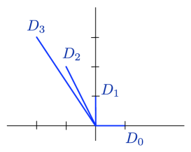
Figure 2: Toric fan for the $A_{2}$-fibration.

The regular representation is now $Q=\rho_{1}\oplus\rho_{2}\oplus\rho_{0}$ and the tensor product decomposition gives symmetric matrices

$$\big{(}a_{rs}^{(1)}\big{)}=\big{(}a_{rs}^{(2)}\big{)}=\left(\begin{matrix}1&1&1\\ 1&1&1\\ 1&1&1\end{matrix}\right)\ .$$ (7.4)

The associated quiver is

(7.5)

7.2 BPS partition functions

Let us start with the $U(1)$ gauge theory. The combinations $a_{rs}^{(1)}-a_{rs}^{(2)}$ vanish identically, and the boundary condition is imposed by choosing ${\boldsymbol{N}}=(1,0,\dots,0)$. Again the contribution (4.59) vanishes, as it should, while the second Chern character in the instanton action (4.7) has the same form as in (6.7) but with the sums now ranging over $0,1,\dots,n-1$. Let us evaluate this integral. It measures the triple intersection between two divisors, corresponding to two compact curves, with the divisor $\wp_{\infty}$ at infinity. The geometry we are considering is a trivial fibration of an $A_{n-1}$ singularity over an affine line. Therefore all the intersection numbers are essentially given by the intersections of curves in the exceptional locus of the blown up singularity in $\mathbb{C}^{2}$. However these intersections are still “fibred” over the affine line. For example, if two exceptional curves intersect at a point in the ALE geometry, then their intersection in the full Calabi–Yau threefold has the form ${\mathrm{pt}}\times{\mathbb{C}}$. In the full Calabi–Yau geometry the exceptional curves are actually non-compact divisors of the form ${\mathbb{P}}^{1}\times{\mathbb{C}}$. The intersection with the boundary divisor is only due to the non-compact factor ${\mathbb{C}}$.

We can therefore write the action as

$$\int_{\overline{X}}\,\omega\wedge{\rm ch}_{2}({\cal E})=-\sum_{m,r,s=0}^{n-1}\,\varphi_{m}\,\Big{(}a^{(2)}_{rs}-3\,\delta_{rs}\Big{)}\ k_{s}\,\frac{a}{|\Gamma|}\,\tilde{C}_{mr}\ ,$$ (7.6)

where the constant $a$ parametrizes the intersections with $\wp_{\infty}$ and

$$\tilde{C}=\left(\begin{matrix}0&0\\ 0&C^{-1}\end{matrix}\right)$$ (7.7)

with $C$ the intersection matrix (minus the $A_{n-1}$ Cartan matrix). The rest of the instanton action (4.63) reads as in (6.8). The integrals involved have the form

$$\Big{(}\,\int_{\overline{X}}\,c_{1}\big{(}{\cal O}_{\overline{X}}(1)\big{)}\wedge{\rm ch}_{2}({\cal R}_{r})\,\Big{)}_{r=0,1,\dots,n-1} = \frac{a}{|\Gamma|}\,(0,-2,-2,\dots,-2)\ ,$$

$$\Big{(}\,\int_{\overline{X}}\,c_{1}({\cal R}_{r})\wedge{\rm ch}_{2}\big{(}{\cal O}_{\overline{X}}(1)\big{)}\,\Big{)}_{r=0,1,\dots,n-1} = \frac{1}{2|\Gamma|}\,(0,b,b,\dots,b)\ ,$$ (7.8)

where we have parametrized the intersection indices of non-compact divisors of the form ${\mathrm{pt}}\times{\mathbb{C}}$ and ${\mathbb{P}}^{1}\times{\mathbb{C}}$ with the divisor at infinity by two integers $a$ and $b$ (whose precise values are not important at the moment).

To compute the instanton measure we consider the $\Gamma$-invariant part of the partial character

$${\cal T}^{+}_{\pi}=V_{\pi}-V_{\pi}\otimes V^{\vee}_{\pi}~{}\frac{(1-t_{1})\,(1-t_{2})}{t_{1}\,t_{2}}\ .$$ (7.9)

For the orbifold action (7.1) the terms proportional to $V_{\pi}\otimes V^{\vee}_{\pi}$ cancel pairwise upon substituting $t_{1}=\zeta$, $t_{2}=\zeta^{-1}$, and therefore

$$\big{(}{\cal T}^{+}_{\pi}\big{)}^{\Gamma}=|\pi_{0}|\ .$$ (7.10)

The instanton partition function for the rank one invariants is thus

$${\cal Z}_{{\mathbb{C}}^{2}/{\mathbb{Z}}_{n}\times\mathbb{C}}=\sum_{\pi}\,(-1)^{|\pi_{0}|}\ {\,\rm e}\,^{-S_{\mathrm{inst}}[\pi]}\ .$$ (7.11)

The orbifold group $\Gamma={\mathbb{Z}}_{n}$ has $n$ irreducible representations. Therefore it is natural to parametrize the partition function of orbifold invariants as

$$K^{\rm DT}_{{\mathbb{C}}^{2}/{\mathbb{Z}}_{n}\times\mathbb{C}}=\sum_{\pi}\,(-1)^{|\pi_{0}|}\ p_{0}^{|\pi_{0}|}\ p_{1}^{|\pi_{1}|}\ \cdots\ p_{n-1}^{|\pi_{n-1}|}\ ,$$ (7.12)

which precisely coincides with the result of [47]. This partition function can also be written in a product form [47]

$$K^{\rm DT}_{{\mathbb{C}}^{2}/{\mathbb{Z}}_{n}\times\mathbb{C}}=M(-p)^{n}\,\prod_{0<r\leq s<n}\,\widetilde{M}(p_{[r,s]},-p)\ ,$$ (7.13)

where $p=p_{0}\,p_{1}\cdots p_{n-1}$ and $p_{[r,s]}=p_{r}\,p_{r+1}\cdots p_{s}$. As before, the large radius partition function is that of closed topological string theory on the crepant resolution $X={\rm Hilb}^{\mathbb{Z}_{n}}(\mathbb{C}^{3})$ and can be computed with the topological vertex formalism [47, 86]; it can be obtained from the orbifold partition function (7.13) via the substitution $\widetilde{M}(p_{[r,s]},-p)\to M(p_{[r,s]},-p)$ of generalized MacMahon functions and suitable reparametrization. The partition function at the large radius point is connected to the reparametrized partition function at the orbifold point via the wall-crossing factor $M(-p)^{-n}\,K_{X}^{\rm top}(p,p_{1}^{-1},\dots,p_{n-1}^{-1})$ as in (1.1).

For example, let us again consider the particular case ${\mathbb{C}}^{2}/{\mathbb{Z}}_{3}\times\mathbb{C}$, where

$$K^{\rm DT}_{{\mathbb{C}}^{2}/{\mathbb{Z}}_{3}\times\mathbb{C}} = \sum_{\pi}\,(-1)^{|\pi_{0}|}\ p_{0}^{|\pi_{0}|}\ p_{1}^{|\pi_{1}|}\ p_{2}^{|\pi_{2}|}$$

$$= M(-p_{0}\,p_{1}\,p_{2})^{3}\,\widetilde{M}(p_{1},-p_{0}\,p_{1}\,p_{2})\,\widetilde{M}(p_{1}\,p_{2},-p_{0}\,p_{1}\,p_{2})\,\widetilde{M}(p_{2},-p_{0}\,p_{1}\,p_{2})\ .$$

The instanton action is given by

$$\int_{\overline{X}}\,\omega\wedge{\rm ch}_{2}({\cal E}) = \mbox{$\frac{a}{3}$}\,\big{(}\varphi_{1}\,(k_{0}-k_{1})+\varphi_{2}\,(k_{0}-k_{2})\big{)}\ ,$$

$$\int_{\overline{X}}\,\mathrm{ch}_{3}({\cal E}) = -\mbox{$\frac{a}{3}$}\,(-4k_{0}+2k_{1}+2k_{2})+\mbox{$\frac{1}{3}$}\,(k_{0}+k_{1}+k_{2})-\mbox{$\frac{b}{6}$}\,(-2k_{0}+k_{1}+k_{2})\ .$$ (7.15)

Identifying $k_{r}=|\pi_{r}|$ at the fixed points $\pi=\bigsqcup_{r}\,\pi_{r}$, we can write the instanton partition function (7.11) as

$${\cal Z}_{{\mathbb{C}}^{2}/{\mathbb{Z}}_{3}\times\mathbb{C}}=\sum_{\pi}\,(-1)^{|\pi_{0}|}\ q^{\frac{1}{6}\,((8a+2b+2)\,|\pi_{0}|-(4a+b-2)\,(|\pi_{1}|+|\pi_{2}|))}\ Q_{1}^{-\frac{a}{3}\,(|\pi_{0}|-|\pi_{1}|)}\ Q_{2}^{-\frac{a}{3}\,(|\pi_{0}|-|\pi_{2}|)}$$ (7.16)

where as before we have introduced the weighting variables $q={\,\rm e}\,^{-g_{s}}$ and $Q_{r}={\,\rm e}\,^{-\varphi_{r}}$ for $r=1,2$. The two partition functions (7.2) and (7.16) are related by the simple change of variables

$$p_{0} = q^{\frac{1}{6}\,(8a+2b+2)}\ Q_{1}^{-a/3}\ Q_{2}^{-a/3}\ ,$$

$$p_{1} = q^{-\frac{1}{6}\,(4a+b-2)}\ Q_{1}^{a/3}\ ,$$

$$p_{2} = q^{-\frac{1}{6}\,(4a+b-2)}\ Q_{2}^{a/3}\ ,$$ (7.17)

with $p=p_{0}\,p_{1}\,p_{2}=q$.

7.3 Coulomb branch invariants

Let us now turn to the non-abelian gauge theory. We consider the $U(N)$ gauge theory where the gauge symmetry is broken to $U(1)^{N}$ according to the pattern dictated by the framing vector ${\boldsymbol{N}}=(N_{0},N_{1},\dots,N_{n-1})$. From (LABEL:c1Naction)–(5.68) the instanton action now has the form

$$\int_{\overline{X}}\,\omega\wedge\omega\wedge c_{1}({\cal E}) = 0\ ,$$

$$\int_{\overline{X}}\,\omega\wedge{\rm ch}_{2}({\cal E}) = -\sum_{m,r,s=0}^{n-1}\,\varphi_{m}\Big{(}a^{(2)}_{rs}-3\,\delta_{rs}\Big{)}\ \sum_{l=1}^{N}\,|\pi_{l,s-b(l)}|\,\frac{a}{|\Gamma|}\,\tilde{C}_{mr}\ ,$$ (7.18)

$$\int_{\overline{X}}\,\mathrm{ch}_{3}({\cal E}) = -\sum_{r,s=0}^{n-1}\ \sum_{l=1}^{N}\,|\pi_{l,s-b(l)}|\,\bigg{(}\left(a_{rs}^{(2)}-3\delta_{rs}\right)\ \int_{\overline{X}}\,c_{1}\big{(}{\cal O}_{\overline{X}}(1)\big{)}\wedge{\rm ch}_{2}({\cal R}_{r})$$

$$\qquad\qquad\qquad+\,\left(a^{(2)}_{rs}-3\delta_{rs}\right)\ \int_{\overline{X}}\,c_{1}({\cal R}_{r})\wedge{\rm ch}_{2}\big{(}{\cal O}_{\overline{X}}(1)\big{)}\bigg{)}-\frac{\delta_{rs}}{|\Gamma|}\ ,$$

up to constant terms which are proportional to $N_{r}$ but independent of the instanton numbers; such terms can be safely ignored and absorbed into the normalization of the partition function. The integrals appearing here are given by (7.8).

Similarly we have to compute the instanton measure from (5.59). The second set of sums vanishes identically because of the choice of orbifold action (7.1), and we are left with

$${\cal K}(\vec{\pi};{\boldsymbol{N}})=\sum_{l=1}^{N}\ \sum_{r=0}^{n-1}\,|\pi_{l,r}|\ N_{r+b(l)}\ .$$ (7.20)

We can therefore write down the partition function for noncommutative Donaldson–Thomas invariants of type ${\boldsymbol{N}}$ in the concise form

$${\cal Z}_{{\mathbb{C}}^{2}/{\mathbb{Z}}_{n}\times\mathbb{C}}({\boldsymbol{N}}) = \sum_{\vec{\pi}}\,(-1)^{\sum_{l=1}^{N}\ \sum_{r=0}^{n-1}\,|\pi_{l,r}|\ N_{r+b(l)}}$$ (7.21)

$$\qquad\qquad\times\,q^{\int_{\overline{X}}\,{\rm ch}_{3}({\cal E}_{\vec{\pi}})}\ \prod_{m=1}^{n}\,Q_{m}^{\sum_{r,s=0}^{n-1}\,(a^{(2)}_{rs}-3\delta_{rs})\ \sum_{l=1}^{N}\,|\pi_{l,s-b(l)}|\,\frac{a}{|\Gamma|}\,\tilde{C}_{mr}}$$

where $Q_{m}={\,\rm e}\,^{-\varphi_{m}}$.

To clarify the content of this formula, let us return to our particular example ${\mathbb{C}}^{2}/{\mathbb{Z}}_{3}\times\mathbb{C}$. For concreteness, let us choose the rank $N=5$ with the boundary condition ${\boldsymbol{N}}=(2,2,1)$. For the boundary function $b(l)$, which to an index $l=1,\dots,N$ associates the index of the irreducible representation associated with the Higgs field vacuum expectation value $e_{l}$, this implies the assignments

$$b(1) = 0\ \Longrightarrow\ e_{1}\longleftrightarrow\rho_{0}\ ,$$

$$b(2) = 0\ \Longrightarrow\ e_{2}\longleftrightarrow\rho_{0}\ ,$$

$$b(3) = 1\ \Longrightarrow\ e_{3}\longleftrightarrow\rho_{1}\ ,$$

$$b(4) = 1\ \Longrightarrow\ e_{4}\longleftrightarrow\rho_{1}\ ,$$

$$b(5) = 2\ \Longrightarrow\ e_{5}\longleftrightarrow\rho_{2}\ .$$ (7.22)

Since in this case one has

$$\sum_{l=1}^{5}\,|\pi_{l,0-b(l)}| = |\pi_{1,0}|+|\pi_{2,0}|+|\pi_{3,2}|+|\pi_{4,2}|+|\pi_{5,1}|\ ,$$

$$\sum_{l=1}^{5}\,|\pi_{l,1-b(l)}| = |\pi_{1,1}|+|\pi_{2,1}|+|\pi_{3,0}|+|\pi_{4,0}|+|\pi_{5,2}|\ ,$$

$$\sum_{l=1}^{5}\,|\pi_{l,2-b(l)}| = |\pi_{1,2}|+|\pi_{2,2}|+|\pi_{3,1}|+|\pi_{4,1}|+|\pi_{5,0}|\ ,$$ (7.23)

the instanton action can be written as (again up to irrelevant constant terms)

$$\int_{\overline{X}}\,\omega\wedge{\rm ch}_{2}({\cal E}_{\vec{\pi}}) = \frac{a}{3}\,\Big{(}\varphi_{1}\,\big{(}|\pi_{1,0}|-|\pi_{1,1}|+|\pi_{2,0}|-|\pi_{2,1}|+|\pi_{3,2}|-|\pi_{3,0}|$$ (7.25)

$$\qquad\qquad+\,|\pi_{4,2}|-|\pi_{4,0}|+|\pi_{5,1}|-|\pi_{5,2}|\big{)}$$

$$\qquad+\,\varphi_{2}\,\big{(}|\pi_{1,0}|-|\pi_{1,2}|+|\pi_{2,0}|-|\pi_{2,2}|+|\pi_{3,2}|-|\pi_{3,1}|$$

$$\qquad\qquad\qquad+\,|\pi_{4,2}|-|\pi_{4,1}|+|\pi_{5,1}|-|\pi_{5,0}|\big{)}\Big{)}$$

and

$$\int_{\overline{X}}\,\mathrm{ch}_{3}({\cal E}_{\vec{\pi}}) = \frac{1}{6}\,\Big{(}(8a+2b+2)\,\big{(}|\pi_{1,0}|+|\pi_{2,0}|+|\pi_{3,2}|+|\pi_{4,2}|+|\pi_{5,1}|\big{)}$$ (7.28)

$$\qquad-\,(4a+b-2)\,\big{(}|\pi_{1,1}|+|\pi_{1,2}|+|\pi_{2,1}|+|\pi_{2,2}|+|\pi_{3,0}|+|\pi_{3,1}|$$

$$\qquad\qquad\qquad\qquad\qquad+\,|\pi_{4,0}|+|\pi_{4,1}|+|\pi_{5,2}|+|\pi_{5,0}|\big{)}\Big{)}\ .$$

Similarly the instanton measure (7.20) in this case becomes

$${\cal K}\big{(}\vec{\pi}\,;\,{\boldsymbol{N}}=(2,2,1)\big{)}=|\pi_{1,2}|+|\pi_{2,2}|+|\pi_{3,1}|+|\pi_{4,1}|+|\pi_{5,0}|\ ,$$ (7.29)

where we have dropped the even parity terms which do not affect the alternating sign of the fluctuation determinant. By using the change of variables (7.17) of the $U(1)$ gauge theory we can write the partition function as

$${\cal Z}_{{\mathbb{C}}^{2}/{\mathbb{Z}}_{3}\times\mathbb{C}}\big{(}{\boldsymbol{N}}=(2,2,1)\big{)} = \sum_{\pi_{1}}\,(-1)^{|\pi_{1,2}|}\,p_{0}^{|\pi_{1,0}|}\,p_{1}^{|\pi_{1,1}|}\,p_{2}^{|\pi_{1,2}|}\ \sum_{\pi_{2}}\,(-1)^{|\pi_{2,2}|}\,p_{0}^{|\pi_{2,0}|}\,p_{1}^{|\pi_{2,1}|}\,p_{2}^{|\pi_{2,2}|}$$ (7.32)

$$\times\ \sum_{\pi_{3}}\,(-1)^{|\pi_{3,1}|}\,p_{0}^{|\pi_{3,2}|}\,p_{1}^{|\pi_{3,0}|}\,p_{2}^{|\pi_{3,1}|}\ \sum_{\pi_{4}}\,(-1)^{|\pi_{4,1}|}\,p_{0}^{|\pi_{4,2}|}\,p_{1}^{|\pi_{4,0}|}\,p_{2}^{|\pi_{4,1}|}$$

$$\times\ \sum_{\pi_{5}}\,(-1)^{|\pi_{5,0}|}\,p_{0}^{|\pi_{5,1}|}\,p_{1}^{|\pi_{5,2}|}\,p_{2}^{|\pi_{5,0}|}\ .$$

By repeatedly applying (7.2) this partition function can be expressed in closed form as a product of generalized MacMahon functions. For example the sum

$$\sum_{\pi_{3}}\,(-1)^{|\pi_{3,1}|}\,p_{0}^{|\pi_{3,2}|}\,p_{1}^{|\pi_{3,0}|}\,p_{2}^{|\pi_{3,1}|}=\sum_{\pi_{3}}\,(-1)^{|\pi_{3,0}|}\,p_{0}^{|\pi_{3,2}|}\,(-p_{1})^{|\pi_{3,0}|}\,(-p_{2})^{|\pi_{3,1}|}$$ (7.33)

is equal to (7.2) upon redefining $p_{0}\rightarrow p_{2}$, $p_{1}\rightarrow-p_{0}$ and $p_{2}\rightarrow-p_{1}$. One then finds

$${\cal Z}_{{\mathbb{C}}^{2}/{\mathbb{Z}}_{3}\times\mathbb{C}}\big{(}{\boldsymbol{N}}=(2,2,1)\big{)} = M(-q)^{15}\,\widetilde{M}(p_{0},-q)^{3}\,\widetilde{M}(p_{1},-q)^{3}\,\widetilde{M}(-p_{2},-q)^{4}$$ (7.35)

$$\times\,\widetilde{M}(p_{0}\,p_{1},-q)\,\widetilde{M}(-p_{1}\,p_{2},-q)^{2}\,\widetilde{M}(-p_{0}\,p_{2},-q)^{2}\ .$$

By expanding these functions one obtains expressions for the noncommutative Donaldson–Thomas invariants ${\tt NC}_{0}({\boldsymbol{k}},{\boldsymbol{N}})$ of type ${\boldsymbol{N}}=(2,2,1)$ for the orbifold geometry ${\mathbb{C}}^{2}/{\mathbb{Z}}_{3}\times\mathbb{C}$. These invariants, although numerically different from those of the $U(1)$ gauge theory, can also be derived from rank one quiver generalized Donaldson–Thomas invariants via the formula (5.42). By taking the logarithm of the partition function (7.35) we obtain the free energy

$${\cal F}_{{\mathbb{C}}^{2}/{\mathbb{Z}}_{3}\times\mathbb{C}}\big{(}{\boldsymbol{N}}=(2,2,1)\big{)} = \sum_{n,l=1}^{\infty}\,(-1)^{n\,l}\,\frac{n}{l}\,\Big{(}15\,p_{0}^{n\,l}\,p_{1}^{n\,l}\,p_{2}^{n\,l}+3\,p_{0}^{n\,l}\,p_{1}^{(n+1)\,l}\,p_{2}^{n\,l}+3\,p_{0}^{n\,l}\,p_{1}^{(n-1)\,l}\,p_{2}^{n\,l}$$

$$\qquad+\,2(-1)^{l}\,p_{0}^{n\,l}\,p_{1}^{(n+1)\,l}\,p_{2}^{(n+1)\,l}+2(-1)^{l}\,p_{0}^{n\,l}\,p_{1}^{(n-1)\,l}\,p_{2}^{(n-1)\,l}$$

$$\qquad+\,4(-1)^{l}\,p_{0}^{n\,l}\,p_{1}^{n\,l}\,p_{2}^{(n+1)\,l}+4(-1)^{l}\,p_{0}^{n\,l}\,p_{1}^{n\,l}\,p_{2}^{(n-1)\,l}$$

$$\qquad+\,2(-1)^{l}\,p_{0}^{(n+1)\,l}\,p_{1}^{n\,l}\,p_{2}^{(n+1)\,l}+2(-1)^{l}\,p_{0}^{(n-1)\,l}\,p_{1}^{n\,l}\,p_{2}^{(n-1)\,l}$$

$$\qquad+\,3\,p_{0}^{(n+1)\,l}\,p_{1}^{n\,l}\,p_{2}^{n\,l}+3\,p_{0}^{(n-1)\,l}\,p_{1}^{n\,l}\,p_{2}^{n\,l}$$

$$\qquad+\,p_{0}^{(n+1)\,l}\,p_{1}^{(n+1)\,l}\,p_{2}^{n\,l}+p_{0}^{(n-1)\,l}\,p_{1}^{(n-1)\,l}\,p_{2}^{n\,l}\Big{)}\ .$$

By combining terms one finds that this expression indeed fits the pattern of (5.42). For example

$$\sum_{n,l=1}^{\infty}\,(-1)^{n\,l}\,3\,\frac{n}{l}\,p_{0}^{n\,l}\,p_{1}^{(n-1)\,l}\,p_{2}^{n\,l}+\sum_{n,l=1}^{\infty}\,(-1)^{n\,l+l}\,2\,\frac{n}{l}\,p_{0}^{(n+1)\,l}\,p_{1}^{n\,l}\,p_{2}^{(n+1)\,l}$$ (7.38)

$$\qquad\qquad\ =\ \sum_{n,l=1}^{\infty}\,(-1)^{n\,l}\,\frac{3n+2n-2}{l}\,p_{0}^{n\,l}\,p_{1}^{(n-1)\,l}\,p_{2}^{n\,l}$$ (7.39)

$$\qquad\qquad\ =\ \sum_{n,l=1}^{\infty}\,(-1)^{2n\,l+2(n-1)\,l+n\,l}\ \big{(}2n\,l+2(n-1)\,l+n\,l\big{)}\ \left(\frac{1}{l^{2}}\right)\,p_{0}^{n\,l}\,p_{1}^{(n-1)\,l}\,p_{2}^{n\,l}\ ,$$

which implies

$$\overline{{\tt DT}}_{0}({\boldsymbol{k}})=-\frac{1}{l^{2}}\qquad\text{for}\quad{\boldsymbol{k}}=(n\,l,n\,l-l,n\,l)\qquad\text{with}\quad n,l\geq 1\ .$$ (7.40)

Proceeding in a similar way for the remaining terms, we obtain the non-vanishing rank one quiver invariants

$$\overline{{\tt DT}}_{0}({\boldsymbol{k}})=-\frac{1}{l^{2}}\qquad\text{for}\quad{\boldsymbol{k}}=\left\{\begin{matrix}(n\,l,n\,l+l,n\,l)\ ,\quad n\geq 0\ ,\ l\geq 1\ ,\\ (n\,l-l,n\,l,n\,l)\ ,\quad n,l\geq 1\ ,\\ (n\,l+l,n\,l,n\,l)\ ,\quad n\geq 0\ ,\ l\geq 1\ ,\\ (n\,l-l,n\,l-l,n\,l)\ ,\quad n,l\geq 1\ ,\\ (n\,l+l,n\,l+l,n\,l)\ ,\quad n\geq 0\ ,\ l\geq 1\ ,\end{matrix}\right.$$ (7.41)

and

$$\overline{{\tt DT}}_{0}\big{(}{\boldsymbol{k}}=(k,k,k)\big{)}=-3\,\sum_{l\geq 1\,:\,l|k}\,\frac{1}{l^{2}}\qquad\mbox{for}\quad k\geq 1\ .$$ (7.42)

Comparing with (5.39) we obtain the non-vanishing integer BPS invariants

$$\widehat{{\tt DT}}_{0}({\boldsymbol{k}})=-1\qquad\text{for}\quad{\boldsymbol{k}}=\left\{\begin{matrix}(n,n-1,n)\ ,\quad n\geq 1\ ,\\ (n,n+1,n)\ ,\quad n\geq 0\ ,\\ (n-1,n,n)\ ,\quad n\geq 1\ ,\\ (n+1,n,n)\ ,\quad n\geq 0\ ,\\ (n-1,n-1,n)\ ,\quad n\geq 1\ ,\\ (n+1,n+1,n)\ ,\quad n\geq 0\ ,\end{matrix}\right.$$ (7.43)

and

$$\widehat{{\tt DT}}_{0}\big{(}{\boldsymbol{k}}=(k,k,k)\big{)}=-3\qquad\mbox{for}\quad k\geq 1\ .$$ (7.44)

These invariants agree with those obtained in [18] from the rank one partition function (7.2).

We can similarly generalize our arguments to get a compact solution for the noncommutative Donaldson–Thomas invariants for any $A$-fibred threefold of the form ${\mathbb{C}}^{2}/{\mathbb{Z}}_{n}\times\mathbb{C}$ and any boundary condition fixed by a framing vector ${\boldsymbol{N}}$. The partition function then assumes the form

$${\cal Z}_{{\mathbb{C}}^{2}/{\mathbb{Z}}_{n}\times\mathbb{C}}({\boldsymbol{N}})=\sum_{\vec{\pi}}\,(-1)^{\sum_{l=1}^{N}\ \sum_{r=0}^{n-1}\,|\pi_{l,r}|\ N_{r+b(l)}}\ p_{0}^{\sum_{l=1}^{N}\,|\pi_{l,0-b(l)}|}\ \cdots\ p_{n-1}^{\sum_{l=1}^{N}\,|\pi_{l,n-1-b(l)}|}\ .$$ (7.45)

As we did above, for a given fixed framing vector ${\boldsymbol{N}}$ it is possible to express this formula in a closed form as a product of MacMahon functions $M(q)$ and $\widetilde{M}(x,q)$. The corresponding quiver invariants, independent of $N$ and ${\boldsymbol{N}}$, can again be computed explicitly from the formulas (5.42) and (5.39). The integer BPS invariants in this case are computed in [18, Section 7.5.4] from the rank one partition function (7.13).

7.4 Higher rank wall-crossing formulas

We will now describe the wall-crossing formula for Coulomb branch invariants. Although the wall contributions are all contained in the quiver BPS invariants $\widehat{{\tt DT}}_{\mu}({\boldsymbol{k}})$, which are unchanged by wall-crossing in this case [18], it is interesting to examine if the noncommutative invariants ${\tt NC}_{\mu}({\boldsymbol{k}},{\boldsymbol{N}})$ have wall-crossings of their own. Here we consider only very particular walls of stability. In general, there will be walls corresponding to separated D6 branes colliding and forming a bound state; these walls are not included in our analysis below, and to get them one should use a non-primitive wall-crossing formula. On the other hand, since the D6 branes are well-separated in the Coulomb branch, it is reasonable to expect that the walls affecting D2–D0 bound states are reached before the walls corresponding to D6 bound states.

The large radius partition function for Coulomb branch invariants can be computed from the $U(N)$ instanton contributions to the noncommutative gauge theory on the ALE resolution $X$ of the $A_{n-1}$-fibration [37]. It is given by a simple modification of the partition function for topological string theory on $X$ as

$$K_{X}^{\rm DT}(q,p_{1},\dots,p_{n-1};N)=M\big{(}(-1)^{N}\,q\big{)}^{n\,N}\,\prod_{0<r\leq s<n}\,M\big{(}p_{[r,s]}\,,\,(-1)^{N}\,q\big{)}^{N}\ .$$ (7.46)

From the wall-crossing formula in the rank one case and the explicit expression (7.45), it follows that this function is related to the partition function for Coulomb branch invariants in the case that the asymptotic Higgs fields $e_{l}$ all transform in the trivial representation $\rho_{0}$ of the orbifold group $\Gamma=\mathbb{Z}_{n}$, i.e. $b(l)=0$ for all $l=1,\dots,N$, or equivalently $N_{0}=N$ while $N_{r}=0$ for all $r=1,\dots,n-1$. One then finds the non-abelian wall-crossing formula

$${\cal Z}_{{\mathbb{C}}^{2}/{\mathbb{Z}}_{n}\times\mathbb{C}}\big{(}q,p_{1},\dots,p_{n-1}\,;\,{\boldsymbol{N}}=(N,0,\dots,0)\big{)}$$ (7.47)

$$\qquad\qquad\ =\ M\big{(}(-1)^{N}\,q\big{)}^{-n\,N}\,K_{X}^{\rm DT}(q,p_{1},\dots,p_{n-1};N)\,K_{X}^{\rm DT}(q,p_{1}^{-1},\dots,p^{-1}_{n-1};N)\ .$$

The wall-crossing factor $M\big{(}(-1)^{N}\,q\big{)}^{-n\,N}\,K_{X}^{\rm DT}(q,p_{1}^{-1},\dots,p^{-1}_{n-1};N)$ in (7.47) describes the crossing of an infinite number of walls of marginal stability, separating different chambers in the Kähler moduli space, in going from the orbifold point to the large radius point. To identify the individual walls, let us first recall the situation in the $U(1)$ gauge theory as studied in [85] (see also [87]). In this context the walls are determined by the affine Lie algebra structure associated with the McKay quiver. If we denote by ${\boldsymbol{\theta}}$ a $\theta$-stability parameter for the (unframed) quiver, then the walls of marginal stability are determined by

$${\cal W}_{\hat{{\boldsymbol{k}}}}=\big{\{}{\boldsymbol{\theta}}\in{\mathbb{R}}^{n}\ \big{|}\ {\boldsymbol{\theta}}\cdot\hat{{\boldsymbol{k}}}=0\ ,\ \hat{{\boldsymbol{k}}}\in\hat{\Delta}^{+}\big{\}}$$ (7.48)

where $\hat{\Delta}^{+}$ is the set of affine positive roots. These walls connect different chambers. Of particular relevance among them is the wall determined by the imaginary root $\hat{{\boldsymbol{k}}}{}^{\rm im}$ of the affine $A_{n-1}$ Lie algebra, which corresponds to the regular representation of $\Gamma=\mathbb{Z}_{n}$ and separates the Donaldson–Thomas chamber from the Pandharipande–Thomas chamber. Our wall-crossing formulas do not include this wall.

Fix a real positive root ${\boldsymbol{k}}$ and consider stability parameters on both sides of the associated wall, ${\boldsymbol{\theta}}_{{\boldsymbol{k}}}^{+}$ and ${\boldsymbol{\theta}}_{{\boldsymbol{k}}}^{-}$. Then our vector space $V$ can be identified with the unique ${\boldsymbol{\theta}}_{{\boldsymbol{k}}}$-stable module over the path algebra of dimension vector ${\boldsymbol{k}}$ constructed in [85]. Therefore the wall-crossing formula of [85, Theorem 4.15] is given by

$${\cal Z}_{{\mathbb{C}}^{2}/{\mathbb{Z}}_{n}\times\mathbb{C}}^{{\boldsymbol{\theta}}_{{\boldsymbol{k}}}^{-}}({\boldsymbol{p}})=\big{(}1-(-1)^{k_{0}}\,{\boldsymbol{p}}^{{\boldsymbol{k}}}\big{)}^{-k_{0}}\,{\cal Z}_{{\mathbb{C}}^{2}/{\mathbb{Z}}_{n}\times\mathbb{C}}^{{\boldsymbol{\theta}}_{{\boldsymbol{k}}}^{+}}({\boldsymbol{p}})\ ,$$ (7.49)

where the instanton charge $k_{0}=|\pi_{0}|$ is singled out by the framing condition. It follows from (7.47) that the proof of [85, Theorem 4.15] can be adapted to our more general situation to give

$${\cal Z}_{{\mathbb{C}}^{2}/{\mathbb{Z}}_{n}\times\mathbb{C}}^{{\boldsymbol{\theta}}_{{\boldsymbol{k}}}^{-}}\big{(}{\boldsymbol{p}}\,;\,{\boldsymbol{N}}=(N,0,\dots,0)\big{)}=\big{(}1-(-1)^{k_{0}\,N}\,{\boldsymbol{p}}^{{\boldsymbol{k}}}\big{)}^{-k_{0}\,N}\,{\cal Z}_{{\mathbb{C}}^{2}/{\mathbb{Z}}_{n}\times\mathbb{C}}^{{\boldsymbol{\theta}}_{{\boldsymbol{k}}}^{+}}\big{(}{\boldsymbol{p}}\,;\,{\boldsymbol{N}}=(N,0,\dots,0)\big{)}\ ,$$ (7.50)

which establishes the wall-crossing formula for noncommutative Donaldson–Thomas invariants of type ${\boldsymbol{N}}=(N,0,\dots,0)$.

This formula is just a mild generalization of the Kontsevich–Soibelman wall-crossing formula. In this case the invariants all jump together; in each $U(1)$ sector the wall-crossing formula is the same up to a redefinition of the assignments of parameters to irreducible representations and some signs. Thus each $U(1)$ factor jumps separately while the walls are the same for every sector. We do not know how to extend these considerations to generic framing vectors ${\boldsymbol{N}}$ corresponding to more general boundary conditions on the Higgs fields.

8 An example with compact four cycles:  ${\mathbb{C}}^{3}/{\mathbb{Z}}_{3}$

8.1 Geometry and representation theory

Our next example is the ${\mathbb{C}}^{3}/{\mathbb{Z}}_{3}$ orbifold with weights $r_{1}=r_{2}=r_{3}=1$ that was studied in Section 3.2 and Section 5.3; its unique Calabi–Yau crepant resolution given by the ${\mathbb{Z}}_{3}$-Hilbert scheme $X=\mathrm{Hilb}^{{\mathbb{Z}}_{3}}({\mathbb{C}}^{3})$ is the total space of the fibration ${\cal O}_{{\mathbb{P}}^{2}}(-3)\rightarrow{\mathbb{P}}^{2}$, also known as the local del Pezzo surface of degree zero. This geometry has one compact divisor, the base $E\cong{\mathbb{P}}^{2}$ of the fibration, and three rational curves which are homologous. Its fan $\Sigma\subset\mathbb{Z}^{3}$ is generated by the vectors

$$D_{1}=(-1,1,1)\ ,\qquad D_{2}=(1,0,1)\qquad\mbox{and}\qquad D_{3}=(0,1,1)\ ,$$ (8.1)

and the toric diagram for the resolved geometry is depicted in Figure 3.

Figure 3: Toric fan for the local del Pezzo surface of degree zero.

The linear equivalences between the divisors are given by

$$D_{\alpha}\sim D_{\beta}\qquad\mbox{and}\qquad 3D_{\alpha}+E\sim 0\qquad\mbox{for}\quad\alpha,\beta=1,2,3\ .$$ (8.2)

The Mori cone has a single generator

$$C=D_{1}\cdot E=D_{2}\cdot E=D_{3}\cdot E$$ (8.3)

dual to the generator of the Kähler cone which is given by any of the linearly equivalent non-compact divisors $D_{\alpha}$. In particular $E\cdot E\cdot E=9$.

The basis of tautological bundles is indexed by the irreducible representations $\rho_{r}$ with $r=0,1,2$. The defining representation, which describes the action (3.21) of ${\mathbb{Z}}_{3}$ on the coordinates of ${\mathbb{C}}^{3}$, is $Q=\rho_{1}\oplus\rho_{1}\oplus\rho_{1}$. The tensor product decompositions (4.16) for $i=1,2$ yield the matrices

$$\big{(}a_{rs}^{(1)}\big{)}=\left(\begin{matrix}0&0&3\\ 3&0&0\\ 0&3&0\end{matrix}\right)\qquad\mbox{and}\qquad\big{(}a_{rs}^{(2)}\big{)}=\left(\begin{matrix}0&3&0\\ 0&0&3\\ 3&0&0\end{matrix}\right)$$ (8.4)

with $a_{rs}^{(2)}=a_{sr}^{(1)}$. The associated quiver is given in (5.6).

If we write the original coordinates of ${\mathbb{C}}^{3}$ as $(z_{1},z_{2},z_{3})$, then the rational curves are locally described by invariant ratios of monomials of the form $z_{1}/z_{2}$ and cyclic permutations thereof. Therefore they correspond to the character $\rho_{1}$, and a generator of $H^{2}(X,{\mathbb{Z}})$ dual to the curve class $C$ is given by $c_{1}({\cal R}_{1})$. In the fan $\Sigma$ there are now three toric curves intersecting in a vertex of valence $3$ and therefore, following the decoration procedure described in Section 4.6, we associate the character $\rho_{2}=\rho_{1}\otimes\rho_{1}$ to the vertex. This gives one relation in the Picard group $\mathrm{Pic}(X)$, namely ${\cal R}_{2}={\cal R}_{1}\otimes{\cal R}_{1}$. In particular the second Chern class of ${\cal V}=\left({\cal R}_{1}\oplus{\cal R}_{1}\right)\ominus\left({\cal R}_{2}\oplus{\cal O}_{X}\right)$ generates $H^{4}(X,{\mathbb{Z}})$ and is dual to the exceptional divisor with

$$\int_{{\mathbb{P}}^{2}}\,c_{2}({\cal V})=1\ .$$ (8.5)

In this case we have $c_{1}({\cal R}_{2})=2c_{1}({\cal R}_{1})$ and $c_{2}({\cal V})=c_{1}({\cal R}_{1})\wedge c_{1}({\cal R}_{1})$, with ${\cal R}_{\alpha}={\cal O}_{X}(\alpha\,D)$ where $D$ is one of the linearly equivalent divisors $D_{\alpha}$ which is dual to the class $c_{1}({\cal R}_{1})$ corresponding to ${\mathbb{P}}^{2}$.

8.2 BPS partition functions

We begin again with the $U(1)$ gauge theory. As explained in Section 4.5 we need only consider the boundary condition given by the framing vector ${\boldsymbol{N}}=(1,0,0)$. In the present geometry we can also consider a term involving the first Chern class, which measures the D4 brane charge. Firstly, having determined both a basis of $H^{4}(X,{\mathbb{Z}})$ and $H^{2}(X,{\mathbb{Z}})$ we can write

$$\omega=\varphi\ c_{1}({\cal R}_{1})\qquad\mbox{and}\qquad\omega\wedge\omega=\varsigma\ c_{2}({\cal V})=\varsigma\ c_{1}({\cal R}_{1})\wedge c_{1}({\cal R}_{1})\ .$$ (8.6)

From the general form of the instanton action (4.59) we have

$$\int_{\overline{X}}\,\omega\wedge\omega\wedge c_{1}({\cal E}) = -\varsigma\,\sum_{r,s=0}^{2}\,\left(a^{(1)}_{rs}-a^{(2)}_{rs}\right)\,k_{s}\,\int_{\overline{X}}\,c_{2}({\cal V})\wedge c_{1}({\cal R}_{r})$$ (8.7)

$$= \varsigma\,\left(3k_{0}-6k_{1}+3k_{2}\right)\,\int_{\overline{X}}\,c_{1}({\cal R}_{1})\wedge c_{1}({\cal R}_{1})\wedge c_{1}({\cal R}_{1})\ .$$

On the other hand since $E\cdot E\cdot E=9$ and $E\sim-3D$, we see that

$$\int_{\overline{X}}\,c_{1}({\cal R}_{1})\wedge c_{1}({\cal R}_{1})\wedge c_{1}({\cal R}_{1})=D\cdot D\cdot D=-\frac{1}{3}\ .$$ (8.8)

Similarly, from (4.7) one has

$$\int_{\overline{X}}\,\omega\wedge{\rm ch}_{2}({\cal E}) = -\varphi\,\sum_{r,s=0}^{2}\,\bigg{(}\left(a^{(1)}_{rs}-a^{(2)}_{rs}\right)\ k_{s}\ \int_{\overline{X}}\,c_{1}({\cal R}_{1})\wedge{\rm ch}_{2}({\cal R}_{r})$$

$$\qquad\qquad\qquad+\,\left(a^{(2)}_{rs}-3\,\delta_{rs}\right)\ k_{s}\,\int_{\overline{X}}\,c_{1}({\cal R}_{1})\wedge c_{1}({\cal R}_{r})\ c_{1}\big{(}{\cal O}_{\overline{X}}(1)\big{)}\bigg{)}$$

$$= -\mbox{$\frac{1}{6}$}\,\varphi\,\left(9k_{0}-12k_{1}+3k_{2}\right)$$ (8.11)

$$-\,\varphi\,\left(6k_{0}-3k_{1}-3k_{2}\right)\,\int_{\overline{X}}\,c_{1}({\cal R}_{1})\wedge c_{1}({\cal R}_{1})\wedge c_{1}\big{(}{\cal O}_{\overline{X}}(1)\big{)}\ .$$

The last term of the instanton action (4.63) reads

$$\int_{\overline{X}}\,{\rm ch}_{3}({\cal E}) = -\sum_{r,s=0}^{2}\,\bigg{(}\left(a^{(1)}_{rs}-a^{(2)}_{rs}\right)\,k_{s}\,\int_{\overline{X}}\,{\rm ch}_{3}({\cal R}_{r})-\left(a^{(2)}_{rs}-3\delta_{rs}\right)\,k_{s}\,\int_{\overline{X}}\,c_{1}({\cal R}_{r})\wedge{\rm ch}_{2}\big{(}{\cal O}_{\overline{X}}(1)\big{)}$$ (8.13)

$$\qquad\qquad+\,\left(a^{(2)}_{rs}-3\delta_{rs}\right)\ k_{s}\ \int_{\overline{X}}\,{\rm ch}_{2}({\cal R}_{r})\wedge c_{1}\big{(}{\cal O}_{\overline{X}}(1)\big{)}-\delta_{rs}\,\frac{k_{s}}{3}\bigg{)}$$

$$= -\mbox{$\frac{1}{6}$}\,\left(7k_{0}-8k_{1}+k_{2}\right)+\mbox{$\frac{1}{2}$}\,\left(6k_{0}-3k_{1}-3k_{2}\right)\ \int_{\overline{X}}\,c_{1}({\cal R}_{1})\wedge c_{1}\big{(}{\cal O}_{\overline{X}}(1)\big{)}\wedge c_{1}\big{(}{\cal O}_{\overline{X}}(1)\big{)}$$

$$-\,\mbox{$\frac{1}{2}$}\,\left(12k_{0}-3k_{1}-9k_{2}\right)\ \int_{\overline{X}}\,c_{1}({\cal R}_{1})\wedge c_{1}({\cal R}_{1})\wedge c_{1}\big{(}{\cal O}_{\overline{X}}(1)\big{)}+\mbox{$\frac{1}{3}$}\,\left(k_{0}+k_{1}+k_{2}\right)\ .$$

To evaluate the intersection indices arising here we work as follows. This geometry contains a compact divisor. By using linear equivalence, it is possible to rephrase the analysis of Section 7.2 in such a way that only compact cycles enter, the divisor and rational curves. Therefore all the integrals involving $c_{1}({\cal O}_{\overline{X}}(1))$ and $c_{1}({\cal R}_{1})$ compute the intersection indices between elements of the exceptional locus with the divisor at infinity. We assume that the compactification divisor $\wp_{\infty}$ is chosen so that these intersections vanish. Under this assumption, the instanton action finally becomes

$$\int_{\overline{X}}\,{\rm ch}_{3}({\cal E}) = -\mbox{$\frac{1}{6}$}\,\left(5k_{0}-10k_{1}-k_{2}\right)\ ,$$

$$\int_{\overline{X}}\,\omega\wedge{\rm ch}_{2}({\cal E}) = -\mbox{$\frac{1}{2}$}\,\varphi\,\left(3k_{0}-4k_{1}+k_{2}\right)\ ,$$

$$\int_{\overline{X}}\,\omega\wedge\omega\wedge c_{1}({\cal E}) = -\varsigma\,\left(k_{0}-2k_{1}+k_{2}\right)\ .$$ (8.15)

We compute the instanton measure by taking the ${\mathbb{Z}}_{3}$-invariant part of the character (5.24). For this, let us decompose $V_{\pi}=\textsf{V}_{0}\oplus\textsf{V}_{1}\oplus\textsf{V}_{2}$ at a fixed point $\pi$ according to the ${\mathbb{Z}}_{3}$-action as before, where now each term is of order three. The explicit form of the partial character (7.9) is now

$$\mathcal{T}_{\pi}^{+} = (\textsf{V}_{0}\oplus\textsf{V}_{1}\oplus\textsf{V}_{2})$$

$$-\,\Big{(}\,\frac{1}{t_{1}\,t_{2}}-\frac{1}{t_{2}}-\frac{1}{t_{1}}+1\,\Big{)}\,\big{(}\textsf{V}_{0}\otimes\textsf{V}^{\vee}_{0}\ \oplus\ \textsf{V}_{0}\otimes\textsf{V}^{\vee}_{1}\ \oplus\ \textsf{V}_{0}\otimes\textsf{V}^{\vee}_{2}\ \oplus\ \textsf{V}_{1}\otimes\textsf{V}^{\vee}_{0}$$

$$\qquad\qquad\qquad\qquad\oplus\ \textsf{V}_{1}\otimes\textsf{V}^{\vee}_{1}\ \oplus\ \textsf{V}_{1}\otimes\textsf{V}^{\vee}_{2}\ \oplus\ \textsf{V}_{2}\otimes\textsf{V}^{\vee}_{0}\ \oplus\ \textsf{V}_{2}\otimes\textsf{V}^{\vee}_{1}\ \oplus\ \textsf{V}_{2}\otimes\textsf{V}^{\vee}_{2}\big{)}\ .$$

It is easy to find the invariant part by substituting $t_{\alpha}=\zeta$ to get the virtual dimension (modulo $2$)

$$\big{(}\mathcal{T}_{\pi}^{+}\big{)}^{{\mathbb{Z}}_{3}} = {\rm vdim}_{\mathbb{C}}\big{(}\textsf{V}_{0}-(\textsf{V}_{0}\otimes\textsf{V}^{\vee}_{0}\ \oplus\ \textsf{V}_{1}\otimes\textsf{V}^{\vee}_{1}\ \oplus\ \textsf{V}_{2}\otimes\textsf{V}^{\vee}_{2})$$ (8.17)

$$+\,2(\textsf{V}_{0}\otimes\textsf{V}^{\vee}_{2}\ \oplus\ \textsf{V}_{1}\otimes\textsf{V}^{\vee}_{0}\ \oplus\ \textsf{V}_{2}\otimes\textsf{V}^{\vee}_{1})-(\textsf{V}_{0}\otimes\textsf{V}^{\vee}_{1}\ \oplus\ \textsf{V}_{1}\otimes\textsf{V}^{\vee}_{2}\ \oplus\ \textsf{V}_{2}\otimes\textsf{V}^{\vee}_{0})\big{)}$$

$$= |\pi_{1}|+|\pi_{2}|+|\pi_{0}|\,|\pi_{1}|+|\pi_{0}|\,|\pi_{2}|+|\pi_{1}|\,|\pi_{2}|\ ,$$

where we recall that the fixed points are classified by coloured partitions $\pi=\pi_{0}\sqcup\pi_{1}\sqcup\pi_{2}$. This result agrees with that quoted in [47, Remark A.5], and it shows that the equivariant Euler characteristic of the obstruction bundle on the quiver variety at a fixed point $\pi$ is given by

$$\chi_{{\mathbb{T}}^{3}}(\mathcal{N}_{\pi})=(-1)^{|\pi_{1}|+|\pi_{2}|+|\pi_{0}|\,|\pi_{1}|+|\pi_{0}|\,|\pi_{2}|+|\pi_{1}|\,|\pi_{2}|}\ .$$ (8.18)

We can construct a partition function for these Euler characteristics. As we did in Section 6.2, we are led to define

$$K^{\rm DT}_{{\mathbb{C}}^{3}/{\mathbb{Z}}_{3}}=\sum_{\pi}\,(-1)^{|\pi_{1}|+|\pi_{2}|+|\pi_{0}|\,|\pi_{1}|+|\pi_{0}|\,|\pi_{2}|+|\pi_{1}|\,|\pi_{2}|}\,p^{|\pi|}\,p_{0}^{|\pi_{0}|}\,p_{1}^{|\pi_{1}|}\,p_{2}^{|\pi_{2}|}\ .$$ (8.19)

Here $p$ is a formal parameter that weighs the number of boxes in a plane partition $\pi$, while the other formal variables $p_{r}$, $r=0,1,2$ keep track of the decomposition of the dimension vector ${\boldsymbol{k}}=(k_{0},k_{1},k_{2})$. The first few terms of this partition function can be calculated explicitly to be

$$K^{\rm DT}_{{\mathbb{C}}^{3}/{\mathbb{Z}}_{3}} = 1+p\,p_{0}+3p^{2}\,p_{0}\,p_{1}+3p^{3}\,p_{0}\,p_{1}^{2}-3p^{3}\,p_{0}\,p_{1}\,p_{2}$$

$$+\,9p^{4}\,p_{0}\,p_{1}^{2}\,p_{2}+p^{4}\,p_{0}\,p_{1}^{3}-3p^{4}\,p_{0}^{2}\,p_{1}\,p_{2}$$

$$-\,6p^{5}\,p_{0}\,p_{1}^{3}\,p_{2}+9p^{5}\,p_{0}\,p_{1}^{2}\,p_{2}^{2}-9p^{5}\,p_{0}^{2}\,p_{1}^{2}\,p_{2}$$

$$-\,9p^{6}\,p_{0}^{2}\,p_{1}^{3}\,p_{2}+15p^{6}\,p_{0}\,p_{1}^{3}\,p_{2}^{2}+21p^{6}\,p_{0}^{2}\,p_{1}^{2}\,p_{2}^{2}+3p^{6}\,p_{0}\,p_{1}^{2}\,p_{2}^{3}+\cdots$$

$$= \Big{(}1+3(-p^{3}\,p_{0}\,p_{1}\,p_{2})+12(-p^{3}\,p_{0}\,p_{1}\,p_{2})^{2}+\cdots\Big{)}$$ (8.26)

$$\times\,\Big{(}1+p\,p_{0}+3p^{2}\,p_{0}\,p_{1}+3p^{3}\,p_{0}\,p_{1}^{2}+p^{4}\,(9p_{0}\,p_{1}^{2}\,p_{2}+p_{0}\,p_{1}^{3})$$

$$\qquad+\,p^{5}\,(9p_{0}\,p_{1}^{2}\,p_{2}^{2}-6p_{0}\,p_{1}^{3}\,p_{2})$$

$$\qquad+\,p^{6}\,(15p_{0}\,p_{1}^{3}\,p_{2}^{2}+9p_{0}^{2}\,p_{1}^{2}\,p_{2}^{2}+3p_{0}\,p_{1}^{2}\,p_{2}^{3})+\cdots\Big{)}\ .$$

In this expression we recognise a factor of the MacMahon function raised to the power of the topological Euler characteristic $\chi(X)=\chi({\mathbb{P}}^{2})=3$ of the target space. Indeed the generating function of ${\mathbb{Z}}_{3}$-invariant holomorphic polynomials decomposes as

$$\frac{1}{3}\,\sum_{r=0}^{2}\,\frac{1}{(1-\zeta^{r}\,z_{1})\,(1-\zeta^{r}\,z_{2})(1-\zeta^{r}\,z_{3})}$$ (8.27)

$$\qquad\ =\ \frac{1}{(1-\frac{z_{1}}{z_{3}})\,(1-\frac{z_{2}}{z_{3}})\,(1-z_{3}^{3})}+\frac{1}{(1-\frac{z_{1}}{z_{2}})\,(1-\frac{z_{3}}{z_{2}})\,(1-z_{2}^{3})}+\frac{1}{(1-\frac{z_{2}}{z_{1}})\,(1-\frac{z_{3}}{z_{1}})\,(1-z_{1}^{3})}$$

into three invariant copies of the generating function for ${\mathbb{C}}^{3}$. We thus expect the topological string partition function to contain the factor

$$M(x)^{3}=1+3\,x+12\,x^{2}+37\,x^{3}+111\,x^{4}+303\,x^{5}+804\,x^{6}+\cdots$$ (8.28)

with $x=-q=-p^{3}\,p_{0}\,p_{1}\,p_{2}$, corresponding to contributions from “regular” instantons (see Section 4.7).

We will now compare the combinatorial partition function (8.19)–(8.26) with our BPS partition function

$$\mathcal{Z}_{{\mathbb{C}}^{3}/{\mathbb{Z}}_{3}} = \sum_{\pi}\,(-1)^{|\pi_{1}|+|\pi_{2}|+|\pi_{0}|\,|\pi_{1}|+|\pi_{0}|\,|\pi_{2}|+|\pi_{1}|\,|\pi_{2}|}\ q^{\frac{1}{3}\,|\pi|-\frac{1}{6}\,(7|\pi_{0}|-8|\pi_{1}|+|\pi_{2}|)}$$ (8.29)

$$\qquad\qquad\qquad\times\ Q^{\frac{1}{2}\,(3|\pi_{0}|-4|\pi_{1}|+|\pi_{2}|)}\ U^{|\pi_{0}|-2|\pi_{1}|+|\pi_{2}|}\ ,$$

where $q={\,\rm e}\,^{-g_{s}}$, $Q={\,\rm e}\,^{-\varphi}$ and $U={\,\rm e}\,^{-\varsigma}$. A quick computation shows that the two partition functions are related by the change of variables

$$p = q^{1/3}\ ,$$

$$p_{0} = q^{-7/6}\ Q^{3/2}\ U\ ,$$

$$p_{1} = q^{4/3}\ Q^{-2}\ U^{-2}\ ,$$

$$p_{2} = q^{-1/6}\ Q^{1/2}\ U\ .$$ (8.30)

This BPS partition function contains contributions from non-vanishing D4 brane charge and has an expansion

$$\mathcal{Z}_{{\mathbb{C}}^{3}/{\mathbb{Z}}_{3}} = -\frac{15q^{9/2}}{U^{3}\,Q^{7/2}}-\frac{6q^{13/3}}{U^{4}\,Q^{4}}+\frac{q^{25/6}}{U^{5}\,Q^{9/2}}-\frac{9q^{7/2}}{U^{3}\,Q^{5/2}}+\frac{3q^{3}}{Q}+\frac{9q^{17/6}}{U\,Q^{3/2}}+\frac{9q^{8/3}}{U^{2}\,Q^{2}}$$ (8.31)

$$+\,\frac{3q^{5/2}}{U^{3}\,Q^{5/2}}+21q^{2}-\frac{9q^{11/6}}{U\,Q^{1/2}}-3q+\frac{3q^{5/6}}{U\,Q^{1/2}}-3U\,Q^{3/2}q^{1/6}+1+\frac{U\,Q^{3/2}}{q^{5/6}}+\cdots$$

$$= M(-q)^{3}\,\Big{(}1+\frac{U\,Q^{3/2}}{q^{5/6}}+\frac{3q^{5/6}}{U\,Q^{1/2}}+\frac{3q^{5/2}}{U^{3}\,Q^{5/2}}+\frac{9q^{8/3}}{U^{2}\,Q^{2}}+\frac{q^{25/6}}{U^{5}\,Q^{9/2}}$$

$$\qquad\qquad\qquad+\,\frac{9q^{17/6}}{U\,Q^{3/2}}-\frac{6q^{13/3}}{U^{4}\,Q^{4}}+\frac{15q^{9/2}}{U^{3}\,Q^{7/2}}+9q^{2}+\frac{3q^{3}}{Q}+\cdots\Big{)}\ .$$

8.3 Coulomb branch invariants

We will now describe the noncommutative Donaldson–Thomas invariants ${\tt NC}_{0}({\boldsymbol{k}},{\boldsymbol{N}})$ of type ${\boldsymbol{N}}$ in the present case where the Calabi–Yau threefold has compact four-cycles. Although explicit closed (product) formulas are no longer available, it is possible to compute the invariants order by order as above for a fixed boundary condition labelled by the framing vector ${\boldsymbol{N}}$. In this case the instanton measure (5.59) is given by

$${\cal K}(\vec{\pi};{\boldsymbol{N}})=\sum_{l=1}^{N}\ \sum_{r=0}^{2}\,|\pi_{l,r}|\ N_{r+b(l)}+\sum_{l,l^{\prime}=1}^{N}\ \sum_{r=0}^{2}\,|\pi_{l,r}|\,\Big{(}|\pi_{l^{\prime},r+b(l)-b(l^{\prime}\,)-2}|+|\pi_{l^{\prime},r+b(l)-b(l^{\prime}\,)}|\Big{)}$$ (8.32)

where we have dropped irrelevant even parity terms. The rank $N$ action is obtained from the $U(1)$ action by writing the instanton charges as in (5.51). Therefore the partition function of noncommutative Donaldson–Thomas invariants of type ${\boldsymbol{N}}$ is

$$\mathcal{Z}_{{\mathbb{C}}^{3}/{\mathbb{Z}}_{3}}({\boldsymbol{N}}) = \sum_{\vec{\pi}}\ (-1)^{\sum_{l=1}^{N}\ \sum_{r=0}^{2}\,|\pi_{l,r}|\,(N_{r+b(l)}+\sum_{l^{\prime}=1}^{N}\,(|\pi_{l^{\prime},r+b(l)-b(l^{\prime}\,)-2}|+|\pi_{l^{\prime},r+b(l)-b(l^{\prime}\,)}|))}$$

$$\qquad\times\ q^{\frac{1}{6}\,\sum_{l=1}^{N}\,(-5|\pi_{l,0-b(l)}|+10|\pi_{l,1-b(l)}|+|\pi_{l,2-b(l)}|)}$$

$$\qquad\times\ Q^{\frac{1}{2}\,\sum_{l=1}^{N}\,(3|\pi_{l,0-b(l)}|-4|\pi_{l,1-b(l)}|+|\pi_{l,2-b(l)}|)}\ U^{\sum_{l=1}^{N}\,(|\pi_{l,0-b(l)}|-2|\pi_{l,1-b(l)}|+|\pi_{l,2-b(l)}|)}\ .$$

These invariants, although related to the noncommutative Donaldson–Thomas invariants, appear to be new. They differ from the definitions of [18] by the parameters involved. In our formulation the invariants of [18] have the form

$$K^{\rm DT}_{{\mathbb{C}}^{3}/{\mathbb{Z}}_{3}}({\boldsymbol{N}}) = \sum_{\vec{\pi}}\ (-1)^{\sum_{l=1}^{N}\ \sum_{r=0}^{2}\,|\pi_{l,r}|\,(N_{r+b(l)}+\sum_{l^{\prime}=1}^{N}\,(|\pi_{l^{\prime},r+b(l)-b(l^{\prime}\,)-2}|+|\pi_{l^{\prime},r+b(l)-b(l^{\prime}\,)}|))}$$ (8.36)

$$\qquad\qquad\times\ \tilde{p}_{0}^{\,\sum_{l=1}^{N}\,|\pi_{l,0-b(l)}|}\ \tilde{p}_{1}^{\,\sum_{l=1}^{N}\,|\pi_{l,1-b(l)}|}\ \tilde{p}_{2}^{\,\sum_{l=1}^{N}\,|\pi_{l,2-b(l)}|}\ ,$$

where $\tilde{p}_{r}=p\,p_{r}=q^{1/3}\,p_{r}$ for $r=0,1,2$. Our invariants are numerically different but are related via the change of variables (8.30) which allows one set of invariants to be expressed uniquely via the other set. Our formulation seems however to be more physically motivated. The Coulomb branch invariants are also related to the quiver generalized Donaldson–Thomas invariants, and hence to the quiver BPS invariants, via the formula (5.6). However, in this case the relative Euler form (5.41) is non-zero and hence explicit infinite product forms for the partition functions are not available, thus making the explicit determination of these invariants somewhat more involved.

8.4 Large radius partition functions

We will now discuss the relationship between the orbifold and large radius phases of the local ${\mathbb{P}}^{2}$ geometry. The large radius partition function for rank one BPS states is that of topological string theory on $X=K_{{\mathbb{P}}^{2}}={\cal O}_{{\mathbb{P}}^{2}}(-3)$. It can be computed from the topological vertex [88] as

$$K_{X}^{\rm top}=\sum_{\lambda_{1},\lambda_{2},\lambda_{3}}\,(-Q)^{\sum_{\alpha}\,|\lambda_{\alpha}|}\ q^{-\sum_{\alpha}\,\kappa_{\lambda_{\alpha}}}\ C_{\emptyset\lambda_{2}^{\prime}\lambda_{3}}(q)\,C_{\emptyset\lambda_{1}^{\prime}\lambda_{2}}(q)\,C_{\emptyset\lambda_{3}^{\prime}\lambda_{1}}(q)$$ (8.37)

where the sum runs over ordinary partitions $\lambda=(\lambda_{i})$ (Young tableaux) labelling the three internal lines of the toric diagram dual to the fan of Figure 3, with conjugate partitions $\lambda^{\prime}$ and $\kappa_{\lambda}:=|\lambda|+\sum_{i}\,\lambda_{i}\,(\lambda_{i}-2i)$, $Q={\,\rm e}\,^{-t}$ with $t=\int_{{\mathbb{P}}^{2}}\,\omega$ the Kähler parameter corresponding to the hyperplane class in ${\mathbb{P}}^{2}$, and $q={\,\rm e}\,^{-g_{s}}$. In the melting crystal formulation, the topological vertex can be expressed as a sum over plane partitions $\pi$ which asymptote to boundary partitions $(\lambda_{1},\lambda_{2},\lambda_{3})$ along the three coordinate axes as [1]

$$C_{\lambda_{1}\lambda_{2}\lambda_{3}}(q)=M(q)^{-1}\ q^{\frac{1}{2}\,(\|\lambda_{1}^{\prime}\|^{2}+\|\lambda_{2}^{\prime}\|^{2}+\|\lambda_{3}^{\prime}\|^{2})}\ \sum_{\pi\,:\,\partial\pi=(\lambda_{1},\lambda_{2},\lambda_{3})}\,q^{|\pi|}\ ,$$ (8.38)

where $\|\lambda\|^{2}:=\sum_{i}\,\lambda_{i}^{2}$ and in this expression $|\pi|$ denotes the renormalized volume of the infinite three-dimensional Young diagram $\pi$. We can rewrite this expansion in terms of Schur functions as

$$K_{X}^{\rm top} = \sum_{\lambda_{1},\lambda_{2},\lambda_{3}}\,(-Q)^{\sum_{\alpha}\,|\lambda_{\alpha}|}\ q^{-\sum_{\alpha}\,\kappa_{\lambda_{\alpha}}/2}$$ (8.39)

$$\qquad\qquad\times\ s_{\lambda_{1}^{\prime}}(q^{\rho})\,s_{\lambda_{2}^{\prime}}(q^{\rho})\,s_{\lambda_{3}^{\prime}}(q^{\rho})\,s_{\lambda_{1}^{\prime}}(q^{\rho+\lambda_{3}^{\prime}})\,s_{\lambda_{2}^{\prime}}(q^{\rho+\lambda_{1}^{\prime}})\,s_{\lambda_{3}^{\prime}}(q^{\rho+\lambda_{2}^{\prime}})$$

where $q^{\lambda+\rho}:=(q^{\lambda_{i}-i+1/2})$. In the non-abelian gauge theory, the contributions from noncommutative $U(N)$ instantons in the Coulomb branch can be computed following [37] and yield the rank $N$ BPS partition function

$$K_{X}^{\rm DT}(q,Q;N)=K_{X}^{\rm top}\big{(}(-1)^{N+1}\,q\,,\,Q\big{)}^{N}\ .$$ (8.40)

The orbifold phase is recovered by blowing down the compact divisor ${\mathbb{P}}^{2}$, i.e. by formally setting $Q\to 1$ in the B-model topological string theory, as explained below.

The D brane bound states enumerated by these partition functions have no D4 charges, i.e. we should set $U=1$ in the orbifold partition functions. In contrast to our previous examples, here there is no closed form for the partition function either at large radius or in the noncommutative crepant resolution chamber, and the locations of the walls of marginal stability are not known. However, wall-crossing is always described by the Kontsevich–Soibelman formula, and in the present case since the D6 brane charge is unity one can use the semi-primitive wall-crossing formula. Note that for Calabi–Yau threefolds with compact four-cycles, a simple formula such as (1.1) connecting the orbifold point to the large radius point is not anticipated. In the present case, this is because the geometry contains a divisor which lies over the singular point of $\mathbb{C}^{3}/\mathbb{Z}_{3}$, namely the base ${\mathbb{P}}^{2}$ of the fibration, i.e. in this case the crepant resolution $\pi:X\to\mathbb{C}^{3}/\mathbb{Z}_{3}$ is not semi-small. Hence the conditions of the crepant resolution conjecture of [47, 58] are not met; the essence of the problem is that the additional non-vanishing homology group $H_{4}(X)$ introduces more variables into the counting problem on $X$ than is dictated by the classical McKay correspondence. Moreover, since in this case $\bar{\chi}\neq 0$, the quiver BPS invariants $\widehat{{\tt DT}}_{\mu}({\boldsymbol{k}})$ vary by wall-crossing formulas under changes of stability condition in the derived category ${\bf D}(X)$. To illustrate the moduli space phase structure of marginally stable D brane states on the Calabi–Yau ALE space $X={\cal O}_{{\mathbb{P}}^{2}}(-3)$, we will now briefly review the approach of [89] to relating the large radius and orbifold points in the context of topological string theory. This approach follows the spirit of the crepant resolution conjecture for partition functions of orbifold Gromov–Witten invariants [90].

The setup of [89] is the topological B-model. The partition function can be interpreted as a wavefunction and consequently has definite transformation properties on the complex structure moduli space. If one knows the topological string amplitude in some region of the moduli space (say the large radius phase) then these transformation properties are enough to compute it at any other point in the moduli space. Similarly if one knows the partition function as a function of some coordinates (say in the real polarization where the coordinates are the period integrals given by the special geometry) then one can compute it as a function of other coordinates (say in the holomorphic polarization where the coordinates are given by the Hodge decomposition of the holomorphic three-form $\Omega$). Going from one region to another in the moduli space is in fact a change of coordinates.

In terms of the quantum mechanical system in which the topological string amplitude is a wavefunction, this change of coordinates in the moduli space is a canonical transformation. One interprets this relation as a path integral computed perturbatively in terms of Feynman diagrams. The propagator $\Delta$ is given by the generator of the canonical transformation. The vertices are the derivatives of the free energy $\mathcal{F}_{g}$ in the coordinates computed on the saddle point. This prescription can be summarized by the rule

$$\widetilde{F}_{g}=\mathcal{F}_{g}+{\mit\Gamma}_{g}\left(\Delta,\partial_{i_{1}}\cdots\partial_{i_{n}}\mathcal{F}_{r<g}\right)\ ,$$ (8.41)

where $\mit\Gamma_{g}$ is a functional obtained through the Feynman rules (only genus $r<g$ diagrams contribute at fixed genus $g$). Then one solves for $\widetilde{F}_{g}$ genus by genus.

One can now apply this construction to compute Gromov–Witten invariants at the orbifold point $\mathbb{C}^{3}/\mathbb{Z}_{3}$. Starting from the A-model on local $\mathbb{P}^{2}$, the orbifold point is the point in the Kähler moduli space where the Kähler parameter $t\to 0$. To reach this point one considers the A-model in the large radius phase where classical geometry is a good concept. Then one looks at the B-model on the mirror manifold (see [49, Section 6] for a review). The mirror is described by a family of elliptic curves, as prescribed by the rules of local mirror symmetry. The moduli space of this family is one-dimensional and can be regarded as a projective line $\mathbb{P}^{1}$ with three punctures at $z=0,1,\infty$. The point $z=0$ is the large volume point where the exceptional divisor in the mirror A-model has infinite size, the point $z=\infty$ is the orbifold point with no blow-up, and $z=1$ is the conifold point where the underlying worldsheet conformal field theory is singular. The B-model is solved by a three-dimensional vector of periods that satisfies the Picard–Fuchs equation, which can be solved in each of the three neighbourhoods around $z=0,1,\infty$. Then in each of these neighbourhoods we have a set of good coordinates that solve the Picard–Fuchs equation.

The orbifold mirror map sends linear combinations of these solutions to a basis for the orbifold cohomology of $[\mathbb{C}^{3}/\mathbb{Z}_{3}]$. Thus if we know the topological string free energy in the large radius neighbourhood $\mathcal{F}_{g}^{\infty}$ then we can recover it around the orbifold point $\mathcal{F}_{g}^{\rm orb}$ by using (8.41) as

$$\mathcal{F}_{g}^{\rm orb}=\mathcal{F}_{g}^{\infty}+{\mit\Gamma}_{g}\left(\Delta,\partial_{i_{1}}\cdots\partial_{i_{n}}\mathcal{F}_{r<g}^{\infty}\right)$$ (8.42)

up to normalization. The left-hand and right-hand sides are computed with different sets of coordinates. The genus $g$ A-model free energy ${\cal F}_{g}^{\infty}$ at large radius generates genus $g$ Gromov–Witten invariants in homology classes of $H_{2}(X,\mathbb{Z})$, while

$$\mathcal{F}_{g}^{\rm orb}(\sigma)=\sum_{n\in 3\mathbb{N}_{0}}\,\big{\langle}(O_{\sigma})^{n}\big{\rangle}\,\frac{\sigma^{n}}{n!}$$ (8.43)

is the free energy at the orbifold point, where the topological observable $O_{\sigma}$ corresponds to the generator of the orbifold cohomology group $H_{\rm orb}^{1,1}([\mathbb{C}^{3}/\mathbb{Z}_{3}])$ (see Appendix A). The closed string Hilbert space splits into three twisted sectors. The orbifold action is given by (3.21) and the supersymmetric ground states of the $k$-th twisted sector are given by the generators of the cohomology $H^{\bullet}(\zeta^{k})$ of the subset of $\mathbb{C}^{3}/\mathbb{Z}_{3}$ that is invariant under the action of $\zeta^{k}$. As we review in Appendix A, this is the cohomology of the inertia stack and the orbifold cohomology of $\mathbb{C}^{3}/\mathbb{Z}_{3}$ splits into the three twisted sectors as

$$H^{\bullet}_{\rm orb}\big{(}[\mathbb{C}^{3}/\mathbb{Z}_{3}]\big{)}=H^{\bullet}(\zeta^{0})\oplus H^{\bullet+(1,1)}(\zeta^{1})\oplus H^{\bullet+(2,2)}(\zeta^{2})\ ,$$ (8.44)

where the constant shifts of the degree are called (twice) the age. Note that here the generator $\zeta$ “behaves like” a divisor, while $\zeta^{2}=\bar{\zeta}$ “behaves like” a cycle in codimension two.

Thus knowledge of the large radius free energy $\mathcal{F}_{g}^{\infty}$ as a function of the large radius coordinates determines the relevant coordinates around the orbifold points in the B-model as the solutions of the Picard–Fuchs equation which are mirror to the generators of $H^{k,k}_{\rm orb}([\mathbb{C}^{3}/\mathbb{Z}_{3}])$. By the properties of mirror symmetry one can find also the functional relation between the two sets of coordinates, and plugging everything into (8.42) yields the Gromov–Witten invariants at the orbifold point in terms of those at large radius. Some further mathematical details of this construction are described in Appendix A.

In the general case, we also wish to enumerate cycles in codimension two. In the absence of D6 branes, D brane charges are related at the large radius and orbifold points in [48, 49, 91, 92]. In the large radius limit, the spectrum of BPS branes contains D4 branes on ${\mathbb{P}}^{2}$, which are classified by stable holomorphic vector bundles on ${\mathbb{P}}^{2}$. In this case the Beilinson monad construction (of the moduli space of coherent sheaves on ${\mathbb{P}}^{2}$) associates the Beilinson quiver

(8.45)

with relations given by the first column of (5.8). The representations of this quiver correspond to coherent sheaves on ${\mathbb{P}}^{2}$; more generally the derived category of coherent sheaves ${\bf D}({\mathbb{P}}^{2})$ on ${\mathbb{P}}^{2}$ is equivalent to the derived category of left modules over the path algebra of the Beilinson quiver. Using local mirror symmetry techniques similar to those sketched above, these approaches establish a correspondence between fractional branes at the orbifold point and bound states of D0, D2 and D4 branes (and their antibranes) described by vector bundles on the exceptional ${\mathbb{P}}^{2}$ cycle.

In our case, the addition of a D6 brane corresponds to extending the D4–D2–D0 quiver by a node; the gauge bundle on the D6 brane is taken to be one of the tilting line bundles of Section 5.9 [27]. The direct image map from coherent ${\cal O}_{{\mathbb{P}}^{2}}$-modules to coherent ${\cal O}_{X}$-modules induced by the embedding ${\mathbb{P}}^{2}\hookrightarrow X$ maps objects of ${\bf D}({\mathbb{P}}^{2})$ injectively to objects in ${\bf D}(X)$. However, there can be more morphisms in the derived category ${\bf D}(X)$. As explained in [92], in order to account for the extra open strings induced by the embedding one needs to “complete” the Beilinson quiver (8.45) with additional arrows. The completed gauge quiver in this case is precisely the McKay quiver (5.6) of $\mathbb{C}^{3}/\mathbb{Z}_{3}$. Conversely, since any vector bundle retracts to its zero section, certain topological characteristics on $X={\cal O}_{{\mathbb{P}}^{2}}(-3)$ are determined entirely by those of the exceptional divisor $E={\mathbb{P}}^{2}$. Indeed, in [91] it is demonstrated that holomorphic objects near the orbifold point come from representations of the Beilinson quiver, or equivalently from large volume gauge sheaves. Using these facts and local mirror symmetry, it should be possible to map orbifold and large radius phase objects into one another, along the lines of [27].

In order to make sense of the (argument of the) central charge of the non-compact D6 branes, one needs to consider the local ${\mathbb{P}}^{2}$ geometry as a large radius limit of a compact Calabi–Yau space. According to [78], the (conjecturally) proper limit involves an extra parameter: a component of the $B$-field normal to the base survives the local limit. This parameter plays a crucial role in stability and wall-crossing analyses. This would also explain why the large radius Donaldson–Thomas theory behaves in such a complicated manner when trying to approach the orbifold phase, even though slope stability is trivial for ideal sheaves: the new stability condition crucially involves this extra parameter. Furthermore, there are various terms in the Dirac–Born–Infeld action which correspond to the possible deformations of the D brane inside the Calabi–Yau manifold. In the local limit, which corresponds to zooming in on a neighbourhood of ${\mathbb{P}}^{2}$ in $X$, many of these terms should be dropped since the brane in the local geometry has much fewer allowed deformations. However, by the above arguments, the result of the local limit is not the six-dimensional Yang–Mills theory we have been considering.

9 The ${\mathbb{C}}^{3}/{\mathbb{Z}}_{6}$ orbifold

9.1 Geometry and representation theory

Our final example is the orbifold ${\mathbb{C}}^{3}/{\mathbb{Z}}_{6}$ with weights $r_{1}=1$, $r_{2}=2$, $r_{3}=3$. It has a toric diagram given by three lattice vectors

$$D_{1}=(-1,-1,1)\ ,\qquad D_{2}=(2,-1,1)\qquad\mbox{and}\qquad D_{3}=(-1,1,1)$$ (9.1)

which represent an isolated quotient singularity. We consider the crepant resolution given by the Hilbert scheme $X=\mathrm{Hilb}^{\mathbb{Z}_{6}}({\mathbb{C}}^{3})$ which is obtained by adding the vectors

$$D_{4}=(0,-1,1)\ ,\qquad D_{5}=(1,-2,1)\ ,\qquad D_{6}=(-1,0,1)\ ,\qquad D_{7}=(0,0,1)$$ (9.2)

and the appropriate triangulation shown in Figure 4.

Figure 4: Toric fan for the resolution of the ${\mathbb{C}}^{3}/{\mathbb{Z}}_{6}$ singularity used in the main text.

This is only one of the five distinct possible crepant resolutions.

The resolved geometry has six non-compact divisors $D_{i}$ with $i=1,\dots,6$ and one compact divisor $D_{7}$ with the topology of a Hirzebruch surface blown up at one point, together with the linear equivalences

$$6D_{1}+D_{7}+2D_{6}+4D_{4} \sim 0\ ,$$

$$3D_{2}+D_{7}+2D_{5}+D_{4} \sim 0\ ,$$

$$2D_{3}+D_{7}+D_{6} \sim 0\ ,$$ (9.3)

which we use to solve for the divisors

$$D_{5} \sim -D_{1}-D_{2}+D_{3}-D_{4}\ ,$$

$$D_{6} \sim -2D_{1}+D_{2}-D_{4}\ ,$$

$$D_{7} \sim 2D_{1}-D_{2}-2D_{3}+D_{4}\ .$$ (9.4)

The non-vanishing intersection numbers between three distinct divisors can be read off from the toric diagram by checking whether or not the three divisors lie at the corners of a basic triangle. This gives

$$D_{2}\cdot D_{7}\cdot D_{3}=1\ ,\qquad D_{3}\cdot D_{7}\cdot D_{6}=1\ ,\qquad D_{1}\cdot D_{6}\cdot D_{4}=1\ ,$$

$$D_{4}\cdot D_{7}\cdot D_{6}=1\ ,\qquad D_{7}\cdot D_{5}\cdot D_{4}=1\ ,\qquad D_{7}\cdot D_{5}\cdot D_{2}=1\ ,$$ (9.5)

and the triple intersection numbers of each divisor can be found from these integers by using linear equivalence; for example

$$D_{7}\cdot D_{7}\cdot D_{7}=D_{7}\cdot(-2D_{3}-D_{6})\cdot(-3D_{2}-2D_{5}-D_{4})=7\ .$$ (9.6)

The Mori cone is generated by the four compact curves $C_{n}$, $n=1,2,3,4$ which are dual to the generators of the Kähler cone given by $D_{1}$, $D_{2}$, $D_{3}$ and $-D_{1}+D_{2}+D_{3}-D_{4}$. Consequently the tautological bundles corresponding to the six one-dimesional irreducible representations $\rho_{r}$, $r=0,1,2,3,4,5$ of the orbifold group $\Gamma=\mathbb{Z}_{6}$ are

$${\cal R}_{0} = {\cal O}_{X}\ ,$$

$${\cal R}_{1} = {\cal O}_{X}(D_{1})\ ,$$

$${\cal R}_{2} = {\cal O}_{X}(D_{2})\ ,$$

$${\cal R}_{3} = {\cal O}_{X}(D_{3})\ ,$$

$${\cal R}_{4} = {\cal O}_{X}(-D_{1}+D_{2}+D_{3}-D_{4})\ ,$$

$${\cal R}_{5} = {\cal R}_{2}\otimes{\cal R}_{3}\ =\ {\cal O}_{X}(D_{2}+D_{3})\ .$$ (9.7)

The corresponding decoration of the toric fan is depicted in Figure 5.

Figure 5: Decorated fan for the resolved ${\mathbb{C}}^{3}/{\mathbb{Z}}_{6}$ geometry.

This decoration was also obtained in [93], which contains a study of the Gromov–Witten theory of the symmetric resolution $X$ as well as a description of its mirror manifold.

From the decoration we immediately obtain the generators of the cohomology groups given by

$$H^{2}(X,{\mathbb{Z}})=\mathbb{Z}\big{\langle}c_{1}({\cal R}_{1})\ ,\ c_{1}({\cal R}_{2})\ ,\ c_{1}({\cal R}_{3})\ ,\ c_{1}({\cal R}_{4})\big{\rangle}\qquad\mbox{and}\qquad H^{4}(X,{\mathbb{Z}})=\mathbb{Z}\big{\langle}c_{2}({\cal V})\big{\rangle}$$ (9.8)

where

$${\cal V}=\left({\cal R}_{2}\oplus{\cal R}_{3}\right)\ominus\left({\cal R}_{5}\oplus{\cal O}_{X}\right)\ .$$ (9.9)

Let us compute $c_{2}({\cal V})$ more explicitly. First of all the first Chern class of ${\cal V}$ vanishes

$$c_{1}({\cal V})=c_{1}({\cal R}_{2})+c_{1}({\cal R}_{3})-c_{1}({\cal R}_{5})=0$$ (9.10)

due to ${\cal R}_{5}={\cal R}_{2}\otimes{\cal R}_{3}$ and the additivity of the first Chern class under tensor product. Therefore $c_{2}({\cal V})=-{\rm ch}({\cal V})$ which simplifies the computation. By the additivity of the Chern character

$${\rm ch}_{2}({\cal V}) = {\rm ch}_{2}({\cal R}_{2})+{\rm ch}_{2}({\cal R}_{3})-{\rm ch}_{2}({\cal R}_{5})$$ (9.11)

$$= \mbox{$\frac{1}{2}$}\,\big{(}c_{1}({\cal R}_{2})\wedge c_{1}({\cal R}_{2})+c_{1}({\cal R}_{3})\wedge c_{1}({\cal R}_{3})-c_{1}({\cal R}_{5})\wedge c_{1}({\cal R}_{5})\big{)}$$

$$= \mbox{$\frac{1}{2}$}\,\big{(}c_{1}({\cal R}_{2})\wedge c_{1}({\cal R}_{2})+c_{1}({\cal R}_{3})\wedge c_{1}({\cal R}_{3})-\left(c_{1}({\cal R}_{2})+c_{1}({\cal R}_{3})\right)\wedge\left(c_{1}({\cal R}_{2})+c_{1}({\cal R}_{3})\right)\big{)}$$

$$= -c_{1}({\cal R}_{2})\wedge c_{1}({\cal R}_{3})\ ,$$

which implies

$$c_{2}({\cal V})=c_{1}({\cal R}_{2})\wedge c_{1}({\cal R}_{3})\ .$$ (9.12)

From the representation theory data we can construct the matrices $a_{rs}^{(1)}$ and $a_{rs}^{(2)}=a_{sr}^{(1)}$. They are given by the tensor product decompositions of $Q=\rho_{1}\oplus\rho_{2}\oplus\rho_{3}$; explicitly

$$\big{(}a^{(1)}_{rs}\big{)}=\left(\begin{matrix}0&0&0&1&1&1\\ 1&0&0&0&1&1\\ 1&1&0&0&0&1\\ 1&1&1&0&0&0\\ 0&1&1&1&0&0\\ 0&0&1&1&1&0\\ \end{matrix}\right)\qquad\mbox{and}\qquad\big{(}a^{(2)}_{rs}\big{)}=\left(\begin{matrix}0&1&1&1&0&0\\ 0&0&1&1&1&0\\ 0&0&0&1&1&1\\ 1&0&0&0&1&1\\ 1&1&0&0&0&1\\ 1&1&1&0&0&0\\ \end{matrix}\right)\ .$$ (9.13)

The associated quiver is

(9.14)

9.2 BPS partition functions

We now compute the instanton action with boundary condition ${\boldsymbol{N}}=(1,0,0,0,0,0)$. First of all (4.59) becomes

$$\int_{\overline{X}}\,\omega\wedge\omega\wedge c_{1}({\cal E})=-\varsigma\,\sum_{r,s=0}^{5}\,\left(a_{rs}^{(1)}-a_{rs}^{(2)}\right)\ k_{s}\,\int_{\overline{X}}\,c_{1}({\cal R}_{2})\wedge c_{1}({\cal R}_{3})\wedge c_{1}({\cal R}_{r})\ .$$ (9.15)

To evaluate this contribution we need the integrals

$$\int_{\overline{X}}\,c_{1}({\cal R}_{2})\wedge c_{1}({\cal R}_{3})\wedge c_{1}({\cal R}_{0}) = 0\ ,$$

$$\int_{\overline{X}}\,c_{1}({\cal R}_{2})\wedge c_{1}({\cal R}_{3})\wedge c_{1}({\cal R}_{1}) = D_{2}\cdot D_{3}\cdot D_{1}\ =\ 0\ ,$$

$$\int_{\overline{X}}\,c_{1}({\cal R}_{2})\wedge c_{1}({\cal R}_{3})\wedge c_{1}({\cal R}_{2}) = D_{2}\cdot D_{3}\cdot D_{2}\ =\ D_{2}\cdot D_{3}\cdot\big{(}-\mbox{$\frac{1}{3}$}\,(D_{7}+2D_{5}+D_{4})\big{)}\ =\ -\mbox{$\frac{1}{3}$}\ ,$$

$$\int_{\overline{X}}\,c_{1}({\cal R}_{2})\wedge c_{1}({\cal R}_{3})\wedge c_{1}({\cal R}_{3}) = D_{2}\cdot D_{3}\cdot D_{3}\ =\ D_{2}\cdot D_{3}\cdot\big{(}-\mbox{$\frac{1}{2}$}\,(D_{7}+D_{6})\big{)}\ =\ -\mbox{$\frac{1}{2}$}\ ,$$

$$\int_{\overline{X}}\,c_{1}({\cal R}_{2})\wedge c_{1}({\cal R}_{3})\wedge c_{1}({\cal R}_{4}) = D_{2}\cdot D_{3}\cdot(-D_{1}+D_{2}+D_{3}-D_{4})\ =\ \mbox{$-\frac{1}{3}-\frac{1}{2}\ =\ -\frac{5}{6}$}\ ,$$

$$\int_{\overline{X}}\,c_{1}({\cal R}_{2})\wedge c_{1}({\cal R}_{3})\wedge c_{1}({\cal R}_{5}) = D_{2}\cdot D_{3}\cdot(D_{2}+D_{3})\ =\ -\mbox{$\frac{5}{6}$}\ ,$$ (9.16)

and finally

$$\int_{\overline{X}}\,\omega\wedge\omega\wedge c_{1}({\cal E})=\frac{\varsigma}{6}\,\Big{(}5k_{0}-3k_{1}-8k_{2}-5k_{3}+3k_{4}+8k_{5}\Big{)}\ .$$ (9.17)

Consider now the second Chern character (4.7) given by

$$\int_{\overline{X}}\,\omega\wedge\mathrm{ch}_{2}({\cal E}) = -\sum_{n=1}^{4}~{}\sum_{r,s=0}^{5}\,\varphi_{n}\,k_{s}\,\bigg{(}\left(a^{(1)}_{rs}-a^{(2)}_{rs}\right)\ \int_{\overline{X}}\,c_{1}({\cal R}_{n})\wedge\mathrm{ch}_{2}({{\cal R}_{r}})$$

$$\qquad\qquad\qquad+\,\left(a_{rs}^{(2)}-3\delta_{rs}\right)\,\int_{\overline{X}}\,c_{1}({\cal R}_{n})\wedge c_{1}\big{(}{\cal O}_{\overline{X}}(1)\big{)}\wedge c_{1}({\cal R}_{r})\bigg{)}\ .$$

To evaluate the first term one has to compute the triple intersection numbers between the divisors. For example the triple intersection

$$\int_{\overline{X}}\,c_{1}({\cal R}_{3})\wedge\mathrm{ch}_{2}({{\cal R}_{3}})=\mbox{$\frac{1}{2}$}\,D_{3}\cdot D_{3}\cdot D_{3}$$ (9.19)

is linearly equivalent to

$$\mbox{$\frac{1}{2}$}\,D_{3}\cdot(D_{5}+D_{1}+D_{2}+D_{4})\cdot\big{(}-\mbox{$\frac{1}{2}$}\,(D_{7}+D_{6})\big{)}=-\mbox{$\frac{1}{4}$}\,D_{3}\cdot D_{7}\cdot D_{2}=-\mbox{$\frac{1}{4}$}\ .$$ (9.20)

Laborious manipulations give altogether

$$\Big{(}\,\int_{\overline{X}}\,c_{1}({\cal R}_{n})\wedge\mathrm{ch}_{2}({{\cal R}_{r}})\,\Big{)}_{n,r=0}^{5}=\left(\begin{matrix}0&0&0&0&0&0\\[4.0pt] 0&\frac{1}{6}&0&0&-\frac{1}{6}&0\\[4.0pt] 0&0&0&-\frac{1}{4}&-\frac{7}{12}&-\frac{7}{12}\\[4.0pt] 0&0&-\frac{1}{6}&-\frac{1}{4}&-\frac{11}{12}&-\frac{11}{12}\\[4.0pt] 0&0&-\frac{1}{6}&-\frac{1}{2}&-\frac{7}{6}&-\frac{3}{2}\end{matrix}\right)\ .$$ (9.21)

To evaluate the intersections with the boundary divisor $\wp_{\infty}$ we proceed as follows. As a start by using linear equivalence we can write

$$D_{4}\sim D_{7}-2D_{1}+D_{2}+2D_{3}\ ,$$ (9.22)

so that all the intersection products involve either the original non-compact divisors $D_{1}$, $D_{2}$ and $D_{3}$ of ${\mathbb{C}}^{3}$, or the compact divisor $D_{7}$ which by assumption has no intersection with $\wp_{\infty}$. Furthermore we can argue by symmetry that the intersection indices can be parametrized by two numbers

$$\wp_{\infty}\cdot D_{i}\cdot D_{i} = a\qquad\mbox{for}\quad i=1,2,3\ ,$$

$$\wp_{\infty}\cdot D_{i}\cdot D_{j} = b\qquad\mbox{for}\quad i\neq j=1,2,3\ .$$ (9.23)

The intersection matrix can be therefore parametrized as

$$\Big{(}\,\int_{\overline{X}}\,c_{1}({\cal R}_{n})\wedge c_{1}\big{(}{\cal O}_{\overline{X}}(1)\big{)}\wedge c_{1}({{\cal R}_{r}})\,\Big{)}_{n,r=0}^{5}=\frac{1}{|\Gamma|}\,\left(\begin{matrix}0&0&0&0&0&0\\ 0&a&b&b&-2a+3b&2b\\ 0&b&a&b&a&a+b\\ 0&b&b&a&2a-b&a+b\\ 0&-2a+3b&a&2a-b&9a-8b&3a-b\\ \end{matrix}\right)$$ (9.24)

where here $|\Gamma|=6$.

As in Section 6.2 we can set $b=1$ and $a=0$. We will however for the time being keep both parameters arbitrary. Under these conditions the second Chern character term in the instanton action (4.7) becomes

$$\int_{\overline{X}}\,\omega\wedge\mathrm{ch}_{2}({\cal E}) = -\frac{1}{6}\,\Big{(}2\varphi_{1}\,(k_{0}-k_{2}-k_{3}+k_{5})+5\varphi_{4}\,(3k_{0}+k_{1}-2k_{2}-3k_{3}-k_{4}+2k_{5})$$ (9.35)

$$\qquad\qquad+\,\varphi_{2}\,(7k_{0}+2k_{1}-5k_{2}-7k_{3}-2k_{4}+5k_{5})$$

$$\qquad\qquad+\,\varphi_{3}\,(10k_{0}+3k_{1}-7k_{2}-10k_{3}-3k_{4}+7k_{5})\Big{)}$$

$$+\,\frac{a}{6}\,\Big{(}-\varphi_{3}\,(4k_{0}+3k_{1}+k_{2}-3k_{3}-5k_{4})$$

$$\qquad\qquad+\,\varphi_{4}\,(-14k_{0}-18k_{1}+2k_{2}+7k_{3}+26k_{4}-3k_{5})$$

$$\qquad\qquad+\,\varphi_{2}\,(-2k_{0}-2k_{1}+2k_{2}-k_{3}+2k_{4}+k_{5})$$

$$\qquad\qquad+\,\varphi_{1}\,(2k_{0}+5k_{1}-k_{2}-k_{3}-7k_{4}+2k_{5})\Big{)}$$

$$+\,\frac{b}{6}\,\Big{(}2\varphi_{2}\,(-k_{0}+k_{1}-k_{2}+k_{3}-k_{4}+k_{5})$$

$$\qquad\qquad+\,\varphi_{1}\,(-6k_{0}-5k_{1}+k_{2}+2k_{3}+7k_{4}+k_{5})$$

$$\qquad\qquad+\,2\varphi_{4}\,(5k_{0}+9k_{1}-k_{2}-3k_{3}-13k_{4}+3k_{5})$$

$$\qquad\qquad+\,\varphi_{3}\,(3k_{1}+k_{2}-2k_{3}-5k_{4}+3k_{5})\Big{)}\ .$$

Finally we are left with the last part of the instanton action (4.63). We have to evaluate the integrals involving the Chern classes. Fortunately we have already computed most of the intersection products. In vector notation we have

$$\Big{(}\,\int_{\overline{X}}\,{\rm ch}_{3}({\cal R}_{r})\,\Big{)}_{r=0}^{5} = \Big{(}\,\frac{1}{6}\,\int_{\overline{X}}\,c_{1}({\cal R}_{r})\wedge c_{1}({\cal R}_{r})\wedge c_{1}({\cal R}_{r})\,\Big{)}_{r=0}^{5}$$

$$= \frac{1}{6}\,\Big{(}0\,,\,\frac{1}{3}\,,\,0\,,\,-\frac{1}{2}\,,\,-\frac{7}{6}\,,\,-3\Big{)}\ ,$$

$$\Big{(}\,\int_{\overline{X}}\,c_{1}\big{(}{\cal O}_{\overline{X}}(1)\big{)}\wedge{\rm ch}_{2}({\cal R}_{r})\,\Big{)}_{r=0}^{5} = \Big{(}\,\frac{1}{2}\,\int_{\overline{X}}\,c_{1}\big{(}{\cal O}_{\overline{X}}(1)\big{)}\wedge c_{1}({\cal R}_{r})\wedge c_{1}({\cal R}_{r})\,\Big{)}_{r=0}^{5}$$ (9.36)

$$= \frac{1}{2|\Gamma|}\,\big{(}0,a,a,a,9a-8b,2a+2b\big{)}\ .$$

The remaining integrals involve the double intersection of the divisor at infinity. Arguing again by symmetry we can parametrize these integrals with a single number

$$\Big{(}\,\int_{\overline{X}}\,c_{1}({\cal R}_{r})\wedge{\rm ch}_{2}\big{(}{\cal O}_{\overline{X}}(1)\big{)}\,\Big{)}_{r=0}^{5} = \Big{(}\,\frac{1}{2}\,\int_{\overline{X}}\,c_{1}({\cal R}_{r})\wedge c_{1}\big{(}{\cal O}_{\overline{X}}(1)\big{)}\wedge c_{1}\big{(}{\cal O}_{\overline{X}}(1)\big{)}\,\Big{)}_{r=0}^{5}$$ (9.37)

$$= \frac{1}{2|\Gamma|}\,\big{(}0,c,c,c,c,2c\big{)}\ ,$$

where we have expressed $D_{4}$ in terms of $D_{1}$, $D_{2}$ and $D_{3}$ by using linear equivalence, and taken the intersection with $D_{7}$ to be zero so that

$$D_{4}\cdot\wp_{\infty}\cdot\wp_{\infty}=(D_{7}-2D_{1}+D_{2}+2D_{3})\cdot\wp_{\infty}\cdot\wp_{\infty}=-2c+c+2c=c\ .$$ (9.38)

Finally the last term in the instanton action is

$$\int_{\overline{X}}\,\mathrm{ch}_{3}({\cal E}) = \frac{1}{12}\Big{(}-(9k_{0}+5k_{1}-4k_{2}-9k_{3}-5k_{4}+4k_{5})$$ (9.41)

$$\qquad+\,a\,(-12k_{0}-8k_{1}+k_{3}+24k_{4}-5k_{5})+2b\,(3k_{0}+3k_{1}-k_{2}-12k_{4}+7k_{5})$$

$$\qquad+\,c\,(4k_{0}-k_{3}-3k_{5})+2(k_{0}+k_{1}+k_{2}+k_{3}+k_{4}+k_{5})\Big{)}\ .$$

We now need to compute the ${\mathbb{Z}}_{6}$-invariant part of the character (5.24). For this, we decompose the vector space $V$ at a fixed point $\pi$ according to the ${\mathbb{Z}}_{6}$-action as

$$V_{\pi}=\textsf{V}_{0}\oplus\textsf{V}_{1}\oplus\textsf{V}_{2}\oplus\textsf{V}_{3}\oplus\textsf{V}_{4}\oplus\textsf{V}_{5}\ .$$ (9.42)

The explicit form of the partial character (7.9) is now

$$\mathcal{T}_{\pi}^{+} = (\textsf{V}_{0}\oplus\textsf{V}_{1}\oplus\textsf{V}_{2}\oplus\textsf{V}_{3}\oplus\textsf{V}_{4}\oplus\textsf{V}_{5})$$ (9.45)

$$-\,\Big{(}\,\frac{1}{t_{1}\,t_{2}}-\frac{1}{t_{2}}-\frac{1}{t_{1}}+1\,\Big{)}\,\big{(}\textsf{V}_{0}\oplus\textsf{V}_{1}\oplus\textsf{V}_{2}\oplus\textsf{V}_{3}\oplus\textsf{V}_{4}\oplus\textsf{V}_{5}\big{)}$$

$$\qquad\qquad\qquad\qquad\qquad\qquad\otimes\,\big{(}\textsf{V}^{\vee}_{0}\oplus\textsf{V}^{\vee}_{1}\oplus\textsf{V}^{\vee}_{2}\oplus\textsf{V}^{\vee}_{3}\oplus\textsf{V}^{\vee}_{4}\oplus\textsf{V}^{\vee}_{5}\big{)}\ .$$

The invariant part is given by substituting $t_{\alpha}=\zeta^{\alpha}$ with $\zeta^{6}=1$ to get

$$\big{(}\mathcal{T}_{\pi}^{+}\big{)}^{\mathbb{Z}_{6}} = {\rm vdim}_{\mathbb{C}}\big{(}\textsf{V}_{0}-(\textsf{V}_{0}\otimes\textsf{V}^{\vee}_{0}\ \oplus\ \textsf{V}_{1}\otimes\textsf{V}^{\vee}_{1}\ \oplus\ \textsf{V}_{2}\otimes\textsf{V}^{\vee}_{2}\ \oplus\ \textsf{V}_{3}\otimes\textsf{V}^{\vee}_{3}\ \oplus\ \textsf{V}_{4}\otimes\textsf{V}^{\vee}_{4}\ \oplus\ \textsf{V}_{5}\otimes\textsf{V}^{\vee}_{5})$$

$$\qquad\qquad+\,(\textsf{V}_{0}\otimes\textsf{V}^{\vee}_{5}\ \oplus\ \textsf{V}_{1}\otimes\textsf{V}^{\vee}_{0}\ \oplus\ \textsf{V}_{2}\otimes\textsf{V}^{\vee}_{1}\ \oplus\ \textsf{V}_{3}\otimes\textsf{V}^{\vee}_{2}\ \oplus\ \textsf{V}_{4}\otimes\textsf{V}^{\vee}_{3}\ \oplus\ \textsf{V}_{5}\otimes\textsf{V}^{\vee}_{4})$$

$$\qquad\qquad+\,(\textsf{V}_{0}\otimes\textsf{V}^{\vee}_{4}\ \oplus\ \textsf{V}_{1}\otimes\textsf{V}^{\vee}_{5}\ \oplus\ \textsf{V}_{2}\otimes\textsf{V}^{\vee}_{0}\ \oplus\ \textsf{V}_{3}\otimes\textsf{V}^{\vee}_{1}\ \oplus\ \textsf{V}_{4}\otimes\textsf{V}^{\vee}_{2}\ \oplus\ \textsf{V}_{5}\otimes\textsf{V}^{\vee}_{3})$$

$$\qquad\qquad-\,(\textsf{V}_{0}\otimes\textsf{V}^{\vee}_{3}\ \oplus\ \textsf{V}_{1}\otimes\textsf{V}^{\vee}_{4}\ \oplus\ \textsf{V}_{2}\otimes\textsf{V}^{\vee}_{5}\ \oplus\ \textsf{V}_{3}\otimes\textsf{V}^{\vee}_{0}\ \oplus\ \textsf{V}_{4}\otimes\textsf{V}^{\vee}_{1}\ \oplus\ \textsf{V}_{5}\otimes\textsf{V}^{\vee}_{2})\big{)}$$

$$= -|\pi_{1}|-|\pi_{2}|-|\pi_{3}|-|\pi_{4}|-|\pi_{5}|+|\pi_{0}|\,\big{(}|\pi_{1}|+|\pi_{2}|+|\pi_{3}|+|\pi_{4}|\big{)}$$ (9.51)

$$+\,|\pi_{1}|\,\big{(}|\pi_{2}|+|\pi_{3}|+|\pi_{4}|\big{)}+|\pi_{2}|\,\big{(}|\pi_{3}|+|\pi_{4}|\big{)}+|\pi_{3}|\,\big{(}|\pi_{4}|+|\pi_{5}|\big{)}+|\pi_{4}|\,|\pi_{5}|$$

$$-\,2\big{(}|\pi_{0}|\,|\pi_{3}|+|\pi_{1}|\,|\pi_{4}|+|\pi_{2}|\,|\pi_{5}|\big{)}\ ,$$

where we have introduced a $\mathbb{Z}_{6}$-colouring of the partitions $\pi=\pi_{0}\sqcup\pi_{1}\sqcup\pi_{2}\sqcup\pi_{3}\sqcup\pi_{4}\sqcup\pi_{5}$. Therefore the equivariant Euler characteristic of the obstruction bundle on the quiver variety at a fixed point $\pi$ is

$$\chi_{{\mathbb{T}}^{3}}(\mathcal{N}_{\pi})=(-1)^{\mathcal{K}(\pi)}\ ,$$ (9.52)

where the phase factor is

$$\mathcal{K}(\pi) = |\pi_{1}|+|\pi_{2}|+|\pi_{3}|+|\pi_{4}|+|\pi_{5}|+|\pi_{0}|\,\big{(}|\pi_{1}|+|\pi_{2}|+|\pi_{3}|+|\pi_{4}|\big{)}$$ (9.54)

$$+\,|\pi_{1}|\,\big{(}|\pi_{2}|+|\pi_{3}|+|\pi_{4}|\big{)}+|\pi_{2}|\,\big{(}|\pi_{3}|+|\pi_{4}|\big{)}+|\pi_{3}|\,\big{(}|\pi_{4}|+|\pi_{5}|\big{)}+|\pi_{4}|\,|\pi_{5}|$$

since the even parity terms do not contribute.

We will now evaluate the partition function

$$K^{\rm DT}_{{\mathbb{C}}^{3}/{\mathbb{Z}}_{6}} = \sum_{\pi}\,(-1)^{\mathcal{K}(\pi)}\ p^{|\pi|}\ p_{0}^{|\pi_{0}|}\ p_{1}^{|\pi_{1}|}\ p_{2}^{|\pi_{2}|}\ p_{3}^{|\pi_{3}|}\ p_{4}^{|\pi_{4}|}\ p_{5}^{|\pi_{5}|}$$ (9.55)

$$= 1-p\,p_{1}+p^{2}\,\big{(}-p_{1}\,p_{2}-p_{1}\,p_{3}-p_{1}\,p_{4}\big{)}$$

$$+\,p^{3}\,\big{(}-p_{4}\,p_{1}^{2}+2p_{2}\,p_{3}\,p_{1}+p_{2}\,p_{4}\,p_{1}+p_{3}\,p_{4}\,p_{1}-p_{3}\,p_{5}\,p_{1}\big{)}$$

$$+\,p^{4}\,\big{(}p_{4}^{2}\,p_{1}^{2}-p_{2}\,p_{4}\,p_{1}^{2}-p_{3}\,p_{4}\,p_{1}^{2}-p_{3}\,p_{5}\,p_{1}^{2}-p_{2}\,p_{3}^{2}\,p_{1}-p_{0}\,p_{3}\,p_{4}\,p_{1}+4p_{2}\,p_{3}\,p_{4}\,p_{1}$$

$$\qquad+\,p_{2}\,p_{3}\,p_{5}\,p_{1}+p_{2}\,p_{4}\,p_{5}\,p_{1}-p_{3}\,p_{4}\,p_{5}\,p_{1}\big{)}$$

$$+\,p^{5}\,\big{(}-p_{4}^{2}\,p_{1}^{3}-p_{2}\,p_{4}^{2}\,p_{1}^{2}-p_{3}\,p_{4}^{2}\,p_{1}^{2}-p_{0}\,p_{3}\,p_{4}\,p_{1}^{2}+2p_{2}\,p_{3}\,p_{4}\,p_{1}^{2}-p_{3}^{2}\,p_{5}\,p_{1}^{2}-p_{2}\,p_{3}\,p_{5}\,p_{1}^{2}$$

$$\qquad-\,p_{2}\,p_{4}\,p_{5}\,p_{1}^{2}+2p_{3}\,p_{4}\,p_{5}\,p_{1}^{2}+2p_{2}\,p_{3}\,p_{4}^{2}\,p_{1}+3p_{2}\,p_{3}^{2}\,p_{4}\,p_{1}+p_{0}\,p_{2}\,p_{3}\,p_{4}\,p_{1}+p_{2}\,p_{3}^{2}\,p_{5}\,p_{1}$$

$$\qquad+\,p_{0}\,p_{3}\,p_{4}\,p_{5}\,p_{1}-5p_{2}\,p_{3}\,p_{4}\,p_{5}\,p_{1}\big{)}$$

$$+\,p^{6}\,\big{(}-p_{4}^{3}\,p_{1}^{3}-p_{2}\,p_{4}^{2}\,p_{1}^{3}-p_{3}\,p_{4}^{2}\,p_{1}^{3}-p_{3}\,p_{4}\,p_{5}\,p_{1}^{3}+p_{0}\,p_{3}\,p_{4}^{2}\,p_{1}^{2}-4p_{2}\,p_{3}\,p_{4}^{2}\,p_{1}^{2}+p_{3}^{2}\,p_{5}^{2}\,p_{1}^{2}$$

$$\qquad+\,p_{0}\,p_{3}^{2}\,p_{4}\,p_{1}^{2}-p_{2}\,p_{3}^{2}\,p_{4}\,p_{1}^{2}-p_{0}\,p_{2}\,p_{3}\,p_{4}\,p_{1}^{2}+2p_{2}\,p_{3}^{2}\,p_{5}\,p_{1}^{2}+p_{2}\,p_{4}^{2}\,p_{5}\,p_{1}^{2}-p_{3}\,p_{4}^{2}\,p_{5}\,p_{1}^{2}$$

$$\qquad-\,p_{2}^{2}\,p_{4}\,p_{5}\,p_{1}^{2}-p_{3}^{2}\,p_{4}\,p_{5}\,p_{1}^{2}+2p_{0}\,p_{3}\,p_{4}\,p_{5}\,p_{1}^{2}-5p_{2}\,p_{3}\,p_{4}\,p_{5}\,p_{1}^{2}-3p_{2}\,p_{3}^{2}\,p_{4}^{2}\,p_{1}$$

$$\qquad-\,p_{0}\,p_{2}\,p_{3}\,p_{4}^{2}\,p_{1}+p_{2}\,p_{3}\,p_{4}\,p_{5}^{2}\,p_{1}-p_{0}\,p_{2}\,p_{3}^{2}\,p_{4}\,p_{1}+4p_{2}\,p_{3}\,p_{4}^{2}\,p_{5}\,p_{1}$$

$$\qquad+\,6p_{2}\,p_{3}^{2}\,p_{4}\,p_{5}\,p_{1}-6p_{0}\,p_{2}\,p_{3}\,p_{4}\,p_{5}\,p_{1}\big{)}+\cdots\ .$$

Again one observes the factorization

$$K^{\rm DT}_{{\mathbb{C}}^{3}/{\mathbb{Z}}_{6}} = \Big{(}1-6p^{6}\,p_{0}\,p_{1}\,p_{2}\,p_{3}\,p_{4}\,p_{5}+33p^{12}\,p_{0}^{2}\,p_{1}^{2}\,p_{2}^{2}\,p_{3}^{2}\,p_{4}^{2}\,p_{5}^{2}-146p^{18}\,p_{0}^{3}\,p_{1}^{3}\,p_{2}^{3}\,p_{3}^{3}\,p_{4}^{3}\,p_{5}^{3}+\cdots\Big{)}$$

$$\times\,\Big{(}1-p_{1}\,p+\big{(}-p_{1}\,p_{2}-p_{1}\,p_{3}-p_{1}\,p_{4}\big{)}\,p^{2}$$

$$\qquad+\,\big{(}-p_{4}\,p_{1}^{2}+2p_{2}\,p_{3}\,p_{1}+p_{2}\,p_{4}\,p_{1}+p_{3}\,p_{4}\,p_{1}-p_{3}\,p_{5}\,p_{1}\big{)}\,p^{3}$$

$$\qquad+\,\big{(}p_{4}^{2}\,p_{1}^{2}-p_{2}\,p_{4}\,p_{1}^{2}-p_{3}\,p_{4}\,p_{1}^{2}-p_{3}\,p_{5}\,p_{1}^{2}-p_{2}\,p_{3}^{2}\,p_{1}-p_{0}\,p_{3}\,p_{4}\,p_{1}+4p_{2}\,p_{3}\,p_{4}\,p_{1}$$

$$\qquad+\,p_{2}\,p_{3}\,p_{5}\,p_{1}+p_{2}\,p_{4}\,p_{5}\,p_{1}-p_{3}\,p_{4}\,p_{5}\,p_{1}\big{)}\,p^{4}+\cdots\Big{)}\ ,$$

where

$$M(x)^{6}=1+6\,x+33\,x^{2}+146\,x^{3}+\cdots$$ (9.71)

with $x=-q=-p^{6}\,p_{0}\,p_{1}\,p_{2}\,p_{3}\,p_{4}\,p_{5}$. This factor is again expected to appear in the large radius regime as the contribution from degree zero curve classes (“regular D0 branes”).

On the other hand we can use our computation of the instanton action to write down the partition function in a more “physical” form. According to our discussion in Section 6.2, we set $a=0$ and $b=c=1$. The instanton partition function has the form

$${\cal Z}_{{\mathbb{C}}^{3}/{\mathbb{Z}}_{6}}=\sum_{\pi}\ (-1)^{\mathcal{K}(\pi)}\ {\,\rm e}\,^{-g_{s}\,\int_{\overline{X}}\,{\rm ch}_{3}({\cal E}_{\pi})}\ {\,\rm e}\,^{-\int_{\overline{X}}\,\omega\wedge{\rm ch}_{2}({\cal E}_{\pi})}\ {\,\rm e}\,^{-\int_{\overline{X}}\,\omega\wedge\omega\wedge c_{1}({\cal E}_{\pi})}$$ (9.72)

where the universal sheaf is evaluated on the fixed points $\pi$ (i.e. $k_{r}=|\pi_{r}|$). Introducing the Kähler parameters $U={\,\rm e}\,^{-\varsigma}$ and $Q_{n}={\,\rm e}\,^{-\varphi_{n}}$ for $n=1,2,3,4$, we can then write

$${\cal Z}_{{\mathbb{C}}^{3}/{\mathbb{Z}}_{6}}=\sum_{\pi}\ (-1)^{\mathcal{K}(\pi)}\ q^{{\cal I}(\pi)}\ Q_{1}^{{\cal B}_{1}(\pi)}\ Q_{2}^{{\cal B}_{2}(\pi)}\ Q_{3}^{{\cal B}_{3}(\pi)}\ Q_{4}^{{\cal B}_{4}(\pi)}\ U^{{\cal A}(\pi)}$$ (9.73)

where from our computations above we have

$${\cal I}(\pi) = \mbox{$\frac{1}{12}$}\,\big{(}3|\pi_{0}|+3|\pi_{1}|+4|\pi_{2}|+10|\pi_{3}|-17|\pi_{4}|+9|\pi_{5}|\big{)}\ ,$$

$${\cal B}_{1}(\pi) = \mbox{$\frac{1}{6}$}\,\big{(}8|\pi_{0}|+5|\pi_{1}|-3|\pi_{2}|-4|\pi_{3}|-7|\pi_{4}|+|\pi_{5}|\big{)}\ ,$$

$${\cal B}_{2}(\pi) = \mbox{$\frac{1}{2}$}\,\big{(}3|\pi_{0}|-|\pi_{2}|-3|\pi_{3}|+|\pi_{5}|\big{)}\ ,$$

$${\cal B}_{3}(\pi) = \mbox{$\frac{1}{3}$}\,\big{(}5|\pi_{0}|-4|\pi_{2}|-4|\pi_{3}|+|\pi_{4}|+2|\pi_{5}|\big{)}\ ,$$

$${\cal B}_{4}(\pi) = \mbox{$\frac{1}{6}$}\,\big{(}5|\pi_{0}|-13|\pi_{1}|-8|\pi_{2}|-9|\pi_{3}|+21|\pi_{4}|+4|\pi_{5}|\big{)}\ ,$$

$${\cal A}(\pi) = \mbox{$\frac{1}{6}$}\,\big{(}5|\pi_{0}|-3|\pi_{1}|-8|\pi_{2}|-5|\pi_{3}|+3|\pi_{4}|+8|\pi_{5}|\big{)}\ .$$ (9.74)

In these new variables the partition function has an expansion

$${\cal Z}_{{\mathbb{C}}^{3}/{\mathbb{Z}}_{6}} = \cdots-\frac{Q_{3}\,Q_{4}^{4}}{q^{7/2}\,Q_{1}}-\frac{Q_{4}^{17/6}}{q^{7/6}\,U^{5/6}\,Q_{1}^{4/3}\,\sqrt{Q_{2}}\,\sqrt[3]{Q_{3}}}+\frac{Q_{3}^{2/3}\,Q_{4}^{8/3}}{q^{7/3}\,Q_{1}^{2/3}}+\frac{4Q_{4}^{8/3}}{q^{2/3}\,\sqrt[3]{U}\,Q_{1}^{5/2}\,Q_{2}^{3/2}\,Q_{3}^{4/3}}$$ (9.93)

$$+\,\frac{Q_{3}\,Q_{4}^{2}}{q^{5/4}}+\frac{Q_{4}^{2}}{q^{5/4}\,Q_{1}}+\frac{2Q_{4}^{2}}{q^{17/12}\,U^{5/3}\,Q_{1}^{8/3}\,Q_{2}^{2}\,Q_{3}^{2}}-\frac{\sqrt{U}\,Q_{4}^{11/6}}{q^{3/4}\,Q_{1}^{7/6}\,Q_{2}}$$

$$+\,q^{2/3}\,U^{4/3}\,\sqrt{Q_{1}}\,\sqrt{Q_{2}}\,Q_{3}^{4/3}\,Q_{4}^{4/3}-\frac{\sqrt[3]{Q_{3}}\,Q_{4}^{4/3}}{q^{7/6}\,\sqrt[3]{Q_{1}}}-\frac{Q_{4}^{4/3}}{q^{2}\,U^{4/3}\,Q_{1}^{7/6}\,\sqrt{Q_{2}}\,Q_{3}^{2/3}}$$

$$-\,\frac{Q_{4}^{7/6}}{q^{3/2}\,U^{5/6}\,Q_{1}^{4/3}\,Q_{2}^{3/2}\,Q_{3}^{2/3}}-\frac{\sqrt[3]{Q_{1}}\,Q_{3}^{2/3}\,Q_{4}^{2/3}}{\sqrt[12]{q}}+\frac{Q_{4}^{2/3}}{\sqrt[12]{q}\,Q_{1}^{2/3}\,\sqrt[3]{Q_{3}}}-\frac{\sqrt[6]{Q_{1}}\,Q_{3}^{2/3}\,\sqrt{Q_{4}}}{q^{25/12}\,\sqrt{U}}$$

$$-\,\frac{q^{5/12}\,\sqrt{U}\,\sqrt{Q_{4}}}{Q_{1}^{5/6}\,Q_{2}\sqrt[3]{Q_{3}}}-\frac{3\sqrt{Q_{4}}}{q^{7/12}\,U^{5/2}\,Q_{1}^{10/3}\,Q_{2}^{7/2}\,Q_{3}^{10/3}}-6q+\frac{1}{q^{5/6}\,U^{4/3}\,Q_{1}^{5/6}\,\sqrt{Q_{2}}\,Q_{3}}$$

$$+\,1+\frac{q^{3/2}\,\sqrt{U}}{Q_{1}^{7/6}\,Q_{2}\,Q_{3}\,\sqrt[6]{Q_{4}}}+\frac{1}{\sqrt[3]{q}\,U^{5/6}\,Q_{1}\,Q_{2}^{3/2}\,Q_{3}\,\sqrt[6]{Q_{4}}}$$

$$-\,\frac{4}{q^{7/6}\,U^{13/6}\,Q_{1}^{11/6}\,Q_{2}^{2}\,Q_{3}^{2}\,\sqrt[6]{Q_{4}}}+\frac{\sqrt[4]{q}}{U^{4/3}\,\sqrt[6]{Q_{1}}\,\sqrt{Q_{2}}\,Q_{3}^{2/3}\,Q_{4}^{2/3}}$$

$$+\,\frac{2q^{11/12}\,U^{5/6}\,Q_{1}^{4/3}\,\sqrt{Q_{2}}\,Q_{3}^{4/3}}{Q_{4}^{5/6}}-\frac{\sqrt{Q_{1}}\,\sqrt[3]{Q_{3}}}{q^{11/12}\,\sqrt{U}\,Q_{4}^{5/6}}-\frac{1}{q^{7/4}\,U^{11/6}\,\sqrt[3]{Q_{1}}\,\sqrt{Q_{2}}\,Q_{3}^{2/3}\,Q_{4}^{5/6}}$$

$$-\,\frac{5q^{3/4}}{U^{5/6}\,Q_{1}^{4/3}\,Q_{2}^{3/2}\,Q_{3}^{5/3}\,Q_{4}^{5/6}}-\frac{1}{q^{5/4}\,U^{4/3}\,\sqrt{Q_{1}}\,Q_{2}^{3/2}\,Q_{3}^{2/3}\,Q_{4}}-\frac{\sqrt[6]{q}\,Q_{1}^{7/6}\,Q_{3}^{2/3}}{\sqrt{U}\,Q_{4}^{3/2}}$$

$$-\,\frac{\sqrt[6]{q}\,\sqrt[6]{Q_{1}}}{\sqrt{U}\,\sqrt[3]{Q_{3}}\,Q_{4}^{3/2}}+\frac{4}{U^{13/6}\,Q_{1}^{3/2}\,Q_{2}^{2}\,Q_{3}^{7/3}\,Q_{4}^{3/2}}+\frac{2q^{2/3}}{Q_{2}\,\sqrt[3]{Q_{3}}\,Q_{4}^{5/3}}-\frac{\sqrt[4]{q}\,Q_{1}^{5/6}}{\sqrt{U}\,Q_{4}^{13/6}}$$

$$-\,\frac{1}{q^{7/12}\,U^{11/6}\,\sqrt{Q_{2}}\,Q_{3}\,Q_{4}^{13/6}}-\frac{q^{13/12}}{U^{13/6}\,Q_{1}^{5/6}\,Q_{2}^{2}\,Q_{3}^{2}\,Q_{4}^{13/6}}-\frac{1}{\sqrt[12]{q}\,U^{4/3}\,\sqrt[6]{Q_{1}}\,Q_{2}^{3/2}\,Q_{3}\,Q_{4}^{7/3}}$$

$$+\,\frac{6q^{19/12}}{U^{5/3}\,Q_{1}^{2}\,Q_{2}^{3}\,Q_{3}^{3}\,Q_{4}^{7/3}}-\frac{\sqrt{q}\,Q_{1}^{2/3}}{U^{11/6}\,\sqrt{Q_{2}}\,Q_{3}^{2/3}\,Q_{4}^{17/6}}-\frac{\sqrt{q}}{U^{11/6}\,\sqrt[3]{Q_{1}}\,\sqrt{Q_{2}}\,Q_{3}^{5/3}\,Q_{4}^{17/6}}$$

$$-\,\frac{q^{11/6}\,\sqrt[3]{Q_{1}}}{Q_{2}\,Q_{3}^{2/3}\,Q_{4}^{3}}+\frac{q\sqrt{Q_{1}}}{U^{4/3}\,Q_{2}^{3/2}\,Q_{3}^{2/3}\,Q_{4}^{3}}-\frac{5q}{U^{4/3}\,\sqrt{Q_{1}}\,Q_{2}^{3/2}\,Q_{3}^{5/3}\,Q_{4}^{3}}$$

$$+\,\frac{3q^{5/6}}{U^{3}\,Q_{1}^{13/6}\,Q_{2}^{7/2}\,Q_{3}^{11/3}\,Q_{4}^{3}}-\frac{q^{3/2}}{U^{5/6}\,Q_{1}^{2/3}\,Q_{2}^{5/2}\,Q_{3}^{5/3}\,Q_{4}^{19/6}}-\frac{q^{7/12}\,\sqrt[3]{Q_{1}}}{U^{11/6}\,\sqrt{Q_{2}}\,Q_{3}^{4/3}\,Q_{4}^{7/2}}$$

$$-\,\frac{q^{13/12}\,\sqrt[6]{Q_{1}}}{U^{4/3}\,Q_{2}^{3/2}\,Q_{3}^{4/3}\,Q_{4}^{11/3}}+\frac{2\sqrt[4]{q}}{U^{8/3}\,Q_{1}^{2/3}\,Q_{2}^{2}\,Q_{3}^{7/3}\,Q_{4}^{11/3}}-\frac{q^{11/12}\,Q_{1}^{5/6}}{\sqrt{U}\,Q_{2}\,\sqrt[3]{Q_{3}}\,Q_{4}^{23/6}}$$

$$+\,\frac{q^{13/6}}{U^{4/3}\,\sqrt[6]{Q_{1}}\,Q_{2}^{3/2}\,Q_{3}^{2}\,Q_{4}^{13/3}}+\frac{2q^{17/12}}{U^{8/3}\,\sqrt[3]{Q_{1}}\,Q_{2}^{2}\,Q_{3}^{8/3}\,Q_{4}^{5}}-\frac{q^{25/12}\,Q_{1}^{7/6}}{\sqrt{U}\,Q_{2}\,Q_{3}^{2/3}\,Q_{4}^{31/6}}$$

$$-\,\frac{q^{13/12}}{U^{7/2}\,Q_{1}^{4/3}\,Q_{2}^{7/2}\,Q_{3}^{11/3}\,Q_{4}^{31/6}}+\frac{q^{3}}{U^{13/6}\,Q_{1}^{5/6}\,Q_{2}^{3}\,Q_{3}^{10/3}\,Q_{4}^{35/6}}+\frac{q^{11/3}\,Q_{1}^{2/3}}{Q_{2}^{2}\,Q_{3}^{4/3}\,Q_{4}^{6}}$$

$$-\,\frac{q^{29/12}\,Q_{1}^{2/3}}{U^{11/6}\,Q_{2}^{3/2}\,Q_{3}^{2}\,Q_{4}^{13/2}}-\frac{q^{9/4}}{U^{7/2}\,Q_{1}\,Q_{2}^{7/2}\,Q_{3}^{4}\,Q_{4}^{13/2}}-\frac{q^{35/12}\,\sqrt{Q_{1}}}{U^{4/3}\,Q_{2}^{5/2}\,Q_{3}^{2}\,Q_{4}^{20/3}}$$

$$+\,\frac{2q^{13/4}}{U^{8/3}\,Q_{2}^{3}\,Q_{3}^{10/3}\,Q_{4}^{8}}+\cdots\ .$$

Finally, the change of variables between the two partition functions reads

$$p = q^{1/6}\ ,$$

$$p_{0} = q^{1/12}\,Q_{1}^{8/6}\,Q_{2}^{3/2}\,Q_{3}^{5/3}\,Q_{4}^{5/6}\,U^{5/6}\ ,$$

$$p_{1} = q^{1/12}\,Q_{1}^{5/6}\,Q_{4}^{-13/6}\,U^{-1/2}\ ,$$

$$p_{2} = q^{2/12}\,Q_{1}^{-3/6}\,Q_{2}^{-1/2}\,Q_{3}^{-4/3}\,Q_{4}^{-8/6}\,U^{-4/3}\ ,$$

$$p_{3} = q^{8/12}\,Q_{1}^{-4/6}\,Q_{2}^{-3/2}\,Q_{3}^{-4/3}\,Q_{4}^{-9/6}\,U^{-5/6}\ ,$$

$$p_{4} = q^{-19/12}\,Q_{1}^{-7/6}\,Q_{3}^{1/3}\,Q_{4}^{21/6}\,U^{1/2}\ ,$$

$$p_{5} = q^{7/12}\,Q_{1}^{1/6}\,Q_{2}^{1/2}\,Q_{3}^{2/3}\,Q_{4}^{4/6}\,U^{4/3}\ .$$ (9.94)

9.3 Coulomb branch invariants

Finally we can present the partition function for the Coulomb branch invariants. In this case the instanton measure (5.59) has the form

$$\mathcal{K}(\vec{\pi};{\boldsymbol{N}}) = \sum_{l=1}^{N}\ \sum_{r=0}^{5}\,|\pi_{l,r}|\ N_{r+b(l)}+\sum_{l,l^{\prime}=1}^{N}\ \sum_{r=0}^{5}\,|\pi_{l,r}|\,\Big{(}-|\pi_{l^{\prime},r+b(l)-b(l^{\prime}\,)-3}|+|\pi_{l^{\prime},r+b(l)-b(l^{\prime}\,)-2}|$$ (9.95)

$$\hskip 170.71652pt+\,|\pi_{l^{\prime},r+b(l)-b(l^{\prime}\,)-1}|-|\pi_{l^{\prime},r+b(l)-b(l^{\prime})}|\Big{)}\ .$$

We can thus write the partition function for noncommutative Donaldson–Thomas invariants of type ${\boldsymbol{N}}$ as

$$K^{\rm DT}_{{\mathbb{C}}^{3}/{\mathbb{Z}}_{6}}({\boldsymbol{N}}) = \sum_{\vec{\pi}}\ (-1)^{\mathcal{K}(\vec{\pi};{\boldsymbol{N}})}\ p_{0}^{\sum_{l=1}^{N}\,|\pi_{l,0-b(l)}|}\ p_{1}^{\sum_{l=1}^{N}\,|\pi_{l,1-b(l)}|}\ p_{2}^{\sum_{l=1}^{N}\,|\pi_{l,2-b(l)}|}$$ (9.97)

$$\qquad\qquad\qquad\times\,p_{3}^{\sum_{l=1}^{N}\,|\pi_{l,3-b(l)}|}\ p_{4}^{\sum_{l=1}^{N}\,|\pi_{l,4-b(l)}|}\ p_{5}^{\sum_{l=1}^{N}\,|\pi_{l,5-b(l)}|}\ .$$

In physical variables given by the transformation (9.94), this partition function becomes

$${\cal Z}_{{\mathbb{C}}^{3}/{\mathbb{Z}}_{6}}({\boldsymbol{N}})=\sum_{\vec{\pi}}\ (-1)^{\mathcal{K}(\vec{\pi};{\boldsymbol{N}})}\ q^{{\cal I}(\vec{\pi};{\boldsymbol{N}})}\ Q_{1}^{{\cal B}_{1}(\vec{\pi};{\boldsymbol{N}})}\ Q_{2}^{{\cal B}_{2}(\vec{\pi};{\boldsymbol{N}})}\ Q_{3}^{{\cal B}_{3}(\vec{\pi};{\boldsymbol{N}})}\ Q_{4}^{{\cal B}_{4}(\vec{\pi};{\boldsymbol{N}})}\ U^{{\cal A}(\vec{\pi};{\boldsymbol{N}})}$$ (9.98)

where

$${\cal I}(\vec{\pi};{\boldsymbol{N}}) = \frac{1}{12}\,\sum_{l=1}^{N}\,\Big{(}3|\pi_{l,0-b(l)}|+3|\pi_{l,1-b(l)}|+4|\pi_{l,2-b(l)}|$$

$$\qquad\qquad+\,10|\pi_{l,3-b(l)}|-17|\pi_{l,4-b(l)}|+9|\pi_{l,5-b(l)}|\Big{)}\ ,$$

$${\cal B}_{1}(\vec{\pi};{\boldsymbol{N}}) = \frac{1}{6}\,\sum_{l=1}^{N}\,\Big{(}8|\pi_{l,0-b(l)}|+5|\pi_{l,1-b(l)}|-3|\pi_{l,2-b(l)}|$$

$$\qquad\qquad-\,4|\pi_{l,3-b(l)}|-7|\pi_{l,4-b(l)}|+|\pi_{l,5-b(l)}|\Big{)}\ ,$$

$${\cal B}_{2}(\vec{\pi};{\boldsymbol{N}}) = \frac{1}{2}\,\sum_{l=1}^{N}\,\Big{(}3|\pi_{l,0-b(l)}|-|\pi_{l,2-b(l)}|-3|\pi_{l,3-b(l)}|+|\pi_{l,5-b(l)}|\Big{)}\ ,$$

$${\cal B}_{3}(\vec{\pi};{\boldsymbol{N}}) = \frac{1}{3}\,\sum_{l=1}^{N}\,\Big{(}5|\pi_{l,0-b(l)}|-4|\pi_{l,2-b(l)}|-4|\pi_{l,3-b(l)}|+|\pi_{l,4-b(l)}|+2|\pi_{l,5-b(l)}|\Big{)}\ ,$$

$${\cal B}_{4}(\vec{\pi};{\boldsymbol{N}}) = \frac{1}{6}\,\sum_{l=1}^{N}\,\Big{(}5|\pi_{l,0-b(l)}|-13|\pi_{l,1-b(l)}|-8|\pi_{l,2-b(l)}|$$

$$\qquad\qquad-\,9|\pi_{l,3-b(l)}|+21|\pi_{l,4-b(l)}|+4|\pi_{l,5-b(l)}|\Big{)}\ ,$$

$${\cal A}(\vec{\pi};{\boldsymbol{N}}) = \frac{1}{6}\,\sum_{l=1}^{N}\,\Big{(}5|\pi_{l,0-b(l)}|-3|\pi_{l,1-b(l)}|-8|\pi_{l,2-b(l)}|$$ (9.103)

$$\qquad\qquad-\,5|\pi_{l,3-b(l)}|+3|\pi_{l,4-b(l)}|+8|\pi_{l,5-b(l)}|\Big{)}\ .$$

10 Discussion

In this paper we have taken a gauge theory approach to the study of noncommutative Donaldson–Thomas invariants defined on noncommutative crepant resolutions of orbifold singularities. This gauge theory is defined on geometries of the form ${\mathbb{C}}^{3}/\Gamma$, by which we really mean a gauge theory on ${\mathbb{C}}^{3}$ whose observables are $\Gamma$-equivariant. In this gauge theory one can study a moduli space of $\Gamma$-equivariant instantons, and define an enumerative problem associated with this moduli space. We demonstrated that this moduli space may also be identified with the moduli space of representations of a certain quiver. The structure of the quiver is dictated by the singularity via the McKay correspondence. A certain topological matrix quantum mechanics based on the quiver data can be used to study the local structure of the moduli space and hence to compute its virtual numbers.

Our analysis however leaves many open issues. In particular it would be desirable to develop directly a connection with physical states in string theory in order to obtain actual partition functions for the invariants, where the counting parameters are the D brane charges as in [27]. Furthermore our approach seems to be limited to resolutions of abelian orbifolds and do not include more general singularities, such as the conifold. While it does not seem impossible that our approach can be generalized to other singularities, major technical problems arise, such as how to impose boundary conditions at infinity.

Another technical point concerns the condition we have to impose in deriving a compact parametrization of the moduli space, thus excluding certain classes of sheaves. While it seems that this condition is not restrictive for the purpose of enumeration of the BPS states considered in this paper, as it is satisfied for ideal sheaves, it certainly is for more generic physical states. It would be desirable to have more control over the full moduli space; we expect this issue to became critical when studying higher rank invariants beyond the Coulomb phase of the non-abelian gauge theory.

It would also be interesting to study the wall-crossing behaviour of generalized Donaldson–Thomas invariants from the D brane perspective and across different phases. It is natural to expect that the gauge theory analysis could at least capture the qualitative behaviour. In the favourable cases where the set of tautological bundles is also a set of generators for the derived category, the enumerative problem is already well-posed and what remains to be done is to evaluate the virtual numbers for different values of the stability parameter, and use the tilting set to obtain the proper D brane charges in each phase. It would be interesting to clarify how variations of the slope or $\theta$-stability parameters of Section 5.6, and hence the crossing of chambers, could be understood purely from the gauge theory perspective as modifications of the D-term conditions.

It would also be interesting to investigate more deeply the connection to the crystal melting picture, for example by exploring the crystal picture in the framework of [26] specifically for orbifold singularities. The melting rules could be understood as a counting of coloured plane partitions when an atom is removed. One could then also explore the high-temperature limit of such a crystal and the algebraic curve to which it is related; one may further investigate the boundary conditions at infinity in this way along the lines of [27].

Another point which we have left basically untouched is the study of higher rank invariants of noncommutative crepant resolutions. This is a formidable problem plagued by technical and conceptual difficulties. We were able to restrict ourselves to the Coulomb branch of the non-abelian gauge theory where torus equivariant localization is still a viable approach. One however could hope that, similarly to what happens in Seiberg–Witten theory, by combining the Coulomb branch result with an appropriate modular behaviour of the amplitudes one could derive non-abelian invariants in full generality. Equivalently this problem could be solved via a wall-crossing analysis, where different BPS states corresponding to bound states centred around well-separated D6 branes could coalesce together and form a higher rank stable state.

Finally one cannot help noticing how many concepts and techniques that have entered the present work seem also to appear in the study of D branes probing the singularity from a low-energy perspective, in the approach pioneered in [94]. Recent papers have focused on the role that noncommutative crepant resolutions have in the properties of low-energy effective gauge theories [95, 96, 97]. It would be interesting to understand this correspondence further.

Appendix A Gauge theory on quotient stacks

The invariant way to describe orbifolds independently of a particular presentation is through the language of Deligne–Mumford stacks. For global orbifolds, obtained as the quotient of a smooth manifold $M$ by the action of a group $\Gamma$, the relevant stacks are called quotient stacks. In this appendix we collect some properties of quotient stacks, focusing mostly on physical perspectives and streamlining most of the mathematical technicalities. In particular, we use these notions to present some heuristic justification for our definition of the gauge theory in Section 3.3 and Section 4. The point of view adapted here closely follows the approach of [98].

Let $M$ be a smooth manifold and $\Gamma$ a finite group acting properly on $M$; in the main text we consider the case $M=\mathbb{C}^{3}$ and $\Gamma\subset SL(3,\mathbb{C})$ abelian. The quotient stack is denoted $\mathfrak{X}=[M/\Gamma]$, as opposed to the quotient space $M/\Gamma$. One can think of $[M/\Gamma]$ as something similar to $M/\Gamma$ away from the orbifold singularities, but with extra structure at the singularities. The intuition is that any point $x\in\mathfrak{X}$ comes with a finite group $\Gamma_{x}$, the stabilizer subgroup of $\Gamma$ whose elements are regarded as “automorphisms of $x$”.

In contrast to an ordinary space, the points of a stack do not form a set but objects in a category; the morphisms in fact are all invertible, hence the category is a groupoid, in this case the action groupoid $\Gamma\times M\rightrightarrows M$ whose objects are the points of $M$ and whose morphisms are given by the actions of elements of $\Gamma$ on $M$. This implies that a single point can have non-trivial automorphisms (as it happens with the moduli space of sigma-model maps from a worldsheet into a Calabi–Yau threefold), or two distinct points can be isomorphic. The category of points of $[M/\Gamma]$ consists of the orbits of points of $M$ under the action of $\Gamma$, and there is a one-to-one correspondence between isomorphism classes of points of $[M/\Gamma]$ and points of $M/\Gamma$. In other words, the coarse moduli space of the stack $\mathfrak{X}$ is the underlying singular variety $M/\Gamma$. Thus $[M/\Gamma]$ is similar to $M/\Gamma$ away from the singularities, but at the fixed points of the $\Gamma$-action on $M$ the stack $[M/\Gamma]$ has non-trivial automorphisms.

An important property of stacks is that a sheaf defined on $[M/\Gamma]$ is the same thing as a $\Gamma$-equivariant sheaf on $M$. This feature extends to all the objects that derive from sheaves, for example differential forms, spinors, and functions can all be regarded as sections of sheaves and so on; in particular a differential form on $[M/\Gamma]$ is a $\Gamma$-invariant form on $M$. Moreover, one can also prove that $[M/\Gamma]$ is smooth; an appropriate definition of smoothness is provided by the smooth “orbifold atlas” $(M,f)$ for the stack, where $f:M\rightarrow[M/\Gamma]$ is the canonical surjection (which is a principal $\Gamma$-bundle).

When one constructs the usual string theory sigma-model on a target space $M$, the spectrum of massless closed string modes is given by the cohomology of $M$; this is because massless modes are associated with constant (zero momentum) maps from the worldsheet to the target space. However when one considers a sigma-model of maps into a stack $[M/\Gamma]$ the situation is a bit different because of the non-trivial automorphisms at the fixed points of the $\Gamma$-action. For generic points of $[M/\Gamma]$ the only automorphism is the identity and one basically recovers the quotient space $M/\Gamma$. But at the fixed points there are non-trivial automorphisms, and so the appropriate cohomology is not just the cohomology of the target $[M/\Gamma]$ but an appropriate generalization that keeps track of the automorphisms of cohomology classes. This is called the orbifold cohomology; it contains a combination of geometric and representation theory data.

These notions motivate the definition of the inertia stack $I[M/\Gamma]$ associated to the quotient stack $[M/\Gamma]$, defined as the substack of points $(x,g)\in\mathfrak{X}\times\Gamma$ with $g\in\Gamma_{x}$. It has the structure of a disjoint union of orbifolds

$$I[M/\Gamma]\cong\bigsqcup_{[g]}\,\big{[}M^{g}\,\big{/}\,C(g)\big{]}\ ,$$ (A.1)

where $[g]$ denotes the conjugacy class of an element $g\in\Gamma$, $C(g)$ is the centralizer of $g$ in $G$, and $M^{g}$ is the submanifold of points of $M$ which are invariant under the action of $g$. Twist fields live in the cohomology of this auxilliary stack, i.e. we define the orbifold cohomology $H_{\rm orb}^{\bullet}([M/\Gamma])$ of $[M/\Gamma]$ as the ordinary cohomology of $I[M/\Gamma]$.

As a particular case, the quotient stack $[{\rm pt}/\Gamma]$, with pt some fixed point with trivial $\Gamma$-action, is the classifying stack of $\Gamma$, denoted $B\Gamma$; it is a moduli space for principal $\Gamma$-bundles. If $\Gamma$ acts freely on a manifold $M$ then $H^{\bullet}_{\rm orb}([M/\Gamma])\cong H^{\bullet}(M)^{\Gamma}$. In the more general case $H^{\bullet}(M)^{\Gamma}$ is a subspace of $H^{\bullet}_{\rm orb}([M/\Gamma])$ and its orthogonal complement is the space of twisted sectors.

Assume now that $X$ is a crepant resolution of the underlying singular space $M/\Gamma$ of a stack $\mathfrak{X}$. The crepant resolution conjecture [90] tells us that the Gromov–Witten theories of $\mathfrak{X}$ and of $X$ are equivalent. This means, in particular, that the cohomology groups $H^{\bullet}_{\rm orb}(\mathfrak{X})$ and $H^{\bullet}(X)$ are isomorphic, and there is a prescription which takes the Gromov–Witten prepotential of $X$, ${\cal F}^{X}$, to the Gromov–Witten prepotential of the orbifold $\mathfrak{X}$, ${\cal F}^{\mathfrak{X}}$, via a non-trivial transformation.

In the example considered in Section 8, wherein $\mathfrak{X}=[\mathbb{C}^{3}/\mathbb{Z}_{3}]$ and $X=\mathcal{O}_{{\mathbb{P}}^{2}}(-3)$, the construction of this transformation is precisely the content of the papers [99, 89]. The orbifold group in this case is $\mathbb{Z}_{3}=\{1,\zeta,\overline{\zeta}\}$ where $\zeta={\,\rm e}\,^{2\pi{\,{\rm i}\,}/3}$; it acts on $\mathbb{C}^{3}$ as in (3.21). The action of the torus ${\mathbb{T}}^{3}$ lifts both to $\mathfrak{X}$ and $X$; we work equivariantly with respect to this toric action.

The inertia stack $I\mathfrak{X}$ has three components corresponding to the three elements ${1,\zeta,\overline{\zeta}}$. Each component is contractible. A basis for the equivariant orbifold cohomology $H^{\bullet}_{{\rm orb},{\mathbb{T}}^{3}}(\mathfrak{X})$ is given by the classes $\{O_{1},O_{\zeta},O_{\overline{\zeta}}\}$ corresponding to the elements ${1,\zeta,\overline{\zeta}}$, with $O_{1}\in H^{0}_{\rm orb}(\mathfrak{X})$, $O_{\zeta}\in H^{2}_{\rm orb}(\mathfrak{X})$ and $O_{\overline{\zeta}}\in H^{4}_{\rm orb}(\mathfrak{X})$. Then the genus zero free energy for the Gromov–Witten series on $\mathfrak{X}$ is given by

$${\cal F}^{\mathfrak{X}} = \sum_{n_{1},n_{2},n_{3}\geq 0}\,\langle O_{1}^{n_{0}}\,O_{\zeta}^{n_{1}}\,O_{\overline{\zeta}}^{n_{2}}\rangle\ \frac{x_{1}^{n_{0}}}{n_{0}!}\,\frac{x_{\zeta}^{n_{1}}}{n_{1}!}\,\frac{x_{\overline{\zeta}}^{n_{2}}}{n_{2}!}$$ (A.2)

$$= \frac{1}{3}\,x_{1}^{3}+\frac{1}{3}\,x_{1}\,x_{\zeta}\,x_{\overline{\zeta}}+\sum_{\stackrel{{\scriptstyle\scriptstyle m,n>0}}{{m+2n\equiv 0\ {\rm mod}\ 3}}}\,\langle O_{\zeta}^{m}\,O_{\overline{\zeta}}^{n}\rangle\ \frac{x_{\zeta}^{m}}{m!}\,\frac{x_{\overline{\zeta}}^{n}}{n!}\ .$$

The invariants here are defined via pullback through the evaluation map ev that computes the value of the sigma-model string field embedding the curve in the Calabi–Yau target space. Since we work at genus zero, the unstable terms, with less than three operator insertions, drop out. The counting of “divisorial classes” corresponds to the $n=0$ sector of this series and should be compared with the free energy (8.43) for $g=0$.

The localization calculation is completely determined by what happens at $[0/\mathbb{Z}_{3}]\in[\mathbb{C}^{3}/\mathbb{Z}_{3}]$ where $0\in\mathbb{C}^{3}$ is fixed by the $\mathbb{Z}_{3}$-action. The component of the moduli space of sigma-model fields with target $[\mathbb{C}^{3}/\mathbb{Z}_{3}]$ that parametrizes constant maps with image $[0/\mathbb{Z}_{3}]\in[\mathbb{C}^{3}/\mathbb{Z}_{3}]$ is then identified with the moduli space of twisted stable maps to the orbifold $B\mathbb{Z}_{3}=[0/\mathbb{Z}_{3}]$, or equivalently the moduli spaces of admissible $\mathbb{Z}_{3}$-covers of genus zero curves. This is analogous to what happens in the Gromov–Witten theory of a local Calabi–Yau threefold, where the relevant maps are those which cover the base of the threefold, i.e. the sigma-model fields factor through the zero section. See [100, Section 4.3] and [101] for a discussion of this point, and [102] for the extension to higher genus invariants.

Now let us see how this discussion can be used to model our gauge theory formulation. The fact that Gromov–Witten theory is defined through the quotient stack $[\mathbb{C}^{3}/\mathbb{Z}_{3}]$ suggests that one should consider objects on $\mathbb{C}^{3}$ that are invariant under the $\mathbb{Z}_{3}$-action. For example, the $\mathbb{Z}_{3}$-invariant part of the character on $\mathbb{C}^{3}$ is computed in Section 3.2, see (3.53). By expanding (3.53) as a power series in $t$ around $t=0$ and taking the coefficient proportional to $t^{3}$ one obtains the third Chern character. If one applies the same procedure to the first and second Chern characters one finds a non-vanishing result. The interpretation of this within the context of the localization calculation is as follows.

To have e.g. a non-vanishing second Chern class, one needs a non-trivial toric four-cycle $D$ in the background. According to our discussion above, the gauge theory should really be formulated on the quotient stack $[\mathbb{C}^{3}/\mathbb{Z}_{3}]$ and the localization calculation reduces the target to the classifying stack $[0/\mathbb{Z}_{3}]=B\mathbb{Z}_{3}$. The cohomology of the classifying space $B\mathbb{Z}_{3}$ can be computed from

$$H^{\rm odd}(B\mathbb{Z}_{n},\mathbb{Z})=0\qquad\mbox{and}\qquad H^{\rm even}(B\mathbb{Z}_{n},\mathbb{Z})=\mathbb{Z}_{n}\ .$$ (A.3)

This means that there are effectively four-cycles in the orbifold geometry. As they are purely torsion, they cannot be modelled at the level of differential forms. In what follows we describe a gauge theory realization of the non-trivial orbifold cohomology classes $\{O_{1},O_{\zeta},O_{\overline{\zeta}}\}$ that arose above in the Gromov–Witten theory.

The computation in Gromov–Witten theory involves insertions of a local operator, which defines the invariants through equivariant localization on the moduli space of stable maps into the stack $\mathfrak{X}$. Such insertions correspond to what on a generic threefold $X$ one would really call (primary) descendent invariants. If one takes them literally as descendent fields, then the Gromov–Witten/Donaldson–Thomas correspondence of [34] says that on the gauge theory side one should consider Donaldson–Thomas (primary) descendent invariants. On the topological string theory side one takes a basis $\gamma_{1},\dots,\gamma_{m}$ of $H^{\bullet}(X,\mathbb{Q})$ and defines the primary descendent fields by integrating products of ${\rm ev}^{*}(\gamma_{l_{i}})$. On the gauge theory side one considers the operator $\mathrm{ch}_{2}(\gamma):H_{\bullet}(\mathfrak{M},\mathbb{Q})\rightarrow H_{\bullet+2-l}(\mathfrak{M},\mathbb{Q})$ where $\gamma\in H^{l}(X,\mathbb{Z})$; roughly speaking it is given by integrating the Chern character of the universal sheaf $\mathfrak{E}$ over $\gamma$ on $X$ and the virtual fundamental class of the rank one instanton moduli space $\mathfrak{M}$. Then one defines the descendent invariants of the gauge theory as the integrals

$$(-1)^{r}\,\int_{\mathfrak{M}}\,\mathrm{ch}_{2}(\gamma_{l_{1}})\wedge\cdots\wedge\mathrm{ch}_{2}(\gamma_{l_{r}})\ .$$ (A.4)

The reduced partition function equals the Gromov–Witten partition function with the usual change of variables, up to normalization [34].

The operators ${\rm ch}_{2}(\gamma)$ are equivalent to insertions of an $F_{A}\wedge F_{A}$ term integrated over some appropriate homology class (dual to $\gamma$). To see this, recall that the toric action on $X$ lifts to the instanton moduli space $\mathfrak{M}$. Hence one should compute the Chern character of the universal sheaf at a fixed point of the toric action on $\mathfrak{M}\times X$ through localization. But by definition the universal sheaf $\mathfrak{E}$ restricted to a point of the moduli space gives precisely the ideal sheaf $\mathcal{I}$ on the target space $X$, i.e. $\mathfrak{E}|_{\mathcal{I}\times X}\cong\mathcal{I}$ where $\mathcal{I}$ is now a fixed point of the toric action on $\mathfrak{M}$. Thus heuristically the descendent invariants are recovered by D2 charge insertions of $F_{A}\wedge F_{A}$ which is equivalent to the expansion of the term $\exp\big{(}-\frac{1}{2}\,\int_{D}\,F_{A}\wedge F_{A}\big{)}$ in the gauge theory path integral. This way of interpreting the second Chern character partly justifies the approach to the gauge theory undertaken in this paper.

Appendix B Sheaf cohomology

B.1 Line bundle cohomology of divisors

In this appendix we collect and prove some results concerning the cohomology of sheaves on the projective space ${\mathbb{P}}^{3}$. We begin by quoting the elementary results that will be exploited in the following. We have

$$\dim_{\mathbb{C}}H^{0}\big{(}{\mathbb{P}}^{3}\,,\,{\cal O}_{{\mathbb{P}}^{3}}(-r)\big{)} = \left(\begin{matrix}3-r\\ -r\end{matrix}\right)$$

$$\dim_{\mathbb{C}}H^{1}\big{(}{\mathbb{P}}^{3}\,,\,{\cal O}_{{\mathbb{P}}^{3}}(-r)\big{)} = 0\ =\ \dim_{\mathbb{C}}H^{2}\big{(}{\mathbb{P}}^{3}\,,\,{\cal O}_{{\mathbb{P}}^{3}}(-r)\big{)}\ ,$$

$$\dim_{\mathbb{C}}H^{3}\big{(}{\mathbb{P}}^{3}\,,\,{\cal O}_{{\mathbb{P}}^{3}}(-r)\big{)} = \left(\begin{matrix}r-1\\ r-4\end{matrix}\right)\ ,$$ (B.1)

and therefore

$$H^{0}\big{(}{\mathbb{P}}^{3}\,,\,{\cal O}_{{\mathbb{P}}^{3}}(-r)\big{)} = 0\qquad\mbox{for}\quad r>0\ ,$$

$$H^{1}\big{(}{\mathbb{P}}^{3}\,,\,{\cal O}_{{\mathbb{P}}^{3}}(-r)\big{)} = 0\ =\ H^{2}\big{(}{\mathbb{P}}^{3}\,,\,{\cal O}_{{\mathbb{P}}^{3}}(-r)\big{)}\ ,$$

$$H^{3}\big{(}{\mathbb{P}}^{3}\,,\,{\cal O}_{{\mathbb{P}}^{3}}(-r)\big{)} = 0\qquad\mbox{for}\quad r<4\ .$$ (B.2)

These results and others that we use throughout this appendix can be found in [103].

B.2 Cohomology of sheaves of differential forms

The following lemma computes the strongest bounds on the vanishing cohomology groups for sheaves of differential forms that we were able to find. Its proof will repeatedly make use of the Euler sequences for differential forms on ${\mathbb{P}}^{3}$ obtained via truncation of the Koszul complex (4.5). They are given by

(B.5)

(B.8)

(B.11)

Lemma B.12

One has the vanishing results

$$H^{0}\big{(}{\mathbb{P}}^{3}\,,\,\Omega^{1}_{{\mathbb{P}}^{3}}(-r)\big{)} = 0\qquad\mbox{for}\quad r>-2\ ,$$

$$H^{0}\big{(}{\mathbb{P}}^{3}\,,\,\Omega^{2}_{{\mathbb{P}}^{3}}(-r)\big{)} = 0\qquad\mbox{for}\quad r>-3\ ,$$

$$H^{1}\big{(}{\mathbb{P}}^{3}\,,\,\Omega^{1}_{{\mathbb{P}}^{3}}(-r)\big{)} = 0\qquad\mbox{for}\quad r\neq 0\ ,$$

$$H^{1}\big{(}{\mathbb{P}}^{3}\,,\,\Omega^{2}_{{\mathbb{P}}^{3}}(-r)\big{)} = 0\ =\ H^{2}\big{(}{\mathbb{P}}^{3}\,,\,\Omega^{1}_{{\mathbb{P}}^{3}}(-r)\big{)}\ ,$$

$$H^{2}\big{(}{\mathbb{P}}^{3}\,,\,\Omega^{2}_{{\mathbb{P}}^{3}}(-r)\big{)} = 0\qquad\mbox{for}\quad r\neq 0\ ,$$

$$H^{3}\big{(}{\mathbb{P}}^{3}\,,\,\Omega^{1}_{{\mathbb{P}}^{3}}(-r)\big{)} = 0\qquad\mbox{for}\quad r<3\ ,$$

$$H^{3}\big{(}{\mathbb{P}}^{3}\,,\,\Omega^{2}_{{\mathbb{P}}^{3}}(-r)\big{)} = 0\qquad\mbox{for}\quad r<2\ .$$ (B.13)

Proof: From the Euler sequence for one-forms (B.5) we obtain the short exact sequence

(B.14)

Applying the snake lemma to write the associated long exact sequence in cohomology, together with (B.2) we easily conclude

$$H^{0}\big{(}{\mathbb{P}}^{3}\,,\,\Omega^{1}_{{\mathbb{P}}^{3}}(-r)\big{)} = 0\qquad\mbox{for}\quad r>-1\ ,$$

$$H^{1}\big{(}{\mathbb{P}}^{3}\,,\,\Omega^{1}_{{\mathbb{P}}^{3}}(-r)\big{)} = 0\qquad\mbox{for}\quad r>0\ ,$$

$$H^{2}\big{(}{\mathbb{P}}^{3}\,,\,\Omega^{1}_{{\mathbb{P}}^{3}}(-r)\big{)} = 0\ ,$$

$$H^{3}\big{(}{\mathbb{P}}^{3}\,,\,\Omega^{1}_{{\mathbb{P}}^{3}}(-r)\big{)} = 0\qquad\mbox{for}\quad r<3\ .$$ (B.15)

Since $\Omega^{3}_{\mathbb{P}^{3}}=\mathcal{O}_{\mathbb{P}^{3}}(-4)$, from the Euler sequence for three-forms (B.11) we obtain the short exact sequence

(B.16)

Using the associated long exact cohomology sequence and the vanishing results (B.2) we thus find

$$H^{0}\big{(}{\mathbb{P}}^{3}\,,\,\Omega^{2}_{{\mathbb{P}}^{3}}(-r)\big{)} = 0\qquad\mbox{for}\quad r>-3\ ,$$

$$H^{1}\big{(}{\mathbb{P}}^{3}\,,\,\Omega^{2}_{{\mathbb{P}}^{3}}(-r)\big{)} = 0\ ,$$

$$H^{2}\big{(}{\mathbb{P}}^{3}\,,\,\Omega^{2}_{{\mathbb{P}}^{3}}(-r)\big{)} = 0\qquad\mbox{for}\quad r<0\ ,$$

$$H^{3}\big{(}{\mathbb{P}}^{3}\,,\,\Omega^{2}_{{\mathbb{P}}^{3}}(-r)\big{)} = 0\qquad\mbox{for}\quad r<1\ .$$ (B.17)

From the Euler sequence for two-forms (B.8) we obtain the final short exact sequence

(B.18)

From the corresponding long exact sequence in cohomology and (B.2), this in particular implies

$$H^{1}\left({\mathbb{P}}^{3}\,,\,\Omega^{1}_{\mathbb{P}^{3}}(-r)\right)=H^{2}\left({\mathbb{P}}^{3}\,,\,\Omega^{2}_{\mathbb{P}^{3}}(-r)\right)\ ,$$ (B.19)

but since the left-hand side vanishes for $r>0$ and the right-hand side vanishes for $r<0$ the only non-vanishing cohomology group occurs for $r=0$. In this case we thus conclude

$$H^{0}\big{(}{\mathbb{P}}^{3}\,,\,\Omega^{2}_{{\mathbb{P}}^{3}}(-r)\big{)} = 0\qquad\mbox{for}\quad r>-2\ ,$$

$$H^{1}\big{(}{\mathbb{P}}^{3}\,,\,\Omega^{1}_{{\mathbb{P}}^{3}}(-r)\big{)} = 0\qquad\mbox{for}\quad r\neq 0\ ,$$

$$H^{2}\big{(}{\mathbb{P}}^{3}\,,\,\Omega^{2}_{{\mathbb{P}}^{3}}(-r)\big{)} = 0\qquad\mbox{for}\quad r\neq 0\ ,$$

$$H^{3}\big{(}{\mathbb{P}}^{3}\,,\,\Omega^{1}_{{\mathbb{P}}^{3}}(-r)\big{)} = 0\qquad\mbox{for}\quad r<2\ .$$ (B.20)

Putting everything together we arrive finally at (B.13). $\blacksquare$

B.3 Cohomology of ideal sheaves

We will now study the cohomology of the ideal sheaves of a point. Consider the short exact sequence of sheaves

(B.21)

where ${\cal O}_{z}$ is the skyscraper sheaf of a point $z\in\mathbb{C}^{3}$ which is not torsion free.

Lemma B.22

The cohomology of the ideal sheaf ${\cal I}$ is given by

$$H^{0}\left({\mathbb{P}}^{3}\,,\,{\cal I}(-r)\right) = 0\qquad\mbox{for}\quad r>0\ ,$$

$$H^{1}\left({\mathbb{P}}^{3}\,,\,{\cal I}(-r)\right) = {\mathbb{C}}\qquad\mbox{for}\quad r>0\ ,$$

$$H^{2}\left({\mathbb{P}}^{3}\,,\,{\cal I}(-r)\right) = 0\ ,$$

$$H^{3}\left({\mathbb{P}}^{3}\,,\,{\cal I}(-r)\right) = 0\qquad\mbox{for}\quad r<4\ .$$ (B.23)

Proof: Take the tensor product of the exact sequence (B.21) with ${\cal O}_{{\mathbb{P}}^{3}}(-r)$ to get

(B.24)

since ${\cal O}_{{\mathbb{P}}^{3}}(-r)$ is locally free and hence $\underline{\rm Tor}\,_{1}^{{\cal O}_{{\mathbb{P}}^{3}}}({\cal O}_{{\mathbb{P}}^{3}}(-r),{\cal O}_{z})=0$. The skyscraper sheaf is acyclic,

$$H^{0}\left({\mathbb{P}}^{3}\,,\,{\cal O}_{z}\right)={\mathbb{C}}\qquad\mbox{and}\qquad H^{n}\left({\mathbb{P}}^{3}\,,\,{\cal O}_{z}\right)=0\quad\mbox{for}\ n\neq 0\ ,$$ (B.25)

and this property is unaltered by twisting. Therefore writing the associated long exact sequence in cohomology and applying (B.2) yields (B.23). $\blacksquare$

The next lemma is needed in the proof of Lemma B.27 below, but we defer its proof to Section B.4.

Lemma B.26

The sheaves $\Omega_{{\mathbb{P}}^{3}}^{m}(k)\otimes{\cal O}_{z}$ are acyclic.

Lemma B.27

The groups $H^{n}({\mathbb{P}}^{3},\Omega^{m}_{{\mathbb{P}}^{3}}(m)\otimes{\cal I}(-1))$ for $m=1,2$ and $H^{n}({\mathbb{P}}^{3},\Omega^{1}_{{\mathbb{P}}^{3}}(1)\otimes{\cal I}(-2))$ are non-zero only for $n=1$, while $H^{n}({\mathbb{P}}^{3},\Omega^{2}_{{\mathbb{P}}^{3}}(2)\otimes{\cal I}(-2))$ are non-zero for both $n=1,2$.

Proof: From (B.21) we get the exact sequence of sheaves

(B.28)

where again $\underline{\rm Tor}\,_{1}^{{\cal O}_{{\mathbb{P}}^{3}}}(\Omega_{{\mathbb{P}}^{3}}^{m}(r),{\cal O}_{z})=0$ since $\Omega_{{\mathbb{P}}^{3}}^{m}(r)$ is locally free and hence flat. We are interested in computing the sheaf cohomology groups

$$H^{\bullet}\big{(}{\mathbb{P}}^{3}\,,\,{\cal I}(-1)\otimes\Omega_{{\mathbb{P}}^{3}}^{1}(1)\big{)} = H^{\bullet}\big{(}{\mathbb{P}}^{3}\,,\,{\cal I}\otimes\Omega^{1}_{{\mathbb{P}}^{3}}\big{)}\ ,$$

$$H^{\bullet}\big{(}{\mathbb{P}}^{3}\,,\,{\cal I}(-2)\otimes\Omega_{{\mathbb{P}}^{3}}^{1}(1)\big{)} = H^{\bullet}\big{(}{\mathbb{P}}^{3}\,,\,{\cal I}\otimes\Omega^{1}_{{\mathbb{P}}^{3}}(-1)\big{)}\ ,$$ (B.29)

which come from taking $r=0$ and $r=-1$ respectively. For $r=0,-1$, we thus consider the long exact cohomology sequence which, by Lemma B.26 and Lemma B.12, yields

$$H^{0}\left({\mathbb{P}}^{3}\,,\,\Omega_{{\mathbb{P}}^{3}}^{1}(1)\otimes{\cal I}(r-1)\right) = 0\ ,$$

$$H^{1}\left({\mathbb{P}}^{3}\,,\,\Omega_{{\mathbb{P}}^{3}}^{1}(1)\otimes{\cal I}(r-1)\right) \neq 0\ ,$$

$$H^{2}\left({\mathbb{P}}^{3}\,,\,\Omega_{{\mathbb{P}}^{3}}^{1}(1)\otimes{\cal I}(r-1)\right) = 0\ ,$$

$$H^{3}\left({\mathbb{P}}^{3}\,,\,\Omega_{{\mathbb{P}}^{3}}^{1}(1)\otimes{\cal I}(r-1)\right) = 0\ .$$ (B.30)

Next we compute

$$H^{\bullet}\big{(}{\mathbb{P}}^{3}\,,\,{\cal I}(-1)\otimes\Omega_{{\mathbb{P}}^{3}}^{2}(2)\big{)} = H^{\bullet}\big{(}{\mathbb{P}}^{3}\,,\,{\cal I}\otimes\Omega^{2}_{{\mathbb{P}}^{3}}(1)\big{)}\ ,$$

$$H^{\bullet}\big{(}{\mathbb{P}}^{3}\,,\,{\cal I}(-2)\otimes\Omega_{{\mathbb{P}}^{3}}^{2}(2)\big{)} = H^{\bullet}\big{(}{\mathbb{P}}^{3}\,,\,{\cal I}\otimes\Omega^{2}_{{\mathbb{P}}^{3}}\big{)}\ ,$$ (B.31)

which correspond respectively to $r=1$ and $r=0$. For $r=0,1$, we therefore consider the long exact cohomology sequence, which as above gives

$$H^{0}\left({\mathbb{P}}^{3}\,,\,\Omega_{{\mathbb{P}}^{3}}^{2}(2)\otimes{\cal I}(-2)\right) = 0\ ,$$

$$H^{1}\left({\mathbb{P}}^{3}\,,\,\Omega_{{\mathbb{P}}^{3}}^{2}(2)\otimes{\cal I}(-2)\right) \neq 0\ ,$$

$$H^{2}\left({\mathbb{P}}^{3}\,,\,\Omega_{{\mathbb{P}}^{3}}^{2}(2)\otimes{\cal I}(-2)\right) \neq 0\ ,$$

$$H^{3}\left({\mathbb{P}}^{3}\,,\,\Omega_{{\mathbb{P}}^{3}}^{2}(2)\otimes{\cal I}(-2)\right) = 0$$ (B.32)

for $r=0$, while

$$H^{0}\left({\mathbb{P}}^{3}\,,\,\Omega_{{\mathbb{P}}^{3}}^{2}(2)\otimes{\cal I}(-1)\right) = 0\ ,$$

$$H^{1}\left({\mathbb{P}}^{3}\,,\,\Omega_{{\mathbb{P}}^{3}}^{2}(2)\otimes{\cal I}(-1)\right) \neq 0\ ,$$

$$H^{2}\left({\mathbb{P}}^{3}\,,\,\Omega_{{\mathbb{P}}^{3}}^{2}(2)\otimes{\cal I}(-1)\right) = 0\ ,$$

$$H^{3}\left({\mathbb{P}}^{3}\,,\,\Omega_{{\mathbb{P}}^{3}}^{2}(2)\otimes{\cal I}(-1)\right) = 0$$ (B.33)

for $r=1$. $\blacksquare$

B.4 Hypercohomology of torsion sheaves

We now prove Lemma B.26. We want to compute the cohomology groups $H^{\bullet}({\mathbb{P}}^{3},\Omega_{{\mathbb{P}}^{3}}^{m}(k)\otimes{\cal O}_{z})$ of the skyscraper sheaf. They are equal to $\mathrm{Ext}_{{\cal O}_{{\mathbb{P}}^{3}}}^{\bullet}(\Omega_{{\mathbb{P}}^{3}}^{m}(k)^{\vee},{\cal O}_{z})$. The sheaf $\Omega_{{\mathbb{P}}^{3}}^{m}(k)^{\vee}$ is the holomorphic tangent bundle of ${\mathbb{P}}^{3}$ for $m=1$ and $k=0$. In particular it is locally free and therefore has a trivial locally free resolution

(B.34)

The strategy is to compute first local $\underline{\mathrm{Ext}}$ sheaves and then global $\mathrm{Ext}$ groups using the local-to-global spectral sequence.

Given this trivial locally free resolution, local $\underline{\mathrm{Ext}}$ sheaves are defined as the cohomology sheaves of the complex

(B.35)

and therefore

$$\underline{\mathrm{Ext}}\,^{n}_{{\cal O}_{{\mathbb{P}}^{3}}}\big{(}\Omega_{{\mathbb{P}}^{3}}^{m}(k)^{\vee}\,,\,{\cal O}_{z}\big{)}=\left\{\ \begin{matrix}\underline{\mathrm{Hom}}\big{(}\Omega_{{\mathbb{P}}^{3}}^{m}(k)^{\vee}\,,\,{\cal O}_{z}\big{)}=\Omega_{{\mathbb{P}}^{3}}^{m}(k)\otimes{\cal O}_{z}\ ,\quad n=0\ ,\\ 0\ ,\quad n=1,2,3\ .\end{matrix}\right.$$ (B.36)

Global $\mathrm{Ext}$ groups are now computed via the local-to-global spectral sequence

$$E_{2}^{p,q}=H^{p}\big{(}{\mathbb{P}}^{3}\,,\,\underline{\mathrm{Ext}}\,_{{\cal O}_{{\mathbb{P}}^{3}}}^{q}({\cal E},{\cal F})\big{)}\quad\Longrightarrow\quad\mathrm{Ext}_{{\cal O}_{{\mathbb{P}}^{3}}}^{p+q}({\cal E},{\cal F})\ .$$ (B.37)

However, the spectral sequence in the present case is trivial since the local $\underline{\mathrm{Ext}}$ sheaves have support only on points; in particular $E^{p,q}_{2}=0$ for $p>0$. Therefore

$$\mathrm{Ext}^{n}_{{\cal O}_{{\mathbb{P}}^{3}}}\big{(}\Omega_{{\mathbb{P}}^{3}}^{m}(k)^{\vee}\,,\,{\cal O}_{z}\big{)}=\left\{\ \begin{matrix}H^{0}\big{(}{\mathbb{P}}^{3}\,,\,\Omega_{{\mathbb{P}}^{3}}^{m}(k)\otimes{\cal O}_{z}\big{)}\ ,\quad n=0\ ,\\ 0\ ,\quad n=1,2,3\ .\end{matrix}\right.$$ (B.38)

The result for $n=0$ is tautological, but the conclusion we are interested in is that all higher cohomology groups vanish,

$$H^{n>0}\big{(}{\mathbb{P}}^{3}\,,\,\Omega_{{\mathbb{P}}^{3}}^{m}(k)\otimes{\cal O}_{z}\big{)}=0\ ,$$ (B.39)

as is required by Lemma B.26. Note that these $\mathrm{Ext}$ groups compute B-model open string spectra between the D0 branes ${\cal O}_{z}$ and other branes.

We can check this result also directly with the Serre dual. Consider the cohomology group $\mathrm{Ext}^{n}_{{\cal O}_{{\mathbb{P}}^{3}}}({\cal O}_{z},\Omega^{m}_{{\mathbb{P}}^{3}}(k)^{\vee})$. On ${\mathbb{P}}^{3}$ we have the locally free resolution of the skyscraper sheaf ${\cal O}_{z}$ given by

(B.40)

Local $\underline{\mathrm{Ext}}$ sheaves are now given by the cohomology sheaves of the complex

(B.41)

Arguing as in [104, Section 2.4], the cohomology sheaf of this complex is

$$\underline{\mathrm{Ext}}\,^{n}_{{\cal O}_{{\mathbb{P}}^{3}}}\big{(}{\cal O}_{z}\,,\,\Omega_{{\mathbb{P}}^{3}}^{m}(k)^{\vee}\big{)}=\left\{\ \begin{matrix}0\ ,\quad n=0,1,2\ ,\\ {\cal F}\ ,\quad n=3\end{matrix}\right.$$ (B.42)

where ${\cal F}$ is a certain sheaf that arises as the cohomology sheaf at the right-most position in the complex (it is essentially ${\cal O}_{z}\otimes\Omega_{{\mathbb{P}}^{3}}^{m}(k)^{\vee}$); in particular it has zero-dimensional support. It follows that the local-to-global spectral sequence is trivial and

$$\mathrm{Ext}^{n}_{{\cal O}_{{\mathbb{P}}^{3}}}\big{(}{\cal O}_{z}\,,\,\Omega_{{\mathbb{P}}^{3}}^{m}(k)^{\vee}\big{)}=\left\{\ \begin{matrix}0\ ,\quad n=0,1,2\ ,\\ H^{0}({\mathbb{P}}^{3},{\cal F})\ ,\quad n=3\ .\end{matrix}\right.$$ (B.43)

This result is consistent with Serre duality between coherent sheaves which in the present case implies [103]

$$\mathrm{Ext}^{n}_{{\cal O}_{{\mathbb{P}}^{3}}}({\cal E},{\cal F})=\mathrm{Ext}^{3-n}_{{\cal O}_{{\mathbb{P}}^{3}}}\big{(}{\cal F}\,,\,{\cal E}\otimes{\cal O}_{{\mathbb{P}}^{3}}(-4)\big{)}$$ (B.44)

where ${\cal O}_{{\mathbb{P}}^{3}}(-4)\cong\Omega_{{\mathbb{P}}^{3}}^{3}$ is the canonical line bundle on ${\mathbb{P}}^{3}$.

Appendix C Beilinson monad construction

C.1 Beilinson spectral sequence

In this appendix we derive the monad parametrization (4.8)–(4.9) of sheaves in the moduli space (4.1). The Beilinson theorem implies that for any coherent sheaf $\mathcal{E}$ on $\mathbb{P}^{3}$ there is a spectral sequence $E_{s}^{p,q}$ with $E_{1}$-term (4.6) which converges to (4.7) for each fixed integer $r\geq 0$, where $\mathcal{E}(-r)=\mathcal{E}\otimes_{\mathcal{O}_{{\mathbb{P}}^{3}}}\mathcal{O}_{{\mathbb{P}}^{3}}(-r)$. Explicitly, the first term is given by

$$E_{1}^{p,q}=H^{q}\big{(}{\mathbb{P}}^{3}\,,\,\mathcal{E}(-r)\otimes\Omega^{-p}_{{\mathbb{P}}^{3}}(-p)\big{)}\otimes\mathcal{O}_{{\mathbb{P}}^{3}}(p)$$ (C.1)

for $p\leq 0$. The $E_{1}$-complexes of the spectral sequence can be summarized in the diagram

(C.2)

where all other entries are zero for dimensional reasons and the only nonvanishing differential

$${\rm d}_{1}\,:\,E_{1}^{p,q}~{}\longrightarrow~{}E_{1}^{p+1,q}$$ (C.3)

is determined by the morphisms in the Koszul complex (4.5).

For explicit computations we will again exploit the Euler sequences (B.5)–(B.11) together with

(C.6)

This sequence defines the plane at infinity $\wp_{\infty}={[0:z_{1}:z_{2}:z_{3}]}\cong\mathbb{P}^{2}$. We take the tensor product of the sequence (C.6) with $\mathcal{E}(-r)$ to get

(C.7)

where we have used the fact that $\mathcal{O}_{{\mathbb{P}}^{2}}$ is a locally free sheaf to set ${\rm Tor}_{\mathcal{O}_{{\mathbb{P}}^{2}}}^{1}(\mathcal{E}(-r)|_{\wp_{\infty}},\mathcal{O}_{\wp_{\infty}})=0$. The following result is proven in [37].

Lemma C.8

For $[{\cal E}]\in{\mathfrak{M}}_{N,k}\big{(}\mathbb{P}^{3}\big{)}$ one has the vanishing results

$$H^{0}\big{(}{\mathbb{P}}^{2}\,,\,\mathcal{E}(-r)\big{|}_{\wp_{\infty}}\,\big{)} = 0\qquad\mbox{for}\quad r\geq 1\ ,$$

$$H^{0}\big{(}{\mathbb{P}}^{2}\,,\,(\Omega^{1}_{{\mathbb{P}}^{3}}(1)\otimes\mathcal{E}(-r))\big{|}_{\wp_{\infty}}\,\big{)} = 0\qquad\mbox{for}\quad r\geq 1\ ,$$

$$H^{0}\left({\mathbb{P}}^{3}\,,\,\mathcal{E}(-r)\right) = 0\qquad\mbox{for}\quad r\geq 1\ ,$$

$$H^{0}\left({\mathbb{P}}^{3}\,,\,\Omega^{2}_{{\mathbb{P}}^{3}}(2)\otimes\mathcal{E}(-r)\right) = 0\qquad\mbox{for}\quad r\geq 1\ ,$$

$$H^{2}\big{(}{\mathbb{P}}^{2}\,,\,\mathcal{E}(-r)\big{|}_{\wp_{\infty}}\,\big{)} = 0\qquad\mbox{for}\quad r\leq 2\ ,$$

$$H^{2}\big{(}{\mathbb{P}}^{2}\,,\,(\Omega^{1}_{{\mathbb{P}}^{3}}(1)\otimes\mathcal{E}(-r))\big{|}_{\wp_{\infty}}\,\big{)} = 0\qquad\mbox{for}\quad r\leq 1\ ,$$

$$H^{3}\left({\mathbb{P}}^{3}\,,\,\mathcal{E}(-r)\right) = 0\qquad\mbox{for}\quad r\leq 3\ ,$$

$$H^{3}\left({\mathbb{P}}^{3}\,,\,\Omega^{1}_{{\mathbb{P}}^{3}}(1)\otimes\mathcal{E}(-r)\right) = 0\qquad\mbox{for}\quad r\leq 2\ ,$$

$$H^{3}\left({\mathbb{P}}^{3}\,,\,\Omega^{2}_{{\mathbb{P}}^{3}}(2)\otimes\mathcal{E}(-r)\right) = 0\qquad\mbox{for}\quad r\leq 2\ .$$ (C.9)

Lemma C.8 imples that for $r=1,2$ all the cohomology groups $H^{0}$ and $H^{3}$ vanish, and hence the first and last rows of the Beilinson spectral sequence (C.2) are $0$. We will now impose the additional condition

$$H^{2}\big{(}{\mathbb{P}}^{3}\,,\,{\cal E}(-2)\big{)}=0\ .$$ (C.10)

Then the following result implies the vanishing of the second row of the spectral sequence (C.2).

Lemma C.11

For $[{\cal E}]\in{\mathfrak{M}}_{N,k}\big{(}\mathbb{P}^{3}\big{)}$ satisfying $H^{2}\big{(}{\mathbb{P}}^{3}\,,\,{\cal E}(-2)\big{)}=0$ one has the vanishing results

$$H^{2}\left({\mathbb{P}}^{3}\,,\,\mathcal{E}(-1)\right)=H^{2}\left({\mathbb{P}}^{3}\,,\,\mathcal{E}(-1)\otimes\Omega^{1}_{{\mathbb{P}}^{3}}(1)\right)=H^{2}\big{(}{\mathbb{P}}^{3}\,,\,\mathcal{E}(-1)\otimes\Omega^{2}_{\mathbb{P}^{3}}(2)\big{)}=0\ .$$ (C.12)

Proof: The long exact sequence in cohomology induced by the short exact sequence of sheaves (C.7) for $r=1$ contains

(C.13)

and therefore $H^{2}\left({\mathbb{P}}^{3}\,,\,\mathcal{E}(-1)\right)=0$ by (C.10) and Lemma C.8. Using (B.8) we consider now the short exact sequence

(C.14)

For $r=0$ the corresponding long exact cohomology sequence contains

(C.15)

and therefore $H^{2}\left({\mathbb{P}}^{3}\,,\,\mathcal{E}(-1)\otimes\Omega^{1}_{{\mathbb{P}}^{3}}(1)\right)=0$ by (C.10) and Lemma C.8. Taking the tensor product of (B.16) for $r=-2$ with $\mathcal{E}(-s)$ gives

(C.16)

The associated long exact sequence in cohomology for $s=1$ contains

(C.17)

and finally we conclude $H^{2}\big{(}{\mathbb{P}}^{3}\,,\,\mathcal{E}(-1)\otimes\Omega^{2}_{\mathbb{P}^{3}}(2)\big{)}=0$ by (C.10) and Lemma C.8. $\blacksquare$

By Lemma C.8, Lemma C.11 and Beilinson’s theorem it follows that the cohomology of the differential complex (C.2) reduces to

(C.18)

C.2 Generalized ADHM complex

The following result is proven in [37].

Lemma C.19

For $[{\cal E}]\in{\mathfrak{M}}_{N,k}\big{(}\mathbb{P}^{3}\big{)}$ one has the Euler characters

$$\chi\big{(}\mathcal{E}(-2)\big{)} = -k\ ,$$

$$\chi\left(\mathcal{E}(-1)\otimes\Omega^{2}_{{\mathbb{P}}^{3}}(2)\right) = -3k\ ,$$

$$\chi\left(\mathcal{E}(-1)\otimes\Omega^{1}_{{\mathbb{P}}^{3}}(1)\right) = -3k-N\ ,$$

$$\chi\big{(}\mathcal{E}(-1)\big{)} = -k\ .$$ (C.20)

The reduction of the Beilinson spectral sequence from Section C.1 is equivalent to the complex

(C.21)

where we have defined the complex vector spaces

$$V = H^{1}\big{(}{\mathbb{P}}^{3}\,,\,\mathcal{E}(-2)\big{)}\ \cong\ \mathbb{C}^{k}\ ,$$

$$B = H^{1}\big{(}{\mathbb{P}}^{3}\,,\,\mathcal{E}(-1)\otimes\Omega_{{\mathbb{P}}^{3}}^{2}(2)\big{)}\ \cong\ \mathbb{C}^{3k}\ ,$$

$$C = H^{1}\big{(}{\mathbb{P}}^{3}\,,\,\mathcal{E}(-1)\otimes\Omega_{{\mathbb{P}}^{3}}^{1}(1)\big{)}\ \cong\ \mathbb{C}^{3k+N}\ ,$$

$$D = H^{1}\big{(}{\mathbb{P}}^{3}\,,\,\mathcal{E}(-1)\big{)}\ \cong\ \mathbb{C}^{k}\ ,$$ (C.22)

whose (stable) dimensions are computed by Lemma C.8, Lemma C.11 and Lemma C.19. There are some natural identifications. From the short exact sequence of sheaves (C.6) we have

(C.23)

For $r=1$, the first term vanishes by Lemma C.8, while $\dim_{\mathbb{C}}H^{1}\big{(}{\mathbb{P}}^{2}\,,\,\mathcal{E}(-1)\big{|}_{\wp_{\infty}}\,\big{)}$ is the instanton charge at infinity which we assume to vanish. It follows that $D\cong V$.

Consider now the vector space $B$ in (C.22). The exact sequence (C.16) gives

(C.24)

The first term vanishes by Lemma C.8. Consider the cohomology sequence (C.23) for $r=2$; the first term vanishes by Lemma C.8, while from [105, p. 16] we have the vector space isomorphism

$$H^{1}\big{(}{\mathbb{P}}^{2}\,,\,\mathcal{E}(-2)\big{|}_{\wp_{\infty}}\,\big{)}=H^{1}\big{(}{\mathbb{P}}^{2}\,,\,\mathcal{E}(-1)\big{|}_{\wp_{\infty}}\,\big{)}$$ (C.25)

whose dimension is again the instanton charge at infinity which we assume to vanish. Therefore $H^{1}\left({\mathbb{P}}^{3}\,,\,\mathcal{E}(-3)\right)\cong H^{1}\left({\mathbb{P}}^{3}\,,\,\mathcal{E}(-2)\right)=V$. Finally, the group $H^{2}\left({\mathbb{P}}^{3},{\cal E}(-3)\right)$ fits in the exact sequence

(C.26)

obtained from (C.16). However, the first term again vanishes due to the vacuum configuration at infinity, while the third term is zero due to (C.10), and therefore

$$H^{2}\left({\mathbb{P}}^{3}\,,\,\mathcal{E}(-3)\right)=0\ .$$ (C.27)

We have just shown that the long exact sequence (C.24) reduces to the short exact sequence

(C.28)

Since a short exact sequence of vector spaces is always split we conclude that $B=V\oplus V\oplus V$.

Finally, we determine the vector space $C$ in (C.22). Since we really want the sheaf ${\cal E}$, we twist the complex by ${\cal O}_{{\mathbb{P}}^{3}}(1)$ to get

(C.29)

where

$$\underline{\rm im}(a)=\underline{\ker}(b)\qquad\mbox{and}\qquad{\cal E}=\underline{\ker}(c)\,\big{/}\,\underline{\rm im}(b)\ .$$ (C.30)

The restriction of this complex to a line $\ell_{\infty}\cong{\mathbb{P}}^{1}$ at infinity reads

(C.31)

To this complex we can associate the short exact sequences

(C.34)

(C.37)

(C.40)

(C.43)

where we have used the isomorphisms $\underline{\ker}(b_{\infty})\cong\underline{\text{im}}(a_{\infty})$ and $\underline{\ker}(c_{\infty})\,\big{/}\,\underline{\rm im}(b_{\infty})\cong{\cal E}\big{|}_{\ell_{\infty}}$.

Since the morphism $a_{\infty}$ is injective, from (C.34) it follows that

$$H^{0}\big{(}{\mathbb{P}}^{1}\,,\,\underline{\text{im}}(a_{\infty})\big{)} = 0\ ,$$

$$V\otimes H^{1}\big{(}{\mathbb{P}}^{1}\,,\,\mathcal{O}_{{\mathbb{P}}^{3}}(-2)\big{|}_{\ell_{\infty}}\big{)} \cong V\ \cong\ H^{1}\big{(}{\mathbb{P}}^{1}\,,\,\underline{\text{im}}(a_{\infty})\big{)}\ .$$ (C.44)

The long exact sequence in cohomology associated with (C.37) is

(C.45)

which using $H^{0}\big{(}{\mathbb{P}}^{1}\,,\,\mathcal{O}_{{\mathbb{P}}^{3}}(-1)\big{|}_{\ell_{\infty}}\big{)}\cong 0\cong H^{1}\big{(}{\mathbb{P}}^{1}\,,\,\mathcal{O}_{{\mathbb{P}}^{3}}(-1)\big{|}_{\ell_{\infty}}\big{)}$ implies

$$H^{0}\big{(}{\mathbb{P}}^{1}\,,\,\underline{\rm im}(a_{\infty})\big{)}=0=H^{1}\big{(}{\mathbb{P}}^{1}\,,\,\underline{\rm im}(b_{\infty})\big{)}\qquad\mbox{and}\qquad H^{0}\big{(}{\mathbb{P}}^{1}\,,\,\underline{\rm im}(b_{\infty})\big{)}\cong H^{1}\big{(}{\mathbb{P}}^{1}\,,\,\underline{\rm im}(a_{\infty})\big{)}\ .$$

(C.46)

From (C.43) we have

(C.47)

where due to our boundary condition we have $H^{1}({\mathbb{P}}^{1},{\cal E}|_{\ell_{\infty}})=0$.

As in (4.36), we define the framing vector space

$$W=H^{0}\big{(}{\mathbb{P}}^{1}\,,\,{\cal E}\big{|}_{\ell_{\infty}}\big{)}\ .$$ (C.48)

If we put together (C.44), (C.46) and (C.47), then we find that

$$H^{1}\big{(}{\mathbb{P}}^{1}\,,\,\underline{\ker}(c_{\infty})\big{)}=0$$ (C.49)

and that the sequence

(C.50)

is exact. Since a short exact sequence of vector spaces is always split we conclude that

$$H^{0}\big{(}{\mathbb{P}}^{1}\,,\,\underline{\ker}(c_{\infty})\big{)}\cong V\oplus W\ .$$ (C.51)

Finally, from (C.40) we have

(C.52)

which reduces to the short exact sequence of vector spaces

(C.53)

and therefore

$$C\cong H^{0}\big{(}{\mathbb{P}}^{1}\,,\,\underline{\text{ker}}(c_{\infty})\big{)}\oplus V\oplus V\cong V\oplus V\oplus V\oplus W\ .$$ (C.54)

Putting everything together, we have reduced the complex (C.21) to (4.8)–(4.9).

References

- [1] A. Okounkov, N. Reshetikhin and C. Vafa, “Quantum Calabi–Yau and classical crystals,” Progr. Math. 244 (2006) 597 [arXiv:hep-th/0309208].
- [2] A. Iqbal, N. A. Nekrasov, A. Okounkov and C. Vafa, “Quantum foam and topological strings,” J. High Energy Phys. 04 (2008) 011 [arXiv:hep-th/0312022.].
- [3] N. Saulina and C. Vafa, “D-branes as defects in the Calabi–Yau crystal,” [arXiv:hep-th/0404246].
- [4] R. Dijkgraaf, A. Sinkovics and M. Temurhan, “Universal correlators from geometry,” J. High Energy Phys. 11 (2004) 012 [arXiv:hep-th/0406247].
- [5] T. Okuda, “Derivation of Calabi–Yau crystals from Chern–Simons gauge theory,” J. High Energy Phys. 03 (2005) 047 [arXiv:hep-th/0409270].
- [6] N. Halmagyi, A. Sinkovics and P. Sulkowski, “Knot invariants and Calabi–Yau crystals,” J. High Energy Phys. 01 (2006) 040 [arXiv:hep-th/0506230].
- [7] P. Sulkowski, “Crystal model for the closed topological vertex geometry,” J. High Energy Phys. 12 (2006) 030 [arXiv:hep-th/0606055].
- [8] J. J. Heckman and C. Vafa, “Crystal melting and black holes,” J. High Energy Phys. 09 (2007) 011 [arXiv:hep-th/0610005].
- [9] N. Seiberg and E. Witten, “Monopole condensation and confinement in supersymmetric Yang–Mills theory,” Nucl. Phys. B 426 (1994) 19 [Erratum-ibid. B 430 (1994) 485] [arXiv:hep-th/9407087].
- [10] F. Denef and G. W. Moore, “Split states, entropy enigmas, holes and halos,” arXiv:hep-th/0702146.
- [11] M. Kontsevich and Y. Soibelman, “Stability structures, motivic Donaldson–Thomas invariants and cluster transformations,” arXiv:0811.2435 [math.AG].
- [12] D. Gaiotto, G. W. Moore and A. Neitzke, “Framed BPS states,” arXiv:1006.0146 [hep-th].
- [13] D. Gaiotto, G. W. Moore and A. Neitzke, “Wall-crossing, Hitchin systems, and the WKB approximation,” arXiv:0907.3987 [hep-th].
- [14] D. Gaiotto, G. W. Moore and A. Neitzke, “Four-dimensional wall-crossing via three-dimensional field theory,” Commun. Math. Phys. 299 (2010) 163 [arXiv:0807.4723 [hep-th]].
- [15] T. Dimofte, S. Gukov and Y. Soibelman, “Quantum wall-crossing in gauge theories,” Lett. Math. Phys. 95 (2011) 1 [arXiv:0912.1346 [hep-th]].
- [16] T. Dimofte and S. Gukov, “Refined, motivic, and quantum,” Lett. Math. Phys. 91 (2010) 1 [arXiv:0904.1420 [hep-th]].
- [17] P. S. Aspinwall, “D branes on Calabi–Yau manifolds,” in: Recent Trends in String Theory, ed. J. M. Maldacena (World Scientific, 2005), p. 1 [arXiv:hep-th/0403166].
- [18] D. Joyce and Y. Song “A theory of generalized Donaldson–Thomas invariants,” arXiv:0810.5645 [math.AG].
- [19] K. Nagao, H. Nakajima, “Counting invariants of perverse coherent sheaves and its wall-crossing,” [arXiv:0809.2992 [math.AG]].
- [20] K. Nagao, “Derived categories of small toric Calabi–Yau 3-folds and counting invariants,” [arXiv:0809.2994 [math.AG]].
- [21] M. Aganagic, H. Ooguri, C. Vafa and M. Yamazaki, “Wall-crossing and M-theory,” arXiv:0908.1194 [hep-th].
- [22] H. Ooguri and M. Yamazaki, “Crystal melting and toric Calabi–Yau manifolds,” Commun. Math. Phys. 292 (2009) 179 [arXiv:0811.2801 [hep-th]].
- [23] M. R. Douglas and G. W. Moore, “D branes, quivers, and ALE instantons,” arXiv:hep-th/9603167.
- [24] M. Van den Bergh, “Noncommutative crepant resolutions,” arXiv:math/0211064 [math.RA]; “Three-dimensional flops and noncommutative rings,” Duke Math. J. 122 (2004) 423 [arXiv:math/0207170 [math.AG]].
- [25] B. Szendrői, “Noncommutative Donaldson–Thomas theory and the conifold,” Geom. Topol. 12 (2008) 1171 [arXiv:0705.3419 [math.AG]].
- [26] S. Mozgovoy and M. Reineke, “On the noncommutative Donaldson–Thomas invariants arising from brane tilings,” Adv. Math. 223 (2010) 1521 [arXiv:0809.0117 [math.AG]].
- [27] M. Aganagic and K. Schaeffer, “Wall-crossing, quivers and crystals,” arXiv:1006.2113 [hep-th].
- [28] B. S. Acharya, M. O’Loughlin and B. J. Spence, “Higher-dimensional analogues of Donaldson–Witten theory,” Nucl. Phys. B 503 (1997) 657 [arXiv:hep-th/9705138].
- [29] R. Dijkgraaf and G. W. Moore, “Balanced topological field theories,” Commun. Math. Phys. 185 (1997) 411 [arXiv:hep-th/9608169].
- [30] M. Blau and G. Thompson, “Euclidean SYM theories by time reduction and special holonomy manifolds,” Phys. Lett. B 415 (1997) 242 [arXiv:hep-th/9706225].
- [31] C. Hofman and J.-S. Park, “Cohomological Yang–Mills theories on Kähler 3-folds,” Nucl. Phys. B 600 (2001) 133 [arXiv:hep-th/0010103].
- [32] L. Baulieu, H. Kanno and I. M. Singer, “Special quantum field theories in eight and other dimensions,” Commun. Math. Phys. 194 (1998) 149 [arXiv:hep-th/9704167].
- [33] D. Maulik, N. A. Nekrasov, A. Okounkov and R. Pandharipande, “Gromov–Witten theory and Donaldson–Thomas theory I,” Compos. Math. 142 (2006) 1263 [arXiv:math/0312059 [math.AG]].
- [34] D. Maulik, N. A. Nekrasov, A. Okounkov and R. Pandharipande, “Gromov–Witten theory and Donaldson–Thomas theory II,” Compos. Math. 142 (2006) 1286 [arXiv:math/0406092 [math.AG]].
- [35] D. Maulik, A. Oblomkov, A. Okounkov and R. Pandharipande, “Gromov–Witten/Donaldson–Thomas correspondence for toric 3-folds,” arXiv:0809.3976 [math.AG].
- [36] D. L. Jafferis, “Topological quiver matrix models and quantum foam,” arXiv:0705.2250 [hep-th].
- [37] M. Cirafici, A. Sinkovics and R. J. Szabo, “Cohomological gauge theory, quiver matrix models and Donaldson–Thomas theory,” Nucl. Phys. B 809 (2009) 452 [arXiv:0803.4188 [hep-th]].
- [38] N. A. Nekrasov, “Seiberg–Witten prepotential from instanton counting,” Adv. Theor. Math. Phys. 7 (2004) 831 [arXiv:hep-th/0206161].
- [39] N. A. Nekrasov and A. Okounkov, “Seiberg–Witten theory and random partitions,” Progr. Math. 244 (2006) 525 [arXiv:hep-th/0306238].
- [40] N. A. Nekrasov, “Localizing gauge theories,” in: 14th International Congress on Mathematical Physics, ed. J.-C. Zambrini (World Scientific, 2005), p. 644.
- [41] R. J. Szabo, “Instantons, topological strings and enumerative geometry,” Adv. Math. Phys. 2010 (2010) 107857 [arXiv:0912.1509 [hep-th]].
- [42] P. B. Kronheimer and H. Nakajima, “Yang–Mills instantons on ALE gravitational instantons,” Math. Ann. 288 (1990) 263.
- [43] H. Awata and H. Kanno, “Quiver matrix model and topological partition function in six dimensions,” J. High Energy Phys. 07 (2009) 076 [arXiv:0905.0184 [hep-th]].
- [44] H. Liu, “M-theory and the Coulomb phase of higher rank DT invariants,” J. High Energy Phys. 09 (2010) 024 [arXiv:1004.1812 [hep-th]].
- [45] J. Stoppa, “D0–D6 states counting and GW invariants,” arXiv:0912.2923 [math.AG].
- [46] D.-E. Diaconescu, “Moduli of ADHM sheaves and local Donaldson–Thomas theory,” arXiv:0801.0820 [math.AG].
- [47] B. Young and J. Bryan, “Generating functions for coloured Young diagrams and the Donaldson–Thomas invariants of orbifolds,” Duke Math. J. 152 (2010) 115 [arXiv:0802.3948 [math.CO]].
- [48] M. R. Douglas, B. R. Greene and D. R. Morrison, “Orbifold resolution by D branes,” Nucl. Phys. B 506 (1997) 84 [arXiv:hep-th/9704151].
- [49] D.-E. Diaconescu and J. Gomis, “Fractional branes and boundary states in orbifold theories,” J. High Energy Phys. 10 (2000) 001 [arXiv:hep-th/9906242].
- [50] R. J. Szabo and A. Valentino, “Ramond–Ramond fields, fractional branes and orbifold differential K-theory,” Commun. Math. Phys. 294 (2010) 647 [arXiv:0710.2773 [hep-th]].
- [51] Y. Ito and H. Nakajima, “McKay correspondence and Hilbert schemes in dimension three,” Topology 39 (2000) 1155 [arXiv:math/9803120 [math.AG]].
- [52] A. Tomasiello, “D-branes on Calabi–Yau manifolds and helices,” J. High Energy Phys. 02 (2001) 008 [arXiv:hep-th/0010217].
- [53] P. Mayr, “Phases of supersymmetric D-branes on Kähler manifolds and the McKay correspondence,” J. High Energy Phys. 01 (2001) 018 [arXiv:hep-th/0010223].
- [54] B. Ezhuthachan, S. Govindarajan and T. Jayaraman, “Fractional two-branes, toric orbifolds and the quantum McKay correspondence,” J. High Energy Phys. 10 (2006) 032 [arXiv:hep-th/0606154].
- [55] A. Degeratu, “Geometrical McKay correspondence for isolated singularities,” arXiv:math/0302068 [math.DG].
- [56] H. Nakajima, “Sheaves on ALE spaces and quiver varieties,” Moscow Math. J. 7 (2007) 699.
- [57] K. Nagao and M. Yamazaki, “The noncommutative topological vertex and wall-crossing phenomena,” arXiv:0910.5479 [hep-th].
- [58] J. Bryan, C. Cadman and B. Young, “The orbifold topological vertex,” arXiv:1008.4205 [math.AG].
- [59] D. Joyce, Compact Manifolds with Special Holonomy (Oxford University Press, 2000).
- [60] A. Craw and M. Reid, “How to Calculate –Hilb ,” Semin. Congr. Soc. Math. France 6 (2002) 129 [arXiv:math/9909085 [math.AG]].
- [61] A. Craw, “An explicit construction of the McKay correspondence for –Hilb ,” J. Algebra 285 (2005) 682 [arXiv:math/0010053 [math.AG]].
- [62] V. Ginzburg, “Lectures on Nakajima’s quiver variaties,” arXiv:0905.0686 [math.RT].
- [63] A. Craw, “Quiver representations in toric geometry,” arXiv:0807.2191 [math.AG].
- [64] M. Reineke, “Moduli of representations of quivers,” arXiv:0802.2147 [math.RT].
- [65] A. King, “Moduli of representations of finite dimensional algebras,” Quart. J. Math. Oxford 45 (1994) 515.
- [66] A. Craw and G. G. Smith, “Projective toric varieties as fine moduli spaces of quiver representations,” Amer. J. Math. 130 (2008) 1509 [arXiv:math/0608183 [math.AG]].
- [67] A. Craw and A. Ishii, “Flops of –Hilb and equivalences of derived categories by variation of GIT quotient,” Duke Math. J. 124 (2004) 259 [arXiv:math/0211360 [math.AG]].
- [68] A. Craw, D. Maclagan and R. R. Thomas, “Moduli of McKay quiver representations II. Gröbner basis techniques,” J. Algebra 316 (2007) 514 [arXiv:math/0611840 [math.AG]].
- [69] T. Bridgeland, A. King and M. Reid, “Mukai implies McKay: The McKay correspondence as an equivalence of derived categories,” J. Amer. Math. Soc. 14 (2001) 535 [arXiv:math/9908027 [math.AG]].
- [70] P. S. Aspinwall, “D branes on toric Calabi–Yau varieties,” arXiv:0806.2612 [hep-th].
- [71] G. W. Moore, N. A. Nekrasov and S. Shatashvili, “D particle bound states and generalized instantons,” Commun. Math. Phys. 209 (2000) 77 [arXiv:hep-th/9803265].
- [72] G. W. Moore, N. A. Nekrasov and S. Shatashvili, “Integrating over Higgs branches,” Commun. Math. Phys. 209 (2000) 97 [arXiv:hep-th/9712241].
- [73] K. Behrend, “Donaldson–Thomas invariants via microlocal geometry,”, Ann. Math. 170 (2009) 1307 [arXiv:math/0507523 [math.AG]].
- [74] R. Gopakumar and C. Vafa, “M-theory and topological strings II,” arXiv:hep-th/9812127.
- [75] E. Witten, “Phases of theories in two dimensions,” Nucl. Phys. B 403 (1993) 159 [arXiv:hep-th/9301042].
- [76] P. S. Aspinwall, B. R. Greene and D. R. Morrison, “Calabi–Yau moduli space, mirror manifolds and spacetime topology change in string theory,” Nucl. Phys. B 416 (1994) 414 [arXiv:hep-th/9309097].
- [77] B. R. Greene, “D brane topology changing transitions,” Nucl. Phys. B 525 (1998) 284 [arXiv:hep-th/9711124].
- [78] D. L. Jafferis and G. W. Moore, “Wall-crossing in local Calabi–Yau manifolds,” arXiv:0810.4909 [hep-th].
- [79] M. Mariño, R. Minasian, G. W. Moore and A. Strominger, “Nonlinear instantons from supersymmetric -branes,” J. High Energy Phys. 01 (2000) 005 [arXiv:hep-th/9911206].
- [80] A. Ishii and K. Ueda, “Dimer models and the special McKay correspondence,” arXiv:0905.0059 [math.AG]; “Dimer models and exceptional collections,” arXiv:0911.4529 [math.AG].
- [81] J. Bryan and D. Karp, “The closed topological vertex via the Cremona transform,” J. Algebraic Geom. 14 (2005) 529 [arXiv:math/0311208 [math.AG]].
- [82] D. Karp, C.-C. M. Liu and M. Mariño, “The local Gromov–Witten invariants of configurations of rational curves,” Geom. Topol. 10 (2006) 115 [arXiv:math/0506488 [math.AG]].
- [83] F. Cachazo, S. Katz and C. Vafa, “Geometric transitions and quiver theories,” arXiv:hep-th/0108120.
- [84] B. Szendrői, “Sheaves on fibred threefolds and quiver sheaves,” Commun. Math. Phys. 278 (2008) 627 [arXiv:math/0506301 [math.AG]].
- [85] A. Gholampour and Y. Jiang, “Counting invariants for the ADE McKay quivers,” arXiv:0910.5551 [math.AG].
- [86] J. Bryan and A. Gholampour, “The quantum McKay correspondence for polyhedral singularities,” Invent. Math. 178 (2009) 655 [arXiv:0803.3766 [math.AG]].
- [87] P. Sulkowski, “Wall-crossing, free fermions and crystal melting,” Commun. Math. Phys. 301 (2011) 517 [arXiv:0910.5485 [hep-th]].
- [88] M. Aganagic, A. Klemm, M. Mariño and C. Vafa, “The topological vertex,” Commun. Math. Phys. 254 (2005) 425 [arXiv:hep-th/0305132].
- [89] M. Aganagic, V. Bouchard and A. Klemm, “Topological strings and (almost) modular forms,” Commun. Math. Phys. 277 (2008) 771 [arXiv:hep-th/0607100].
- [90] J. Bryan and T. Graber, “The crepant resolution conjecture,” Proc. Symp. Pure Math. 80 (2009) 23 [arXiv:math/0610129 [math.AG]].
- [91] M. R. Douglas, B. Fiol and C. Romelsberger, “The spectrum of BPS branes on a noncompact Calabi–Yau,” J. High Energy Phys. 09 (2005) 057 [arXiv:hep-th/0003263].
- [92] P. S. Aspinwall and I. V. Melnikov, “D branes on vanishing del Pezzo surfaces,” J. High Energy Phys. 12 (2004) 042 [arXiv:hep-th/0405134].
- [93] S. L. Cacciatori and M. Compagnoni, “D branes on Part I: Prepotential and GW invariants,” Adv. Theor. Math. Phys. 13 (2009) 1371 [arXiv:0806.2372 [hep-th]].
- [94] D. Berenstein and R. G. Leigh, “Resolution of stringy singularities by noncommutative algebras,” J. High Energy Phys. 06 (2001) 030 [arXiv:hep-th/0105229].
- [95] C. Beil and D. Berenstein, “Geometric aspects of dibaryon operators,” arXiv:0811.1819 [hep-th].
- [96] C. Beil, “The noncommutative geometry of square superpotential algebras,” arXiv:0811.2439 [math.AG].
- [97] R. Eager, “Brane tilings and noncommutative geometry,” J. High Energy Phys. 03 (2011) 026 [arXiv:1003.2862 [hep-th]].
- [98] E. R. Sharpe, “String orbifolds and quotient stacks,” Nucl. Phys. B 627 (2002) 445 [arXiv:hep-th/0102211].
- [99] T. Coates, A. Corti, H. Iritani and H. Tseng, “Computing genus zero twisted Gromov–Witten invariants,” Duke Math. J. 147 (2009) 377 [arXiv:math/0702234 [math.AG]].
- [100] H. Tseng, “Orbifold quantum Riemann–Roch, Lefschetz and Serre,” Geom. Topol. 14 (2010) 1 [arXiv:math/0506111 [math.AG]].
- [101] T. J. Jarvis and T. Kimura, “Orbifold quantum cohomology of the classifying space of a finite group,” Contemp. Math. 310 (2002) 123 [arXiv:math/0112037 [math.AG]].
- [102] V. Bouchard and R. Cavalieri, “On the mathematics and physics of high genus invariants of ,” Adv. Theor. Math. Phys. 13 (2009) 695 [arXiv:0709.3805 [math.AG]].
- [103] C. Okonek, M. Schneider and H. Spindler, Vector Bundles on Complex Projective Spaces (Birkhäuser, 1980).
- [104] E. R. Sharpe, “Lectures on D branes and sheaves,” arXiv:hep-th/0307245.
- [105] H. Nakajima, Lectures on Hilbert Schemes of Points on Surfaces (American Mathematical Society, 1999).