Long-range interactions between an atom in its ground S state
and an open-shell linear molecule

Abstract

Theory of long-range interactions between an atom in its ground S state and a linear molecule in a degenerate state with a non-zero projection of the electronic orbital angular momentum is presented. It is shown how the long-range coefficients can be related to the first and second-order molecular properties. The expressions for the long-range coefficients are written in terms of all components of the static and dynamic multipole polarizability tensor, including the nonadiagonal terms connecting states with the opposite projection of the electronic orbital angular momentum. It is also shown that for the interactions of molecules in excited states that are connected to the ground state by multipolar transition moments additional terms in the long-range induction energy appear. All these theoretical developments are illustrated with the numerical results for systems of interest for the sympathetic cooling experiments: interactions of the ground state Rb(²S) atom with CO(${}^{3}\Pi$), OH(${}^{2}\Pi$), NH(${}^{1}\Delta$), and CH(${}^{2}\Pi$) and of the ground state Li(²S) atom with CH(${}^{2}\Pi$).

I Introduction

Recent developments in laser cooling and trapping techniques have opened the possibility of studying collisional dynamics at ultralow temperatures. Atomic Bose-Einstein condensates Stringari:99 are of crucial importance in this respect since investigations of the collisions between ultracold atoms in the presence of a weak laser field leads to precision measurements of the atomic properties and interactions. Such collisions may also lead to the formation of ultracold molecules that can be used in high-resolution spectroscopic experiments to study inelastic and reactive processes at very low temperatures, interatomic interactions at very large distances including the relativistic and QED effects, or the thermodynamic properties of the quantum condensates of weakly interacting atoms Julienne:99 .

Recently, experimental techniques based on the buffer gas cooling Doyle:98 or Stark deceleration Meijer:99 produced cold molecules with a temperature well below 1 K. Optical techniques, based on the laser cooling of atoms to ultralow temperatures and photoassociation to create molecules Julienne:87 , reached temperatures of the order of a few $\mu$K or lower. Spectacular achievements were reported only very recently with the Bose-Einstein condensation of homonuclear alkali molecules starting from fermionic atoms Grimm:03 ; Jin:03 ; Ketterle:03 .

A major objective for the present day experiments on cold molecules is to achieve quantum degeneracy for polar molecules. Two approaches to this problems are used: indirect methods, in which molecules are formed from pre-cooled atomic gases indirect , and direct methods, in which molecules are cooled from room temperature. The Stark deceleration and trapping methods pioneered by Meijer and collaborators Bethlem:2003 are the best developed of the direct methods and provide exciting possibilities for progress towards quantum degeneracy.

Beam deceleration can achieve temperatures around 10 mK. However, condensation requires sub-microkelvin temperatures. Finding a second-stage cooling method to bridge this gap is the biggest challenge facing the field. The most promising possibility is the so-called sympathetic cooling, in which cold molecules are introduced into an ultracold atomic gas and equilibrate with it. Sympathetic cooling has already been successfully used to achieve Fermi degeneracy in ⁶Li DeMarco:1999 and Bose-Einstein condensation in ⁴¹K Modugno:2001 . However, it has not yet been attempted for molecular systems and there are many challenges to overcome. In Berlin, Meijer’s group has now developed the capability to trap ultracold ⁸⁷Rb atoms for use in sympathetic cooling Adela . In London, Tarbutt’s group has begun to set up experiments using an ultracold gas of ⁷Li atoms to cool molecules Tarbutt:09 . Thus far, open shell molecules like CO(${}^{3}\Pi$), OH(${}^{2}\Pi$), NH(${}^{1}\Delta$), and CH(${}^{2}\Pi$) could be decelerated, and are good candidates for sympathetic cooling. Other simple systems like LiH sk1 , ND₃ pz1 ; pz2 , and ions, Yb⁺ and Ba⁺ Zipkes2010 ; Zipkes2010a ; Schmid ; krych , were also investigated, both exprimentally and theoretically.

Very little is known about collisions between polar molecules and alkali metal atoms, and results of theoretical studies on them are essential to guide the experiments and later to interpret the results. There are two essential ingredients: good potential energy surfaces to describe the interactions, and good methods for carrying out low-energy collision calculations. Hutson and collaborators has pioneered the study of potential energy surfaces for interactions between polar molecules and alkali metal atoms pz1 ; pz2 ; Lara:07 . However, the theoretical methods available for calculating the surfaces have some significant inadequacies, which need to be addressed before quantitative predictions will be possible.

When dealing with collisions at ultra-low temperatures the accuracy of the potential in the long range is crucial. Therefore, the methods used in the calculations of the potential energy surfaces should be size-consistent Bartlett in order to ensure a proper dissociation of the electronic states, and a proper long-range asymptotics of the potential should be imposed. The latter task is highly nontrivial when a molecule is in an open-shell degenerate state. To our knowledge this problem has only been addressed by Spelsberg Spelsberg:99 for the CO+OH system, and by Nielson et al. Nielson:76 and Bussery-Honvault et al. Bussery:08 ; Bussery:09 for an atom interacting with open-shell molecule. The latter considerations were limited, however, to the $C_{6}$ coefficients at most. Standard approaches based on the symmetry-adapted perturbation theory within the wave function Jeziorski:94 ; Moszynski:08 or density functional formalisms Zuchowski:08 fail in this case.

In this paper we report a theoretical study of the long-range interactions between an atom in its ground S state and a linear molecule in a degenerate state with the projection of the electronic orbital angular momentum $\Lambda$. The expressions derived in this work are applied to systems of interest for the sympathetic cooling experiments, i.e. to interactions of the ground state Rb(²S) atom with CO(${}^{3}\Pi$), OH(${}^{2}\Pi$), NH(${}^{1}\Delta$), and CH(${}^{2}\Pi$), and the Li(²S) atom with CH(${}^{2}\Pi$). The plan of this paper is as follows. In sec. II we present the derivation of the long-range asymptotics for the interaction of a ground S state atom with linear molecule in a degenerate state $\Lambda$. We discuss which polarizability components of an open-shell species are needed to express the asymptotic interaction energy and how the expression for the interaction energy depends on the adopted basis (spherical or Cartesian). In this section we also show that for molecules in an excited state that is connected to the ground state by multipolar transition moments, a new term in the long-range expansion appears. In sec. III we present the computational approach adopted in the this paper, discuss our results, and compare them with the data from the supermolecule calculations. Finally, sec. IV concludes our paper.

II Theory

We consider the interaction of an atom A in the ground S state $\psi_{A}(\rm S)$ and a linear molecule B in a state $\psi_{B}(\Lambda)$, where $\Lambda$ is the projection of the electronic orbital angular momentum of the molecule on the molecular axis. All the quantities relating to the atom and the molecule will be designated by subscripts A and B, respectively. Since we are interested in the long-range interactions, the resulting spin multiplicity of the complex do not play any role in our further developments, and will be omited. The electronic state of the molecule does not need to be its ground state. The Hamiltonian $H$ of the complex AB can be written as:

$$H=H_{0}+V,$$ (1)

where $H_{0}$ is the sum of the Hamiltonians describing isolated monomers A and B, $H_{0}=H_{\rm A}+H_{\rm B}$, and $V$ is the intermolecular interaction operator collecting all Coulombic interactions between electrons and nuclei of the monomer A with the electrons and nuclei of the monomer B. Assuming that the electron clouds of the monomers do not overlap, $V$ can be represented by the following multipole expansion Wormer:77 ; Avoird:80 ; Heijmen:96 :

$$V=\sum_{l_{A},l_{B}=0}^{\infty}C_{l_{A},l_{B}}R^{-l_{A}-l_{B}-1}\sum_{m=-l_{A}-l_{B}}^{l_{A}+l_{B}}(-1)^{m}Y_{l_{A}+l_{B}}^{-m}(\widehat{R})\left[\widehat{Q}_{l_{A}}\otimes\widehat{Q}_{l_{B}}\right]_{m}^{l_{A}+l_{B}}$$ (2)

where the constant $C_{l_{A},l_{B}}$ is given by

$$C_{l_{A}l_{B}}=(-1)^{l_{B}}\left[\frac{4\pi}{2l_{A}+2l_{B}+1}\right]^{1/2}{2l_{A}+2l_{B}\choose 2l_{A}}^{1/2},$$ (3)

$Y_{l}^{m}(\widehat{R})$ is the normalized spherical harmonic depending on the spherical angles $\widehat{R}$ of the vector $\bbox{R}$ connecting the centers of mass of the monomers A and B in a space-fixed coordinate system, $\widehat{Q}_{l}^{m}$ denotes the multipole moment operator in the space-fixed frame. We made also use of the coupled product of two spherical tensors:

$$\left[\widehat{Q}_{l_{A}}\otimes\widehat{Q}_{l_{B}}\right]_{M}^{L}=\sum_{m_{A},m_{B}}\langle l_{A},m_{A};l_{B},m_{B}|L,M\rangle\;\widehat{Q}_{l_{A}}^{m_{A}}\;\widehat{Q}_{l_{B}}^{m_{B}}.$$ (4)

where $\langle l_{A},m_{A};l_{B},m_{B}|L,M\rangle$ is the Clebsch-Gordan coefficient.

A state $\psi_{B}(\Lambda)$ of a linear molecule with $\Lambda\neq 0$ is doubly degenerate, and so is the state of the complex AB at $R=\infty$, which is just a product $\psi_{A}(\rm S)\psi_{B}(\Lambda)$. For the interaction of a ground state S atom with a molecule, the first-order electrostatic energy vanishes identically in the multipole approximation, so the degeneracy is lifted in the second-order, leading to the splitting of the two states $\psi_{A}(\rm S)\psi_{B}(\pm|\Lambda|)$, into the A^′ and A^′′ states of the complex AB at finite $R$. Thus, to obtain the long-range behavior of the A^′ and A^′′ states we have to diagonalize the second-order interaction matrix:

$$\bm{V}^{(2)}=\pmatrix{V_{\Lambda,\Lambda}^{(2)}&V_{\Lambda,-\Lambda}^{(2)}\cr V_{-\Lambda,\Lambda}^{(2)}&V_{-\Lambda,-\Lambda}^{(2)}\cr}.$$ (5)

The elements $V_{\Lambda,\Lambda^{\prime}}^{(2)}$ of $\bm{V}^{(2)}$ are given by the standard expressions of the polarization theory Cwiok:92 and can be decomposed into the induction and dispersion parts:

$$V {}_{\Lambda,\Lambda^{\prime}}^{(2)}=-\sum_{\{k\}}^{\infty}{{}^{\prime}}\frac{\langle\psi_{A}({\rm S})\psi_{B}(\Lambda)|V|\psi_{A}(\{k\})\psi_{B}(\pm|\Lambda|)\rangle\langle\psi_{A}(\{k\})\psi_{B}(\pm|\Lambda|)|V|\psi_{A}({\rm S})\psi_{B}(\Lambda^{\prime})\rangle}{\omega_{{\rm S},k}}$$ (7)

$$-\sum_{\{k\}}^{\infty}{{}^{\prime}}\sum_{\{n\}}^{\infty}{{}^{\prime}}\frac{\langle\psi_{A}({\rm S})\psi_{B}(\Lambda)|V|\psi_{A}(\{k\})\psi_{B}(\{n\})\rangle\langle\psi_{A}(\{k\})\psi_{B}(\{n\})|V|\psi_{A}({\rm S})\psi_{B}(\Lambda^{\prime})\rangle}{\omega_{{\rm S},k}+\omega_{\Lambda,n}},$$

where $\omega_{{\rm S},k}=E_{\{k\}}-E_{\rm S}$ is the excitation energy of the atom from the ground state $\psi_{A}(\rm S)$ to the excited state $\psi_{A}(\{k\})$ characterized by the set of quantum numbers $\{k\}$, and $\omega_{\Lambda,n}=E_{\{n\}}-E_{\Lambda}$ is the excitation energy from the state $\psi_{B}(\Lambda)$ to the excited state $\psi_{B}(\{n\})$ of the molecule with the set of quantum numbers denoted by $\{n\}$. In the above equation the sign prime on the summation symbol means that the ground state of the atom or the states $\psi_{B}(\pm|\Lambda|)$ of the molecule are excluded from the summations.

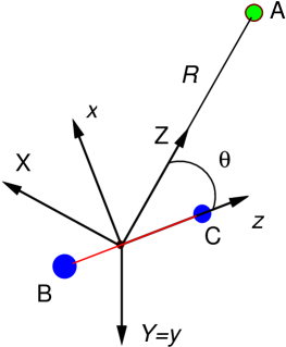
Figure 1: Relative orientation of the molecule-fixed frame ($xyz$) to the space-fixed frame ($XYZ$) with its $Z$ axis directed along the vector ${\mathbf{R}}$ joining the center of mass of the molecule BC and the atom A. The three atoms are in the plane $\sigma_{xz}=\sigma_{XZ}$.

It can easily be shown Nielson:76 that in the case of interaction with an atom in S state the matrix elements $V_{\Lambda,\Lambda}^{(2)}$ and $V_{-\Lambda,-\Lambda}^{(2)}$ are equal, and the same holds for off-diagonal elements $V_{\Lambda,-\Lambda}^{(2)}$ and $V_{-\Lambda,\Lambda}^{(2)}$. The eigenfunctions and the corresponding eigenvalues of the matrix (5) can simply be constructed on the symmetry basis only, as the proper zero-order wave function of the complex AB should have a defined behaviour under the reflection in the plane $\sigma$ containing the three atoms: $\sigma\psi_{AB}^{(+)}=\psi_{AB}^{(+)}$ for A^′ state and $\sigma\psi_{AB}^{(-)}=(-1)\psi_{AB}^{(-)}$ for A^′′ state. In our approach the three atoms lie in the $xz$ plane and the transformation between the space-fixed frame and the body-fixed frames is chosen in such a way that it leads to the coincidence of the axis $y$ in all relevant frames of reference, see Fig. 1. Thus, the symmetry (A^′ or A^′′) of the zero-order wave function $\psi_{AB}^{(\pm)}$ characterizes its behaviour under the reflection in the plane $\sigma_{xz}$. It is determined by the symmetry properties of the wave functions of the two constituent monomers, i.e. $\psi_{A}(\rm S)$ and $\psi_{B}(\Lambda)$, with respect to the reflection in the plane $\sigma_{xz}$ of their body-fixed frames, which happens to be the same. The symmetry relations for the monomer electronic wave functions are ($\Lambda\neq 0$) Roeggen:71 ; Zare :

$$\sigma_{xz}\psi_{B}(\Lambda)=(-1)^{\Lambda}\psi_{B}(-\Lambda),\;\;\sigma_{xz}\psi_{A}({\rm S})=(-1)^{p_{A}}\psi_{A}(\rm S),$$ (8)

where $p_{A}$ defines the spatial parity of the atomic wavefunction in the S state. Therefore, the properly adapted wave functions read:

$$\psi_{AB}^{(\pm)}=\frac{1}{\sqrt{2}}\left[\psi_{A}({\rm S})\psi_{B}(\Lambda)+(-1)^{\Lambda+p_{A}+f}\psi_{A}({\rm S})\psi_{B}(-\Lambda)\right].$$ (9)

and the corresponding second-order energies (i.e. eigenvalues of the matrix $\bm{V}^{(2)}$) are

$$E^{(2)}_{(\pm)}=V_{\Lambda,\Lambda}^{(2)}+(-1)^{\Lambda+p_{A}+f}V_{\Lambda,-\Lambda}^{(2)}$$ (10)

with $f=0$ for A^′ and $f=1$ for A^′′ state. A standard phase convention of Condon and Shortley Condon was adopted to define $\psi_{B}(\Lambda)$ and $\psi_{B}(-\Lambda)$. More details on the symmetry properties of the electronic wave funcions of diatomic molecules can be found in Refs. Roeggen:71 ; Zare ; Pack:70 . Here we only want to conclude that in the case of the systems under study the A^′ state corresponds to the combination of the two terms with the minus sing in Eqs. (9) and (10) for Rb+OH(${}^{2}\Pi$), Rb+CO(${}^{3}\Pi$) and Li+CH(${}^{2}\Pi$) , while the A^′ state has the plus sign for Rb+NH(${}^{1}\Delta$). The opposite holds for the A^′′ states.

The multipole expansion of $V_{\Lambda,\Lambda^{\prime}}$ is readily obtained by inserting the multipole expansion (2) of the interaction operator $V$ into Eq. (7) and collecting terms, as it was done in Refs. Wormer:77 ; Avoird:80 ; Heijmen:96 . Specifically, the derivation is based on the well known transformation properties of the multipole operators from the space-fixed (with the index $m_{X}$) to the body-fixed (with the index $k_{X}$) frame of each monomer (X=A or B):

$$\widehat{Q}_{l_{X}}^{m_{X}}=\sum_{k_{X}=-l_{X}}^{l_{X}}D^{(l_{X})^{\star}}_{m_{X},k_{X}}(\widehat{R}_{X})\widehat{Q}_{l_{X}}^{k_{X}},$$ (11)

where $D^{(l_{X})^{\star}}_{m_{X},k_{X}}(\widehat{R}_{X})$ is the Wigner $D$ matrix, and on the addition theorems for the $D$ functions and spherical harmonics:

$$D^{(l_{X})^{\star}}_{m_{X},k_{X}}(\widehat{R}_{X})\cdot D^{(l_{X}^{\prime})^{\star}}_{m_{X}^{\prime},k_{X}^{\prime}}(\widehat{R}_{X}) =\sum_{L_{X}}\sum_{K_{X}=-L_{X}}^{L_{X}}\sum_{M_{X}=-L_{X}}^{L_{X}}\langle l_{X},k_{X};l_{X}^{\prime},k_{X}^{\prime}|L_{X},K_{X}\rangle$$ (13)

$$\times\langle l_{X},m_{X};l_{X}^{\prime},m_{X}^{\prime}|L_{X},M_{X}\rangle D^{(L_{X})^{\star}}_{M_{X},K_{X}}(\widehat{R}_{X}),$$

$$Y_{l_{A}+l_{B}}^{-m}(\widehat{R})\cdot Y_{l_{A^{\prime}}+l_{B^{\prime}}}^{-m^{\prime}}(\widehat{R}) =\sum_{L}\sum_{M=-L}^{L}\left[\frac{(2l_{A}+2lB+1)(2l_{A^{\prime}}+2l_{B^{\prime}}+1)}{4\pi(2L+1)}\right]^{1/2}$$ (16)

$$\times\langle l_{A}+l_{B},-m;l_{A^{\prime}}+l_{B^{\prime}},-m^{\prime}|L,M\rangle\langle l_{A}+l_{B},0;l_{A}^{\prime}+l_{B}^{\prime},0|L,0\rangle$$

$$\times Y_{L}^{M}(\widehat{R}).$$

The sets of the Euler angles $\widehat{R}_{A}$ and $\widehat{R}_{B}$ describe rotations of the space-fixed frame to the appropriate body-fixed frames. For our convinience we choose the $Z$ axis along the intermolecular axis connecting the two centers of mass. Then, the angular factor $Y_{L}^{M}(\widehat{R})$ reduces to:

$$Y_{L}^{M}(\widehat{R})=Y_{L}^{M}(0,\phi)=\left(\frac{2L+1}{4\pi}\right)^{1/2}\delta_{M,0}.$$ (17)

For an atom in an S state the quantum numbers $L_{A}$, $M_{A}$ and $K_{A}$ are zero, so $D^{(L_{A})^{\star}}_{M_{A},K_{A}}(\widehat{R}_{A})=1$. For an open-shell linear molecule we have $M_{B}=0$, and the set of the three Euler angles is $\widehat{R}_{B}=(0,\theta,0)$, so

$$D^{(L_{B})^{\star}}_{0,K_{B}}(0,\theta,0)=(-1)^{K_{B}}\sqrt{\frac{(L_{B}-K_{B})!}{(L_{B}+K_{B})!}}P^{K_{B}}_{L_{B}}(\cos\theta)$$ (18)

where $P^{K_{B}}_{L_{B}}(\cos\theta)$ denotes the associated Legendre polynomial. The set of the Euler angles $\widehat{R}_{B}=(0,\theta,0)$ for a linear molecule is consistent with the foregoing requirement of the coincidence of the axis $y$ in all relevant frames of reference, cf. Fig. 1. The other possible set would be $\widehat{R}_{B}=(3\pi/2,\theta,\pi/2)$ which leads to the coincidence of the axis $x$ as it was adopted in Ref. Nielson:76 .

It is useful to express the final equations for the elements of the matrix $\mathbf{V}^{(2)}$ in terms of the static and dynamic multipole polarizabilities of the atom and molecule. For an S atom we use the standard definition:

$$\alpha^{ll^{\prime}}_{mm^{\prime}}(\omega)=2\sum_{\{k\}}{{}^{\prime}}\;\omega_{{\rm S},k}\frac{\langle\psi_{A}({\rm S})|\widehat{Q}_{l}^{m}|\psi_{A}(\{k\})\rangle\langle\psi_{A}(\{k\})|\widehat{Q}_{l^{\prime}}^{m^{\prime}}|\psi_{A}({\rm S})\rangle}{\omega_{{\rm S},k}^{2}-\omega^{2}},$$ (19)

while for an open-shell linear molecule we introduce extra superscripts $\Lambda$ and $\Lambda^{\prime}$ to distinguish between diagonal and off-diagonal components:

$${}^{\Lambda,\Lambda^{\prime}}\alpha^{ll^{\prime}}_{mm^{\prime}}(\omega)=2\sum_{\{n\}}{{}^{\prime}}\;\omega_{\Lambda,n}\frac{\langle\psi_{B}(\Lambda)|\widehat{Q}_{l}^{m}|\psi_{B}(\{n\})\rangle\langle\psi_{B}(\{n\})|\widehat{Q}_{l^{\prime}}^{m^{\prime}}|\psi_{B}(\Lambda^{\prime})\rangle}{\omega_{\Lambda,n}^{2}-\omega^{2}}.$$ (20)

The corresponding irreducible polarizabilities are obtained by Clebsch-Gordan coupling:

$${}^{(\Lambda,\Lambda^{\prime})}\alpha^{(ll^{\prime})L}_{K}(\omega)=\sum_{m,m^{\prime}}\langle l,m;l^{\prime},m^{\prime}|L,K\rangle^{(\Lambda,\Lambda^{\prime})}\alpha^{ll^{\prime}}_{mm^{\prime}}(\omega).$$ (21)

The only nonvanishing components of the irreducible polarizability for an atom in the S state are $\alpha^{(ll)0}_{0}$, while for an open-shell linear molecule the nonzero components are ${}^{\Lambda,\Lambda^{\prime}}\alpha^{(ll^{\prime})L}_{K}$ with $K=0$ for $\Lambda=\Lambda^{\prime}$ and with $K=2\Lambda$ if $\Lambda^{\prime}=-\Lambda$.

We are now ready to give final expressions for the long-range coefficients expressed in terms of the irreducible components of the polarizabilities:

$$V_{\Lambda,\Lambda^{\prime}}^{(2)}=-\sum_{l_{A},l_{B},l_{B}^{\prime}}\sum_{L,K}\xi^{L,K}_{l_{A}l_{B}l_{B}^{\prime}}R^{-(2+2l_{A}+l_{B}+l_{B}^{\prime})}\left[{}^{\Lambda,\Lambda^{\prime}}C_{l_{A}l_{B}l_{B}^{\prime}}^{L,K}({\rm ind})+\;{{}^{\Lambda,\Lambda^{\prime}}C_{l_{A}l_{B}l_{B}^{\prime}}^{L,K}}({\rm disp})\right]P_{L}^{|K|}(\cos\theta),$$ (22)

where the constant $\xi^{L,K}_{l_{A}l_{B}l_{B}^{\prime}}$ is given by:

$$\xi_{l_{A}l_{B}l_{B}^{\prime}}^{L,K} =\left[\frac{(2l_{A}+2l_{B}+1)!(2l_{A}+2l_{B^{\prime}}+1)!}{(2l_{A})!(2l_{B})!(2l_{A})!(2l_{B^{\prime}})!}\right]^{1/2}\pmatrix{l_{A}+l_{B}&l_{A}+l_{B}^{\prime}&L\cr 0&0&0\cr}$$ (26)

$$\times\left(\frac{2L+1}{2l_{A}+1}\right)^{1/2}\sqrt{\frac{(L-K)!}{(L+K)!}}\left\{\begin{array}[]{ccc}l_{B}&l_{A}+l_{B}&l_{A}\\ l_{A}+l_{B}^{\prime}&l_{B}^{\prime}&L\end{array}\right\},$$

and the expressions in the round and curly brackets are the $3j$ and $6j$ coefficients, respectively. Combining all terms with the same power $n=2l_{A}+l_{B}+l_{B}^{\prime}+2$ in the above expansion, we will get standard long-range coefficients $C_{n}^{L,K}$:

$$C_{n}^{L,K}=\sum_{l_{A},l_{B},l_{B}^{\prime}}^{2l_{A}+l_{B}+l_{B}^{\prime}+2=n}\xi^{L,K}_{l_{A}l_{B}l_{B}^{\prime}}\left[{{}^{\Lambda,\Lambda^{\prime}}}C_{l_{A}l_{B}l_{B}^{\prime}}^{L,K}({\rm ind})+\;{{}^{\Lambda,\Lambda^{\prime}}}C_{l_{A}l_{B}l_{B}^{\prime}}^{L,K}({\rm disp})\right],$$ (27)

by means of which the asymptotic expansion of Eq. (10) simply reads:

$$E^{(2)}_{(\pm)}=-\sum_{n=6}^{\infty}\sum_{L}\left[\frac{C_{n}^{L,0}}{R^{n}}P_{L}^{0}(\cos\theta)+(-1)^{\Lambda+p_{A}+f}\frac{C_{n}^{L,2\Lambda}}{R^{n}}P_{L}^{|2\Lambda|}(\cos\theta)\right].$$ (28)

The dipersion part ${}^{\Lambda,\Lambda^{\prime}}C_{l_{A}l_{B}l_{B}^{\prime}}^{L,K}({\rm disp})$ is proportional to the Casimir-Polder integral over the atomic and molecular polarizabilities calculated at imaginary frequencies:

$${}^{\Lambda,\Lambda^{\prime}}C_{l_{A}l_{B}l_{B}^{\prime}}^{L,K}({\rm disp})=\frac{1}{2\pi}\int_{0}^{\infty}\alpha^{(l_{A}l_{A})0}_{0}(i\omega)\;{{}^{\Lambda,\Lambda^{\prime}}\alpha^{(l_{B}l_{B}^{\prime})L}_{K}}(i\omega){\rm d}\omega,$$ (29)

while the induction term ${}^{\Lambda,\Lambda^{\prime}}C_{l_{A}l_{B}l_{B}^{\prime}}^{L,K}({\rm ind})$ is the product of the static polarizability of the atom and permanent multipole moments of the open-shell molecule:

$${}^{\Lambda,\Lambda^{\prime}}C_{l_{A}l_{B}l_{B}^{\prime}}^{L,K}({\rm ind})=\alpha^{(l_{A}l_{A})0}_{0}(0)\left[\langle\psi_{B}(\Lambda)|\widehat{Q}_{l_{B}}|\psi_{B}(\pm|\Lambda|)\rangle\otimes\langle\psi_{B}(\pm|\Lambda|)|\widehat{Q}_{l_{B}^{\prime}}|\psi_{B}(\Lambda^{\prime})\rangle\right]_{K}^{L}.$$ (30)

A few comments are needed here. The expression for the diagonal term $V^{(2)}_{\Lambda,\Lambda}$ is the same as for the interaction between atom and linear molecule in a spatially nondegenerate state ($\Sigma$). The additional term emerging when $\Lambda\neq 0$ is the off-diagonal $V^{(2)}_{\Lambda,-\Lambda}$. It has both induction and dispersion parts. As it was already stated, the only nonvanishing term in $V^{(2)}_{\Lambda,-\Lambda}$ appears for $K=2\Lambda$. The lowest order long-range coefficient, to which the off-diagonal term contributes to, is $C_{n}^{L,K}$ with $n=4+2|\Lambda|$ for the dispersion part and $n=5+2|\Lambda|$ for the induction part. The source of the induction energy in $V^{(2)}_{\Lambda,-\Lambda}$ comes from the fact that open-shell linear molecules have an additional independent component of the permanent multipole moments, $\langle\psi(\Lambda)|\widehat{Q}^{2\Lambda}_{l}|\psi(-\Lambda)\rangle$, in contrast to the $\Sigma$ state molecules with only one independent component, namely $\langle\psi(\Lambda)|\widehat{Q}^{0}_{l}|\psi(\Lambda)\rangle$. It is obvious that the second independent component appears for $l\geq 2|\Lambda|$, therefore in the case of the $\Pi$ states there is no induction contribution to the off-diagonal $C_{6}^{2,2}$ coefficient. The dispersion terms in $V^{(2)}_{\Lambda,-\Lambda}$ results from the presence of additional components of the polarizability terms for the open-shell linear molecules.

In general, the number of independent diagonal terms ${}^{\Lambda,\Lambda}\alpha^{ll^{\prime}}_{kk^{\prime}}$ is equal to $2l_{<}+1$ (where $l_{<}$ is the smaller of $l$ and $l^{\prime}$). Each of the non-redundant components ${}^{\Lambda,\Lambda}\alpha^{ll^{\prime}}_{kk^{\prime}}$ comes from the transitions in the sum (20) through the intermediate states $\psi(\{n\})$ with the projection of the eletronic angular momentum ranging $|\Lambda|-(2l_{<}+1)$ to $|\Lambda|+(2l_{<}+1)$. Due to the transformation properties, the number of independent irreducible components ${}^{\Lambda,\Lambda}\alpha^{(ll^{\prime})L}_{K}$ will also be $2l_{<}+1$.

In addition, for open-shell linear molecules, there are nondiagonal components of the polarizability tensor ${}^{\Lambda,-\Lambda}\alpha^{ll^{\prime}}_{kk^{\prime}}$ which do not vanish, and are not related to the diagonal terms. The nondiagonal terms in the multipole polarizability tensor appear if the condition $k^{\prime}+k=2\Lambda$ can be fulfilled for a given set of the quantum numbers $(l,k)$ and $(l^{\prime},k^{\prime})$. They result from the fact that there are transitions through the same operator to states $\Sigma^{+}$ and $\Sigma^{-}$, and then ${}^{\Lambda,-\Lambda}\alpha^{ll^{\prime}}_{kk}$ is the diffrence between these two separate contributions (e.g. ${}^{1,1}\alpha^{11}_{11}$ for the $\Pi$ state). The other mechanism leading to the appearance of the nondiagonal ${}^{\Lambda,-\Lambda}\alpha^{ll^{\prime}}_{kk^{\prime}}$ terms is parallel with the source of the off-diagonal induction terms, namely there are possible two independent transition moments between the state in question $|\psi(\Lambda)\rangle$ and the exited states through an operator of the same rank, e.g. ${}^{1,-1}\alpha^{12}_{02}$ for the $\Pi$ state, to be compared with the diagonal ${}^{1,1}\alpha^{12}_{00}$ .

Let us discuss the dipole polarizabilities in more details. For open-shell diatomic molecules there are three independent spherical components ${}^{\Lambda,\Lambda}\alpha^{11}_{kk^{\prime}}$ with $(k,k^{\prime})$ equal to $(0,0)$, $(1,-1)$ and $(-1,1)$, the corresponding transitions in sum-over-states occur through the excited states with a projection of electronic angular momentum equal to $\Lambda$, $\Lambda-1$, and $\Lambda+1$, respectively. In case of the $\Pi$ states there is extra nondiagonal component ${}^{1,-1}\alpha^{11}_{11}$ with intermediate states $\Sigma^{+}$ and $\Sigma^{-}$ in the sum-over-state expression, which come with opposite sign, in contrast to ${}^{1,1}\alpha^{11}_{-11}$ in which states $\Sigma^{+}$ and $\Sigma^{-}$ contribute with the same sign. The four corresponding irreducible dipole polarizability components would be ${}^{\Lambda,\Lambda}\alpha^{(11)0}_{0}$, ${}^{\Lambda,\Lambda}\alpha^{(11)2}_{0}$, ${}^{\Lambda,\Lambda}\alpha^{(11)1}_{0}$, and ${}^{\Lambda,-\Lambda}\alpha^{(11)2}_{2}$, the last one is nonvanishing only for the $\Pi$ states.

From the analysis of Eq. (22) it turns out that not all nonvanishing irreducible components ${}^{\Lambda,\Lambda^{\prime}}\alpha^{(ll^{\prime})L}_{K}$ of the molecule polarizability tensor are needed to express the interaction energy of an open-shell linear molecule with an atom. The dipole component ${}^{\Lambda,\Lambda}\alpha^{(11)1}_{0}$ is redundant in this case. It follows from the expression (26) that all terms ${}^{\Lambda,\Lambda^{\prime}}\alpha^{(ll^{\prime})L}_{K}$ with $l+l^{\prime}+L$ odd do not contribute to the interaction energy in the second order $E_{(\pm)}^{(2)}$. However, if we had an asymetric molecule or an other linear open-shell species instead of an atom then all non-zero irreducible componets would be necessary. For a $\Delta$ state there are three independent dipole polarizabilities, but again, in the case of interaction with an atom, ${}^{2,2}\alpha^{(11)1}_{0}$ is redundant. The first off-diagonal term for a $\Delta$ state will be ${}^{2,-2}\alpha^{(22)4}_{4}$ or equivalently ${}^{2,-2}\alpha^{22}_{22}$.

Sometimes it is more convenient to use the Cartesian basis both for the states $|\Lambda\rangle$ and multipole moments. The transformation formulas between the two bases can be found in Ref. Gray:75 . We focus again on the $\Pi$ states. In the Cartesian basis the two degenerate states $|\pm 1\rangle$ are usually referred to as $|\Pi_{\rm{x}}\rangle$ and $|\Pi_{\rm{y}}\rangle$. The four independent dipole polarizability tensor components would be ${}^{\rm{x,x}}\alpha_{\rm{xx}}$, ${}^{\rm{x,x}}\alpha_{\rm{yy}}$, ${}^{\rm{x,x}}\alpha_{\rm{zz}}$, and ${}^{\rm{x,y}}\alpha_{\rm{xy}}$, where we adopted the index (x,y) in place of (-1,1) to distinguish between particular diagonal and off-diagonal components. It is possible to define the fifth Cartesian component, namely ${}^{\rm{x,y}}\alpha_{\rm{yx}}$, however, due to the relation: ${}^{\rm{x,x}}\alpha_{\rm{xx}}-{{}^{\rm{x,x}}}\alpha_{\rm{yy}}={{}^{\rm{x,y}}}\alpha_{\rm{xy}}+{{}^{\rm{x,y}}}\alpha_{\rm{yx}}$, it will not be independent Spelsberg:99 . To see better why the Cartesian basis may be useful let us mention how the irreducible spherical components are related to the Cartesian ones for the $\Pi$ states:

$${}^{1,1}\alpha^{(1,1)0}_{0} =^{-1,-1}\alpha^{(1,1)0}_{0}=-\frac{1}{\sqrt{3}}\left({{}^{\rm{x,x}}}\alpha_{\rm{xx}}+{{}^{\rm{x,x}}}\alpha_{\rm{yy}}+{{}^{\rm{x,x}}}\alpha_{\rm{zz}}\right)$$ (31)

$${}^{1,1}\alpha^{(1,1)2}_{0} =^{-1,-1}\alpha^{(1,1)2}_{0}=\frac{1}{\sqrt{6}}\left(2\;{{}^{\rm{x,x}}}\alpha_{\rm{zz}}-{{}^{\rm{x,x}}}\alpha_{\rm{xx}}-{{}^{\rm{x,x}}}\alpha_{\rm{yy}}\right)$$ (32)

$${}^{1,1}\alpha^{(1,1)1}_{0} =-^{-1,-1}\alpha^{(1,1)1}_{0}=-\frac{1}{\sqrt{2}}\left({{}^{\rm{x,y}}}\alpha_{\rm{xy}}-{{}^{\rm{x,y}}}\alpha_{\rm{yx}}\right)$$ (33)

$${}^{1,-1}\alpha^{(1,1)2}_{2} =^{-1,1}\alpha^{(1,1)2}_{-2}={{}^{\rm{x,x}}}\alpha_{\rm{yy}}-{{}^{\rm{x,x}}}\alpha_{\rm{xx}}$$ (34)

An inspection of the above relations shows that in order to express the interaction energy of a $\Pi$ molecule with an atom, only diagonal Cartesian components are needed, as the off-diagonal ${{}^{\rm{x,y}}}\alpha_{\rm{xy}}$ contributes only to ${}^{1,1}\alpha^{(1,1)1}_{0}$, i.e. the term not present in expression for $E^{(2)}_{(\pm)}$. The off-diagonal irreducible component ${}^{1,-1}\alpha^{(1,1)2}_{2}$ is equal to the difference between two perpendicular $\alpha$’s calculated for one of the Cartesian states. This observation is more general and it turns out that if we decide for a Cartesian representation of the $|\Lambda\rangle$ states, then all off-diagonal irreducible components ${}^{\Lambda,-\Lambda}\alpha^{(ll^{\prime})L}_{2\Lambda}$ can be related to some diagonal Cartesian terms. Still, we will have to calculate some additional Cartesian components, however, diagonal only, which are not present in the expression for the diagonal ${}^{\Lambda,\Lambda}\alpha^{(ll^{\prime})L}_{0}$ terms. Calculations of the off-diagonal polarizability components in the Cartesian basis are indispensable if the interacting system comprises of an open-shell molecule and asymmetric species. It means that in such a case the interaction energy in the multipole approximation is expressed in terms of, for instance, ${{}^{\rm{x,y}}}\alpha_{\rm{xy}}$ component. It is worth noting that ${{}^{\rm{x,y}}}\alpha_{\rm{xy}}$ is irrelevant in the describtion of the interaction of the open-shell molecule with the extrenal electric field in the Stark effect. Thus, the induction energy and, consequently, intermolecular forces explores properties of the open-shell diatomic molecules which are not accessible otherwise.

Note that Eq. (29) is strictly valid only when the molecule is in its ground electronic state. If the molecule is in an excited state that is connected to the ground state (or to any other state lower in energy) by multipolar transition moments then the Casimir-Polder integral is no longer valid and an extra term has to be added to the energy. The reason behind this is the property of the Casimir-Polder integral that if the two elements in denominator, $\epsilon_{A}$ and $\epsilon_{B}$, have opposite signs then we obtain (assuming that $\epsilon_{B}<0$):

$$\frac{2}{\pi}\int_{0}^{\infty}\frac{\epsilon_{A}}{\epsilon_{A}^{2}+\omega^{2}}\cdot\frac{\epsilon_{B}}{\epsilon_{B}^{2}+\omega^{2}}{\rm d}\omega=-\frac{1}{\epsilon_{A}+|\epsilon_{B}|},$$ (35)

instead of the value of $1/(\epsilon_{A}-|\epsilon_{B}|)$, which we want to decompose into the product of two terms depending on monomer properties only. Formally, we may write the following identity (again $\epsilon_{B}<0$):

$$\frac{1}{\epsilon_{A}-|\epsilon_{B}|}=\frac{2}{\pi}\int_{0}^{\infty}\frac{\epsilon_{A}}{\epsilon_{A}^{2}+\omega^{2}}\cdot\frac{\epsilon_{B}}{\epsilon_{B}^{2}+\omega^{2}}{\rm d}\omega+\frac{1}{\epsilon_{A}+|\epsilon_{B}|}+\frac{1}{\epsilon_{A}-|\epsilon_{B}|}.$$ (36)

For any molecular state with $\epsilon_{B}<0$ we have the summation (7) over all atomic states with positive excitation energy $\epsilon_{A}$, this means that the two last factors in the above equation will add up to yield dynamic polarizability of atom at frequency $\omega=|\epsilon_{B}|$. Therefore, if we want to express the whole interaction energy in the second order $E^{(2)}_{(\pm)}$ in terms of the monomers properties only, then we are forced to add an extra term to the dispersion part, Eq. (29), in order to compensate an error introduced by the integral representation of the dispersion energy. This additional term depends on the dynamic polarizabilites of the atom calculated at frequency $\omega$ equal to the energy of all possible deexcitations in the molecule, and will be denoted by $C_{l_{A}l_{B}l_{B}^{\prime}}^{L,K}({\rm corr,deexc})$. Its form is slightly similar to the induction part:

$${}^{\Lambda,\Lambda^{\prime}}C_{l_{A}l_{B}l_{B}^{\prime}}^{L,K}({\rm corr,deexc}) =\sum_{\{n^{-}\}}\alpha^{(l_{A}l_{A})0}_{0}(\omega_{n^{-},\Lambda})$$ (38)

$$\times\left[\langle\psi_{B}(\Lambda)|\widehat{Q}_{l_{B}}|\psi_{B}(\{n^{-}\})\rangle\otimes\langle\psi_{B}(\{n^{-}\})|\widehat{Q}_{l_{B}^{\prime}}|\psi_{B}(\Lambda^{\prime})\rangle\right]_{K}^{L}.$$

The summation in the above equation runs only over states of the molecule $\psi_{B}(\{n^{-}\})$ with energy lower than the reference one, i.e. if $\omega_{n^{-},\Lambda}=E_{\Lambda}-E_{\{n^{-}\}}$ is positive, and hence $\omega_{n^{-},\Lambda}$ corresponds to the possible deexcitations of the molecule. This term does not have a simple physical interpretation, but as shown in Ref. skomo it leads to a different QED retardation of the long-range potential than given by the classical Casimir-Polder formula Polder:48 . Note also that without this extra term, the second-order interaction energy in the long-range could not be written correctly in terms of molecular properties of the isolated subsystems in the case when deexcitation may occur. Obviously, a similar term will be needed if an atom is in an exited state and molecule in its ground state. Then $C_{l_{A}l_{B}l_{B}^{\prime}}^{L,K}({\rm corr,deexc})$ would depend on the the dynamic polarizabilities of the molecule at frequency $\omega$ corresponding to possible atomic deexcitation. However, this holds only for atomic excited S states, as if the atomic state was P, D etc. then the whole formalism presented here would not be longer valid due to nonvanishing first-order energy in the multipole approximation.

III Numerical results and discussion

We have applied the theory exposed above to the interactions of the ground state rubidium atom Rb(²S) with CO(${}^{3}\Pi$), OH(${}^{2}\Pi$), NH(${}^{1}\Delta$), and CH(${}^{2}\Pi$), and of the ground state lithium atom Li(²S) with CH(${}^{2}\Pi$). As discussed in the Introduction, these molecules have been successfully decelerated and are the best candidates for sympathetic cooling by collisions with ultracold rubidium atoms. At present no ab initio code allows for the calculations of all components of the dynamic polarizability tensor for open-shell linear molecules. Therefore, in our calculations we computed the polarizabilities appearing in Eqs. (30) and (29), from the sum-over-states expansion, Eq. (20). The appropriate transitions moments to the excited states and excitation energies were calculated using linear response formalism with reference wave function obtained from the multireference selfconsistent field method (MCSCF) with large active spaces. For some electronic states the convergence of the sum in Eq. (20) was not very fast, and we had to include over 100 states in the expansion. The dalton program was used for linear response calculations. We have checked the convergence of the expansion (20) by comparison of the static parallel components obtained from the MCSCF calculations with the results of finite-field restricted open-shell coupled cluster calculations with single, double, and noniterative triple excitations, RCCSD(T). The finite field calculations were done with the molpro code molpro . Note parenthetically that finite field calculations can correctly reproduce the parallel component of the polarizability tensor, but fail for the perpendicular component due to the symmetry breaking. The nondiagonal components cannot be obtained from finite-field calculations. We have attempted to use the multiconfiguration interaction method restricted to single and double excitations (MRCI), but due to the convergence problems, we could get in this way only a few (up to ten) excited states. The Li and Rb atoms polarizabilities at imaginary frequency was taken from highly accurate relativistic calculations from the group of Derevianko Derevianko:10 .

In order to judge the quality of the computed long-range coefficients we have computed cuts through the potential energy surfaces of Rb–CH(${}^{2}\Pi$) at a fixed distance $R$=30 bohr from the atom to the center of mass of the molecule. The zero of the angle $\theta$ corresponds to the rubidium atom on the H side of CH. In these calculations we have employed the supermolecule method. The potential was computed as the difference,

$$V^{\rm{}^{2S+1}|\Lambda|}(R,\theta)=E_{\rm AB}^{\rm SM}-E_{\rm A}^{\rm SM}-E_{\rm B}^{\rm SM},$$ (39)

where $E_{\rm AB}^{\rm SM}$ denotes the energy of the dimer computed using the supermolecule method SM, and $E_{\rm X}^{\rm SM}$, X=A or B, is the energy of the atom X. For the high-spin states (triplet for Rb(²S)–OH(${}^{2}\Pi$), Rb(²S)–CH(${}^{2}\Pi$), and Li(²S)–CH(${}^{2}\Pi$), quartet for Rb(²S)–CO(${}^{3}\Pi$), and doublet for Rb(²S)–NH(${}^{1}\Delta$) we used the restricted open-shell coupled cluster method restricted to single, double, and noniterative triple excitations [RCCSD(T)]. Since the low-spin states have the same asymptotic behavior as the high-spin states there was no need to compute the ab initio points explicitly. The RCCSD(T) calculations were done with the molpro suite of codes molpro . The distances in the diatomic molecules were fixed at their equilibrium values $r_{e}$ corresponding to the electronic state considered. For CO(${}^{3}\Pi$) $r_{e}$ was set equal to 2.279 bohr, for OH(${}^{2}\Pi$) 1.834 bohr, for NH(${}^{1}\Delta$) 1.954 bohr, and 2.116 bohr for CH(${}^{2}\Pi$) nistpage . The angle $\theta=0^{\circ}$ corresponds to the linear geometris CH–Rb, CH–Li, OH–Rb, NH–Rb and CO–Rb. In order to mimic the scalar relativistic effects some electrons were described by pseudopotentials. For rubidium we took the ECP28MDF pseudopotential from the Stuttgart library Stoll:05 , and the $spdfg$ quality basis set suggested in Ref. Stoll:05 . For the light atoms (hydrogen, carbon, nitrogen, and oxygen) we used the aug-cc-pVQZ bases Dunning:94 . The full basis of the dimer was used in the supermolecule calculations and the Boys and Bernardi scheme was used to correct for the basis-set superposition error Boys:71 .

Before going on with the discussion of the long-range interactions in the dimers, let us compare the diagonal static polarizabilities of CO(${}^{3}\Pi$), OH(${}^{2}\Pi$), NH(${}^{1}\Delta$), and CH(${}^{2}\Pi$) with the literature data. In fact, the data are very scarce. For OH the most recent calculations of Spelsberg Spelsberg:99 date back to 1999 (see also some older references Adamowicz:88 ; Dinur:94 ; Karna:96 ). For CH the only calculation we found in the literature is the 2007 paper by Manohar and Pal Pal:07 . To our knowledge no data for the excited states of CO and NH were reported thus far. An ispection of Table 1 shows a relatively good agreement with the results of Spelsberg Spelsberg:99 for OH. The differences are of the order of a few percent, 5.5% for the parallel component, and 6.3% and 3.3% for the perpendicular $xx$ and $yy$ components, respectively. For CH Manohar and Pal Pal:07 reported only the value of the parallel component obtained from the analytical second derivative calculations with the Fock space multireference coupled cluster theory restricted to single and double excitations. The agreement of our result with the value of Ref. Pal:07 is remarkably good: the two results agree within 0.4%.

The long-range coefficients $C_{n}^{L,K}$ for the interactions of the ground state rubidium atom Rb(²S) with CO(${}^{3}\Pi$), OH(${}^{2}\Pi$), NH(${}^{1}\Delta$), and CH(${}^{2}\Pi$), and of the ground state lithium atom Li(²S) with CH(${}^{2}\Pi$) are reported in Tables 2–6. Also reported in these tables are the values of the induction and dispersion coefficients $C_{n}^{L,K}({\rm ind})$ and $C_{n}^{L,K}({\rm disp})$. First we note that for all systems and most of the coefficients the induction part is as important as the dispersion. This is not very surprising since the Li and Rb atoms are highly polarizable, and the molecules suitable for the Stark deceleration have large dipole moments. Note parenthetically that the coefficient $C_{6}^{22}({\rm ind})$ for the interactions of the $\Pi$ state molecules and $C_{8}^{24}({\rm ind})$ for the interactions of the $\Delta$ state molecules vanish for symmetry reasons. The leading contribution to the anisotropy of the potentials in the long range, as measured by the ratio $C_{6}^{20}/C_{6}^{00}$, is quite substantial for all the systems. The ratio $C_{6}^{20}/C_{6}^{00}$ ranges between 0.26 for Li–CH and Rb–CH to 0.43 for Rb–OH. The difference in the anisotropy due to the presence of terms $C_{n}^{L2}/R^{n}$ is relatively modest, since the coefficients $C_{n}^{L2}$ are at least one order of magnitude smaller than $C_{n}^{L0}$.

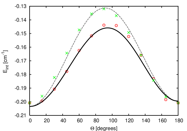
Figure 2: Comparison of the long-range anisotropy of the potential energy surfaces for the doublet and quartet A^′ (solid line vs. circles) and A^′′ (dotted line vs. crosses) states of Rb–CH(${}^{2}\Pi$) computed from the mutlipole expansion up to and including $R^{-10}$ and from the supermolecule calculations.

Comparison of the long-range anisotropy of the potential energy surfaces for the singlet and triplet A^′ and A^′′ states of Rb–CH(${}^{2}\Pi$) computed from the mutlipole expansion up to and including $R^{-10}$ and from the supermolecule calculations is illustrated in Fig. 2. The agreement between the long-range and supermolecule results is relatively good, although small deviations can be observed. For the A^′ state the agreement is good at small angles, and slightly deteriorates for $\theta$ around 100^∘. The same is true for the A^′′ state, showing that our computed coefficients are not the perfect representation of the asymptotic expansion of the RCCSD(T) potential for this system. It should be stressed here that the long-range coefficients reported in the present paper do not describe the asymptotics of any potential obtained from supermolecule calculations, since for most of the supermolecule methods the long-range asymptotics is not known. See, e.g. Ref. Moszynski:99 for a more detailed discussion of this point. However, the data reported in the present paper can be used in the fits of the potentials, or in the case of lack of ab initio points at large distances, to fix the long-range asymptotics with some switching function liesbeth .

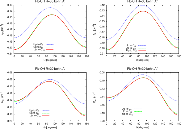
Figure 3: Importance of the $R^{-6}$, $R^{-8}$, and $R^{-10}$ contributions to the long-range anisotropy of the potential energy surfaces for the A^′ and A^′′ states of Rb–CH(${}^{2}\Pi$) and Rb–OH(${}^{2}\Pi$) computed from the mutlipole expansion.

To illustrate the importance of the long-range coefficients with $n>6$ in Fig. 3 we report cuts through the potential energy surfaces of the least (Rb–CH) and most (Rb–OH) anisotropic systems for a fixed distance $R=30$ bohr. An inspection of this figure shows that the contribution of the coefficients beyond $n=6$ is very important. For Rb–CH the $R^{-6}$ terms qualitatively reproduce the anisotropy of the potential. This is not the case for Rb–OH. The inclusion of all terms up to $n=8$ gives the correct picture of the anisotropy, and the $R^{-9}$ and $R^{-10}$ contributions are of minor importance at this distance. It follows from the comparison of the RCCSD(T) results with the data computed from the asymptotic expansion, cf. Fig. 2, that the short-range exchange-repulsion effects are negligible at this distance. Thus, our illustration of Fig. 3 trully demonstrates the importance of the $R^{-8}$ and higher terms in the multipole expansion of the interaction energy. Obviously, the importance of the contributions beyond the $C_{6}$ depends on the distance $R$, but our plot clearly shows that in the region of negligible exchange and overlap the contributions beyond $C_{6}$ are important.

No literature data are available for comparison, except for the long-range coefficients for Rb–OH obtained by Lara et al. Lara:07 by fitting the CCSD(T) potential energy surfaces in the A^′ and A^′′ symmetries at large distances to the functional form of Eq. (22). The values of the long-range coefficients taken from Ref. Lara:07 are included in Table 3. The agreement between the two sets of the results is very reasonable. The isotropic $C_{6}^{00}$ coefficients agree within 7%. The discrepancies of the anisotropic coefficients are of the order of 10 to 15%. Such an agreement is satisfactory given the fact that the fitted values effectively account for the higher coefficients that could not be obtained from the fit. The only significant difference is in $C_{6}^{22}$. Here the difference is as large as 37%, but this coefficient is small, and most probably could not be correctly reproduced from the fitting procedure. By contrast, the values of $C_{7}^{32}$ agree relatively well, within 10%.

Hutson priv estimated the lowest dispersion coefficients $C_{6}^{00}$, $C_{6}^{20}$, and $C_{6}^{22}$ for Rb–OH by using the best available data for the static polarizability of Rb and OH, and the Slater-Kirkwood rules. He obtained an isotropic $C_{6}^{00}$ coefficient of 149.4 a.u., 30% off our value. Such an agreement is reasonable given all the simplifications of the Slater-Kirkwood approach. The values of the anisotropic coefficients $C_{6}^{20}$ and $C_{6}^{22}$, 4.3 and 0.9 a.u., respectively are four and three times smaller than those reported in the present paper, and thus unrealistic. This shows that the applicability of simple semiempirical rules to anisotropic interactions in open-shell complexes is of limited utility. We have performed a similar analysis for other complexes considered in our paper, and came to similar conclusions.

IV Summary and conclusions

In the present paper we have formulated the theory of long-range interactions between a ground-state atom in an S state and a linear molecule in a degenerate state with a non-zero projection of the electronic orbital angular momentum. We have shown that the long-range coefficients describing the induction and dispersion interactions at large atom–diatom distances can be related to the first and second-order molecular properties. The final expressions for the long-range coefficients were written in terms of all components of the static and dynamic multipole polarizability tensor, including the nonadiagonal terms connecting states with the opposite projection of the electronic orbital angular momentum. It was also shown that for the interactions of molecules in excited states that are connected to the ground state by multipolar transition moments additional terms in the long-range induction energy appears. All these theoretical developments were illustrated with the numerical results for systems of interest for the sympathetic cooling experiments: interactions of the ground state Rb(²S) atom with CO(${}^{3}\Pi$), OH(${}^{2}\Pi$), NH(${}^{1}\Delta$), and CH(${}^{2}\Pi$), and of the ground state Li(²S) atom with CH(${}^{2}\Pi$). Our results for the static polarizabilities of the OH and CH molecules are in a good agreement with the ab initio data from other authors Spelsberg:99 ; Pal:07 . For all systems considered in the present paper the induction contribution to the long-range potential was found to be important. Also the anisotropy of the long-range interaction, as measured by the ratio $C_{6}^{20}/C_{6}^{00}$, is substantial, while the anisotropy due to the $C_{6}^{22}$ is of modest importance. Relatively good agreement between the multipole-expanded and ab initio RCCSD(T) results was found. In the asymptotic region, where the exchange effects are negligible, terms $R^{-n}$ with $n\geq 8$ are very important, and cannot be neglected. For Rb–OH we could compare our results with the fit of ab initio RCCSD(T) points Lara:07 . In general, relatively good agreement was found, except for the small $C_{6}^{22}$ coefficient. It was also found that the Slater-Kirkwood rules for the anisotropic long-range coefficients fail in the case of open-shell monomers with spatial degeneracy.

Table 1: Diagonal Cartesian components of the static dipole polarizabilities (in a.u.) for CO(${}^{3}\Pi$), OH(${}^{2}\Pi$), NH(${}^{1}\Delta$), and CH(${}^{2}\Pi$).

	CO(${}^{3}\Pi$)	OH(${}^{2}\Pi$)	NH(${}^{1}\Delta$)	CH(${}^{2}\Pi$)	Reference
${}^{{\rm x,x}}\alpha_{zz}$	17.97	8.29	11.23	15.80	present
		8.75			Ref. Spelsberg:99
				15.86	Ref. Pal:07
${}^{{\rm x,x}}\alpha_{xx}$	12.75	5.99	9.15	14.32	present
		6.37			Ref. Spelsberg:99
${}^{{\rm x,x}}\alpha_{yy}$	9.91	7.31	9.15	11.81	present
		7.55			Ref. Spelsberg:99

Table 2: Long-range coefficients (in atomic units) for Rb–CO(${}^{3}\Pi$). $C_{n}^{L,K}$ is the sum $C_{n}^{L,K}({\rm ind})+C_{n}^{L,K}({\rm disp})$. The number in parentheses denotes the power of 10.

$L~{}\rightarrow$	0	1	2	3	4	5	6
$C_{6}^{L0}({\rm ind})$	1.187(2)		1.187(2)
$C_{6}^{L0}({\rm disp})$	3.797(2)		6.400(1)
$C_{6}^{L0}$	4.984(2)		1.827(2)
$C_{6}^{L2}({\rm ind})$			0
$C_{6}^{L2}({\rm disp})$			–1.415(1)
$C_{6}^{L2}$			–1.415(1)
$C_{7}^{L0}({\rm ind})$		4.646(2)		3.103(2)
$C_{7}^{L0}({\rm disp})$		1.045(3)		–1.193(2)
$C_{7}^{L0}$		1.470(3)		1.913(2)
$C_{7}^{L2}({\rm ind})$				4.027(1)
$C_{7}^{L2}({\rm disp})$				–1.550(1)
$C_{7}^{L2}$				2.477(1)
$C_{8}^{L0}({\rm ind})$	7.406(3)		6.165(3)		1.423(3)
$C_{8}^{L0}({\rm disp})$	3.144(4)		6.753(3)		2.401(2)
$C_{8}^{L0}$	3.884(4)		1.292(4)		1.663(3)
$C_{8}^{L2}({\rm ind})$			3.168(2)		1.136(2)
$C_{8}^{L2}({\rm disp})$			–4.200(2)		–4.667(1)
$C_{8}^{L2}$			–1.021(2)		6.695(1)
$C_{9}^{L0}({\rm ind})$		4.166(4)		1.995(4)		7.102(3)
$C_{9}^{L0}({\rm disp})$		1.226(5)		–2.757(3)		–2.947(3)
$C_{9}^{L0}$		1.642(5)		1.719(4)		4.155(3)
$C_{9}^{L2}({\rm ind})$				3.299(3)		8.970(1)
$C_{9}^{L2}({\rm disp})$				–6.668(2)		–2.376(1)
$C_{9}^{L2}$				2.632(3)		6.594(1)
$C_{10}^{L0}({\rm ind})$	5.376(5)		4.472(5)		4.844(4)		1.609(4)
$C_{10}^{L0}({\rm disp})$	9.360(5)		7.679(5)		4.014(4)		–4.700(4)
$C_{10}^{L0}$	1.474(6)		1.215(6)		8.858(4)		–3.091(4)
$C_{10}^{L2}({\rm ind})$			1.592(4)		2.822(4)		3.965(3)
$C_{10}^{L2}({\rm disp})$			–4.121(4)		–6.491(3)		–1.094(3)
$C_{10}^{L2}$			1.180(4)		2.173(4)		2.862(3)

Table 3: Long-range coefficients (in atomic units) for Rb–OH(${}^{2}\Pi$). $C_{n}^{L,K}$ is the sum $C_{n}^{L,K}({\rm ind})+C_{n}^{L,K}({\rm disp})$. The number in parentheses denotes the power of 10. The values in square brackets are the results of Ref. Lara:07 .

$L~{}\rightarrow$	0	1	2	3	4	5	6
$C_{6}^{L0}({\rm ind})$	1.339(2) [1.33(2)]		1.339(2) [1.33(2)]
$C_{6}^{L0}({\rm disp})$	2.154(2) [1.92(2)]		1.654(1) [1.80(1)]
$C_{6}^{L0}$	3.494(2) [3.25(2)]		1.505(2) [1.51(2)]
$C_{6}^{L2}({\rm ind})$			0
$C_{6}^{L2}({\rm disp})$			3.010(0) [1.90(0)]
$C_{6}^{L2}$			3.010(0) [1.90(0)]
$C_{7}^{L0}({\rm ind})$		9.460(2)		6.306(2)
$C_{7}^{L0}({\rm disp})$		2.679(2)		1.058(2)
$C_{7}^{L0}$		1.214(3) [1.04(3)]		7.365(2) [6.30(2)]
$C_{7}^{L2}({\rm ind})$				–4.040(1)
$C_{7}^{L2}({\rm disp})$				4.800(0)
$C_{7}^{L2}$				–3.560(1) [–4.00(1)]
$C_{8}^{L0}({\rm ind})$	8.518(3)		8.188(3)		2.117(3)
$C_{8}^{L0}({\rm disp})$	1.626(4)		2.772(3)		0.274(0)
$C_{8}^{L0}$	2.487(4)		1.096(4)		2.117(3)
$C_{8}^{L2}({\rm ind})$			3.294(2)		–4.442(1)
$C_{8}^{L2}({\rm disp})$			3.856(2)		1.397(1)
$C_{8}^{L2}$			7.712(2)		–3.023(1)
$C_{9}^{L0}({\rm ind})$		7.136(4)		4.188(4)		5.980(3)
$C_{9}^{L0}({\rm disp})$		2.865(4)		1.211(4)		6.591(2)
$C_{9}^{L0}$		1.000(5)		5.399(4)		6.641(3)
$C_{9}^{L2}({\rm ind})$				–1.811(3)		1.273(2)
$C_{9}^{L2}({\rm disp})$				1.790(2)		3.633(1)
$C_{9}^{L2}$				–1.632(3)		1.637(2)
$C_{10}^{L0}({\rm ind})$	5.815(5)		5.738(5)		1.457(5)		8.853(3)
$C_{10}^{L0}({\rm disp})$	3.085(5)		2.046(5)		2.241(4)		1.705(3)
$C_{10}^{L0}$	8.900(5)		7.784(5)		1.681(5)		1.056(4)
$C_{10}^{L2}({\rm ind})$			2.765(4)		–1.320(2)		6.332(2)
$C_{10}^{L2}({\rm disp})$			2.167(4)		3.751(2)		8.513(1)
$C_{10}^{L2}$			4.932(4)		2.431(2)		7.183(2)

Table 4: Long-range coefficients (in atomic units) for Rb–NH(${}^{1}\Delta$). $C_{n}^{L,K}$ is the sum $C_{n}^{L,K}({\rm ind})+C_{n}^{L,K}({\rm disp})$. The number in parentheses denotes the power of 10.

$L~{}\rightarrow$	0	1	2	3	4	5	6
$C_{6}^{L0}({\rm ind})$	1.120(2)		1.120(2)
$C_{6}^{L0}({\rm disp})$	2.849(2)		2.094(1)
$C_{6}^{L0}$	3.969(2)		1.329(2)
$C_{7}^{L0}({\rm ind})$		4.436(2)		2.958(2)
$C_{7}^{L0}({\rm disp})$		2.456(2)		1.678(2)
$C_{7}^{L0}$		6.892(2)		4.636(2)
$C_{8}^{L0}({\rm ind})$	6.107(3)		6.830(3)		1.216(3)
$C_{8}^{L0}({\rm disp})$	2.370(4)		2.611(3)		3.100(2)
$C_{8}^{L0}$	2.981(4)		9.441(3)		1.526(3)
$C_{8}^{L4}({\rm ind})$					0
$C_{8}^{L4}({\rm disp})$					1.416(3)
$C_{8}^{L4}$					1.416(3)
$C_{9}^{L0}({\rm ind})$		3.324(4)		2.167(4)		4.089(3)
$C_{9}^{L0}({\rm disp})$		2.808(4)		2.036(4)		9.281(2)
$C_{9}^{L0}$		6.132(4)		4.204(4)		5.017(3)
$C_{9}^{L4}({\rm ind})$						–7.744(2)
$C_{9}^{L4}({\rm disp})$						1.442(2)
$C_{9}^{L4}$						–6.302(2)
$C_{10}^{L0}({\rm ind})$	5.116(5)		4.777(5)		8.395(4)		4.889(3)
$C_{10}^{L0}({\rm disp})$	6.581(5)		1.656(5)		5.146(4)		1.630(3)
$C_{10}^{L0}$	1.170(6)		6.433(5)		1.354(5)		6.518(3)
$C_{10}^{L4}({\rm ind})$					4.640(4)		1.128(3)
$C_{10}^{L4}({\rm disp})$					4.258(4)		3.692(2)
$C_{10}^{L4}$					8.898(4)		1.497(3)

Table 5: Long-range coefficients (in atomic units) for Rb–CH(${}^{2}\Pi$). $C_{n}^{L,K}$ is the sum $C_{n}^{L,K}({\rm ind})+C_{n}^{L,K}({\rm disp})$. The number in parentheses denotes the power of 10.

$L~{}\rightarrow$	0	1	2	3	4	5	6
$C_{6}^{L0}({\rm ind})$	9.654(1)		9.654(1)
$C_{6}^{L0}({\rm disp})$	3.888(2)		2.844(1)
$C_{6}^{L0}$	4.853(2)		1.250(2)
$C_{6}^{L2}({\rm ind})$			0
$C_{6}^{L2}({\rm disp})$			–7.650(0)
$C_{6}^{L2}$			–7.650(0)
$C_{7}^{L0}({\rm ind})$		–2.974(2)		–1.982(2)
$C_{7}^{L0}({\rm disp})$		–3.874(1)		3.254(2)
$C_{7}^{L0}$		–3.361(2)		1.272(2)
$C_{7}^{L2}({\rm ind})$				2.569(1)
$C_{7}^{L2}({\rm disp})$				–9.037(0)
$C_{7}^{L2}$				1.665(1)
$C_{8}^{L0}({\rm ind})$	6.731(3)		3.341(3)		8.140(2)
$C_{8}^{L0}({\rm disp})$	3.151(4)		7.499(3)		6.711(2)
$C_{8}^{L0}$	3.824(4)		1.084(4)		1.485(3)
$C_{8}^{L2}({\rm ind})$			1.170(2)		–7.964(0)
$C_{8}^{L2}({\rm disp})$			–8.110(2)		–5.038(1)
$C_{8}^{L2}$			–6.940(2)		–5.834(1)
$C_{9}^{L0}({\rm ind})$		–2.130(4)		–1.349(4)		3.089(3)
$C_{9}^{L0}({\rm disp})$		1.180(3)		4.095(4)		1.888(3)
$C_{9}^{L0}$		–2.012(4)		2.746(4)		4.977(3)
$C_{9}^{L2}({\rm ind})$				1.108(3)		–7.006(1)
$C_{9}^{L2}({\rm disp})$				–9.600(2)		–2.901(1)
$C_{9}^{L2}$				1.012(3)		–9.907(1)
$C_{10}^{L0}({\rm ind})$	3.591(5)		1.630(5)		5.587(4)		3.526(3)
$C_{10}^{L0}({\rm disp})$	8.679(5)		8.055(5)		8.953(4)		8.714(3)
$C_{10}^{L0}$	1.227(6)		9.685(5)		1.454(5)		1.224(4)
$C_{10}^{L2}({\rm ind})$			1.170(3)		8.307(2)		7.917(2)
$C_{10}^{L2}({\rm disp})$			1.238(3)		3.143(2)		–2.617(2)
$C_{10}^{L2}$			2.408(3)		1.145(3)		5.300(2)

Table 6: Long-range coefficients (in atomic units) for Li–CH(${}^{2}\Pi$). $C_{n}^{L,K}$ is the sum $C_{n}^{L,K}({\rm ind})+C_{n}^{L,K}({\rm disp})$. The number in parentheses denotes the power of 10.

$L~{}\rightarrow$	0	1	2	3	4	5	6
$C_{6}^{L0}({\rm ind})$	4.969(1)		4.969(1)
$C_{6}^{L0}({\rm disp})$	2.034(2)		1.521(1)
$C_{6}^{L0}$	2.537(2)		6.491(1)
$C_{6}^{L2}({\rm ind})$			0
$C_{6}^{L2}({\rm disp})$			–4.227(0)
$C_{6}^{L2}$			–4.227(0)
$C_{7}^{L0}({\rm ind})$		–1.531(2)		–1.020(2)
$C_{7}^{L0}({\rm disp})$		–2.863(1)		1.771(2)
$C_{7}^{L0}$		–1.817(2)		7.502(2)
$C_{7}^{L2}({\rm ind})$				1.322(1)
$C_{7}^{L2}({\rm disp})$				–5.003(0)
$C_{7}^{L2}$				8.220(0)
$C_{8}^{L0}({\rm ind})$	1.944(3)		5.030(2)		6.634(2)
$C_{8}^{L0}({\rm disp})$	1.125(4)		3.670(3)		3.547(2)
$C_{8}^{L0}$	1.319(4)		4.173(3)		1.018(3)
$C_{8}^{L2}({\rm ind})$			6.025(1)		–4.100(0)
$C_{8}^{L2}({\rm disp})$			–3.344(2)		–2.741(1)
$C_{8}^{L2}$			–2.742(2)		–3.151(1)
$C_{9}^{L0}({\rm ind})$		–4.721(3)		–4.619(2)		1.590(3)
$C_{9}^{L0}({\rm disp})$		2.573(3)		1.663(4)		1.019(3)
$C_{9}^{L0}$		–2.147(3)		1.619(4)		2.609(3)
$C_{9}^{L2}({\rm ind})$				1.604(2)		–3.607(1)
$C_{9}^{L2}({\rm disp})$				–5.096(1)		–1.568(1)
$C_{9}^{L2}$				1.095(2)		–5.175(1)
$C_{10}^{L0}({\rm ind})$	6.133(4)		1.983(4)		1.337(4)		1.815(3)
$C_{10}^{L0}({\rm disp})$	9.074(5)		3.187(5)		3.728(4)		4.704(3)
$C_{10}^{L0}$	9.687(5)		3.385(5)		5.065(4)		6.519(3)
$C_{10}^{L2}({\rm ind})$			1.424(3)		5.150(2)		5.621(2)
$C_{10}^{L2}({\rm disp})$			3.582(2)		2.407(2)		–1.328(2)
$C_{10}^{L2}$			1.782(3)		7.557(2)		4.293(2)

References

- (1) F. Dalfovo, S. Giorgini, L.P. Pitaevskii, and S. Stringari, Rev. Mod. Phys. 71, 463 (1999).
- (2) J. Weiner, V.S. Bagnato, S. Zilio, and P.S. Julienne, Rev. Mod. Phys. 71, 1 (1999).
- (3) J.D. Weinstein, R. de Carvalho, T. Guillet, B. Friedrich, and J.M. Doyle, Nature 395, 148 (1998).
- (4) H.L. Bethlem, G. Berden, and G. Meijer, Phys. Rev. Lett. 83, 1558 (1999).
- (5) H.R. Thorsheim, J. Weiner, and P.S. Julienne, Phys. Rev. Lett. 58, 2420 (1987).
- (6) J. Hrbig, T. Krämer, M. Mark, T. Weber, C. Chin, H.C. Nägerl, and R. Grimm, Science 301, 1510 (2003).
- (7) M. Greiner, C.A. Regal, and D.S. Lin, Nature (London) 426, 537 (2003).
- (8) M.W. Zwierlein, C.A. Stan, C.H. Schunk, S.M.F. Raupach, S. Gupta, Z. Hadzibabic, and W. Ketterle, Phys. Rev. Lett. 91, 250401 (2003).
- (9) K.-K. Ni, S. Ospelkaus, M. H. G. de Miranda, A. Pe’er, B. Neyenhuis, J. J. Zirbel, S. Ko- tochigova, P. S. Julienne, D. S. Jin, and J. Ye, Science 322, 231 (2008).
- (10) H.L. Bethlem, G. Meijer, Int. Rev. Phys. Chem. 22, 73 (2003).
- (11) B. DeMarco and D. S. Jin, Science 285, 1703 (1999).
- (12) G. Modugno, G. Ferrari, G. Roati, R. J. Brecha, A. Simoni, and M. Inguscio, Science 294, 1320 (2001).
- (13) S. Schlunk, A. Marian, P. Geng, A.P. Mosk, G. Meijer, and W. Schøllkopf, Phys. Rev. Lett. 98, 233002 (2007).
- (14) S.K. Tokunaga, J.M. Dyne, E.A. Hinds, M.R. Tarbutt, New J. Phys. 11 055038 (2009).
- (15) W. Skomorowski, F. Pawłowski, R. Moszynski, P.S. Zuchowski, and J.M. Hutson, to be published.
- (16) P.S. Żuchowski and J.M. Hutson, Phys. Rev. A 78, 022701 (2008).
- (17) P.S. Żuchowski and J.M. Hutson, Phys. Rev. A 79, 062708 (2009)
- (18) C. Zipkes, S. Palzer, C. Sias, and M. Köhl, Nature 464, 388 (2010).
- (19) C. Zipkes, S. Palzer, L. Ratschbacher, C. Sias, M. Köhl, arXiv:1005.3846.
- (20) S. Schmid, A. Härter, J. Hecker Denschlag, and A. Frisch (private communication).
- (21) M. Krych, W. Skomorowski, F. Pawlowski, R. Moszynski, and Z. Idziaszek, Phys. Rev. A – submitted.
- (22) M. Lara, J.L. Bohn, D.E. Potter, P. Soldan, J.M. Hutson, Phys. Rev. A 75 012704 (2007).
- (23) R.J.Bartlett, Ann. Rev. Phys. Chem. 32 359 (1981).
- (24) D. Spelsberg, J. Chem. Phys. 111, 9625 (1999).
- (25) G.C. Nielson, G.A. Parker and R.T. Pack, J. Chem. Phys. 64, 2055 (1976)
- (26) B. Bussery-Honvault,F. Dayou, and A. Zanchet, J. Chem. Phys. 129, 234302 (2008)
- (27) B. Bussery-Honvault, and F. Dayou, J. Phys. Chem. A 113, 14961 (2009)
- (28) B. Jeziorski, R. Moszynski, and K. Szalewicz, Chem. Rev. 94, 1887 (1994).
- (29) R. Moszynski, in: Molecular Materials with Specific Interactions – Modeling and Design, edited by W.A. Sokalski, (Springer, New York, 2007), pp. 1–157.
- (30) PS. Zuchowski, R. Podeszwa, R. Moszynski, B. Jeziorski, and K. Szalewicz, J. Chem. Phys. 129, 084101 (2008)
- (31) W. Skomorowski and R. Moszynski, to be published.
- (32) K.D. Bonin and V.V. Kresnin, Electric dipole polarizabilities of atoms, molecules, and clusters, (World Scientific, New York, 1997), pp. 36-38.
- (33) R.N. Zare, Angular momentum. Understanding Spatial Aspects in Chemistry and Physics, (John Wiley & Sons, New York, 1988).
- (34) P.E.S. Wormer, F. Mulder, and A. van der Avoird, Int. J. Quantum Chem. 11, 959 (1977).
- (35) A. van der Avoird, P.E.S. Wormer, F. Mulder, and R.M. Berns, Top. Curr. Chem. 93, 1 (1980).
- (36) T.G.A. Heijmen, R. Moszynski, P.E.S. Wormer, and A. van der Avoird, Mol. Phys. 89, 81 (1996).
- (37) T. Cwiok, B. Jeziorski, W. Kolos, R. Moszynski, J. Rychlewski, and K. Szalewicz, Chem. Phys. Lett. 195, 67 (1992).
- (38) I. Røeggen, Theoret. Chim. Acta 21, 398 (1971)
- (39) R.T. Pack and J.O. Hirschfelder, J. Chem. Phys. 52, 521 (1970).
- (40) E.U. Condon and G.H. Shortley, The Theory of Atomic Spectra, (Cambridge University Press, Cambridge, 1963).
- (41) H.B G. Casimir, and D. Polder, Phys. Rev. 73 360 (1948).
- (42) T. Helgaker, H. J. Aa. Jensen, P. Jørgensen, J. Olsen, K. Ruud, H. Ågren, A. A. Auer, K. L. Bak, V. Bakken, O. Christiansen, S. Coriani, P. Dahle, E. K. Dalskov, T. Enevoldsen, B. Fernandez, C. Hättig, K. Hald, A. Halkier, H. Heiberg, H. Hettema, D. Jonsson, S. Kirpekar, R. Kobayashi, H. Koch, K. V. Mikkelsen, P. Norman, M. J. Packer, T. B. Pedersen, T. A. Ruden, A. Sanchez, T. Saue, S. P. A. Sauer, B. Schimmelpfenning, K. O. Sylvester-Hvid, P. R. Taylor, O. Vahtras, dalton, an ab initio electronic structure program, Release 1.2 (2001).
- (43) molpro is a package of ab initio programs written by H.-J. Werner and P. J. Knowles, with contributions from R. D. Amos, A. Bernhardsson, A. Berning, P. Celani, D. L. Cooper, M. J. O. Deegan, A. J. Dobbyn, F. Eckert, C. Hampel, G. Hetzer, T. Korona, R. Lindh, A. W. Lloyd, S. J. McNicholas, F. R. Manby, W. Meyer, M. E. Mura, A. Nicklass, P. Palmieri, R. Pitzer, G. Rauhut, M. Schütz, H. Stoll, A. J. Stone, R. Tarroni, and T. Thorsteinsson.
- (44) A. Derevianko, S.G. Porsev, and J.F. Babb, At. Data Nucl. Data Tables 96, 323 (2010).
- (45) I.S. Lim, H. Stoll, P. Schwerdtfeger, J. Chem. Phys. 124, 034107 (2006).
- (46) I.S. Lim, P. Schwerdtfeger, B. Metz, H. Stoll, J. Chem. Phys. 122, 104103 (2005).
- (47) D.E. Woon and T.H. Dunning, Jr., J. Chem. Phys. 94, 2975 (1994).
- (48) S. F. Boys and F. Bernardi, Mol. Phys. 19, 553 (1970).
- (49) http://www.nist.gov/pml/data/msd-di/
- (50) C.G. Gray and B.W.N Lo, Chem. Phys. 14, 73 (1976).
- (51) P.J. Bruna and F. Grein, J. Chem. Phys. 127, 074107 (2007)
- (52) L. Adamowicz, J. Chem. Phys. 89, 6305 (1988).
- (53) U. Dinur, J. Mol. Struct. (Theochem) 303, 227 (1994).
- (54) S.P. Karna, J. Chem. Phys. 104, 6590 (1996).
- (55) A.D. Esposti and H.J. Werner, J. Chem. Phys. 93, 3351 (1990).
- (56) P.U. Manohar and S. Pal, Chem. Phys. Lett. 438, 321 (2007).
- (57) M. Rode, J. Sadlej, R. Moszynski, P.E.S. Wormer, and A. van der Avoird, Chem. Phys. Lett. 314, 326 (1999).
- (58) L.M.C. Janssen, G.C. Groenenboom, A. van der Avoird, P.S. Żuchowski, and R. Podeszwa, J. Chem. Phys. 131, 224314 (2009).
- (59) J.M. Hutson, private communication.