Cosmological implications of interacting polytropic gas dark energy model in non-flat universe
Abstract
Abstract
The polytropic gas model is investigated as an interacting dark energy scenario. The cosmological implications of the model including the evolution of EoS parameter , energy density and deceleration parameter are investigated. We show that, depending on the parameter of model, the interacting polytropic gas can behave as a quintessence or phantom dark energy. In this model, the phantom divide is crossed from below to up. The evolution of in the context of polytropic gas dark energy model represents the decelerated phase at the early time and accelerated phase later. The singularity of this model is also discussed. Eventually, we establish the correspondence between interacting polytropic gas model with tachyon, K-essence and dilaton scalar fields. The potential and the dynamics of these scalar field models are reconstructed according to the evolution of interacting polytropic gas.
I Introduction
Recent cosmological observations obtained by SNe Ia c1 , WMAP
c2 , SDSS c3 and X-ray c4 experiments reveal
that our universe expands under an accelerated expansion. In the
framework of standard Freidmann-Robertson-Walker (FRW) cosmology, a
missing energy component with negative pressure dubbed dark energy
(DE) is responsible for this expansion. The nature of DE is still
unknown and scientists believe that the problem of DE is a major
puzzle of modern cosmology. Up to now, many theoretical models have
been investigated to interpret the behavior of DE. The
time-independent cosmological constant, , with EoS
parameter is the earliest and simplest candidate of DE. The
cosmological constant suffers from two well known difficulties
namely ”fine-tuning” and ”cosmic coincidence” problems. The
alternative candidates for DE problem are the dynamical dark energy
scenario with time varying EoS parameter ,. According to some
analysis on the SNe Ia observational data, it has been shown that
the time-varying DE models give a better fit compare with a
cosmological constant c44 . There are two different categories
for dynamical DE scenario: (i) The scalar fields including
quintessence c5 , phantom c6 , quintom c7 ,
K-essence c8 , tachyon c9 , dilaton c10 and so
forth. (ii) The interacting DE models including Chaplygin gas
models c100 ; setare22 , braneworld models 101 ,
holographic c11 and agegraphic c12 models. The
holographic DE model is constructed in the light of holographic
principle of quantum gravity c13 and the agegraphic model is
constructed based on the uncertainty relation of quantum mechanics
together with the gravitational effect in general relativity
c14 . The interaction between DE and dark matter is supported
by recent observations prepared by the Abell Cluster A586
c15 . However the strength of this interaction is not clearly
identified c16 . Also, recent astronomical data supported that
our universe is not a perfectly flat and has a small positive
curvature
c166 .
The polytropic gas model has an important role in stellar
astrophysics. It can explain the equation of state of degenerate
electrons and degenerate neutrons in white dwarfs and neutron stars,
respectively c19 . This model can also be useful when the
pressure and density are adiabatically related to each other in main
sequence stars c19 . Here we consider the interpretation of
dark energy scenario with the EoS parameter of polytropic gas.
U. Mukhopadhyay and S. Ray used some dynamical model with
polytropic equation of state in dark energy scenario ray05 .
Recently, by using the polytropic gas model, the interaction between
DE and dark matter is investigated c17 . Karami, et al.
obtained the phantom behavior of interacting polytropic gas model
c17 . Also, karami, et al. reconstructed the -gravity
from the polytropic gas DE model c18 . They also studied the
correspondence between the interacting new agegraphic dark energy
model with polytropic gas model in non-flat FRW universe and
reconstructed the potential and the dynamics for the scalar field of
the polytropic model to describe the accelerated expansion of the
universe karam20 . The above statements motivate us to
consider more cosmological implications of this model in dark energy
scenario. One of the interesting features of this model that we
discuss is that in the polytropic gas dark energy scenario the
phantom regime can be achieved even in the absence of interaction
between dark energy and dark matter. This makes it distinguishable
from many other DE model whose can not crosses the
phantom regime without the interaction between DE and dark matter.
We consider the interacting polytropic gas as a phenomenological DE
model. In the phenomenological models of DE the pressure is
given as a function of energy density , i.e.,
c177 . Considering , the EoS
parameter of phenomenological models cross , i.e., the EoS of
cosmological constant. Nojiri, et al. investigated four types
singularities for some illustrative examples of phenomenological
models c177 . The polytropic gas model has a type III.
singularity in which the singularity takes place at a
characteristic scale factor .
Here, we obtain the deceleration parameter to explain the
decelerated and accelerated expansion phases of the universe
dominated by polytropic gas dark energy fluid. The behavior of
interacting polytropic gas in the quintessence regime is also
calculated. We study the correspondence between the tachyon,
K-essence and dilaton fields with the interacting polytropic gas
dark energy and reconstruct the potential and the dynamics of these
scalar fields according the evolutionary form of interacting
polytropic gas model.
II Polytropic gas DE model
The equation of state (EoS) of polytropic gas is given by
| (1) |
where and are the polytropic constant and polytropic index,
respectively c19 .
Assuming a non-flat
Friedmann-Robertson-Walker (FRW) universe containing DE and CDM
components, the corresponding Friedmann equation is as follows
| (2) |
where is the Hubble parameter, is the reduced Plank mass
and is a curvature parameter corresponding to a closed,
flat and open universe, respectively. and
are the energy density of CDM and DE, respectively. Recent
observations support a closed universe with a tiny positive small
curvature c20 .
The dimensionless energy densities are defined as
| (3) |
Therefore the Friedmann equation (2) can be written as
| (4) |
Considering a universe dominated by interacting polytropic gas DE and CDM, the total energy density, , satisfies a conservation equation
| (5) |
However, by considering the interaction between DE and dark matter, the energy density of DE and dark matter does not conserve separately and in this case the conservation equations are given by
| (6) | |||
| (7) |
where indicates the interaction between DE and CDM. Three forms of which have been extensively used in the literatures are c21
| (8) |
where , and are the dimensionless
constants. The Hubble parameter in the -terms is considered
for mathematical simplicity. Indeed, the interaction forms in
Eq.(8) are given by hand, since the in
Eqs.(6, 7) should be as a function of
multiplied with energy density. Similar to the standard CDM
model, in which the vacuum fluctuations can decay into matter, here
the interaction parameter indicates the decay rate of the
polytropic gas into CDM component. Recently, the the interaction
between DE and dark matter is presented in c233 . For
mathematical simplicity, we consider the first form of interaction
parameter .
Using Eq.(1), the integration of
continuity equation for interacting dark energy component, i.e. Eq.(7), obtains
| (9) |
where is the integration constant,
and is the scale factor. Note
that to have a positive energy density for an arbitrary number of
, it is required . It is
worthwhile to note that the phantom behavior of interacting
polytropic gas has been also studied in c17 . In the case of
, we have
and therefore the polytropic gas has a finite-time singularity at
. This type of singularity,
in which at a characteristic scale factor , the
energy density and the pressure density
, is indicated by type III singularity
c177 .
Substituting in (7), we have
| (10) |
Taking the derivative of Eq.(9) with respect to time, one can obtain
| (11) |
Substituting Eq.(11) in (10) and using Eq.(9) , we can obtain the EoS parameter of interacting polytropic gas as
| (12) |
where . By defining the effective EoS parameter as
, we see that the interacting polytropic gas model behaves as a
phantom
model, i.e.
, when . The phantom behavior of polytropic gas is similar to
generalized chaplygin gas model, where it has been shown that the generalized chaplygin gas
with negative value of model parameter can behave as a phantom dark energy setare22 .
Note that in the case of phantom polytropic gas, from Eq.(9)
we see that only even numbers of should be chosen to have a positive energy density.
The interesting feature of polytropic gas model is that it can
obtain the phantom regime even in the absence of interation. For
this aim, it is enough to insert in Eq.(12) and
see that for the phantom regime,
, can be achieved. This makes it distinguishable
from many other dark energy models whose cannot cross
the phantom regime without interaction term. The other interesting
aspect of the polytropic gas is that the interacting polytropic gas
dark energy crosses the phantom divide from to
(see Fig.(1), left panels). This behavior of
polytropic gas is similar to interacting agegraphic dark energy
model in which the phantom divide is crossed from below to up (see
Figs.(2,3) of cai44 ). The similarity of the interacting
agegraphic dark energy and polytropic gas is that both models cross
the phantom divide from below to up.
The interacting polytropic gas
behaves as a quintessence model, i.e. ,
when . The condition
leads to
and consequently the accelerated expansion,
in this case, can not be achieved. At , the
interacting polytropic gas has a singularity. Hence, depending on
the parameter , the polytropic gas can behaves as a phantom or
quintessence models of DE. Also it is worth to mention that the
polytropic gas model behaves as a cosmological constant,
i.e.,, at the early time (i.e.
) whereas the universe is dominated
by pressureless dark matter.
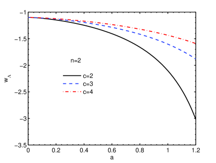
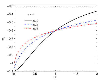
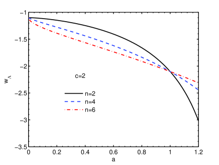
In Fig. (1), the evolution of as a function of scale
factor is plotted for different values of the parameters and
.The other interesting aspect of the polytropic gas is that the
interacting polytropic gas dark energy crosses the phantom divide
from to (see Fig.(1), left
panels). This behavior of polytropic gas is similar to interacting
agegraphic dark energy model in which the phantom divide is crossed
from below to up (see Figs.(2,3) of cai44 ). The similarity of
the interacting agegraphic dark energy and polytropic gas is that
both models cross the phantom divide from below to up. In upper
panels we fix the polytropic index as and in lower panels the
parameter is fixed. In upper left panel the negative values of
are selected to obtain the transition from phantom to
quintessence regime. In upper right panel, the positive values of
are selected. In this case the interacting polytropic gas
behaves as a phantom like field. Same as left panel, we fix the
polytropic index . Here, one can easily find the phantom
behavior of polytropic gas model. It is worth noting that the
phantom regime of polytropic gas model is restricted with a
characteristic scale factor , where we
encounter with a singularity at this epoch. In lower panels of
Fig.(1), the dependency of the evolution of on the
polytropic index parameter is studied. In lower left panel, by
fixing , we studied this dependency for polytropic gas model.
It is easy to see that the larger value of gets the larger
at and smaller at . In lower
right panel, by fixing , the dependency of on the
parameter is investigated for phantom polytropic gas model.
Unlike to lower left panel, the larger value of gets the smaller
at and larger at .
In order to obtain the evolution of dimensionless energy density, , let us start with Eqs.(9) and (3) and obtain the density parameter of interacting polytropic gas as
| (13) |
Taking the derivative of Eq.(13) with respect to time and using , we can obtain
| (14) |
where prime denotes the derivative with respect to . Taking the derivative of Friedmann equation (2) with respect to time and using Eqs.(9), (4), (6), (13) and , one can find that
| (15) |
Substituting this relation into Eq.(14), we obtain the evolutionary equation for energy density parameter of interacting polytropic gas as:
| (16) |
where is given by
| (17) |
and .
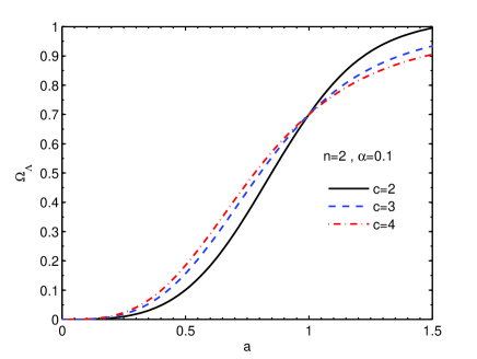
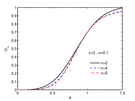
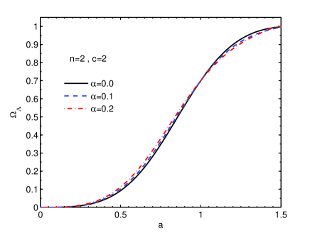
In Fig.(2), by solving the differential
equation (16), we show the evolution of
for different model parameters and as
well as different interaction parameter . Here we assume
only the positive values of , i.e., the phantom polytropic gas
model. The numerical values of density parameters at the present
time are taken as: , and
. In upper panels, we consider the non-interacting
polytropic gas and in lower panel the interaction term is included.
Here, we see that at the early time
and tends to at the late time. Hence the polytropic gas model
can describe the matter-dominated universe in the far past. Also, at
the late time, we encounter with dark energy dominated universe
(). In upper left panel, by fixing
the parameter , the polytropic gas starts to be effective earlier
and tends to a lower value at the late time when
is larger. On the other hand, in upper right panel, we see that
for fixed parameter , the polytropic gas starts to be effective
earlier and also tends to a higher value at the
late time when is smaller. In lower panel, the effect of
interaction parameter on the evolution of
is studied. Here one can see that the polytropic
gas starts to be effective earlier, by increasing the interaction
parameter . Also, at , the parameter
is smaller for
larger values of .
For completeness, we derive the deceleration parameter
| (18) |
for polytropic gas model. Substituting Eq.(15) in (18) we get
| (19) |
It is worth noting that in the limiting case of matter-dominated
phase and considering flat universe in the absence of interaction
term, Eq.(19) is reduced to which represents the
decelerated expansion () of the universe.
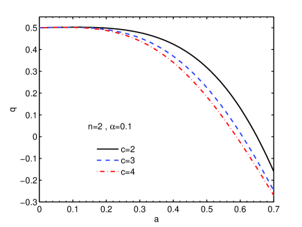
In Fig.(3), we show the evolution of as a function of for
different model parameters and as well as different
interaction parameter . Here we discuss the evolution of
for phantom polytropic gas model, by assuming positive . Upper
panels is plotted in the absence of interaction between dark energy
and dark matter
and the lower panel is plotted in the presence of interaction term.
The parameter converges to at the early time, whereas the universe
is dominated by pressureless dark matter. In upper left panel, by
fixing , the accelerated expansion is achieved earlier by
increasing . Also, in the upper right panel, we see that by
increasing , becomes larger at the deceleration phase and
gets smaller at the acceleration phase. It is worth noting that,
although, both the model parameters and impact the evolution
of deceleration parameter , but the change of sign from to
depends on the parameter of the model.
III Correspondence between polytropic gas DE model and scalar fields
In the present section we establish a correspondence between the interacting polytropic gas model with the tachyon, K-essence and dilaton scalar field models. The importance of this correspondence is that the scalar field models are an effective description of an underlying theory of dark energy and therefore it is worthwhile to reconstruct the potential and the dynamics of scalar fields according the evolutionary form of polytropic gas model. For this aim, first we compare the energy density of polytropic gas model (i.e. Eq.9) with the energy density of corresponding scalar field model. Then, we equate the equations of state of scalar field models with the EoS parameter of polytropic gas (i.e. Eq.12).
III.1 Polytropic gas tachyon model
It is believed that the tachyon can be assumed as a source of DE c24 . The tachyon is an unstable field which can be used in string theory through its role in the Dirac-Born-Infeld (DBI) action to describe the D-bran action c25 . The effective Lagrangian for the tachyon field is given by
where is the potential of tachyon. The energy density and pressure of tachyon field are c25
| (20) |
| (21) |
The EoS parameter of tachyon can be obtained as
| (22) |
In order to have a real energy density for tachyon field, it is required that . Consequently, from Eq.(22), the EoS parameter of tachyon is constrained to . Hence, the tachyon field can interpret the accelerates expansion of universe, but it can not enter the phantom regime, i.e. . In order to reconstruct the potential and the dynamics of tachyon according to evolution of interacting polytropic gas model, we should equate Eqs.(12) and (22) and also Eq.(9) with Eq.(20) as follows
| (23) |
| (24) |
Hence we get the following expressions for dynamics and potential of tachyon field
| (25) |
| (26) |
For , from Eq.(25), we obtain which represents the phantom behavior of tachyon field. It is worth noting that the reconstructed tachyon field according to the interacting polytropic gas can cross the phantom divide. By definition and changing the time derivative to the derivative with respect to logarithmic scale factor, i.e. , the scalar field can be integrated from Eq.(25) as follows
| (27) |
III.2 Polytropic gas K-essence model
The idea of the K-essence scalar field was motivated from the Born-Infeld action of string theory and can explain the late time acceleration of the universe c26 . The general scalar field action for K-essence model as a function of and is given by c27
| (28) |
where the Lagrangian density relates to a pressure density and energy density through the following equations:
| (29) |
| (30) |
Hence, the EoS parameter of K-essence scalar field is obtained as
| (31) |
By comparing Eqs.(12) and (31), we have
| (32) |
Hence the parameter is obtained as
| (33) |
From Eq.(31), one can see the phantom behavior of K-essence scalar field () when the parameter lies in the interval .
Using and changing the time derivative to the derivative with respect to , we obtain
| (34) |
The integration of Eq.(34) yields
| (35) |
Here, we reconstructed the potential and the dynamics of K-essence scalar field according to the evolutionary form of the interacting polytropic gas model. The K-essence polytropic gas model can explain the accelerating universe and also behaves as a phantom model provided .
III.3 Polytropic gas dilaton model
A dilaton scalar field can also be assumed as a source of DE. This scalar field is originated from the lower-energy limit of string theory c28 . The dilaton filed is described by the effective Lagrangian density as
| (36) |
where and are positive constant. Considering the dilaton field as a source of the energy-momentum tensor in Einstein equations, one can find that the Lagrangian density corresponds to the pressure of the scalar field and the energy density of dilaton field is also obtained as
| (37) |
Here . The negative coefficient of the kinematic term of the dilaton field in Einstein frame makes a phantom like behavior for dilaton field. The EoS parameter of dilaton is given by
| (38) |
In order to consider the dilaton field as a description of polytropic gas, we establish the correspondence between the dilaton EoS parameter,, and the EoS parameter of polytropic gas model. By equating Eq.(38) with Eq.(12), we find
| (39) |
By using and , the scalar field can be obtained as
| (40) |
Here we presented the reconstructed potential and dynamics of dilaton scalar field according to the evolution of interacting polytropic gas model.
IV Conclusion
In this work we presented the interacting polytropic gas model of
dark energy to interpret the accelerated expansion of the universe.
Assuming a non-flat FRW universe dominated by interacting polytropic
gas DE and CDM, we studied the cosmic behavior of polytropic gas
model. For this aim, we calculated the evolution of effective EoS
parameter and showed that for positive values
with even numbers of this model behaves as a phantom DE model
and in the case of it treats as a
quintessence model. Similar to interacting agegraphic dark energy
model, the interacting polytropic gas model crosses the phantom
divide from below () to up (). The
transition from phantom to quintessence depends on the parameter
of the model. For larger value of , the transition take place
sooner. In the case of phantom polytropic gas model,
is larger for larger value of . In the scenario of polytropic gas
model, the phantom divide can be crossed even in the absence of
interaction. We also calculated the evolution of energy density
. The matter dominated phase at the early time and
DE-dominated universe at the late time can be described in the
context of polytropic gas model. The polytropic gas starts to be
effective earlier for larger value of interaction parameter as well
as for larger value of the parameter or smaller value of . We
calculated the deceleration parameter and obtained the
decelerated and accelerated expansion phases of the universe in the
context of polytropic gas model. The transition from decelerated
expansion () to accelerated expansion () takes place
sooner for larger value of and also by increasing the
interaction parameter . Since the scalar fields models are
the underlying theory of dark energy, we proposed a correspondence
between interacting polytropic gas model with the tachyon, K-essence
and dilaton scalar fields models. We reconstructed the potential and
the dynamics of these scalar fields according to the evolution of
the interacting
polytropic gas model.
Acknowledgements.
This work has been supported by Research Institute for Astronomy and Astrophysics of Maragha, Iran.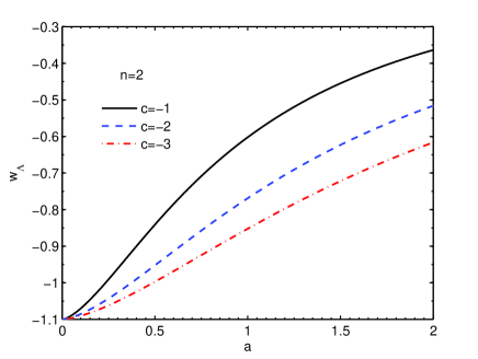
References
- (1) S. Perlmutter et al., Astrophys. J. 517, 565 (1999).
- (2) C. L. Bennett et al., Astrophys. J. Suppl. 148, 1 (2003).
- (3) M. Tegmark et al., Phys. Rev. D 69, 103501 (2004).
- (4) S. W. Allen, et al., Mon. Not. Roy. Astron. Soc. 353, 457 (2004).
- (5) U. Alam, V. Sahni and A. A. Starobinsky, JCAP 0406 (2004) 008; D. Huterer and A. Cooray, Phys. Rev. D 71 (2005) 023506; Y.G. Gong, Int. J. Mod. Phys. D 14 (2005) 599; Y.G. Gong, Class. Quantum Grav. 22 (2005) 2121; Yun Wang and M. Tegmark, Phys. Rev. D 71 (2005) 103513; Yun-gui Gong and Yuan-Zhong Zhang, Phys. Rev. D 72 (2005) 043518.
-
(6)
C. Wetterich, Nucl. Phys. B 302, 668 (1988);
B. Ratra, J. Peebles, Phys. Rev. D 37, 321 (1988). -
(7)
R. R. Caldwell, Phys. Lett. B 545, 23 (2002);
S. Nojiri, S.D. Odintsov, Phys. Lett. B 562, 147 (2003);
S. Nojiri, S.D. Odintsov, Phys. Lett. B 565, 1 (2003). -
(8)
E. Elizalde, S. Nojiri, S.D. Odinstov, Phys. Rev. D 70, 043539 (2004);
S. Nojiri, S.D. Odintsov, S. Tsujikawa, Phys. Rev. D 71, 063004 (2005);
A. Anisimov, E. Babichev, A. Vikman, J. Cosmol. Astropart. Phys. 06, 006 (2005). -
(9)
T. Chiba, T. Okabe, M. Yamaguchi, Phys. Rev. D 62,
023511(2000);
C. Armend ariz-Pic on, V. Mukhanov, P.J. Steinhardt, Phys. Rev. Lett. 85, 4438 (2000);
C. Armend ariz-Pic on, V. Mukhanov, P.J. Steinhardt, Phys. Rev. D 63, 103510 (2001). -
(10)
A. Sen, J. High Energy Phys. 04, 048 (2002);
T. Padmanabhan, Phys. Rev. D 66, 021301 (2002);
T. Padmanabhan, T.R. Choudhury, Phys. Rev. D 66, 081301 (2002). - (11) M. Gasperini, F. Piazza, G. Veneziano, Phys. Rev. D 65, 023508 (2002); N. Arkani-Hamed, P. Creminelli, S. Mukohyama, M. Zaldarriaga, J. Cosmol. Astropart. Phys. 04, 001 (2004); F. Piazza, S. Tsujikawa, J. Cosmol. Astropart. Phys. 07, 004 (2004).
- (12) A. Kamenshchik, U. Moschella, V. Pasquier, Phys. Lett. B 511, 265 (2001); M. C. Bento, O. Bertolami, A. A. Sen, Phys. Rev. D 66, 043507 (2002);
- (13) M. R. Setare, Eur. Phys. J. C 52, 689, 2007.
- (14) C. Deffayet, G. R. Dvali, G. Gabadaaze, Phys. Rev. D 65, 044023 (2002); V. Sahni, Y. Shtanov, J. Cosmol. Astropart. Phys. 0311, 014 (2003).
- (15) P. Horava, D. Minic, Phys. Rev. Lett. 85, 1610 (2000); P. Horava, D. Minic, Phys. Rev. Lett. 509, 138 (2001); S. Thomas, Phys. Rev. Lett. 89, 081301 (2002); M. R. Setare, Phys. Lett. B 644, 99, 2007; M. R. Setare, Phys. Lett. B 654, 1, 2007; M. R. Setare, Phys. Lett. B 642, 1, 2006; M. R. Setare, Eur. Phys. J. C 50, 991, 2007; M. R. Setare, Phys. Lett. B 648, 329, 2007; M. R. Setare, Phys. Lett. B 653, 116, 2007.
- (16) R.G. Cai, Phys. Lett. B 657, (2007) 228; H. Wei, R.G. Cai, Phys. Lett. B 660, 113 (2008).
- (17) G. t Hooft, gr-qc/9310026; L. Susskind, J. Math. Phys. 36, 6377 (1995).
- (18) F. Karolyhazy, Nuovo.Cim. A 42 (1966) 390; F. Karolyhazy, A. Frenkel and B. Lukacs, in Physics as natural Philosophy edited by A. Shimony and H. Feschbach, MIT Press, Cambridge, MA, (1982); F. Karolyhazy, A. Frenkel and B. Lukacs, in Quantum Concepts in Space and Time edited by R. Penrose and C.J. Isham, Clarendon Press, Oxford, (1986).
- (19) O. Bertolami, F. Gil Pedro, M. Le Delliou, Phys. Lett. B 654, 165 (2007).
- (20) C. Feng, B. Wang, Y. Gong, R.K. Su, JCAP 0709, 005 (2007).
- (21) C.L. Bennett et al., Astrophys. J. Suppl. 148, 1 (2003); D.N. Spergel, Astrophys. J. Suppl. 148, 175 (2003); M. Tegmark et al., Phys. Rev. D 69, 103501 (2004); U. Seljak, A. Slosar, P. McDonald, J. Cosmol. Astropart. Phys. 10, 014 (2006); D.N. Spergel et al., Astrophys. J. Suppl. 170, 377 (2007).
- (22) U. Mukhopadhyay and S. Ray, Mod. Phys. Lett. A 23, 3198,2008.
- (23) K. Karami, A. Abdolmaleki, Astrophys. Space Sci.330, 133,2010.
- (24) K. Karami, S. Ghaffari, J. Fehri, Eur. Phys. J. C, 64, 85 (2009).
- (25) S. Nojiri, S. D. Odintsov, S. Tsujikawa, Phys. Rev. D 71, 063004 (2005).
- (26) H. Wei, R. G. Cai, Eur.Phys.J.C59, 105, 2009.
- (27) K. Karami, A. Abdolmaleki, arXiv:1009.3587.
- (28) J. Christensen-Dalsgard, Lecture Notes on Stellar Structure and Evolution, 6th edn. (Aarhus University Press, Aarhus, 2004).
- (29) D. N. Spergel, et al., Satrophys. J. Suppl. 170, 377 (2007).
- (30) A. Sheykhi, Phys. Lett. B 680, 113 (2009); H. Wei & R. G. Cai, Phys. Lett. B 660, 113 (2008); L. Zhang, J. Cui, J. Zhang & X. Zhang, Int. J. Mod. Phys. D 19, 21 (2010).
- (31) L. P. Chimento, Phys. Rev. D 81, 043525 (2010).
-
(32)
L. Amendola, Phys. Rev. D 60 (1999) 043501;
L. Amendola, Phys. Rev. D 62 (2000) 043511;
L. Amendola and C. Quercellini, Phys. Rev. D 68 (2003) 023514;
L. Amendola and D. Tocchini-Valentini, Phys. Rev. D 64 (2001) 043509 ;
L. Amendola and D. T. Valentini, Phys. Rev. D 66 (2002) 043528. - (33) J. S. Bagla, H. K. Jassal, T. Padmanabhan, Phys. Rev. D 67, 063504 (2003), astro-ph/0212198 Ying Shao, Yuan-Xing Gui and Wei Wang, Mod. Phys. Lett. A 22, 1175-1182 (2007), gr-qc/0703112 Gianluca Calcagni and Andrew R. Liddle, Phys. Rev. D 74, 043528,2006, astro-ph/0606003 Edmund J. Copeland, Mohammad R. Garousi, M. Sami and Shinji Tsujikawa, Phys. Rev. D 71, 043003 (2005), hep-th/0411192
- (34) A. Sen, JHEP 0204, 048 (2002); JHEP 0207, 065 (2002); Mod. Phys. Lett. A 17, 1797 (2002); arXiv: hep- th/0312153;A. Sen, JHEP 9910, 008 (1999); E. A. Bergshoeff, M. de Roo, T. C. de Wit, E. Eyras, S. Panda, JHEP 0005, 009 (2000); J. Kluson, Phys. Rev. D 62, 126003 (2000); D. Kutasov and V. Niarchos, Nucl. Phys. B 666, 56, (2003).
- (35) A. Sen, Mod. Phys. Lett. A 17 (2002) 1797; N. D. Lambert, I. Sachs, Phys. Rev. D 67 (2003) 026005.
- (36) T. Chiba et al., Phys. Rev. D 62 (2000) 023511; C. Armendariz-Picon et al., Phys. Rev. Lett 85 (2000) 4438; C. Armendariz-Picon et al., Phys. Rev. Lett 63 (2001) 103510.
- (37) F. Piazza and S. Tsujikawa, JCAP 0407, 004 (2004).