Charm baryon spectroscopy at CDF

Abstract:

Due to an excellent mass resolution and a large amount of available data, the CDF experiment, located at the Tevatron proton-antiproton accelerator, allows the precise measurement of spectroscopic properties, like mass and decay width, of a variety of states. This was exploited to examine the first orbital excitations of the $\Lambda_{c}$ baryon, the resonances $\Lambda_{c}(2595)$ and $\Lambda_{c}(2625)$, in the decay channel $\Lambda_{c}^{+}\,\pi^{+}\,\pi^{-}$, as well as the $\Lambda_{c}$ spin excitations $\Sigma_{c}(2455)$ and $\Sigma_{c}(2520)$ in its decays to $\Lambda_{c}^{+}\,\pi^{-}$ and $\Lambda_{c}^{+}\,\pi^{+}$ final states in a data sample corresponding to an integrated luminosity of $5.2\,\mathrm{fb}^{-1}$. We present measurements of the mass differences with respect to the $\Lambda_{c}$ and the decay widths of these states, using significantly higher statistics than previous experiments.

1 Introduction

Heavy quark baryons provide an interesting laboratory for studying and testing Quantum Chromodynamics (QCD), the theory of strong interactions. The heavy quark states test regions of the QCD where perturbation calculations cannot be used, and many different approaches to solve the theory were developed. In this write-up we focus on $\Lambda_{c}(2595)$, $\Lambda_{c}(2625)$, $\Sigma_{c}(2455)$ and $\Sigma_{c}(2520)$ baryons. All four states were observed before and some of their properties measured [1]. However, different mass measurements for $\Sigma_{c}(2520)$ and $\Lambda_{c}(2625)$ are inconsistent and the statistics for $\Lambda_{c}(2595)$ and $\Lambda_{c}(2625)$ is rather low. In addition, Blechman and co-workers showed that a more sophisticated treatment, which would take into account the proximity of the threshold in the $\Lambda_{c}(2595)$ decay, yields a $\Lambda_{c}(2595)$ mass which is $2-3\,\mathrm{MeV}/c^{2}$ lower than the one observed [2]. $\Sigma_{c}$ states were observed and studied in $\Lambda_{c}\pi$ decays, while excited $\Lambda_{c}$ states decay mainly to a $\Lambda_{c}\pi\pi$ final state and decays through intermediated $\Sigma_{c}$ resonances are possible. One peculiarity of the experimental studies of these baryons is in their cross talks, which requires special care in the treatment of the background due to different kinematic regions allowed for different sources.

In this analysis we exploit a large sample of $\Lambda_{c}^{+}\rightarrow pK^{-}\pi^{+}$ decays collected by the CDF detector to perform the measurement of the masses and widths of the discussed charmed baryons. We take into account all cross-talks and threshold effects expected in the decays under study [3]. Throughout this document the use of a specific particle state implies the use of the charge-conjugate state as well.

2 Analysis Strategy

The employed dataset corresponds to an integrated luminosity of $5.2\,\mathrm{fb^{-1}}$ and was collected using the displaced track trigger which requires two charged particles coming from a single vertex with transverse momenta larger than $2\,\mathrm{GeV}/c$ and impact parameters in the plane transverse to the beamline in the region of $0.1$ to $1\,\mathrm{mm}$.

The selection of the candidates is done in two steps. As all final states feature a $\Lambda_{c}$ daughter, as first step we perform a $\Lambda_{c}$ selection. In the second step we perform a dedicated selection of the four states under study. In each step we use neural networks to distinguish signal from background. All neural networks [4] are trained using data only by means of the ${}_{s}\mathcal{P}lot$ technique [5]. As we use only data for the neural network trainings, for each case we split the sample to two parts (even and odd event numbers) and train two networks. Each of them is applied to the complementary subsample in order to maintain a selection which is trained on a sample independent from the one to which we apply it.

In order to determine the mass differences relative to the $\Lambda_{c}$ and the decay widths of the six studied states, we perform binned maximum likelihood fits of three separate mass difference ($\Delta M$) distributions. The first two are $\Lambda_{c}^{+}\pi^{+}$ and $\Lambda_{c}^{+}\pi^{-}$ where the states $\Sigma_{c}(2455)^{++,0}$ and $\Sigma_{c}(2520)^{++,0}$ are studied. The last one is $\Lambda_{c}^{+}\pi^{+}\pi^{-}$ for $\Lambda_{c}(2595)^{+}$ and $\Lambda_{c}(2625)^{+}$. In each of the distributions we need to parametrize two signals and several background components.

Both $\Sigma_{c}(2455)^{++,0}$ and $\Sigma_{c}(2520)^{++,0}$ are described by a nonrelativistic Breit-Wigner function convolved with a resolution function. The resolution function is parametrized with three Gaussians centered in zero and other parameters derived from simulated events. The mean width of the resolution function is about $1.6\,\mathrm{MeV}/c^{2}$ for $\Sigma_{c}(2455)^{++,0}$ and about $2.6\,\mathrm{MeV}/c^{2}$ for $\Sigma_{c}(2520)^{++,0}$. We consider three different types of background, namely random combinations without real $\Lambda_{c}$, combinations of real $\Lambda_{c}$ with a random pion and events due to the decay of excited $\Lambda_{c}$ to $\Lambda_{c}^{+}\pi^{+}\pi^{-}$. Thereby, random combinations without a real $\Lambda_{c}$ dominate and are described by a second-order polynomial with shape and normalization derived in a fit to the $\Delta M$ distribution from $\Lambda_{c}$ mass sidebands. The apparent difference between doubly-charged and neutral combinations is due to $D^{*}(2010)^{+}$ mesons with multibody $D^{0}$ decays, where not all $D^{0}$ decay products are reconstructed. In order to describe this reflection, an additional Gaussian function is used. The second background source, consisting of real $\Lambda_{c}$ combined with a random pion, is modeled by a third-order polynomial. As we do not have an independent proxy for this source, all parameters are left free in the fit. The last source, originating from nonresonant $\Lambda_{c}(2625)$ decays, is described by the projections of the flat $\Lambda_{c}^{+}\pi^{+}\pi^{-}$ Dalitz plot on the appropriate $\Lambda_{c}^{+}\pi^{+}$ respective $\Lambda_{c}^{+}\pi^{-}$ axes. The measured data distributions together with the fit projections can be found in figure 1.

a)               b)

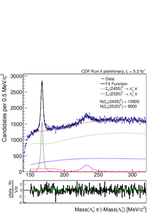
Figure 1: The (a) $M(\Lambda_{c}^{+}\pi^{+})-M(\Lambda_{c}^{+})$ and (b) $M(\Lambda_{c}^{+}\pi^{-})-M(\Lambda_{c}^{+})$ distribution obtained from data (points with error bars) together with the fit projection (black line). The brown and purple lines correspond to the two signal contributions, the green line represents the combinatorial background without real $\Lambda_{c}$, the blue line shows real $\Lambda_{c}$ combined with a random pion and the red dotted line represents a reflection from excited $\Lambda_{c}$ decays. The red dashed line corresponds to the sum of all three background contributions.

In the fit for $\Lambda_{c}(2595)$ and $\Lambda_{c}(2625)$, an additional complication compared to the $\Sigma_{c}$ case arises from the fact that previous measurements of the $\Lambda_{c}(2595)$ properties indicate that it decays dominantly to $\Sigma_{c}(2455)\pi$, which has its threshold very close to the $\Lambda_{c}(2595)$ mass. Ref. [2] shows that taking into account the resulting strong variation of the natural width yields a lower $\Lambda_{c}(2595)$ mass than observed by former experiments. With CDF statistics we are much more sensitive to the details of the $\Lambda_{c}(2595)$ line shape than previous analyses. The $\Lambda_{c}(2595)$ parametrization follows Ref. [2]. The state is described by a nonrelativistic Breit-Wigner function with a mass-dependent decay width which is calculated as integral over the Dalitz plot containing the $\Sigma_{c}(2455)$ resonances. The pion coupling constant $h_{2}$ is related to the $\Lambda_{c}(2595)$ decay width and represents the quantity we measure instead of the natural width. The shape is then numerically convolved with a three Gaussian resolution function determined from simulation, which has a mean width of about $1.8\,\mathrm{MeV}/c^{2}$. The signal function for the $\Lambda_{c}(2625)$ is a nonrelativistic Breit-Wigner which is again convolved with a three Gaussian resolution function determined from simulation. The mean width of the resolution function is about $2.4\,\mathrm{MeV}/c^{2}$. The background consists of three different sources which are combinatorial background without real $\Lambda_{c}$, real $\Lambda_{c}$ combined with two random pions and real $\Sigma_{c}^{++,0}$ combined with a random pion. The combinatorial background without real $\Lambda_{c}$ is parametrized by a second order polynomial whose parameters are determined in a fit to the $\Delta M$ distribution of candidates from $\Lambda_{c}$ mass sidebands. The second source, consisting of real $\Lambda_{c}$ combined with two random pions, is parametrized by a second order polynomial with all parameters allowed to float in the fit. The model of the final background source, real $\Sigma_{c}(2455)$ combined with a random pion, is based on a uniform function defined from the threshold to the end of the fit range, where the natural widths as well as the resolution effects of the $\Sigma_{c}(2455)^{++,0}$ are taken into account for the threshold determination. The size of this contribution is constrained to the $\Sigma_{c}(2455)$ yield obtained from fits to the projections of the $\Lambda_{c}^{+}\pi^{+}\pi^{-}$ Dalitz plot from the upper $\Lambda_{c}(2625)$ mass sideband on the appropriate $\Lambda_{c}^{+}\pi^{+}$ respective $\Lambda_{c}^{+}\pi^{-}$ axes. The measured data distribution together with the fit projection can be found in figure 2.

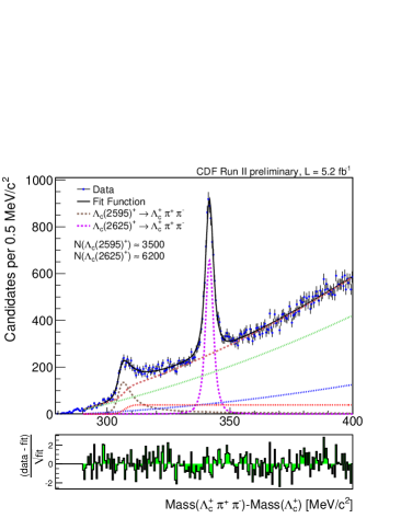
Figure 2: The $M(\Lambda_{c}^{+}\pi^{+}\pi^{-})-M(\Lambda_{c}^{+})$ distribution obtained from data (points with error bars) together with the fit projection (black line). The brown and purple lines correspond to the two signal contributions, the green line represents the combinatorial background without real $\Lambda_{c}$, the blue line shows real $\Lambda_{c}$ combined with two random pions and the red dotted line represents real $\Sigma_{c}(2455)$ combined with a random pion. The red dashed line corresponds to the sum of all three background contributions.

We investigate several systematic effects which can affect our measurements. Generally, they can be categorized as imperfect modeling by the simulation, imperfect knowledge of the momentum scale of the detector, ambiguities in the fit model and uncertainties on the external inputs to the fit of the $\Lambda_{c}(2595)$ signal. The most critical point is that we need to understand the intrinsic resolution of the detector in order to properly describe the signal shapes, because an uncertainty in the resolution has a large impact on the determination of the natural widths. As we estimate it using simulated events, it is necessary to substantiate that the resolution obtained from simulation agrees with the one in real data. We use $D^{*}(2010)^{+}\rightarrow D^{0}\pi^{+}$ with $D^{0}\rightarrow K^{-}\pi^{+}$ and $\psi(2S)\rightarrow J/\psi\pi^{+}\pi^{-}$ with $J/\psi\rightarrow\mu^{+}\mu^{-}$ for this purpose and compare the resolution in data and simulated events as a function of the transverse momentum of the pions added to $D^{0}$ or $J/\psi$. We also compare the overall resolution scale between data and simulated events and find that all variations are below 20% which we assign as uncertainty on our knowledge of the resolution function.

3 Results

We select about 13800 $\Sigma_{c}(2455)^{++}$, 15900 $\Sigma_{c}(2455)^{0}$, 8800 $\Sigma_{c}(2520)^{++}$, 9000 $\Sigma_{c}(2520)^{0}$, 3500 $\Lambda_{c}(2595)^{+}$ and 6200 $\Lambda_{c}(2625)^{+}$ signal events and obtain the following results for the mass differences relative to the $\Lambda_{c}$ mass and the decay widths:

$$\Delta M(\Sigma_{c}(2455)^{++}) = 167.44\pm 0.04\,\mathrm{(stat.)}\pm 0.12\,\mathrm{(syst.)}\,\mathrm{MeV}/c^{2},$$

$$\Gamma(\Sigma_{c}(2455)^{++}) = 2.34\pm 0.13\,\mathrm{(stat.)}\pm 0.45\,\mathrm{(syst.)}\,\mathrm{MeV}/c^{2},$$

$$\Delta M(\Sigma_{c}(2455)^{0}) = 167.28\pm 0.03\,\mathrm{(stat.)}\pm 0.12\,\mathrm{(syst.)}\,\mathrm{MeV}/c^{2},$$

$$\Gamma(\Sigma_{c}(2455)^{0}) = 1.65\pm 0.11\,\mathrm{(stat.)}\pm 0.49\,\mathrm{(syst.)}\,\mathrm{MeV}/c^{2},$$

$$\Delta M(\Sigma_{c}(2520)^{++}) = 230.73\pm 0.56\,\mathrm{(stat.)}\pm 0.16\,\mathrm{(syst.)}\,\mathrm{MeV}/c^{2},$$

$$\Gamma(\Sigma_{c}(2520)^{++}) = 15.03\pm 2.12\,\mathrm{(stat.)}\pm 1.36\,\mathrm{(syst.)}\,\mathrm{MeV}/c^{2},$$

$$\Delta M(\Sigma_{c}(2520)^{0}) = 232.88\pm 0.43\,\mathrm{(stat.)}\pm 0.16\,\mathrm{(syst.)}\,\mathrm{MeV}/c^{2},$$

$$\Gamma(\Sigma_{c}(2520)^{0}) = 12.51\pm 1.82\,\mathrm{(stat.)}\pm 1.37\,\mathrm{(syst.)}\,\mathrm{MeV}/c^{2},$$

$$\Delta M(\Lambda_{c}(2595)^{+}) = 305.79\pm 0.14\,\mathrm{(stat.)}\pm 0.20\,\mathrm{(syst.)}\,\mathrm{MeV}/c^{2},$$

$$h_{2}^{2}(\Lambda_{c}(2595)^{+}) = 0.36\pm 0.04\,\mathrm{(stat.)}\pm 0.07\,\mathrm{(syst.)},$$

$$\Delta M(\Lambda_{c}(2625)^{+}) = 341.65\pm 0.04\,\mathrm{(stat.)}\pm 0.12\,\mathrm{(syst.)}\,\mathrm{MeV}/c^{2}.$$

For the width of the $\Lambda_{c}(2625)$ we get a value consistent with zero and therefore calculate an upper limit using a Bayesian approach with a uniform prior restricted to positive values. At the 90% C.L. we obtain $\Gamma(\Lambda_{c}(2625)^{+})<0.97\,\mathrm{MeV}/c^{2}$. For easier comparison to previous results, $h_{2}^{2}$ corresponds to $\Gamma(\Lambda_{c}(2595)^{+})=2.59\pm 0.30\pm 0.47\,\mathrm{MeV}/c^{2}$.

Except of $\Delta M(\Lambda_{c}(2595)^{+})$, all measured quantities are in agreement with previous measurements. For $\Delta M(\Lambda_{c}(2595)^{+})$ we observe a value which is by $3.1\,\mathrm{MeV}/c^{2}$ smaller than the existing world average. This difference is of the same size as found in Ref. [2]. The precision for the $\Sigma_{c}$ states is comparable to the precision of the world averages. In the case of excited $\Lambda_{c}$ states, our results provide a significant improvement in precision against previous measurements.

References

- [1] C. Amsler et al. (Particle Data Group), Review of Particle Physics, Phys. Lett. B667, 1 (2008).
- [2] A. Blechman, A. Falk and D. Pirjol, Threshold effects in excited charmed baryon decays, Phys. Rev. D67, 074033 (2003).
-
[3]
CDF Public Note 10260: http://www-cdf.fnal.gov/physics/new/bottom/100701.blessed-Charm_Baryons/
cdf10260_CharmBaryons.pdf - [4] M. Feindt and U. Kerzel, The NeuroBayes neural network package, Nucl. Instrum. Meth. A559, 190-194 (2006).
- [5] M. Pivk and F. Le Diberder, sPlot: a statistical tool to unfold data distributions, Nucl. Instrum. Meth. A555, 356-369 (2005).