On the determination of cusp points of 3-RPR parallel manipulators
Abstract
This paper investigates the cuspidal configurations of 3-RPR parallel manipulators that may appear on their singular surfaces in the joint space. Cusp points play an important role in the kinematic behavior of parallel manipulators since they make possible a non-singular change of assembly mode. In previous works, the cusp points were calculated in sections of the joint space by solving a 24th-degree polynomial without any proof that this polynomial was the only one that gives all solutions. The purpose of this study is to propose a rigorous methodology to determine the cusp points of 3-RPR manipulators and to certify that all cusp points are found. This methodology uses the notion of discriminant varieties and resorts to Gröbner bases for the solutions of systems of equations.
KEY WORDS : Kinematics, Singularities, Cusp, Parallel manipulator, Symbolic computation
1 Introduction
Because at a singularity a parallel manipulator loses its stiffness, it is of primary importance to be able to characterize these special configurations. This is, however, a very challenging task for a general parallel manipulator. Planar parallel manipulators have received a lot of attention [1-5] because of their relative simplicity with respect to their spatial counterparts. Moreover, studying the former may help understand the latter. Planar manipulators with three extensible leg-rods, referred to as 3-RPR manipulators, have often been studied. Such manipulators may have up to six assembly modes and their direct kinematics can be written in a polynomial of degree six [1, 2]. Moreover, they may have singularities (configurations where two direct kinematic solutions coincide). It was first pointed out that to move from one assembly mode to another, the manipulator should cross a singularity [3, 4]. Later, Innocenti and Parenti-Castelli [5] showed, using numerical experiments, that this statement is not true in general. In fact, this statement is only true under some special geometric conditions, such as similar base and mobile platforms [6, 7]. More recently, Macho et al. [8] proposed a method to plan non-singular assembly-mode changing trajectories. McAree [6] pointed out that for a 3-RPR parallel manipulator, if a point with triple direct kinematic solutions exists in the joint space, then the nonsingular change of assembly mode is possible. This result holds under some assumptions on the topology of the singularities [9]. For other mechanisms than 3-RPR manipulator, it is also interesting to note that encircling a cusp point is not the only way to execute a non-singular change of assembly mode [10]. A condition for three direct kinematic solutions to coincide was established in [6]. This condition was then exploited in [11] to derive a univariate polynomial of degree 96. A factored expression was obtained, one of the factors being a 24th-degree polynomial. The authors observed on many examples that the cusp points were each time defined by the 24th-degree polynomial, the remaining factors always defining spurious solutions only. However, they did not attempt to certify that the 24th-degree polynomial was really the only valid factor. Moreover, they never found more than 8 cusp points.
The purpose of this paper is to propose a rigorous methodology to determine the cusp points of any 3-RPR manipulator and to certify that all cusp points are found. This methodology uses the notion of discriminant varieties and resorts to Gröbner bases to solve the systems of equations. Using symbolic computation, it is verified that the cusp points are really defined by a 24th-degree polynomial. For any given 3-RPR manipulator geometry, the maximum number of cusp points in sectional sections of the joint space is determined and the results are certified. In particular, a robot with 10 cusp points in a cross section of its joint space is found for the first time.
The following section introduces the manipulators studied and recalls the main known results. Section 3 describes the algebraic tools used. Last section presents the methodology that is proposed to determine the cusp points using the algebraic tools.
2 Modeling and state of the art
2.1 Robot studied and Modeling
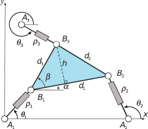
A general 3-RPR planar parallel manipulator is shown in Figure 1. This manipulator has three extensible leg-rods actuated with prismatic joints. This manipulator can move its moving platform in the plane. The vector of the three leg-rod lengths is (Figure 1). The geometric parameters of the manipulators are the three sides of the moving platform , , and the position of the base revolute joint centers , and . The reference frame is centered at and the x-axis passes through . Thus, , and .
| Parameters | Position variables | Equation constraints | |
|---|---|---|---|
| MD | |||
| GRS |
The position of the moving platform can be expressed by two different sets of variables (see also Table 1):
-
•
MD Model (McAree-Daniel): the 3 angles .
-
•
GSR Model (Gosselin-Sefriou-Richard): the position coordinates of point () and the platform orientation , ().
Each of these sets of variables leads to a different modeling system.
2.1.1 MD Model
The first model was used by MacAree and Daniel in [6] and has been extensively studied in [11]. Let define the three angles between the leg-rods and the x-axis. The six parameters (, ) define a configuration of the manipulator but only three of them are independent, so that the configuration space is a 3-dimensional manifold embedded in a 6-dimensional space. The dependency between (, ) is obtained by writing the constraint equations of the manipulator, namely, the fixed distances between the three vertices of the mobile platform :
| (1) |
where is the vector defining the coordinates of in the reference frame as function of and .
2.1.2 GSR Model
The GRS model was introduced in [12]. This model, combined with appropriate algebraic methods (see Section 3), will allow us to use a full symbolic computation of all cuspidal configurations. In this modeling, point and angle are used to specify the pose and the orientation of the platform. Let , where (resp. ) denotes (resp. ). Let (resp. ) denote (resp. ). With these variables, we can parametrize the positions of the three points and as follows:
The lengths define the geometric constraints of the robot, and can be written as the euclidian norm of the vectors . Finally, the dependency between can be identified by writing the distances between the vertices of the moving platform and the vertices of the base platform. These distances are the norms of the vectors :
| (2) |
where is the vector defining the constant coordinates of in the reference frame.
The formulas in Equations 2 can be expanded as follows:
| (3) |
The last polynomial in comes from the variable replaced by the variables and the equation constraint . This change of variables allows us to avoid the sine and cosine functions and keep the system algebraic. Moreover, this change of variables does not introduce any spurious solutions since the function
is bijective on the circle .
The following subsections recall the main properties of the 3-RPR manipulator observed using the MD Model.
2.2 Properties observed
In a special configuration (, ), the manipulator meets a singularity, where two assembly modes coalesce. This happens when the constraint Jacobian drops rank. A 3-RPR parallel manipulator is in a singularity whenever the three lines , are concurrent or parallel [13].
When three assembly modes coalesce, the manipulator is said to be in a cuspidal configuration. Using series expansion, McAree and Daniel show that in such configurations, the manipulator loses first and second order constraints. This gives a necessary condition for a manipulator to be in a cuspidal configuration (see Table 4).
Based on series expansion, [11] provided an algorithm to plot the singular curves in sectional slices of the joint space and to calculate the cusp points that appear on these curves. They calculated the cusp points in various sectional slices of the joint space for the manipulator defined by the following geometric parameters:
| (4) |
The following facts were observed in [11]:
-
•
no more than 8 cusp points were found in a sectional slice defined for a given value of ; this result was also observed in many other manipulator examples;
-
•
the number of cusp points per section stabilizes to four when exceeds a certain value;
-
•
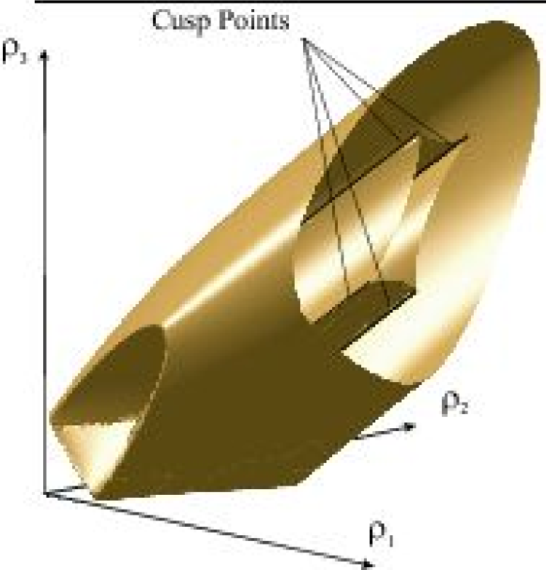
the set of all cusps points defined a set of curves in the 3-dimensional joint space (Fig. 2).
2.3 Limitations of the previous study
In [11], the cusp points were calculated in any sectional slice of the joint space by resorting to complex algebraic calculus based on expansion and elimination procedures. A univariate polynomial of degree 96 was obtained, which was shown to factor into several polynomials, one of which is of degree 24 and was conjectured to be the one that gives all cusp points in the sectional slice at hand. The other factors were found to give always spurious solutions. The following remarks can be drawn:
-
•
there is no proof that the above mentioned 24-degree polynomial is indeed the only polynomial that gives all solutions;
-
•
the sectional slices were analyzed by a discrete method, and, thus, the analysis was not exhaustive;
-
•
a maximum number of 8 cusps points were found in many manipulator examples, but there is no proof that no more than 8 solutions can be obtained.
-
•
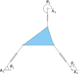
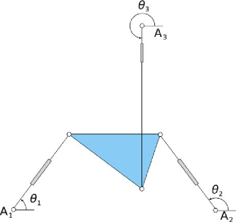
previous equation modeling does not distinguish between a platform triangle and its mirror image (see Figure 3), i.e. a triangle with the same but with an angle of opposite sign.
One limitation of the previous studies came from the algebraic tools used to describe the robot, which introduced spurious components that had to be removed with empirical observations. In the literature, another method exists based on the elimination of variables, reducing the problem to the computation of the triple roots of an univariate polynomial [14, 15, 2]. Unfortunately, due to the size of the univariate polynomial, this method ran out of memory when applied to 3-RPR manipulators [11].
(a) , , , , , , , ,
(b) , , , , , , , ,
The following section presents the minimal Discriminant Variety and the Jacobian criterion. These algebraic tools allowed us to compute and describe exactly the cuspidal configurations of the 3-RPR manipulators, without introducing any spurious components.
3 Algebraic tools
This section recalls some mathematic definitions and their implementation in Maple software. The parametric systems we consider are supposed to have a finite number of complex solutions for almost all parameter values. This property is checked by computing a Gröbner basis of the system at hand (see [16, page 274] and [17, Theorem 2] for more details).
3.1 Discriminant Variety
A Discriminant Variety [17] is associated to a parametric polynomial system . One of its main properties is that the real roots of can be parametrized continuously on each open connected set in the complement of .
Notations 1
In this section, we denote by a polynomial system of the form:
depending on the parameters and the variables .
For more simplicity, will be omitted in the subsequent sections.
For example, if we want to describe the number of solutions to the direct kinematics problem according to the articular parameters, then:
- •
-
•
the polynomial inequations are
-
•
the parameters are the articular variables and the variables are the pose variables .
The following definition is adapted from [17] for our problem.
Definition 1
(Discriminant Variety)
Let be any parametric system. With the notation defined above, we call Discriminant Variety of a set of parameter values such that on each connected part of :
-
i.
the roots of can be parametrized as continuous functions of the parameters;
-
ii.
the roots of do not cross.
Moreover, the intersection of all the discriminant varieties is called the minimal discriminant variety and is denoted by .
Remark 1
The conditions i. and ii. imply that for every open set in the complement of , the number of solutions is constant.
One of the main property of the minimal discriminant variety is that if has finitely solutions for almost all parameter values, then for each connected cell of , the number of solutions of restricted to is constant.
In the problem at hand, the minimal discriminant variety may be split into two components:
-
-
the inequation bounds in the parameters space. As far as a 3-RPR manipulator is considered, these bounds are trivial since the inequations already depend solely on the parameters;
-
-
the projection of the parallel singularities (defined in [18], see also section 3.3). These values are computed as follows:
-
1.
Compute as the minors of the Jacobian matrix:
-
2.
Eliminate the variables in the system
The zero iso-surface of the returned polynomials is the projection of the desired singularities.
-
1.
3.2 Degree of a -dimensional system and multiplicity of a root
The interested reader may find more detailed definitions on the degree and multiplicity in [19] or in [20, chapter 4].
Definition 2
(degree) Given a system of polynomial equations with finitely many complex solutions, the degree of is exactly the number of roots counted with multiplicities.
The following unusual definition is exactly the same as the classical one [20] (dimension of a local ring), the reader will find the correspondence in [21].
Definition 3
(multiplicity) Let be a system of polynomial equations in with finitely many complex solutions. Let be a linear form and a univariate polynomial returned by the computation of a rational univariate representation [21].
Then can be written as:
We call multiplicity of the exponent .
Remark 2
When is reduced to a univariate polynomial equation in X with roots
then the multiplicity of each root is exactly .
By extension, we can also define the multiplicity of the roots of a parametric system.
Definition 4
(multiplicity in a parametric system) Let be a parametric system depending on the parameters and on the variables . Assume furthermore that for all parameter values , the number of complex roots of is finite.
Then, the multiplicity of a root is the multiplicity of the root in the system .
Remark 3
This multiplicity definition can be naturally extended to define the multiplicity of a leaf above a connected component in the complement of the discriminant variety.
3.3 Jacobian criterion
We recall here the Jacobian criterion, used in this article to extract the points of multiplicity greater than or equal to . More details can be found in [22]. The Jacobian matrix to be considered here is exactly the same as the one used in [18] to define the singularities of type 2 of a manipulator. In this article, we will refer to these type-2 singularities as parallel singularities.
Theorem 1
Let be parametric polynomials of admitting a finite set of common complex roots for each value of the parameters . Let be the Jacobian matrix related to the variables :
If denotes the minors of , then for all , the following parametric system:
has a solution in if and only if the system
has at least one root of multiplicity greater than or equal to .
3.4 Software implementation in Maple
The algebraic tools used in this paper were adapted from the SALSA library developed at INRIA. The manipulations and computations of the algebraic objects are performed with the math software maple. The functions used are described below.
FGb
Given a set of polynomials generating an ideal , fgbrs:-fgb_gbasis allows the computation of a system of generators of the ideal. These generators provide a way to reduce any polynomial to a canonical unique form modulo . With the option ‘‘elim’’=true, it makes it possible to compute an algebraic system, the zero of which is the closure of the projection of the roots of .
This elimination of variables is based on Gröbner basis computations, using the algorithms F4 ([23]). As explained in the following sections, this function is used to compute the singular and cuspidal positions, as well as the discriminant variety.
RS
A system of polynomial equations is said -dimensional if its number of complex solutions is finite (this can be straightforwardly tested on a Gröbner basis of the system).
In this case, the RootFinding:-Isolate function computes directly the real solutions of . By default, each solution is given by a box with rational bounds, ensuring that no pairs of boxes overlaps. The algorithms implemented in Maple are based on the Rational Univariate Representation ([21]).
This function allows us to compute the number of cuspidal positions.
Discriminant Variety
Given a parametric system of equations and inequations , being the parameters and the unknowns, its minimal discriminant variety is computed with the algorithm presented in [17].
As shown further in section 4.3, the discriminant variety is a key tool for the description of the cuspidal positions.
This function is part of the package RootFinding[Parametric] in maple.
Limitations
These functions stand only for polynomials with rational coefficients. In particular, the trigonometric functions have to be replaced by algebraic variables.
4 New modelling and method
In this section and the subsequent ones, we use the equation system and the notations induced by the GSR Model presented in section 2.1.2. In this model, the position of the platform is given by variables: the coordinates of the point and , the cosine and sine of the angle respectively.
The configurations of a 3-RPR manipulator may be classified into three categories: the regular configurations, the singular configurations and the cuspidal configurations. The description of the special configurations (singular and cuspidal) is important for path planning. First, the regular configurations are the most common ones: these are the configurations where the position of the platform is locally uniquely determined by the values of the control parameters. Then the singular (resp. cuspidal) configurations are two (resp. three) coalesced configurations. These configurations were studied through local analysis in the past, but they can be also described with algebraic methods, as shown further in this article.
4.1 Singular configurations
From a geometrical point of view, we saw in Section 2.2 that a singular configuration represents coalesced assembly modes.
From an algebraic point of view, this condition can be retrieved in term of multiplicities. When the variables is specialized with real numbers, the set of equations (3) has finitely many solutions. Moreover, a multiplicity is associated with each solution (see Section 3.2). Using this notion, it can be verified that the singular assembly modes are exactly configurations that are solutions of multiplicity greater than or equal to . Indeed, the Jacobian criterion [22] states directly that these configurations are parallel singularities.
4.1.1 Modelling
To describe the singular points, we use the notion of multiplicity in a -dimensional system. The system of equations (3) is -dimensional when the lengths are given: it has a finite number of complex solutions. In this case, each solution can be associated with an integer greater than or equal to : its multiplicity, as defined in section 3.2.
Definition 5
A configuration of the 3-RPR manipulator is said singular if and only if is a solution of multiplicity greater than or equal to of:
To find the singular configurations, we use the Jacobian criterion, reminded in section 3.
Applying the Jacobian criterion [22] on the polynomial system Equations (3), we deduce that the singular configurations are exactly the solutions of the system:
| (5) |
Remark 4
By adding the determinant of the Jacobian matrix to Equations (3), we get a new system whose solutions are included in the original system. More precisely, the roots of Equations (5) are exactly the roots of multiplicity greater or equal to of Equations (3). The solutions to Equations (3) of multiplicity are solutions of multiplicity to Equations (5), and the solutions of multiplicity greater or equal to in Equations (3) have a multiplicity greater or equal to in Equations (5).
Moreover, using Gröbner basis computations to eliminate variables with Maple , a polynomial in the parametric variables , denoted , can be computed. Its solutions are exactly the sets of length values for which the manipulator admits singular configurations.
4.1.2 Example
In this section, the computation results are given for the manipulator example presented in [5, 6, 11, 24].
Once substituting the numerical values of Equations (4) into Equations (5), a system is obtained, the solutions of which are exactly the singular configurations of the studied manipulator. After eliminating the variables with Gröbner bases computation, a polynomial in is obtained of total degree 24. The zeros of this polynomial define a surface in the parameter space. By specifying as in [11, 6], the curve as in [11, 6] can be observed in Figure 4.
4.2 Cuspidal configurations
Cuspidal configurations are associated with second-order degeneracies that appear for triply coalesced configurations. As shown in [6, 11], these configurations play an important role in path planning.
To find cuspidal configurations, the idea of [6, 11] was to analyze the kernels of the matrices in the first and second order terms of the series expansion of Equations (1). It allowed the authors to find the cuspidal configurations automatically when is specified as a numerical value. However the description they get is a list of slices of the cuspidal configurations, and they miss what could happen between 2 successive slices. Using the notion of discriminant variety and a generalization of the Jacobian criterion, we introduce a complete certified description of the cuspidal configurations. In particular, our approach allows us to find cuspidal configurations that were missed in the previous papers, and to certify that all cuspidal configuration are determined.
4.2.1 Modelling
Like for the singular points, we define the cuspidal configurations algebraically.
Definition 6
The configuration of the 3-RPR manipulator is said cuspidal if and only if is a solution of multiplicity to
.
In Section 4.1, the Jacobian criterion allowed us to select the configurations of multiplicity higher than or equal to . However, we now want to compute the configurations of multiplicity . Fortunately, we saw in Remark 4 that these configurations were the roots of multiplicity of Equations (5). We can thus use the Jacobian criterion on Equations (5) to get a system whose roots of multiplicity describe exactly the cuspidal configurations.
Let and let be the minors of the Jacobian matrix of the polynomials with respect to the variables . Then the following system of equations defines exactly the cuspidal configurations of the 3-RPR manipulator:
| (6) |
Remark 5
These equations are algebraically dependent. In particular, even if the number of equations is and the number of variables is , the set of solutions is a curve of dimension in .
4.2.2 Example
For the robot example defined by Equations (4), triple points are exactly the solutions of Equations (6). Moreover, when is specified, Equations (6) has finitely many solutions. Using the methods of real solving for -dimensional systems of the function Isolate of Maple, one can find easily the roots of Equations (6) for any given .
The system defined by Equations (6) has 9 equations:
-
•
the first four equations are the geometric model equations, each being of degree 2;
-
•
the 5th equation is the Jacobian of these equations and has degree 3;
-
•
the last four equations are obtained through the iteration of the Jacobian computation, each one is of degree 5..
The full equations can be found at the address http://www.irccyn.ec-nantes.fr/~chablat/3RPR_cuspidal.html.
| 1 | 0.845 | 3.777 | 5.336 | -13.997 | 0.633 | 0.773 |
|---|---|---|---|---|---|---|
| 2 | 13.851 | 6.260 | -14.963 | 0.698 | 0.998 | -0.045 |
| 3 | 31.276 | 16.178 | -6.104 | 13.679 | -0.543 | -0.839 |
| 4 | 17.988 | 26.446 | 14.721 | -2.769 | -0.985 | 0.167 |
| 5 | 30.449 | 26.619 | -10.363 | 10.816 | .537 | 0.843 |
| 6 | 16.027 | 29.566 | 14.437 | 3.995 | 0.999 | -0.010 |
Moreover, in [11], the authors have shown that for different numerical values of , among different spurious factors, it is possible to extract a univariate polynomial in of degree24.
Using our cusp modeling, if we add the new variable and eliminate the variables from Equations 6 with Gröbner basis computation, we can compute (in 9 seconds) a bivariate polynomial in and . The real roots defined by is the closure of the projection of the cuspidal configurations. We can see that is irreducible and has a degree in . In particular, by substituting a numerical value of in , we get directly a univariate polynomial of degree in . This generalizes and certifies the results in [11].
4.3 Cusps analysis
Equations (6) define implicitely the cuspidal configurations of the robot. Without further computations, these equations are not sufficient to describe the geometry of the triple roots of the 3-RPR manipulator. In [6, 11], the authors observed that the set of cuspidal configurations is finite in slices of the robot joint space for given values of . This leads to the conjecture that the set of cuspidal configurations forms a curve in the full joint space (). Furthermore, the authors of [11] described the number of cuspidal configurations for discrete values of in . This allowed them to find configurations that were omitted in previous works.
In this section, we give a certified and exhaustive description of the number of cuspidal configurations as function of . In particular, this study allows us to find values of , for which the 3-RPR manipulator has cuspidal configurations, while previous works never observed more than cuspidal configurations. This gives new possibilities to change assembly mode without crossing singularities. More generally, our method compute the number of cuspidal configurations for all the values of in open intervals, and not only slices.
The dimension of the set of solutions of Equations 6 in the complex field is . This can be verified by computing and analyzing the Gröbner bases of Equations 6 (see [25, chapter 9] for more details).
To describe geometrically the solutions of Equations 6 as function of , we consider it as a parametric system where:
-
•
the single parameter is
-
•
the unknowns are
First, using [16, page[341], we can check that for almost all values of , the roots of Equations 6 have multiplicity and are thus corresponding exacty to cuspidal configurations.
Then we follow the work of [17, 15, 26] to describe the roots of a parametric system. Our process has steps:
-
•
we first compute its minimal discriminant variety.
-
•
we then compute the number of solutions for sample parameter’s values chosen outside the discriminant variety
4.3.1 Discriminant variety of the cuspidal configurations
We consider Equations 6 as a system parametrized with . In this case, its minimal discriminant variety is a finite set of values of denoted by:
The main property of the discriminant variety is that for each value of in an interval , the Equations 6 has the same number of distinct real solutions.
The points of the discriminant varieties are the real roots of univariate polynomials. The lines of table 3 show numerical approximations of these roots. The full univariate polynomials are not given here for lack of space. They can be found at the address http://www.irccyn.ec-nantes.fr/~chablat/3RPR_cuspidal.html. They were computed in 11 seconds with a 2.9GHz Intel cpu.
| #Cusp | 0 | 2 | 4 | 2 | ||||
|---|---|---|---|---|---|---|---|---|
| 0.000 | ]——[ | 0.148 | ]——[ | 1.655 | ]——[ | 1.660 | ]——[ | |
| #Cusp | 4 | 6 | 8 | 6 | ||||
| 2.261 | ]——[ | 2.975 | ]——[ | 9.186 | ]——[ | 9.186∗ | ]——[ | |
| #Cusp | 8 | 6 | 8 | 6 | ||||
| 9.257 | ]——[ | 9.257∗ | ]——[ | 10.905 | ]——[ | 10.905∗ | ]——[ | |
| #Cusp | 8 | 6 | 8 | 6 | ||||
| 14.579 | ]——[ | 14.579∗ | ]——[ | 20.555 | ]——[ | 20.562 | ]——[ | |
| #Cusp | 8 | 10 | 8 | 6 | ||||
| 26.786 | ]——[ | 28.094 | ]——[ | 28.107 | ]——[ | 28.257 | ]——[ | |
| #Cusp | 8 | 6 | 4 | |||||
| 30.740 | ]——[ | 30.779 | ]——[ | 30.946 | ]———————— | |||
∗ these values are close but distinct, the closest values differ by at least .
The lines #Cusp gives the number of cuspidal configurations for in an interval , where the are the real values of defining the discriminant variety .
4.3.2 Number of cuspidal configurations
Using the main property of the discriminant variety, we know that to count the number of cuspidal configurations outside the discriminant variety, it is sufficient to compute a finite set of sampling points in the complement of and to solve the corresponding zero-dimensional systems. More precisely, we choose a value in each interval:
and compute the number of solutions to Equations 6 when . Moreover, we choose a value in , and count the number of solutions of Equations 6 when . The results of these computations are summarized in the lines #Cusp of Table 3. To count the number of real solutions of Equations 6 when , we use the real solver given by RootFinding:-Isolate in Maple. It took around 5 minutes to solve the systems induced by each of the 23 sample points with a 2.9GHz Intel cpu.
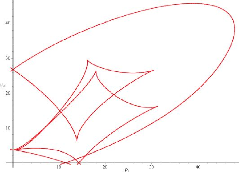
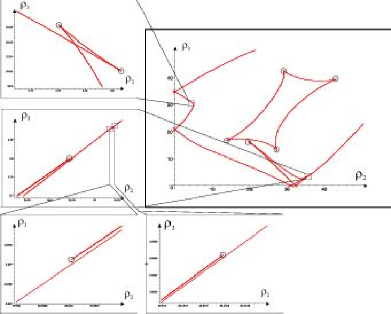
From Table 3 we conclude that, asymptotically, the manipulator has cuspidal configurations, and that this number is stable as soon as is greater than . Moreover, we can observe that the robot may have up to 10 cuspidal configurations when is in the interval . Figure 5 shows the singular curve of the parallel robot for and the corresponding 10 cuspidal configurations.
5 Conclusion
This paper shows that efficient algebraic tools can be applied to analyse in a certified way important kinematic features of parallel manipulators such as the determination of cusp points. These points are known to play an important role in planning non-singular assembly mode changing motions.
A new method was introduced, which is able to characterize all the cusp points for the 3-RPR manipulators. It allowed us to determine the number of cusp points for all the slices of the joint space. For the first time, a section for a given was found with 10 cusp points.
Table 4 summarizes the method used in this article and relates it to the 2 previous main methods to compute cuspidal configurations in the literature.
This results can be computed with a toolbox available now in Maple 12 and later versions [27].
|
|||||||||
|---|---|---|---|---|---|---|---|---|---|
|
|
|
|||||||
\cdashline2-4
|
|||||||||
|
|||||||||
|
|||||||||
|
Discriminant Variety of | ||||||||
Acknowledgement
We would like to thank the reviewers for their useful remarks, which we have all taken into account.
References
- [1] C. M. Gosselin and J.-P. Merlet. The direct kinematics of planar parallel manipulators: Special architectures and number of solutions. Mechanism and Machine Theory, 29(8):1083 – 1097, 1994.
- [2] P. Wenger. Classification of 3R positioning manipulators. Journal of Mechanical Design, 120:327, 1998.
- [3] P. Borrel and A. Liegeois. A study of multiple manipulator inverse kinematic solutions with applications to trajectory planning and workspace determination. In Preceedings of the IEEE International Conference on Robotics and Automation, volume 3, pages 1180–1185, 1986.
- [4] K. H. Hunt and E. J. F. Primrose. Assembly configurations of some in-parallel-actuated manipulators. Mechanism and Machine Theory, 28(1):31–42, 1993.
- [5] C. Innocenti and V. Parenti-Castelli. Singularity-free evolution from one configuration to another in serial and fully-parallel manipulators. Journal of Mechanical Design, 120(1):73–79, 1998.
- [6] P. R. McAree and R. W. Daniel. An explanation of never-special assembly changing motions for 3-3 parallel manipulators. I. J. Robotic Res, 18(6):556–574, 1999.
- [7] X. Kong and C. Gosselin. Type synthesis of 5-DOF parallel manipulators based on screw theory. J. Field Robotics, 22(10):535–547, 2005.
- [8] E. Macho, O. Altuzarra, C. Pinto, and A. Hernandez. Singularity free change of assembly mode in parallel manipulators. Application to the 3-RPR planar platform. 12th IFToMM World Congr., Besancon, France, 2007.
- [9] M. L. Husty. Non-singular assembly mode change in 3-RPR-parallel manipulators. In Computational Kinematics: Proceedings of the 5th International Workshop on Computational Kinematics, page 51. Springer Verlag, 2009.
- [10] H. Bamberger, A. Wolf, and M. Shoham. Assembly mode changing in parallel mechanisms. IEEE Transactions on Robotics, 24(4):765–772, 2008.
- [11] M. Zein, P. Wenger, and D. Chablat. Singular curves in the joint space and cusp points of 3-rpr parallel manipulators. Robotica, 25(6):717–724, 2007.
- [12] CM Gosselin, J. Sefrioui, and MJ Richard. Solutions polynomiales au problème de la cinématique directe des manipulateurs parallèles plans à trois degrés de liberté. Mechanism and machine theory, 27(2):107–119, 1992.
- [13] I. A. Bonev, D. Zlatanov, and C. M. Gosselin. Singularity analysis of 3-DOF planar parallel mechanisms via screw theory. Journal of Mechanical Design, 125:573, 2003.
- [14] J. El Omri and P. Wenger. How to recognize simply a non-singular posture changing 3-dof manipulator. In Proc. 7th Int. Conf. on Advanced Robotics, pages 215–222, 1995.
- [15] S. Corvez and F. Rouillier. Using computer algebra tools to classify serial manipulators. In Automated Deduction in Geometry, pages 31–43, 2002.
- [16] T. Becker and V. Weispfenning. Gröbner bases, volume 141 of Graduate Texts in Mathematics. Springer-Verlag, New York, 1993.
- [17] D. Lazard and F. Rouillier. Solving parametric polynomial systems. J. Symb. Comput., 42(6):636–667, 2007.
- [18] C. Gosselin and J. Angeles. Singularity analysis of closed-loop kinematic chains. IEEE Journal of Robotics and Automation, 6(3):281–290, June 1990.
- [19] M. Elkadi and B. Mourrain. Introduction à la résolution des systèmes d’équations algébriques, volume 59 of Mathématiques et Applications. Springer-Verlag, 2007.
- [20] D. Cox, J. Little, and D. O’Shea. Using algebraic geometry, volume 185 of Graduate Texts in Mathematics. Springer-Verlag, 1998.
- [21] F. Rouillier. Solving zero-dimensional systems through the rational univariate representation. Appl. Algebra Eng. Commun. Comput, 9(5):433–461, 1999.
- [22] D. Eisenbud. Commutative algebra with a view toward algebraic geometry, volume 150 of Graduate Texts in Mathematics. Springer-Verlag, New York-Berlin-Heidelberg-London-Paris-Tokyo-Hong Kong-Barcelona-Budapest, 1994.
- [23] J.-C. Faugere. A new efficient algorithm for computing Gröbner bases (F4). Journal of pure and applied algebra, 139(1-3):61–88, 1999.
- [24] J.-P. Merlet. Parallel Robots, volume 74 of Solid Mechanics and its Applications. Kluwer Academic Publishers, Boston, 2000. INRIA.
- [25] D. Cox, J. Little, and D. O’Shea. Ideals, Varieties, and Algorithms. Undergraduate Texts in Mathematics. Springer Verlag, 1992.
- [26] J.-C. Faugère, G. Moroz, F. Rouillier, and M. Safey El Din. Classification of the perspective-three-point problem, discriminant variety and real solving polynomial systems of inequalities. In Proceedings of the 2008 International Symposium on Symbolic and Algebraic Computation, 2008.
- [27] S. Liang, J. Gerhard, D. J. Jeffrey, and G. Moroz. A Package for Solving Parametric Polynomial Systems. Communication in Computer Algebra, 43(3):61, Septembre 2009.