CMB spectra and bispectra calculations: making the flat-sky approximation rigorous

Abstract

This article constructs flat-sky approximations in a controlled way in the context of the cosmic microwave background observations for the computation of both spectra and bispectra. For angular spectra, it is explicitly shown that there exists a whole family of flat-sky approximations of similar accuracy for which the expression and amplitude of next to leading order terms can be explicitly computed. It is noted that in this context two limiting cases can be encountered for which the expressions can be further simplified. They correspond to cases where either the sources are localized in a narrow region (thin-shell approximation) or are slowly varying over a large distance (which leads to the so-called Limber approximation).

Applying this to the calculation of the spectra it is shown that, as long as the late integrated Sachs-Wolfe contribution is neglected, the flat-sky approximation at leading order is accurate at 1% level for any multipole.

Generalization of this construction scheme to the bispectra led to the introduction of an alternative description of the bispectra for which the flat-sky approximation is well controlled. This is not the case for the usual description of the bispectrum in terms of reduced bispectrum for which a flat-sky approximation is proposed but the next-to-leading order terms of which remain obscure.

I Introduction

Cosmological surveys in general and the cosmic microwave background (CMB) in particular are naturally constructed on our celestial sphere. Because of the statistical isotropy of such observations, cosmological statistical properties, such as the angular power spectra or the bispectra, are better captured in reciprocal space, that is in harmonic space. In general however, most of the physical mechanisms at play take place at small scale and are therefore not expected to affect the whole sky properties. For instance, the physics of the CMB is, to a large extent, determined by sub-Hubble interactions corrsponding to sub-degree scale on our observed sky. Decomposition in spherical harmonics, while introducing a lot of complication of the calculations, does not carry much physical insight into these mechanisms so rather blurs the physics at play.

In this respect, a flat-sky approximation, in which the sky is approximated by a 2-dimensional plane tangential to the celestial sphere, hence allowing the use of simple Cartesian Fourier transforms, drastically simplifies CMB computations. Such an approximation is intuitively expected to be accurate at small scales. So far this approximation is mostly based on an heuristic correspondence between the two sets of harmonic basis (spherical and Euclidean) which can be summarized for a scalar valued observable by Zaldarriaga and Seljak (1997); Hu (2000)

$$\Theta({\bm{n}})=\sum a^{\Theta}_{\ell m}Y_{\ell}^{m}(\hat{\bm{n}})\to\int{\rm d}^{2}{\bf l}\Theta({\bf l})e^{{\rm i}{\bf l}.{\bf\theta}}\,.$$ (1)

In the context of CMB computation, the relations between the flat-sky and the full-sky expansions have been obtained at leading order in Ref. Hu (2000). However, its validity for the angular power spectrum and the bispectrum is not yet understood in the general case and the expression and order of magnitude of the next to leading order terms are still to be computed.

The goal of this article is to provide such a systematic construction. In particular, we will show that there exists a two-parameter family of flat-sky approximations for which well-controlled expansions can be built. That allows us to discuss in details their accuracy by performing the computation up to next-to-leading order. In the new route we propose here, we derive the flat-sky expansion directly on the 2-point angular correlation function, instead of relying on the correspondence (1). One of the technical key step is to expand the eigenfunctions of the spherical Laplacian onto the eigenfunctions of the cylindrical Laplacian in order to relate the (true) spherical coordinates on the sky expansion to the cylindrical coordinates of the flat-sky expansion. This approach proves very powerful since it enables to obtain the full series of corrective terms to the flat-sky expansion.

Once the method has been developed, it can be generalized to the polarisation and also to the computation of the bispectrum. In this latter case, depending on the way one chooses to describe the bispectrum, the exact form of the corrective terms has not been obtained but we can still provide an approximation whose validity can be checked numerically.

Before we enter the details of our investigations, and as the literature can be very confusing regarding the flat-sky approximations, let us present the different levels of approximations we are going to use. The reason there exist at all a flat-sky approximation is that the physical processes at play have a finite angular range. In case of the CMB, most of physical processes take place at sub-horizon scales and within the last scattering surface (LSS) (to the exception of the late integrated Sachs-Wolfe effect) and therefore within 1 degree scale on the sky. Let us denote $\ell_{0}$ the scale, in harmonic space associated with this angular scale. While using the flat sky approximation, the physical processes will be computed in a slightly deformed geometry (changing a conical region into a cylindrical one) introducing a priori an error of the order of $1/\ell_{0}$ (actually in $1/\ell_{0}^{2}$ depending on the type of source terms as it will be discussed in details below). Another part of the approximation is related to the projection effects which determine the link between physical quantities and observables. It introduces another layer of approximation of purely geometrical origin. For that part the errors behave a priori as $1/\ell$ if $\ell$ is the scale of observation in harmonic space.

The resulting integrals do not lead to factorizable properties as it is the case for exact computations, while a factorization property can be recovered taking advantage of two possible limiting situations. First, for most of the small scale physical processes, one can use the fact that the radial extension of the source is much smaller than its distance from the observer. It is then possible to perform a thin-shell approximation effectively assuming that all sources are at the same distance from the observer.

Another limit case corresponds to the situation in which the source terms are slowly varying and spread over a wide range of distances, as e.g. for galaxy distribution or weak-lensing field. In this case the sources support appears very elongated and it is then possible to use the Limber approximation Limber (1953); Peebles (1980); Loverde and Afshordi (2008) which takes advantage of the fact that contributing wave modes in the radial direction should be much smaller that the modes in the transverse direction (but as such the Limber approximation can be used in conjunction of the flat-sky approximation or not).

These different layers of approximations proved to be useful to compute efficiently the effects of secondaries such as lensing, but also of great help for computing the effects of non-linearities at the LSS contributing to the bispectrum, either analytically Boubekeur et al. (2009); Pitrou et al. (2008) or numerically Pitrou et al. (2010) (see Ref. Nitta et al. (2009) to compare to the full-sky expressions) as well as for the angular power spectrum; see e.g. Ref. Lewis and Challinor (2006) for a review and for the relation between the flat-sky and the full-sky expansions in both real and harmonic space. We shall thus detail the expressions and corrective terms of the flat-sky approximation in these two approximations. In particular, we recover the result by Ref. Loverde and Afshordi (2008) with a different method in the case of the Limber approximation. This is a consistency check of our new method.

First, we consider the computation of the angular power spectrum in Section II starting with an example of such a construction in order to show explicitly how to construct next to leading order terms whose correction is found to be of the order of $1/\ell^{2}$. We then show that this construction is not unique and present the construction of a whole family of approximations whose relationship can be explicitly uncovered. In Section III we present further computation approximations, e.g. the Limber (§ III.1) and thin-shell (§ III.2) approximations. While in Sections II and  III we have assumed, for clarity but also because it changes the result only at next-to-leading order, that the transfer function was scalar, in Section IV we provide the general case of the flat-sky approximation up to next-to-leading order corrections in $1/\ell$ including all physical effects. Eventually Section V considers the case of higher spin quantities to describe the CMB polarization.

We explore the case of the bispectrum construction in Section VI. One issue we encountered here is that different equivalent parameterizations can be used to describe bispectra (amplitudes of bispectra depend on both the scale and shape of the triangle formed by three $\ell$ modes that can be described in different manners). We thus present an alternative description of the bispectrum for which the flat-sky approximation can be done in a controlled way. Although we did not do the calculation explicitly, next-to-leading order terms can be then obtained. This is not the case for the reduced bispectrum for which we could nonetheless propose a general flat-sky approximation. Similarly to the case of spectra practical computations can then be done in the thin-shell approximation or the Limber approximation.

II Power spectrum in the flat-sky limit

II.1 General definitions

In the line of sight approach, the temperature $\Theta({\bm{\hat{}}{n}})$ observed in a direction ${\bm{\hat{}}{n}}$ is expressed as the sum of all emitting sources along the line of sight in direction ${\bm{\hat{}}{n}}$,

$$\Theta({\bm{\hat{}}{n}})=\int{\rm d}r\int\frac{{\rm d}^{3}{\bm{k}}}{(2\pi)^{3/2}}\,w({\bm{k}},{\bm{\hat{}}{n}},r)\Phi({\bm{k}})\exp({\rm i}{\bm{k}}.{\bm{x}})\,,$$ (2)

where ${\bm{x}}$ is the position at distance $r$ and angular position $(\theta,\varphi)$ and $\Phi$ is the primordial gravitational potential from which all initial conditions can be constructed Ma and Bertschinger (1995). $w({\bm{k}},{\bm{\hat{}}{n}},r)$ is a transfer function that depends on both the wave-number ${\bm{k}}$ and the direction of observation ${\bm{\hat{}}{n}}$. In particular, it incorporates altogether the visibility function, $\tau^{\prime}e^{-\tau}$, where $\tau$ is the optical depth, and the time and momentum dependencies of the sources. It can always be expanded as

$$w({\bm{k}},\hat{\bm{n}},r)=\sum_{j,m}w_{jm}(k,r)({\rm i})^{j}\sqrt{\frac{4\pi}{2j+1}}Y_{{\bm{k}}}^{jm}(\hat{\bm{n}})$$ (3)

where the $Y_{{\bm{k}}}^{jm}$ are the spherical harmonics with azimutal direction aligned with ${\bm{k}}$. The source multipoles are defined using the same conventions as in Refs. Hu and White (1997); Pitrou (2009) except that the multipoles are defined here using the direction of observation whereas in these references it is defined with the direction of propagation . As long as we consider only scalar type perturbations in the perturbation theory, the source term will only contain $w_{jm}$ terms with $m=0$. For instance, the Doppler term of the scalar perturbation introduces a term $w_{10}$ etc.

In order to focus our attention to the geometrical properties of the flat-sky expansion, we first assume for simplicity that the temperature fluctuations do not depend on ${\bm{\hat{}}{n}}$ and are thus only scalar valued functions. The statistical isotropy of the primordial fluctuations then implies that the ${\bm{k}}$-dependency reduces to a $k$-dependency, so that the transfer function is of the form $w(k,r)=w_{00}$. The general case is postponed to Section IV.

The two-point angular correlation function of the temperature anisotropies, defined by

$$\xi(\theta)=\langle\Theta({\bm{\hat{}}{n}})\Theta({\bm{\hat{}}{n}}^{\prime})\rangle_{{\bm{\hat{}}{n}}.{\bm{\hat{}}{n}}^{\prime}=\cos\theta}\,,$$ (4)

is related to the angular power spectrum $C_{\ell}$ by

$$C_{\ell}=2\pi\int\sin\theta{\rm d}\theta\,P_{\ell}(\cos\theta)\,\xi(\theta),$$ (5)

where $P_{\ell}$ are the Legendre polynomials of order $\ell$. The 3-dimensional power spectrum of the primordial potential being defined by

$$\langle\Phi({\bm{k}})\Phi({\bm{k}}^{\prime})\rangle=\delta({\bm{k}}+{\bm{k}}^{\prime})P(k)\,,$$ (6)

we can easily invert this relation to get a one-parameter family of correlation functions $\xi_{v}(\theta)$ as

$$\qquad\xi_{v}(\theta) = \int\frac{{\rm d}k_{r}}{(2\pi)^{2}}\ k_{\perp}{\rm d}k_{\perp}w(k,r)w^{\star}(k,r^{\prime}){\rm d}r{\rm d}r^{\prime}$$ (7)

$$\times P(k)J_{0}\left[k_{\perp}\left(r^{\prime}\sin v\theta+r\sin(1-v)\theta\right)\right]$$

$$\times \exp\left[{\rm i}k_{r}\left(r\cos(1-v)\theta-r^{\prime}\cos v\theta\right)\right]\,$$

where $J_{0}$ is the Bessel function of the first kind of order $0$ and where the star denotes the complex conjugation. The index $v$ refers to the parametrization according to the two line-of-sight

$${\bm{x}} = r[\sin((1-v)\theta){\bm{n}}_{\perp},\cos((1-v)\theta)]$$ (8)

$${\bm{x}}^{\prime} = r^{\prime}[\sin(v\theta){\bm{n}}^{\prime}_{\perp},\cos(v\theta)]\,,$$

where we have defined the two-dimensional vectors ${\bm{n}}_{\perp}\equiv(\cos\varphi,\sin\varphi)$ and ${\bm{n}}^{\prime}_{\perp}\equiv(\cos(\varphi+\psi),\sin(\varphi+\psi))$ with $\psi=\pi$ so that ${\bm{n}}^{\prime}_{\perp}=-{\bm{n}}_{\perp}$. Note that the relation (7) has been obtained for a fixed value of $\psi$, the relative angle between ${\bm{n}}^{\prime}_{\perp}$ and ${\bm{n}}_{\perp}$, although it could have been left as a free parameter. As we will see in the following, flat-sky approximations can indeed be obtained for any fixed value of $v$ and $\psi$ provided ${\bm{\hat{}}{n}}$ and ${\bm{\hat{}}{n}}^{\prime}$ are close enough to the azimuthal direction. In the last part of II.3 we will briefly comment on the effect of considering $\psi$.

Any Fourier mode ${\bm{k}}$ can then be decomposed into a component $k_{r}$ orthogonal to ${\bm{n}}_{\perp}$ and a component ${\bm{k}}_{\perp}$ parallel to ${\bm{n}}_{\perp}$. Its modulus $k$ is thus to be considered as a function of $k_{r}$ and $k_{\perp}$ since

$$k=\sqrt{k_{r}^{2}+k_{\perp}^{2}}\,.$$ (9)

To finish, we parameterize ${\bm{k}}_{\perp}$ as

$${\bm{k}}=(k_{\perp}\cos\beta,k_{\perp}\sin\beta,k_{r})\,.$$ (10)

Note that the Bessel function in the expression (7) arises from the integration over the angle between ${\bm{k}}_{\perp}$ and ${\bm{n}}_{\perp}$, i.e. $\beta-\varphi$. This requires to assume that the transfer function depends neither on $\hat{\bm{k}}={\bm{k}}/k$ nor on ${\bm{\hat{}}{n}}$ and is thus independent of the angle between ${\bm{k}}_{\perp}$ and ${\bm{n}}_{\perp}$. Note that for simplicity we could have chosen to set $\varphi=0$ since only the relative angle between ${\bm{k}}_{\perp}$ and ${\bm{n}}_{\perp}$ matters in the derivation of the result.

II.2 A construction case: the $v=0$ case

Before investigating the full family $\xi_{v}$ in the flat-sky limit, let us concentrate on the particular case $v=0$. The flat-sky approximation is obtained as a small angle limit, i.e. $\theta\ll 1$ while letting ${\alpha_{\ell}}=\ell\theta$ fixed. In order to expand the Legendre polynomials $P_{\ell}(\cos\theta)$ in that limit, we start from their integral representation as

$$P_{\ell}(\cos\theta)=\frac{1}{\pi}\int_{0}^{\pi}\exp\left[\ell\log\left(\cos\theta+{\rm i}\sin\theta\cos\varphi\right)\right]{\rm d}\varphi.$$ (11)

In the above mentioned limit, it gives the integral representation of $J_{0}(\ell\theta)$,

$$J_{0}(\ell\theta)=\frac{1}{\pi}\int_{0}^{\pi}\exp\left[{\rm i}\ell\theta\cos\varphi\right]{\rm d}\varphi\,.$$ (12)

Furthermore, it allows to obtain the subsequent terms of the expansion as

$$P_{\ell}(\cos\theta) = J_{0}({{\alpha_{\ell}}})$$

$$- \frac{\theta}{2}J_{1}({{\alpha_{\ell}}})-\frac{\theta^{2}}{24}J_{0}({{\alpha_{\ell}}})+\frac{\theta^{2}}{12\,{{\alpha_{\ell}}}}J_{1}({{\alpha_{\ell}}})+\dots,$$

again for a fixed ${{\alpha_{\ell}}}\equiv\ell\theta$. The existence of such an expansion, and its simplicity, is central in the construction we present here. It shows that the eigenfunctions of the Laplacian on the 2-sphere converge toward eigenfunctions of the Laplacian on the Euclidean plane.

This expansion is however not optimal. It was already pointed out in Refs. Bond (1996); Seljak (1997); Loverde and Afshordi (2008) that it can be improved by choosing the argument of the Bessel functions to be ${{\alpha_{L}}}=L\theta$ with

$$L\equiv\ell+\frac{1}{2}\,,$$ (14)

instead of $\ell\theta$. The novel expansion can easily be obtained by shifting the argument of the Bessel function in the right hand side of the relation (II.2). It then reads to second order,

$$P_{\ell}(\cos\theta) = J_{0}({{\alpha_{L}}})$$ (15)

$$+ \left(\frac{\theta}{2}\right)^{2}\left[\frac{J_{0}({{\alpha_{L}}})}{3}-\frac{J_{1}({{\alpha_{L}}})}{6{{\alpha_{L}}}}\right]+\dots$$

The correction term in $\sim\theta$ of the expansion (II.2) has indeed disappeared and, as a consequence, the first correction to the lowest order of the flat-sky expansion is expected to scale as $\ell^{-2}$, (in the sense discussed below). The accuracy of this mapping is numerically illustrated in Fig. 1 for $\ell=4$ and $\ell=20$, and shown to be better than the percent level. As can be appreciated from this expression, from this figure and Fig. 3 later on, this change of expansion point is a very important step that eventually justifies the use of the flat-sky approximation in the context of precision calculations.

Figure 1: Accuracy of the expansions (II.2) in thin lines and (15) in thick lines. We plot the difference between $P_{l}(\cos\theta)$ and its approximate forms, at leading order in $\theta$ (i.e. $J_{0}(l\theta)$, solid lines), first order (long dashed lines), second order (short dashed lines) for $\ell=4$ and as a function of $\theta$ (left) and $\ell=20$ (right).

Finally it is to be noticed that in order to use correctly the orthogonality relations of the Bessel functions, it is necessary to use the variable

$$Z \equiv 2\tan\left(\theta/2\right)$$ (16)

instead of $\theta$ since $Z$ runs to infinity when $\theta\to\pi$. The expansion of $P_{\ell}(\cos\theta)$ in function of ${\hat{\alpha}_{L}}=LZ$ reads

$$P_{\ell}(\cos\theta)=J_{0}({\hat{\alpha}_{L}})$$ (17)

$$+\left(\frac{{\hat{\alpha}_{L}}}{2L}\right)^{2}\left[\frac{J_{0}({\hat{\alpha}_{L}})}{3}-\frac{J_{1}({\hat{\alpha}_{L}})}{6{\hat{\alpha}_{L}}}+\frac{{\hat{\alpha}_{L}}J_{1}({\hat{\alpha}_{L}})}{3}\right]+\dots$$

We are then in position to derive the expression of the angular power spectrum in the flat-sky limit. The starting point is the expression (7) of the correlation function where the $\theta$-dependent part of the integrand is expanded as $\exp\left[{\rm i}k_{r}(r-r^{\prime})\right]J_{0}(k_{\perp}r\theta)+{\cal O}(\theta^{2})$. This can then be plugged into Eq. (5), using the expansion (15) of the Legendre polynomials and integrated over ${\hat{\alpha}_{L}}$, using Eqs.  (136-137) to give, up to terms in $\ell^{-2}$,

$$C^{(v=0)}_{\ell}=\frac{1}{2\pi}\int{\rm d}r{\rm d}r^{\prime}{\rm d}k_{r}k_{\perp}{\rm d}k_{\perp}\frac{\exp[{\rm i}k_{r}(r-r^{\prime})]}{r^{2}}P(k)w(k,r)w^{\star}(k,r^{\prime})\times$$ (18)

$$\left[I_{0,0}(L/r,k_{\perp})-\frac{5}{12r^{2}}I_{0,1}(L/r,k_{\perp})-\frac{1}{6Lr}I_{1,0}(L/r,k_{\perp})+\frac{L}{12r^{3}}I_{1,1}(L/r,k_{\perp})+\frac{k_{\perp}}{4r^{2}}I_{1,1}(k_{\perp},L/r)-\frac{{\rm i}k_{r}}{2r}I_{0,1}(k_{\perp},L/r)\right],$$

where the functions $I_{n,p}$ are defined in the appendix A. Integrating on $k_{\perp}$, we finally get after integrations by parts

$$C^{(v=0)}_{\ell} = \frac{1}{2\pi}\int{\rm d}r{\rm d}r^{\prime}{\rm d}k_{r}\frac{\exp[{\rm i}k_{r}(r-r^{\prime})]}{r^{2}}\left[1+\frac{1}{24L^{2}}\left(D_{\perp}-6D_{\perp}^{2}-4D_{\perp}^{3}\right)+\frac{{\rm i}k_{r}r}{2L^{2}}D_{\perp}^{2}\right]P(k)w(k,r)w^{\star}(k,r^{\prime})\,,$$ (19)

where $D_{\perp}\equiv\partial/\partial\ln k_{\perp}$ acts on all the terms on its right, and where $k^{2}=k_{r}^{2}+L^{2}/r^{2}$. This means that we must impose the constraint

$$k_{\perp}r=L\,.$$ (20)

Higher order corrections will introduce higher order derivatives of $P(k)w(k,r)w(k,r^{\prime})$ with respect to $k_{\perp}$. Since the function on which the derivative acts is only a function of $k$, it is understood in the above expression, and in the rest of this paper, that $\partial_{k_{\perp}}=(k_{\perp}/k)\,\partial_{k}$. The evolution of the sources is mainly due to the baryon acoustic oscillations and thus $\partial\ln w(k,r)/\partial k\sim\eta_{{\textrm{LSS}}}$ where $\eta_{\textrm{LSS}}$ is the mean time of the last scattering surface. If the initial power spectrum is a power law, $\partial\ln P(k)/\partial k\propto 1/k$. For super-Hubble scales at the time of recombination, the corrective terms are dominated by the variations of $P(k)$ whereas on sub-Hubble scales, they are dominated by the variation of the transfer function. We thus have

$$\partial_{k}\ln\left[P(k)w(k,r)w^{\star}(k,r^{\prime})\right]\propto\left\{\begin{array}[]{ll}1/k&{\rm if}\,\,\,k\eta_{{\textrm{LSS}}}\ll 1\\ \eta_{{\textrm{LSS}}}&{\rm if}\,\,\,k\eta_{{\textrm{LSS}}}\gg 1.\end{array}\right.$$ (23)

The scaling of the corrective term can then be inferred easily. If $\Delta r_{\textrm{LSS}}$ is the typical width of the last scattering surface, the exponential term in the integral on $k_{r}$ imposes the constraint $k_{r}\Delta r_{\textrm{LSS}}\lesssim 1$. Now, since the power spectrum should be decreasing faster than $k^{-2}$ for large $k$, the dominant contribution to the integral arises from $k_{r}\lesssim k_{\perp}$. We thus conclude that $k_{r}\lesssim{\rm min}(k_{\perp},\Delta r_{\textrm{LSS}})$ and that we always have $k\approx k_{\perp}$. In the small scale regime, that is for $\ell\gg r_{{\textrm{LSS}}}/\eta_{\textrm{LSS}}\approx 50$ ($r_{\textrm{LSS}}\equiv\eta_{0}-\eta_{\textrm{LSS}}$ being the average comoving distance to the last scattering surface) then $k\eta_{{\textrm{LSS}}}\ll 1$. According to Eq. (23), this means that the first corrective term is, in this regime, of order $(\eta_{{\textrm{LSS}}}/r_{{\textrm{LSS}}})^{2}\sim{\cal O}(10^{-4})$. In the large scale regime, $\ell\ll r_{{\textrm{LSS}}}/\Delta r_{\textrm{LSS}}$, and thus $k\approx k_{r}\approx k_{\perp}$. Since for these modes $\ell\ll r_{\textrm{LSS}}/\eta_{\textrm{LSS}}$, then $k\eta_{\textrm{LSS}}\ll 1$, and this implies that the first corrective term scales approximately as $1/\ell^{2}$.

Concerning the higher order expansion of Eq. (19), we see that a corrective term of order $1/L^{n}$ will involve the operator $D_{\perp}^{p}/L^{n}$ where $p$ can be any integer, which gives formally a systematic way of organizing the expansion to any order.

To summarize, the precision of the lowest order flat-sky approximation in the context of CMB calculations is of order $1/\ell^{2}$ for $\ell\lesssim 50$ and limited to $10^{-4}$ level for $\ell\gtrsim 50$, i.e. they are of order ${\rm max}(\ell^{-2},\ell_{0}^{-2})$ with $\ell_{0}=50$. We refer to this first correction as being the correction of order $1/\ell^{2}$, even if it is limited for small scales because of the sub-horizon physics .

We finally note that in some cases the results can actually be further improved by choosing the argument of the Bessel functions to be ${\alpha_{\tilde{L}}}\equiv\tilde{L}\theta\equiv\sqrt{l(l+1)}\theta$, since then

$$\quad P_{\ell}(\cos\theta) = J_{0}({\alpha_{\tilde{L}}})$$

$$+\left(\frac{{\alpha_{\tilde{L}}}}{2\tilde{L}}\right)^{2}\left[\frac{J_{0}({\alpha_{\tilde{L}}})}{3}-\frac{2J_{1}({\alpha_{\tilde{L}}})}{3{\alpha_{\tilde{L}}}}\right]+\dots\,.$$

Indeed, this expansion also removes the corrections scaling as $\ell^{-1}$ in Eq. (19) since it also does not contain terms linear in $\theta$. Now, the flat-sky constraint reads

$$k_{\perp}r=\tilde{L}=\sqrt{\ell(\ell+1)}\,.$$ (25)

With this choice, it appears that for any transfer function $w(k,r)$ that is constant and sharply peaked, i.e. that is such as $w(k,r)=\delta(r-r_{\textrm{LSS}})$, and for a scale invariant power spectrum, i.e. $P(k)=2\pi^{2}A_{s}^{2}k^{-3}$, the lowest order in the flat-sky expansion takes the form

$$C_{\ell}=\int\frac{{\rm d}k_{r}}{2\pi}\frac{1}{r_{\textrm{LSS}}^{2}}P(k)=\frac{2\pi A_{s}^{2}}{\ell(\ell+1)}\,.$$ (26)

This is precisely the result that one would have obtained with the exact (or full spherical sky) calculation since

$$\qquad C_{\ell}=\frac{2}{\pi}\int{\rm d}kk^{2}P(k)\left[j_{\ell}(kr_{\textrm{LSS}})\right]^{2}=\frac{2\pi A_{s}^{2}}{\ell(\ell+1)}\,.$$

In other words, with this choice, the leading term of the flat-sky expansion is exact. For CMB on large scales, this is precisely the case since super-Hubble perturbations are frozen, leading to the Sachs-Wolfe plateau. Given that the initial power spectrum is expected to be almost scale-invariant, we conclude that this expansion of $P_{\ell}(\cos\theta)$ is the best one in the context of CMB computations and we usually adopt it. We can argue that the choice $kr=L$ is more compact while the choice $kr=\tilde{L}$ gives a better formula only in the thin-shell approximation. In appendix B we explain how to change the constraint inside the expressions obtained. In general however, one cannot state which is the best choice and in the following, unless stated otherwise, we will use only $L$.

II.3 Generalized flat-sky expansions

The derivation of the previous section was limited to the case $v=0$ but, as it appears clearly from the parameterizations (8), it is actually possible to build a two-parameter family of flat-sky approximations, the relation between which should be examined.

II.3.1 A one-parameter family of flat-sky approximations

The aim of this subsection is to explore the consequence of the use of a more general parameterization (8) introducing $v$ as a free parameter. Note that we still keep $\psi=\pi$ although it could be reintroduced at this stage too. Calculations for arbitrary values of $\psi$ are however significantly more complicated and do not lead to any improved scheme. Then, again, the particular cases $v=0$ or $v=1$ correspond to $\hat{\bm{n}}_{z}\equiv(0,0,1)$ aligned either with $\hat{\bm{n}}$ or $\hat{\bm{n}}^{\prime}$ and the case $v=1/2$ to $\hat{\bm{n}}_{z}$ aligned with $(\hat{\bm{n}}+\hat{\bm{n}}^{\prime})/\sqrt{2}$.

We can now follow the same approach as in section II.2. The expansion in powers of $Z$ (instead of $\theta$) can be performed with the variables $\Delta\equiv r-r^{\prime}$ and

$$R\equiv r^{\prime}v+(1-v)r.$$ (27)

Plugging the expansion (17) into Eq. (5) with the definition (7) of the correlation function, one can perform an expansion in $Z$ and $\Delta$, and then, using the orthonormality relations of appendix A we can compute the integral on $\tilde{{\alpha_{L}}}$ in function of the $I_{n,p}(k_{\perp},L/R)$. Eventually the result reads

$$C^{(v)}_{\ell}=\int\frac{{\rm d}r{\rm d}r^{\prime}{\rm d}k_{r}}{2\pi}\frac{\exp({\rm i}k_{r}\Delta)}{R^{2}}{\cal O}^{(v)}_{k_{\perp}}P(k)w(k,r)w^{\star}(k,r^{\prime})\,,$$ (28)

where ${\cal O}^{(v)}_{k_{\perp}}$ is an operator that applies on the right part of the previous expression with

$${\cal O}^{(v)}_{k_{\perp}}=1+\frac{D_{\perp}}{24L^{2}}-[(4-3f_{1/2})R+f_{1/2}f_{0}\Delta]\frac{D_{\perp}^{3}}{24RL^{2}}$$

$$-[f_{1/2}f_{0}\Delta+3Rf_{0}^{2}]\frac{D_{\perp}^{2}}{12RL^{2}}+{\rm i}k_{r}(4f_{0}R+f_{1/2}\Delta)\frac{D_{\perp}^{2}}{8L^{2}}$$ (29)

where $f_{1/2}\equiv 4v(1-v)$, $f_{0}=1-2v$ and

$$D_{\perp}\equiv k_{\perp}\frac{\partial}{\partial k_{\perp}}=\frac{k_{\perp}^{2}}{k}\frac{\partial}{\partial k}=\frac{L^{2}}{kR^{2}}\frac{\partial}{\partial k}\,.$$ (30)

Besides the $v=0$ case for which this expression simplifies, this is also the case for the symmetric choice, $v=1/2$, for which it leads to,

$$C^{(v=1/2)}_{\ell}=\int\frac{{\rm d}r{\rm d}r^{\prime}{\rm d}k_{r}}{2\pi}\frac{\exp({\rm i}k_{r}\Delta)}{R^{2}}\left[1+\frac{1}{24L^{2}}\left(D_{\perp}-D_{\perp}^{3}\right)+\frac{{\rm i}k_{r}\Delta}{8L^{2}}D_{\perp}^{2}\right]P(k)w(k,r)w^{\star}(k,r^{\prime})\,.$$ (31)

The lowest order of this expression matches the one derived in Ref. Bond (1996). We remind that the constraint $k_{\perp}R=L$ must be satisfied and that this expression is valid only up to order $L^{-2}$. In the general case for which $v\not=1/2$, at lowest order in the flat-sky expansion, the expression would remain formally the same, considering that $R$ would then be given by $R=r^{\prime}v+(1-v)r$. We will compare these different parameterizations in the following paragraph. However, if we also take into account the corrections, the choice of $v$ would change the expression of the flat-sky expansion. In appendix B we detail how the different corrections obtained are consistent with one another.

II.3.2 Breaking of statistical isotropy and off diagonal contributions

The existence of mathematically equivalent flat-sky approximations may appear surprising at first view (at least it surprised the authors) but it can be fully understood when one addresses the construction of the correlators in harmonic space not assuming the statistical isotropy of the sky.

Indeed an important consequence of the flat-sky approximation is, because a particular direction has been singled out, to break the statistical isotropy of the sky. There is therefore no reason to have, $C_{\ell_{1}m_{1}\ell_{2}m_{2}}=C_{\ell_{1}}\delta_{\ell_{1}\ell_{2}}\delta_{m_{1}m_{2}}$ at any order in flat-sky approximation where $C_{\ell_{1}m_{1}\ell_{2}m_{2}}$ is the ensemble average of the product of two spherical harmonics coefficients.

In terms of the two-point angular correlation functions we have in general,

$$C_{\ell_{1}m_{1}\ell_{2}m_{2}}\equiv\int{\rm d}\hat{\bm{n}}_{1}{\rm d}\hat{\bm{n}}_{2}\xi(\hat{\bm{n}}_{1},\hat{\bm{n}}_{2})Y_{\ell_{1}}^{m_{1}}(\hat{\bm{n}}_{1})Y_{\ell_{2}}^{\star m_{2}}(\hat{\bm{n}}_{2})\,,$$ (32)

where $\xi(\hat{\bm{n}}_{1},\hat{\bm{n}}_{2})$ is the correlation function of two given directions. The difference with Eq. (4) is that we have not assumed isotropy. If we choose these two directions to be close to a common direction $\hat{\bm{n}}$, then we can expand the spherical harmonics of Eq. (32) around that direction which is chosen to be aligned with the azimuthal direction and this step breaks explicitly the isotropy of the problem. At lowest order, this gives (see appendix C)

$$Y_{\ell}^{m}(\hat{\bm{n}})\simeq\sqrt{\frac{2\ell+1}{4\pi}}(-1)^{m}J_{m}(\ell\theta)e^{{\rm i}m\varphi}.$$

It implies that

$$C_{\ell_{1}m_{1}\ell_{2}m_{2}}\simeq\delta_{m_{1}m_{2}}C_{\ell_{1}\ell_{2}},$$ (33)

as a consequence of the preservation of the statistical rotational invariance around the particular direction ${\bm{\hat{}}{n}}$. The term $C_{\ell_{1}\ell_{2}}$ is explicitely given by

$$C_{\ell_{1}\ell_{2}}\equiv\frac{1}{2\pi}\int{\rm d}r_{1}{\rm d}r_{2}{\rm d}k_{\perp}k_{\perp}{\rm d}k_{r}P(k)w(k,r_{1})w^{\star}(k_{,}r_{2})$$

$$\quad\times\exp[{\rm i}k_{r}(r_{1}-r_{2})]\frac{\delta(k_{\perp}r_{1}-L_{1})\delta(k_{\perp}r_{2}-L_{2})}{\sqrt{L_{1}L_{2}}}$$ (34)

where we remind that $L\equiv\ell+1/2$ (or $=\sqrt{\ell(\ell+1)}$). Performing the integrals on $r_{1}$ and $r_{2}$ leads to

$$C_{\ell_{1}\ell_{2}} \equiv \frac{1}{2\pi}\int\frac{{\rm d}k_{\perp}}{k_{\perp}}{\rm d}k_{r}P(k)\exp\left[{\rm i}(L_{1}-L_{2})\frac{k_{r}}{k_{\perp}}\right]$$ (35)

$$\qquad\times\frac{w\left(k,\frac{L_{1}}{k_{\perp}}\right)w^{\star}\left(k,\frac{L_{2}}{k_{\perp}}\right)}{\sqrt{L_{1}L_{2}}}\,.$$

In Fig 2 we present $C_{\ell_{1}\ell_{2}}$ in the space of $(\ell_{1}+\ell_{2})/2$ and $(\ell_{1}-\ell_{2})/2$. The main power is carried by multipoles such that $\ell_{1}\approx\ell_{2}$. The difference between the different possible flat-sky approximations lies precisely in the existence of (small) off-diagonal terms.

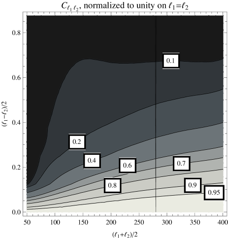
Figure 2: $C_{\ell_{1}\ell_{2}}/C_{\ell_{+}\ell_{+}}$ with $\ell_{+}=(L_{1}+L_{2})/2-1$. Most of the signal is localized on the diagonal $L_{1}=L_{2}$. The choice of the path of integration in this space leads to different flat-sky expansions, that is to different choices of the flat-sky direction ${\bm{\hat{}}{n}}$ or equivalently of the parameter $v$. For $v=0$ or $v=1$, the lowest order of Eq. (19) can be recovered by integrating on an horizontal or a vertical line in the $(L_{1},L_{2})$ plane. As for $v=1/2$, the lowest order of the expression (31) is recovered by integrating on the line $L_{1}+L_{2}=$const. The vertical black line(s) is the superposition of those various integration paths for $L=280$. On the plot they are hardly distinguishable.

II.3.3 Recovering the different flat-sky approximations

Interestingly, each $C_{\ell}^{(v)}$ can be recovered by a proper integration of $C_{\ell_{1}\ell_{2}}$, given by Eq. (II.3.2), in the $(\ell_{1},\ell_{2})$-plane. Each path of integration corresponds to a way to relate the correlation function $\xi(\hat{\bm{n}}_{1},\hat{\bm{n}}_{2})$ to $\xi(\theta)$ defined in Eq. (4).

For instance, when $v=0$, the expression (19), which is then the lowest order part of the expression (31), can be recovered by integrating along the path $L_{1}$=const., i.e. as

$$L_{1}C_{\ell_{1}}=\int{\rm d}L_{2}\sqrt{L_{1}L_{2}}C_{\ell_{1}\ell_{2}}.$$ (36)

The integration along $L_{2}$=const. corresponds to the case $v=1$ and gives by symmetry the same result, which was expected since it corresponds to exchanging ${\bm{\hat{}}{n}}_{1}$ and ${\bm{\hat{}}{n}}_{2}$.

The symmetric case $v=1/2$ can be recovered by integrating on the path $L_{1}+L_{2}$=const. Making the change of variables

$$L_{+}=\frac{L_{1}+L_{2}}{2}\,,\qquad L_{-}=\frac{L_{1}-L_{2}}{2}\,,$$ (37)

we thus obtain

$$C_{\ell_{1}} = \int\frac{{\rm d}L_{-}}{2}\frac{\sqrt{L_{1}L_{2}}}{L_{+}}C_{\ell_{1}\ell_{2}}$$ (38)

$$= \int\frac{{\rm d}L_{-}}{2}\sqrt{\left(1-\frac{L_{-}^{2}}{L_{+}^{2}}\right)}C_{\ell_{1}\ell_{2}}\,.$$

Actually, for a general $v$, the lowest order of the expression (31) is recovered by integrating on the path of equation

$$L_{2}/L_{1}=(v-1)/v$$ (39)

in this plane. The case of $\psi\neq\pi$ in Eq. (8) leads to similar constructions but with slightly more complicated integration paths. To show it let us reintroduce $\psi$ in Eq. (8). Then the angular separation $\tilde{\theta}$ of the directions ${\bm{\hat{}}{n}}$ and ${\bm{\hat{}}{n}}^{\prime}$ reads

$$\tilde{\theta}^{2}=(v^{2}+(1-v)^{2}-2v(1-v)\cos\psi)\theta^{2}$$ (40)

and the effective radius $R$ (as it appears in the argument of $J_{0}$) is

$$R^{2}=(r^{2}v^{2}+r^{\prime 2}(1-v)^{2}-2rr^{\prime}v(1-v)\cos\psi)\theta^{2}$$ (41)

with the relation

$$L\tilde{\theta}=k_{\perp}R.$$ (42)

The relation between $L$, $L_{1}$ and $L_{2}$ then follows from the relations $L_{1}=rk_{\perp}$ and $L_{2}=r^{\prime}k_{\perp}$. It reads,

$$L^{2}=\frac{v^{2}L_{1}^{2}+(1-v)^{2}L_{2}^{2}-2v(1-v)\cos\psi L_{1}L_{2}}{v^{2}+(1-v)^{2}-2v(1-v)\cos\psi}$$ (43)

which describes the arc of an ellipse in the $(L_{1},L_{2})$ plane. All these approximations are a priori of similar precision. Note however that when $\psi$ is small, $\theta$ should be large in order to keep $\tilde{\theta}$ fixed making the various expansions less precise. It then corresponds to a very squeezed ellipse in the $(L_{1},L_{2})$ plane.

III Two limit cases

It is worth remarking that in either Eq. (19) or more generally in Eq. (31), the computation of power spectra at leading order involves a genuine 3D numerical integration. It is therefore numerically less favorable than exact calculations (which involves only two integrals Seljak and Zaldarriaga (1996); Hu and White (1997)  .) It is just more transparent since it does not require the computation of spherical Bessel functions, and geometrically more transparent since the results are presented in a Cartesian form.

Depending on the physical situation, it is however possible to introduce simplifications that will make the computations faster.

III.1 The Limber approximation

Let us first consider the situation in which the sources stretch in a wide range of distances $\Delta r$ and vary smoothly. As long as $\ell/r\times\Delta r\gg 1$, it implies that $k_{\perp}\Delta r\gg 1$. As a consequence, the contributions in the integral on $k_{r}$ are approximately ranging from $-1/\Delta r$ to $1/\Delta r$, that is in a range of values where $k=\sqrt{k_{\perp}^{2}+k_{r}^{2}}\simeq k_{\perp}$ and all functions except the exponential in the integrand can be considered constant.

The Limber approximation then consists in replacing

$$\int{\rm d}k_{r}\exp[{\rm i}k_{r}(r-r^{\prime})]$$

by $2\pi\delta{(r-r^{\prime})}$ so that the integral on $r^{\prime}$ can then be performed trivially. We finally obtain, at lowest order in powers of $\ell^{-1}$

$$C_{\ell}=\int{\rm d}r\left|\frac{w(k,r)}{r}\right|^{2}P(k)\,,$$ (44)

with the Limber constraint $kr=L$. The first corrections scale as $L^{-2}$ and have been computed in Ref. Loverde and Afshordi (2008). We can recover this result from Eq. (31), by expanding all functions of $k$ around $k_{\perp}$ as

$$f(k)=f(k_{\perp})+\frac{k_{r}^{2}}{2k_{\perp}}\left.\frac{\partial f(k)}{\partial k}\right|_{k=k_{\perp}}+\dots$$

This will result in a term proportional to $k_{r}^{2}$ which can be handled using

$$\int{\rm d}k_{r}(ik_{r})^{n}\exp[{\rm i}k_{r}\Delta]=2\pi\delta^{\{n\}}(\Delta)\,,$$ (45)

where $\delta^{\{n\}}$ is the $n$-th derivative of the Dirac distribution. The term proportional to $k_{r}$ in Eq. (31) can be handled in the same way and gives $\delta^{\prime}(\Delta)$. Integrating by parts in $\Delta$ removes the derivatives of the Dirac distributions, using that $\partial R/\partial r=1-v$ and $\partial R/\partial r^{\prime}=v$. Then, the integral on $r^{\prime}$ is trivial, because of the Dirac distributions, and one can then perform an integration by parts in $r$ in order to reshape the result. We finally obtain

$$C^{(v=1/2)}_{\ell}=\int\frac{{\rm d}r}{r^{2}}\left\{P(k)\left|w(k,r)\right|^{2}+\frac{D}{2L^{2}}\left[r\left|\frac{\partial\left[w(k,r)/\sqrt{r}\right]}{\partial\ln r}\right|^{2}P(k)\right]-\frac{D^{2}}{2L^{2}}[w(k,r)^{2}P(k)]-\frac{D^{3}}{6L^{2}}[w(k,r)^{2}P(k)]\right\}$$ (46)

where $D^{n}\equiv k^{n}\partial/\partial k^{n}$ and we recover the result of Ref. Loverde and Afshordi (2008). The Limber approximation is not well suited for CMB computation since its hypothesis is not satisfied during recombination. However, when it comes to the contributions of the reionization era, sources stretch in a wide range of distances and the Limber approximation can be used. Special care must be taken though because the source have a directional dependence and are not simple scalar valued sources. The main sources are (i) the Sachs-Wolfe contribution $\delta_{r}/4+\Phi$ where $\delta_{r}$ is the density contrast of the radiation (ii) the late variation $\Phi^{\prime}$ of the gravitational potential, and (iii) the Doppler contribution $n^{i}\partial_{i}v$, where $v$ is the scalar part of the baryon velocity. A naive estimation would lead to think that the Doppler effect is the most significant contribution since $v\sim(r_{\textrm{LSS}}-r)$ while the intrinsic Sachs-Wolfe term remains of order one. However, in Fourier space this leads to a term proportional to $k_{r}v$, and it cannot be dealt with the naive replacement $k_{r}\to 0$ since this would vanish. Instead, it should be treated using Eq. (45) and it leads to replace the Doppler source by ${\rm i}{\rm d}v/{\rm d}r$ (if we ignore the derivatives of $1/r$) before taking the lowest order of the Limber approximation, and this then gives a contribution of order unity as well. Physically, this means that the modes which favor the Doppler effect are those aligned with the line-of-sight $n^{i}$, but the contribution of these modes is further suppressed in the Limber approximation for sources stretching in a wide range of distances. See Section IV below for a discussion on the flat-sky expansion in general in the case of sources with intrinsic directional dependence. Furthermore, if we decide to consider the late Integrated Sachs-Wolfe (ISW) effect which is due to the variation of the gravitational potentials, the Limber approximation is satisfactory as well. We shall not consider any of these in this article and focus our attention to the effects that occur during the recombination.

III.2 The thin-shell approximation

A useful approximation can be derived when the sources are contributing only in a thin range of distances.

Indeed, in such a case the factors $1/r^{2}$ or $1/R^{2}$ can be replaced by $1/r_{\textrm{LSS}}^{2}$, where $r_{\textrm{LSS}}$ is the mean distance of the sources each time one has to compute $k$ (e.g. $k=\sqrt{k_{r}^{2}+L^{2}/R^{2}}$ is replaced by $k_{\textrm{LSS}}\equiv\sqrt{k_{r}^{2}+L^{2}/r_{\textrm{LSS}}^{2}}$). The integrals on $r$ and $r^{\prime}$ in the lowest order term of expression (31) can be factorized and we obtain the thin-shell flat-sky approximation

$$C_{\ell}=\frac{1}{r_{\textrm{LSS}}^{2}}\int\frac{{\rm d}k_{r}}{2\pi}\left|\int{\rm d}r\exp({\rm i}k_{r}r)w(k_{\textrm{LSS}},r)\right|^{2}P(k_{\textrm{LSS}})\,.$$ (47)

In the full-sky computation, this factorization is automatic since there is also an integral over $r$, which is then squared, and another integral over $k$. In general, the flat-sky expansion breaks this property, and it is recovered in the thin-shell approximation.

Estimating the error introduced by the thin-shell approximation is actually difficult and quite model dependent. First the error introduced by replacing the factor $1/R^{2}$ by $1/r_{\textrm{LSS}}^{2}$ will be very limited if $r_{\textrm{LSS}}$ is taken in the middle of the LSS and should be much less than $\Delta r_{\textrm{LSS}}/r_{\textrm{LSS}}$. However we also need to estimate the error introduced by the approximation of the flat-sky constraint. Depending on the $k$ dependence of $S(k,r)\equiv w(k,r)w(k,r^{\prime})^{\star}P(k)$, this will lead to two extreme cases. If it is a pure power law and depends only on $k$, then $S(k)\simeq S(k_{\textrm{LSS}})-(R-r_{\textrm{LSS}})/r_{\textrm{LSS}}D_{\perp}S(k_{\textrm{LSS}})$ and again if $r_{\textrm{LSS}}$ is chosen in the middle of the LSS, after integration on $r$ and $r^{\prime}$, the error would be much smaller than $\Delta r_{\textrm{LSS}}/r_{\textrm{LSS}}$. However if the sources are purely oscillatory with frequency $k$, which is the case for the small scales, that is if $S(k,r)\propto\cos(kr)$ for instance, the relative error introduced would be of order $\Delta r_{\textrm{LSS}}/r_{\textrm{LSS}}$. So for small scales, this is much larger than the first corrections in the expression (19) which scale as ${\rm max}(\ell^{-2},\ell_{0}^{-2})$ with $\ell_{0}\equiv r_{\textrm{LSS}}/\eta_{\textrm{LSS}}\simeq 50$. We shall see in the next section that it is in principle comparable on small scales to the larger corrections introduced when we consider the non-scalar nature of the sources which are of order ${\rm max}(\ell^{-1},\ell_{0}^{-1})$. However, in practice the error introduced in the thin-shell approximation is smaller since $\Delta r_{\textrm{LSS}}<\eta_{\textrm{LSS}}$ and also because the sources are not purely oscillatory and converge to a power-law on small scales thanks to viscous effects, thus reducing further the error made.

We can also try to compute corrective terms to the thin-shell approximation. This correction is obtained by expanding $R$ around $r_{\textrm{LSS}}$ but also $k$ around $k_{\textrm{LSS}}$ and is given at lowest order of this expansion by

$$\delta C_{\ell}^{\rm thin\,\,shell}=$$ (48)

$$\int\frac{{\rm d}r{\rm d}r^{\prime}{\rm d}k_{r}}{2\pi}\frac{\exp({\rm i}k_{r}\Delta)}{r_{\textrm{LSS}}^{2}}\delta{\cal O}P(k_{\textrm{LSS}})w(k_{\textrm{LSS}},r)w^{\star}(k_{\textrm{LSS}},r^{\prime})\,,$$

with

$$\delta{\cal O}\equiv\left[1-\frac{(R-r_{\textrm{LSS}})}{r_{\textrm{LSS}}}\left(2+D_{\perp}\right)\right].$$ (49)

Since $R-r_{\textrm{LSS}}=v[r^{\prime}-r_{\textrm{LSS}}]+(1-v)[r-r_{\textrm{LSS}}]$ the integrals on $r$ and $r^{\prime}$ in the expression of this correction can also be expressed as a sum of factorized integrals, which means that numerically it corresponds effectively to sums of two-dimensional integrals. On large scales the operator $D_{\perp}$ acts mainly on $P(k_{\textrm{LSS}})$ since it contains the dominant $k$ dependence (see the discussion in section II.2). However on small scales the dependence in $k$ is dominated by the source terms $w(k_{\textrm{LSS}},r)$ and $w^{\star}(k_{\textrm{LSS}},r^{\prime})$, and this lowest order correction is not valid given the numerous oscillations of the sources. However for a source which depends purely on $kr$, as is roughly the case for the baryon acoustic oscillations, then on small scales it depends nearly on $k_{\perp}r$ since $k\simeq k_{\perp}$, and the error introduced by replacing $k$ with $k_{\textrm{LSS}}$ can be seen as an error in the placement of the distance $r$ at which the source is emitting. In that limit case, everything happens as if the visibility function contained in the expression of the source $w(k,r)$ was slighlty distorted when performing the thin-shell approximation. In practice, we shall not correct for this since the source is not purely depending on $kr$ on small scales. This means that we should make the operator $D_{\perp}$ contained in $\delta{\cal O}$ act only on $P(k_{\textrm{LSS}})$ for our practical purposes when using Eq. (48) to correct for the thin-shell approximation that we take.

In the context of CMB, the use of the thin-shell approximation requires to rewrite the source in order to localize the physical effects on the LSS. In practice, the terms involving the gravitational potential $\Phi$, i.e. of the type $n^{i}\partial_{i}\Phi$ Hu and White (1997); Ma and Bertschinger (1995), whose contribution would stretch from the LSS up to now, are replaced by ${\rm d}\Phi/{\rm d}r-\partial\Phi/\partial r$. This clearly splits the effect into an effect on the LSS (${\rm d}\Phi/{\rm d}r$), the Einstein effect, and an integrated effect ($\partial\Phi/\partial r$) which is negligible for a matter dominated universe since the potential is then constant. Should we consider the effect of the cosmological constant on the variation of the gravitational potential, then we could use the Limber approximation discussed in the previous paragraph, and sum the resulting $C_{\ell}$ to the contribution of the LSS.

In Fig. 3, we present the flat-sky approximation for an instantaneous recombination, including only the intrinsic Sachs-Wolfe effect in order for the source to be purely scalar. The corrections in the thin-shell approximation can be read from the expression (31). However for practical purposes, the derivatives with respect to $k_{\perp}$ need to be converted into derivatives with respect to $k$ so that their action on $w(k,r)w(k,r^{\prime})^{\star}P(k)$ is clearer. However, as we shall see in Section IV, for realistic purposes, the sources are not a pure scalar and have an intrinsic geometric dependence so that the first correction will actually scale as $L^{-1}$.

Figure 3: Left: Comparison of the flat-sky approximations (with $k_{\perp}r=\ell$ in dashed line and with $k_{\perp}r=\sqrt{\ell(\ell+1)}$ in dotted line) to the exact computation (solid line). We consider the standard cosmology with an instantaneous recombination and ignore all effects but the intrinsic Sachs-Wolfe effect ($\Theta=\delta_{{\rm r}}/4+\Phi$). Right: The relative errors of these two flat-sky approximations with respect to the exact computation. The first method is limited to a 1% relative error above $\ell=100$, as discussed in Section II.2, whereas the second one is much better since the first corrections scale as $\ell^{-2}$.

It is interesting to remark that all flat-sky expansions will lead to the same expressions at lowest order in the thin-shell approximation and in the Limber approximation, since then, as we have already seen, the lowest order does not depend on the choice of $v$ (nor $\psi$). In the case of the thin-shell this can be understood from Fig. 2. The thiner the shell, the more the function $C_{\ell_{1}\ell_{2}}$ is peaked on the diagonal $L_{1}=L_{2}$ and the less the integral depends on the line of integration in the $(L_{1},L_{2})$ plane. On Fig. 2, we plot two contours of integration corresponding respectively to $v=0$ and $v=1$, and it can be understood that the integrals obtained on these contours cannot be very different. The Limber case is similar since the factor

$$\int{\rm d}k_{r}\exp\left[{\rm i}(L_{1}-L_{2})\frac{k_{r}}{k_{\perp}}\right]$$ (50)

in Eq. (35) is approximated to be $2\pi k_{\perp}\delta(L_{1}-L_{2})$.

IV Effect of non-scalar source terms

So far, we have assumed that the transer function was scalar, in the sense that it was a function $w(k,r)$ that does not depend on ${\bm{\hat{}}{k}}$ and ${\bm{n}}$, that is the expansion (3) contained only a term $w_{00}$. In general, this is not the case since scalar perturbations involve $m=0$ terms with $\ell=1$ (Doppler effect) while vector perturbations and gravity waves generates terms with $m=1$ and $m=2$ respectively.

In order to take this dependence into account in the flat-sky analysis, one needs to compute Eq. (7) with the source (3). From the parameterization (8) with the choice $\varphi=0$, we deduce that

$$\hat{\bm{k}}.\hat{\bm{n}}=\frac{1}{k}\left[k_{r}+k_{\perp}\frac{\theta}{2}\cos(\beta)+{\cal O}(\theta^{2})\right]\,$$ (51)

on small scales, where we remind that $\beta$ is defined in the parameterization (10) of ${\bm{k}}$.

IV.1 Lowest order flat-sky expansion

As long as we consider only scalar perturbations, the source term will contain $w_{jm}$ terms with $m=0$. Note that this is different from our previous assumption that only $w_{00}$ was not vanishing.

The expansion (3) contains only terms in $Y_{{\bm{k}}}^{j0}(\hat{\bm{n}})$ which are proportional to $P_{j}(\hat{\bm{k}}.\hat{\bm{n}})$. At lowest order in $\theta$, $P_{j}^{m}(\hat{\bm{k}}.\hat{\bm{n}})$ depends only on $k_{r}/k$ so that the flat-sky expansion remains unchanged as long as we make the replacement

$$w(k,r)\to\sum_{j}{\rm i}^{j}w_{j0}(k,r)P_{j}(k_{r}/k)\,.$$ (52)

In conclusion, the formal expression of the flat-sky approximation at lowest order remains unchanged for cosmological scalar perturbations (which are the dominant sources of CMB anisotropies).

IV.2 First correction

We have seen that for scalar field sources, the first correction scale as $\ell^{-2}$. However, for the general case, the first correction arises from the first correction in (51) and scales as $\ell^{-1}$. Since the dominant effects come from $j=0$ and $j=1$, we can ignore the contribution coming from $j=2$ in the computation and there is no contribution for $j\geq 3$. Thus, we restrict to

$$w({\bm{k}},\hat{\bm{n}},r) = [w_{00}(k,r)+{\rm i}\frac{k_{r}}{k}w_{10}(k,r)]$$ (53)

$$+\frac{\theta}{2}\left[{\rm i}\frac{k_{\perp}}{k}w_{10}(k,r)\cos\beta\right]+{\cal O}(\theta^{2})\,.$$

In the two-point correlation function, the first correction will arise from the product of the first order of $w({\bm{k}},\hat{\bm{n}},r)$ with its lowest order term. Using the symmetry of the integral in $k_{r}$ the first corrective term due to the geometry of the sources is thus

$$w({\bm{k}},\hat{\bm{n}},r)w^{\star}({\bm{k}},\hat{\bm{n}}^{\prime},r^{\prime})\simeq$$ (54)

$$\left[w_{00}(k,r)+{\rm i}\frac{k_{r}}{k}w_{10}(k,r)\right]\left[w_{00}(k,r^{\prime})+{\rm i}\frac{k_{r}}{k}w_{10}(k,r^{\prime})\right]^{\star}$$

$$+\frac{\theta}{2}{\rm i}\cos\beta\frac{k_{\perp}}{k}\left[w_{00}(k,r)w^{\star}_{10}(k,r^{\prime})+w_{10}(k,r)w_{00}^{\star}(k,r^{\prime})\right]$$

$$\equiv\overline{ww^{\star}}({\bm{k}},r,r^{\prime})+\theta{\rm i}\cos\beta\left(ww^{\star}\right)^{(1)}({\bm{k}},r,r^{\prime})\,.$$

In order to go from Eq. (2) to Eq. (7), the integral over $\beta$ will give a term $-J_{1}[k_{\perp}RZ]$ instead of the previous term $J_{0}[k_{\perp}RZ]$ (due to the factor ${\rm i}\cos\beta$). Following the exactly same method as in Section II.3, we obtain the flat-sky expression with the first correction included

$$C_{\ell} = \int\frac{{\rm d}r{\rm d}r^{\prime}{\rm d}k_{r}}{2\pi}\frac{\exp[{\rm i}k_{r}(r-r^{\prime})]}{R^{2}}\Big{\{}P(k)\overline{ww^{\star}}({\bm{k}},r,r^{\prime})$$ (55)

$$\qquad\quad-\frac{D_{\perp}}{k_{\perp}^{2}r}\left[k_{\perp}P(k)\left(ww^{\star}\right)^{(1)}({\bm{k}},r,r^{\prime})\right]\Big{\}},$$

where we can take either the flat-sky constraint $k_{\perp}R=L$ or $k_{\perp}R=\tilde{L}$ given that the corrections to this expression are of order $\ell^{-2}$. This expression can be further simplified in the thin-shell approximation and can then be further improved by including the corrections due to this thin-shell approximation given in Eq. (48). Similarly to our discussion at the end of Section II.2, the first corrective term which comes from the second term in the curly brackets in the expression above, is of order $1/\ell$ up to $\ell\simeq 100$ and then of the order of $1\%$ beyond. Including this first correction to the lowest order of the flat-sky expansion (the first term in the curly brackets in the expression above) considerably improves the precision of the flat-sky expansion. Note that the corrective terms in the expression (31) were at least of order $1/\ell^{2}$, and thus the corrective term in the expression (55), which comes from the directional dependence of the sources, is the dominant one. To compare with Eq. (31), one would need to derive the corrections of order $1/\ell^{2}$ in Eq. (55), which seems an unneeded academic sophistication. Fig. 4 depicts the relative error with respect to the exact calculation, with and without including the first correction of order $1/\ell$ given in Eq. (55), using the thin-shell approximation and taking into account all effects but the late integrated Sachs-Wolfe effect.

Figure 4: Left: Comparison of the flat-sky approximations with the constraint $k_{\perp}r=\sqrt{\ell(\ell+1)}$ while including only the lowest order in the expression (55) (dashed line) or adding its correction of order $\ell^{-1}$ (dotted line) to the exact computation (solid line, standard cosmology, ignoring only the late time ISW effect). The calculations in the flat-sky approximations have been done using the thin-shell approximation.
Right: The relative errors of these two approximations with respect to the exact computation in respectively continuous for the lowest order expression and dashed line when including the first correction in $\ell^{-1}$. In dotted line we also compute the error when adding on top of the order $\ell^{-1}$ correction, the correction of Eq. (48) due to the thin-shell approximation. The lowest order is limited to a 1% relative error beyond $\ell=100$ whereas the first correction increases substantially the presicion on small scales and the correction for the thin-shell approximation improves also the largest scales.

V Flat-sky expansion of higher spin quantities

The CMB radiation is not described entirely by its temperature, since it is polarized by the Compton scattering of photons on free electrons. Only the linear polarization is generated through this process and it is described by the spin $\pm 2$ fields defined from the Stokes parameters

$${}_{\pm 2}X({\bm{\hat{}}{n}})\equiv Q({\bm{\hat{}}{n}})\pm{\rm i}U({\bm{\hat{}}{n}})\,.$$ (56)

${}_{\pm 2}X({\bm{\hat{}}{n}})$ is dependent on the choice of the basis used to defined the linear polarization. Any rotation of this basis by an angle $\gamma$ around the direction $\hat{\bm{n}}$ transforms it as ${}_{\pm 2}X({\bm{\hat{}}{n}})\rightarrow_{\pm 2}X({\bm{\hat{}}{n}})e^{\pm 2{\rm i}\gamma}$.

In order to define the correlation function of two spinned quantities, ${}_{s_{1}}X$ and ${}_{s_{2}}Y$, one shall use the spin raising and lowering operators, respectively $\;\raise 1.0pt\hbox{${}^{\prime}$}\hskip-6.0pt\partial^{+}$ and $\;\raise 1.0pt\hbox{${}^{\prime}$}\hskip-6.0pt\partial^{-}$ which are defined for a spin $s$ quantity by Zaldarriaga and Seljak (1997); Goldberg et al. (1967)

$$\;\raise 1.0pt\hbox{${}^{\prime}$}\hskip-6.0pt\partial^{\pm}{}_{s}X=-\sin^{\pm s}\left(\partial_{\theta}\pm{\rm i}\csc\theta\partial_{\varphi}\right)\sin^{\mp s}{}_{s}X$$ (57)

in order to relate them to a spin-0 field. We thus define

$${}_{s}\tilde{X}\equiv(-1)^{s}\;\raise 1.0pt\hbox{${}^{\prime}$}\hskip-6.0pt\partial^{-s}{}_{s}X,\qquad{}_{s}\tilde{X}\equiv\;\raise 1.0pt\hbox{${}^{\prime}$}\hskip-6.0pt\partial^{-s}{}_{s}X$$ (58)

respectively for $s>0$ and $s<0$. The expansion of ${}_{s}X$ on spinned spherical harmonics according to

$${}_{s}X(\hat{\bm{n}})=\sum_{\ell m}{}_{s}X_{\ell m}\,{}_{s}Y^{m}_{\ell}(\hat{\bm{n}})$$ (59)

can then be related to its expansion on spherical harmonics as

$${}_{s}\tilde{X}(\hat{\bm{n}})=\sum_{\ell m}{}_{s}X_{\ell m}\,\sqrt{\frac{(\ell+|s|)!}{(\ell-|s|)!}}Y^{m}_{\ell}(\hat{\bm{n}})\,.$$ (60)

The two sets of spherical harmonics are related by

$$(-1)^{s}\;\raise 1.0pt\hbox{${}^{\prime}$}\hskip-6.0pt\partial^{-s}{}_{s}Y^{m}_{\ell} = \sqrt{\frac{(\ell+s)!}{(\ell-s)!}}Y^{m}_{\ell}\quad{\rm if}\quad s>0,$$ (61)

$$\;\raise 1.0pt\hbox{${}^{\prime}$}\hskip-6.0pt\partial^{-s}{}_{s}Y^{m}_{\ell} = \sqrt{\frac{(\ell-s)!}{(\ell+s)!}}Y^{m}_{\ell}\quad{\rm if}\quad s<0.$$

We further define the electric and magnetic parts as

$$E({X})(\hat{\bm{n}}) \equiv \frac{1}{2}\left[{}_{s}\tilde{X}(\hat{\bm{n}})+{}_{-s}\tilde{X}(\hat{\bm{n}})\right]\,,$$ (62)

$$B({X})(\hat{\bm{n}}) \equiv \frac{1}{2{\rm i}}\left[{}_{s}\tilde{X}(\hat{\bm{n}})-{}_{-s}\tilde{X}(\hat{\bm{n}})\right]\,,$$ (63)

where here we choose the convention $s\geq 0$. For a spin $0$ quantity such as the temperature, $E({}_{0}X)={}_{0}X={}_{0}\tilde{X}$ and $B({}_{0}X)=0$. Due to parity invariance, the correlation between an electric type quantity and a magnetic type quantity always vanishes. We then define the correlation function as

$$\xi^{E\left(\tilde{X}\right)E\left(\tilde{Y}\right)}(\theta)=\langle E(X)({\bm{\hat{}}{n}})\,E(Y)({\bm{\hat{}}{n}}^{\prime})^{\star}\rangle_{{\bm{\hat{}}{n}}.{\bm{\hat{}}{n}}^{\prime}=\cos\theta}\,$$ (64)

$$\equiv\sum_{\ell}\frac{2\ell+1}{4\pi}\sqrt{\frac{(\ell+s_{1})!}{(\ell-s_{1})!}\frac{(\ell+s_{2})!}{(\ell-s_{2})!}}C_{\ell}^{E(X)E(Y)}P_{\ell}(\cos\theta)\,,$$

with similar definitions for magnetic type multipoles. The angular power spectra are then extracted through

$$C^{E\left(\tilde{X}\right)E\left(\tilde{Y}\right)}_{\ell} = 2\pi\sqrt{\frac{(\ell-s_{1})!}{(\ell+s_{1})!}\frac{(\ell-s_{2})!}{(\ell+s_{2})!}}$$

$$\times \int\sin\theta{\rm d}\theta\,P_{\ell}(\cos\theta)\xi^{E\left(\tilde{X}\right)E\left(\tilde{Y}\right)}(\theta)\,.$$

The emitting sources for a spin $s$ quantity are expanded similarly to Eq. (3) but with a decomposition on spinned spherical harmonics

$$w[{}_{s}X]({\bm{x}})=\int\frac{{\rm d}^{3}{\bm{k}}}{(2\pi)^{3/2}}w[{}_{s}X]({\bm{k}},\hat{\bm{n}},r)\exp({\rm i}{\bm{k}}.{\bm{x}})$$ (66)

with

$$w[{}_{s}X]({\bm{k}},\hat{\bm{n}},r) = \sum_{\ell,m}w_{\ell m}[{}_{-s}X](k,r)({\rm i}^{\ell})\sqrt{\frac{4\pi}{2\ell+1}}$$ (67)

$$\times{}_{s}Y_{{\bm{k}}}^{\ell m}(\hat{\bm{n}})e^{{\rm i}s\varphi({\bm{k}},\hat{\bm{n}})}\,,$$

where $\varphi({\bm{k}},\hat{\bm{n}})$ is the azimuthal angle of ${\bm{k}}$ with respect to $\hat{\bm{n}}$ Zaldarriaga and Seljak (1997). The source multipoles for spinned quantities are defined using the same conventions as in Refs. Hu and White (1997); Pitrou (2009) except that the multipoles here refer to the direction of observation whereas in these references it refers to the direction of propagation. We have thus made the replacement $s\to-s$ additionally to the extra factor $(-1)^{\ell}$ which was already considered for spin $0$ quantities in Eq. (3), in order to take this fact into account by using the transformation properties under parity of the multipoles.

At the lowest order of the flat-sky expansion, we can approximate $\varphi({\bm{k}},\hat{\bm{n}})$ by $\beta$. In particular, this implies that the spin raising and lowering operators applied on $w[{}_{s}X]$ will act only on $\exp({\rm i}{\bm{k}}.{\bm{x}})$ and we find that at lowest order in the flat-sky expansion

$$\;\raise 1.0pt\hbox{${}^{\prime}$}\hskip-6.0pt\partial^{\pm s}\exp({\rm i}{\bm{k}}.{\bm{x}})\simeq(-{\rm i}kr)^{s}e^{\mp{\rm i}s(\varphi-\beta)}\exp({\rm i}{\bm{k}}.{\bm{x}}),$$ (68)

for $s>0$. We thus deduce that the sources for $E({}_{s}X)$ and $B({}_{s}X)$ are given by

$$w[(E/B)({}_{s}X)]({\bm{k}},\hat{\bm{n}},r)=\sum_{\ell,m}({\rm i}kr)^{s}({\rm i})^{\ell}\sqrt{\frac{4\pi}{2\ell+1}}$$ (69)

$$\left\{\pm\frac{1}{2}w_{\ell m}[(E/B)(X)](k,r)\right.$$

$$\qquad\qquad\times\left[(-1)^{s}e^{-{\rm i}s\varphi}{}_{-s}Y_{{\bm{k}}}^{\ell m}(\hat{\bm{n}})+e^{{\rm i}s\varphi}{}_{s}Y_{{\bm{k}}}^{\ell m}(\hat{\bm{n}})\right]$$

$$\quad+\frac{{\rm i}}{2}w_{\ell m}[(B/E)(X)](k,r)$$

$$\qquad\qquad\times\left.\left[(-1)^{s}e^{-{\rm i}s\varphi}{}_{-s}Y_{{\bm{k}}}^{\ell m}(\hat{\bm{n}})-e^{{\rm i}s\varphi}{}_{s}Y_{{\bm{k}}}^{\ell m}(\hat{\bm{n}})\right]\right\}\,,$$

with the $+$ sign for $E$ and the $-$ sign for $B$.

In the case where there are only scalar sources ($m=0$), this simplifies substantially. From the parameterization (8), that is with the choice $\varphi=0$ and using that ${}_{s}Y^{\ell 0}=(-1)^{s}Y^{\ell s}$, we obtain

$$w[E(X)]({\bm{k}},\hat{\bm{n}},r)=$$ (70)

$$\sum_{\ell}(-{\rm i}kr)^{s}({\rm i})^{\ell}w_{\ell}[E(X)](k,r)\sqrt{\frac{(\ell-s)!}{(\ell+s)!}}P^{s}_{\ell}(k_{r}/k)\,$$

and a vanishing $w[B(X)]$. Following the same method as in section II.2, the factors $(kr)^{(s_{1}+s_{2})}$ are going to be approximately canceled by the prefactor of Eq. (V) which is behaving as $\ell^{-(s_{1}+s_{2})}$. A more careful derivation would require to use $k=\sqrt{k_{\perp}^{2}+k_{r}^{2}}$ and the exact form of the prefactor in Eq. (V). However, we are here interested in the most simple expression for the lowest order of the flat-sky expansion and we drop these extra complications. Since polarization is not generated on large scales, this will be sufficient to obtain an excellent flat-sky expansion. In the end of the computation, for scalar perturbations the multipoles associated with the correlation of spinned quantities is obtained just by replacing the sources according to

$$w(k,r)\to\sum_{\ell}(-1)^{s}{\rm i}^{\ell+s}w_{\ell 0}[E](k,r)\sqrt{\frac{(\ell-s)!}{(\ell+s)!}}P^{s}_{\ell}\left(\frac{k_{r}}{k}\right).$$

We use this expression for the computation of the sources of linear polarization ($s=2$, and only $\ell=2$ in the sum above since there are only quadrupolar sources), and we compare the full-sky computation of $C_{\ell}^{EE}$ and $C_{\ell}^{\Theta E}$ with the flat-sky result in Fig. 5

Figure 5: Comparison of the flat-sky approximation (dashed line) to the exact computation (solid line) for $C_{\ell}^{\Theta E}$ (left) and $C_{\ell}^{EE}$ (right) ignoring the effect of reionization. Since they only disagree on very large scales, in the regime where the polarization fails to be generated, both curves are hardly distinguishible. We assume standard cosmology.

VI The bispectrum

We shall now investigate the flat-sky expansion of the bispectrum. We shall assume that it arises from primordial non-Gaussian initial conditions described by a primordial bispectrum for the metric fluctuation, e.g.,

$$\langle\Phi({\bm{k}}_{1})\Phi({\bm{k}}_{2})\Phi({\bm{k}}_{3})\rangle=\delta^{3}({\bm{k}}_{1}+{\bm{k}}_{2}+{\bm{k}}_{3})\,B({\bm{k}}_{1},{\bm{k}}_{2})\,.$$ (71)

As we shall see the derivation of the temperature bispectrum is much more subtle and we only partially succeeded in a sense we explain below. The reason lies in the fact that there are actually many ways of representing a bispectrum the properties of which in the flat-sky limit might be different.

VI.1 Two different representations of the bispectrum in harmonic space

VI.1.1 Definitions

We are interested in the expectation values of $\langle a_{\ell_{1}m_{1}}a_{\ell_{2}m_{2}}a_{\ell_{3}m_{3}}\rangle$ of the $a_{\ell m}$ coefficients of the CMB temperature. Because of the statistical isotropy of the sky, their $m$-dependence is bound to be that of the Gaunt integral ${\cal G}_{m_{1}m_{2}m_{3}}^{\ell_{1}\ell_{2}\ell_{3}}$ so that it is more fruitful to introduce the reduced bispectrum $b_{\ell_{1}\ell_{2}\ell_{3}}$ (see Ref. Komatsu (2002) for instance) defined as

$$\langle a_{\ell_{1}m_{1}}a_{\ell_{2}m_{2}}a_{\ell_{3}m_{3}}\rangle\equiv{\cal G}_{m_{1}m_{2}m_{3}}^{\ell_{1}\ell_{2}\ell_{3}}\ b_{\ell_{1}\ell_{2}\ell_{3}}.$$ (72)

The a priori purpose of the following is to propose a controlled approximation for $b_{\ell_{1}\ell_{2}\ell_{3}}$ in the flat-sky limit. It turns out however, as we shall see later, that in order to have a controlled limit expression of that quantity, strong regularity conditions should be imposed on the initial metric perturbation $B({\bm{k}}_{1},{\bm{k}}_{2})$.

The bispectrum can actually be equally characterized by the following quantities (reminding $L\equiv\ell+1/2$),

$$\xi_{\ell_{1}\ell_{2}M}=\sum_{\ell_{3}}{2L_{3}}{\left(\begin{array}[]{ccc}\!\ell_{1}\!&\ell_{2}\!&\ell_{3}\!\\ \!M\!&-M\!&0\!\end{array}\right)}{\left(\begin{array}[]{ccc}\!\ell_{1}\!&\ell_{2}\!&\ell_{3}\!\\ \!0\!&0\!&0\!\end{array}\right)}\ b_{\ell_{1}\ell_{2}\ell_{3}}\,,$$ (73)

that contains the same information as $b_{\ell_{1}\ell_{2}\ell_{3}}$ since it can be inverted as

$$b_{\ell_{1}\ell_{2}\ell_{3}}=\sum_{M}\frac{\left(\begin{array}[]{ccc}\!\ell_{1}\!&\ell_{2}\!&\ell_{3}\!\\ \!M\!&-M\!&0\!\end{array}\right)}{\left(\begin{array}[]{ccc}\!\ell_{1}\!&\ell_{2}\!&\ell_{3}\!\\ \!0\!&0\!&0\!\end{array}\right)}\xi_{\ell_{1}\ell_{2}M}.$$ (74)

$\xi_{\ell_{1}\ell_{2}M}$ is a real-valued quantity that obeys the following symmetry properties

$$\xi_{\ell_{1}\ell_{2}M}=\xi_{\ell_{1}\ell_{2}-M}=\xi_{\ell_{2}\ell_{1}M}.$$ (75)

As we shall see, $\xi_{\ell_{1}\ell_{2}M}$ actually enjoys a better-controlled asymptotic expression than $b_{\ell_{1}\ell_{2}\ell_{3}}$ in the large $\ell$ limit, similar to what was achieved for the angular power spectrum in the previous sections.

VI.1.2 Properties of $\xi_{\ell_{1}\ell_{2}M}$

Let us first relate $\xi_{\ell_{1}\ell_{2}M}$ to the angular three-point function. We introduce three unit vectors on the celestial sphere, ${\bm{\hat{}}{n}}_{1}$, ${\bm{\hat{}}{n}}_{2}$ and ${\bm{\hat{}}{n}}_{3}$, by

$${\bm{\hat{}}{n}}_{i}=(\sin\theta_{i}\cos\varphi_{i},\sin\theta_{i}\sin\varphi_{i},\cos\theta_{i}),$$ (76)

where $\theta_{i}$ and $\varphi_{i}$ are the Euler angles and $i=1..3$. Taking advantage of the statistical isotropy of the sky, the three-point temperature correlation function can always be expressed as a function of the relative angle with respect to say ${\bm{\hat{}}{n}}_{3}$, setting $\theta_{3}=0$, so as a function of the four angles, $(\theta_{1},\varphi_{1},\theta_{2},\varphi_{2})$. These dependencies can then be expanded on spherical harmonics as

$$\langle\Theta({\bm{\hat{}}{n}}_{1})\Theta({\bm{\hat{}}{n}}_{2})\Theta({\bm{\hat{}}{n}}_{3})\rangle \equiv \xi(\theta_{1},\varphi_{1},\theta_{2},\varphi_{2})$$

$$=\sum_{\ell_{i},m_{i}}\xi_{\ell_{1}\ell_{2}m_{1}m_{2}}\sqrt{\frac{2L_{1}}{4\pi}\frac{2L_{2}}{4\pi}}Y_{\ell_{1}}^{m_{1}}(\theta_{1},\varphi_{1})Y_{\ell_{2}}^{m_{2}}(\theta_{2},\varphi_{2})\,.$$

Rotational invariance further implies that $\xi$ depends only on $\varphi_{21}\equiv\varphi_{2}-\varphi_{1}$ so that $\xi_{\ell^{\prime}_{1}\ell^{\prime}_{2}m^{\prime}_{1}m^{\prime}_{2}}$ vanishes if $m^{\prime}_{1}\neq-m^{\prime}_{2}$. We conclude that

$$\xi(\theta_{1},\varphi_{1},\theta_{2},\varphi_{2})=$$

$$\sum_{\ell_{1},\ell_{2},M}\xi_{\ell_{1}\ell_{2}M-M}\sqrt{\frac{2L_{1}}{4\pi}\frac{2L_{2}}{4\pi}}Y_{\ell^{\prime}_{1}}^{M}(\theta_{1},\varphi_{1})Y_{\ell^{\prime}_{2}}^{-M}(\theta_{2},\varphi_{2})\,.$$

This expression generalizes the expansion of the two-point correlation function in terms of $P_{\ell}(\theta)$.

VI.1.3 Relation between $\xi_{\ell_{1}\ell_{2}M}$ and the bispectrum

To obtain such a relation, we need to express $\xi$ in terms of directions ${\bm{\hat{}}{n}}_{1}$, ${\bm{\hat{}}{n}}_{2}$, ${\bm{\hat{}}{n}}_{3}$ instead of relative angles. This can be achieved by performing a rotation ${\cal R}$, under which the sperical harmonics transform as

$$Y_{\ell}^{m}({\cal R}^{-1}{\bm{\hat{}}{n}})=\sum_{m^{\prime}}Y_{\ell}^{m^{\prime}}({\bm{\hat{}}{n}})\,D^{\ell}_{m^{\prime}m}({\cal R})\,$$ (79)

where $D^{\ell}_{m^{\prime}m}$ are the rotation matrices and can be expressed in terms of spin-weighted spherical harmonics as

$$D^{\ell}_{-ms}(\varphi,\theta,\psi)=(-1)^{m}\sqrt{\frac{4\pi}{2L}}\,_{s}\!Y_{\ell}^{m}(\theta,\varphi)\,e^{-{\rm i}s\psi}.$$ (80)

It follows that

$$\xi({\bm{\hat{}}{n}}_{1},{\bm{\hat{}}{n}}_{2},{\bm{\hat{}}{n}}_{3})=\sum_{\ell_{1},\ell_{2},M,m_{1},m_{2}}\xi_{\ell_{1}\ell_{2}M-M}$$ (81)

$$\times Y_{\ell_{1}}^{m_{1}*}({\bm{\hat{}}{n}}_{1})\ \,_{M}\!Y_{\ell_{1}}^{m_{1}}({\bm{\hat{}}{n}}_{3})\ Y_{\ell_{2}}^{m_{2}*}({\bm{\hat{}}{n}}_{2})\ \,_{-M}\!Y_{\ell_{2}}^{m_{2}}({\bm{\hat{}}{n}}_{3}).$$

Using

$$\int{{\rm d}^{2}{\bm{\hat{}}{n}}}\ {\,{}_{s_{1}}Y_{\ell_{1}}^{m_{1}}}({\bm{\hat{}}{n}})\,\,_{s_{2}}Y_{\ell_{2}}^{m_{2}}({\bm{\hat{}}{n}})\,\,_{s_{3}}Y_{\ell_{3}}^{m_{3}}({\bm{\hat{}}{n}})=$$ (82)

$$\sqrt{\frac{8L_{1}L_{2}L_{3}}{4\pi}}\left(\begin{array}[]{ccc}\!\ell_{1}\!&\ell_{2}\!&\ell_{3}\!\\ \!s_{1}\!&s_{2}\!&s_{3}\!\end{array}\right)\,\left(\begin{array}[]{ccc}\!\ell_{1}\!&\ell_{2}\!&\ell_{3}\!\\ \!m_{1}\!&m_{2}\!&m_{3}\!\end{array}\right)$$ (87)

when $s_{1}+s_{2}+s_{3}=0$, we obtain

$$b_{\ell_{1},\ell_{2},\ell_{3}}=\sum_{M}\frac{\left(\begin{array}[]{ccc}\!\ell_{1}\!&\ell_{2}\!&\ell_{3}\!\\ \!M\!&-M\!&0\!\end{array}\right)}{\left(\begin{array}[]{ccc}\!\ell_{1}\!&\ell_{2}\!&\ell_{3}\!\\ \!0\!&0\!&0\!\end{array}\right)}\xi_{\ell_{1}\ell_{2}M-M}.$$ (88)

This shows that the coefficients $\xi_{\ell_{1}\ell_{2}M-M}$ are nothing but the parameters $\xi_{\ell_{1}\ell_{2}M}$ that we introduced earlier as an alternative description of the bispectrum,

$$\xi_{\ell_{1}\ell_{2}M}=\xi_{\ell_{1}\ell_{2}M-M}\,.$$ (89)

They can therefore be expressed in terms of the real space correlation function,

$$\xi_{\ell_{1}\ell_{2}M} = \frac{4\pi}{\sqrt{2L_{1}2L_{2}}}\int{\rm d}^{2}{\bm{\hat{}}{n}}_{1}{\rm d}^{2}{\bm{\hat{}}{n}}_{2}\xi(\theta_{1},\varphi_{1},\theta_{2},\varphi_{2})$$

$$\times Y_{\ell_{1}}^{M}(\theta_{1},\varphi_{1})\,Y_{\ell_{2}}^{-M}(\theta_{2},\varphi_{2})$$

$$= \frac{8\pi^{2}}{\sqrt{2L_{1}2L_{2}}}\int\sin\theta_{1}{\rm d}\theta_{1}\int\sin\theta_{2}{\rm d}\theta_{2}\int{\rm d}\varphi_{21}\$$

$$\times Y_{\ell_{1}}^{M}(\theta_{1},0)\,Y_{\ell_{2}}^{-M}(\theta_{2},\varphi_{21})\ \xi(\theta_{1},0,\theta_{2},\varphi_{21}).$$

This is the generalisation of Eq. (5) for the bispectrum.

VI.2 Flat-sky limit of $\xi_{\ell_{1}\ell_{2}M}$

We follow the same path as for the power spectrum. The first step is then to provide a formal expression of the three-point correlation function in real space. Setting

$${\bm{x}}_{i}=r_{i}{\bm{\hat{}}{n}}_{i},$$ (91)

for $i=1...3$ and

$${\bm{k}}_{1} = (k_{1}\sin\alpha_{1}\cos\beta_{1},k_{1}\sin\alpha_{1}\sin\beta_{1},k_{1}\cos\alpha_{1})$$ (92)

$$= (k_{1}^{\perp}\cos\beta_{1},k_{1}^{\perp}\sin\beta_{1},k_{1}^{z}),$$

$${\bm{k}}_{2} = (k_{2}^{\perp}\cos\beta_{2},k_{2}^{\perp}\sin\beta_{2},k_{2}^{z})\,.$$ (93)

Formally the three-point temperature correlation function then reads

$$\xi(\theta_{1},\varphi_{1},\theta_{2},\varphi_{2}) = \int{\rm d}^{3}{\bm{k}}_{1}{\rm d}^{3}\,{\bm{k}}_{2}\,{\rm d}r_{1}\,{\rm d}r_{2}\,{\rm d}r_{3}\,B({\bm{k}}_{1},{\bm{k}}_{2})\exp\left[{\rm i}k_{1}^{z}(r_{1}\cos\theta_{1}-r_{3})+{\rm i}k_{2}^{z}(r_{2}\cos\theta_{2}-r_{3})\right]$$ (94)

$$\times w({k_{1}},r_{1})\,w({k_{2}},r_{2})w(|{\bm{k}}_{3}|,r_{3})\exp\left[{\rm i}k_{1}^{\perp}r_{1}\sin\theta_{1}\cos(\beta_{1}-\varphi_{1})+{\rm i}k_{2}^{\perp}r_{2}\sin\theta_{2}\cos(\beta_{2}-\varphi_{2})\right]\,,$$

where the Dirac distribution of Eq. (71) has been taken into account. We are left with a function of the relative angles $(\theta_{1},\varphi_{1})$ and $(\theta_{2},\varphi_{2})$.

For a fixed value of $M$, $Y_{\ell}^{M}(\theta,\varphi)$ has a well controlled limit in the flat-sky approximation. It is given by Eq. (8.722) of Ref. Gradstein and Ryzik (1966)

$$Y_{\ell}^{M}(\theta,\varphi)\to\left(\frac{2L}{4\pi}\right)^{1/2}(-1)^{M}J_{M}[L\theta]e^{{\rm i}M\varphi}\,.$$ (95)

In appendix C, we show how the next to leading order terms of this expression can be obtained. The expansion parameter is $M/\ell$ or $M\theta$. The completion of the calculation then relies on the relation,

$$\int_{0}^{\infty}xJ_{M}(ax)J_{M}(bx){\rm d}x=\frac{\delta(a-b)}{b}\,.$$ (96)

We can now proceed to the evaluation of (VI.1.3) in the flat-sky limit, as it is now straightforward. Defining $\rho_{1}=k_{1}^{\perp}r_{1}\theta_{1}$ and $\rho_{2}=k_{2}^{\perp}r_{2}\theta_{2}$ the expression of $\xi(\theta_{1},\varphi_{1},\theta_{2},\varphi_{2})$ at leading order is

$$\xi(\theta_{1},0,\theta_{2},\varphi_{21})=$$ (97)

$$\int{\rm d}^{3}{\bm{k}}_{1}{\rm d}^{3}\,{\bm{k}}_{2}\,{\rm d}r_{1}\,{\rm d}r_{2}\,{\rm d}r_{3}\,B({\bm{k}}_{1},{\bm{k}}_{2})\left[\prod_{a=1,2,3}w(k_{a},r_{a})\right]$$

$$\exp\left[{\rm i}\sum_{a=1,2}k_{a}^{z}r_{a3}\right]\exp\left[{\rm i}\rho_{1}\cos\beta_{1}+{\rm i}\rho_{2}\cos(\beta_{2}-\varphi_{21})\right]\,,$$

with $r_{i3}\equiv r_{i}-r_{3}$, and $k_{3}\equiv|{\bm{k}}_{3}|$. Then the subsequent angular integrations that appear in the expression of $\xi_{\ell_{1}\ell_{2}M}$ in Eq. (VI.1.3) lead to the following transforms:

• the integration over $\varphi_{21}$ of $\exp\left[{\rm i}\rho_{2}\cos(\beta_{2}-\varphi_{1})-{\rm i}M\varphi_{21}\right]$ gives a term ${\rm i}^{M}J_{M}(\rho_{2})\,e^{{\rm i}M\beta_{2}}$;

• the integration over $\beta_{1}$, fixing the relative angle $\beta_{12}$ between the wave vectors ${\bm{k}}_{1}$ and ${\bm{k}}_{2}$, of $\exp\left[{\rm i}\rho_{1}\cos\beta_{1}+{\rm i}M\beta_{2}\right]$ gives a term $(-{\rm i})^{M}J_{M}(\rho_{1})\,e^{{\rm i}M\beta_{12}}$;

• the integration over $\theta_{1}$ of $J_{M}(\rho_{1})J_{M}(L_{1}\theta_{1})$ gives a term $\delta(L_{1}-k_{1}^{\perp}r_{1})/L_{1}$;

• the integration over $\theta_{2}$ of $J_{M}(\rho_{2})J_{M}(L_{2}\theta_{2})$ gives a term $\delta(L_{2}-k_{2}^{\perp}r_{2})/L_{2}$.

Then, the integration over $k_{1}^{\perp}$ and $k_{2}^{\perp}$ can be performed explicitly and we are left with

$$\xi_{\ell_{1}\ell_{2}M}=\int_{0}^{2\pi}\frac{{\rm d}\beta_{\{k\}}}{2\pi}\ e^{{\rm i}M\beta_{\{k\}}}\ b^{\rm fs}_{\ell_{1}\ell_{2}}(\beta_{\{k\}})$$ (98)

where

$$b^{\rm fs}_{\ell_{1}\ell_{2}}(\beta_{\{k\}})=\int{\rm d}k_{1}^{z}\,{\rm d}k_{2}^{z}\,{\rm d}r_{1}\,{\rm d}r_{2}\,{\rm d}r_{3}\,\frac{w(k_{1},r_{1})}{r_{1}^{2}}\frac{w(k_{2},r_{2})}{r_{2}^{2}}$$

$$\qquad\qquad\times w(k_{3},r_{3})B({\bm{k}}_{1},{\bm{k}}_{2})\exp\left[{\rm i}k_{1}^{z}r_{13}+{\rm i}k_{2}^{z}r_{23}\right].$$ (99)

In this expression,

$$k_{1}^{2} = {k_{1}^{z}}^{2}+L_{1}^{2}/r_{1}^{2},\qquad k_{2}^{2}={k_{2}^{z}}^{2}+L_{2}^{2}/r_{2}^{2},$$ (100)

and $B({\bm{k}}_{1},{\bm{k}}_{2})$ is an implicit relation of $k_{1}^{z}$, $k_{2}^{z}$ and of the relative angle of their transverse parts, $\beta_{\{k\}}$ since

$$k_{3}^{2} = (k_{1}^{z}+k_{2}^{z})^{2}+L_{1}^{2}/r_{1}^{2}+L_{2}^{2}/r_{2}^{2}$$ (101)

$$+2\cos(\beta_{\{k\}})L_{1}L_{2}/(r_{1}r_{2}).$$

It can further be noted that because $b^{\rm fs}_{\ell_{1}\ell_{2}}(\beta_{\{k\}})$ is invariant under $\beta_{\{k\}}\to-\beta_{\{k\}}$, the expression of $\xi_{\ell_{1}\ell_{2}M}$ also reads

$$\xi_{\ell_{1}\ell_{2}M}=\int_{0}^{2\pi}\frac{{\rm d}\beta_{\{k\}}}{2\pi}\ \cos(M\beta_{\{k\}})\ b^{\rm fs}_{\ell_{1}\ell_{2}}(\beta_{\{k\}}).$$ (102)

The $M$-dependence in this expression is the one of the Fourier transform of the $\beta_{\{k\}}$-dependence, that is that of the relative angle between the wave numbers in the transverse direction. The equations (99) and (102) represent the flat-sky approximation of $\xi_{\ell_{1}\ell_{2}M}$.

VI.3 The flat-sky limit of $b_{\ell_{1}\ell_{2}\ell_{3}}$

While it was straightforward to derive the flat-sky limit of $\xi_{\ell_{1}\ell_{2}M}$, the one of $b_{\ell_{1}\ell_{2}\ell_{3}}$ is more problematic. First, $b_{\ell_{1}\ell_{2}\ell_{3}}$ is obtained from a sum of contributions each of which involves $\xi_{\ell_{1}\ell_{2}M}$ which should be calculated in the flat-sky limit. If the number of $M$ in that sum is finite, it is however possible to obtain $b_{\ell_{1}\ell_{2}\ell_{3}}$. There is however a priori no reasons for the sum in Eq. (88) to be dominated by its first terms. It depends actually on the details of the model and in particular on the regularity of $B({\bm{k}}_{1},{\bm{k}}_{2})$. Fortunately, this should be the case for the models of interest in cosmology.

We can then try to invert Eq. (73) in the large $\ell_{3}$ limit. First, Eqs. (6.578.8) and (8.754.2) of Ref. Gradstein and Ryzik (1966) (which are a particular case of the Ponzano and Regge semiclassical limit of the Wigner coefficients Ponzano and Regge (1968)) allow to infer the limit

$$\frac{\left(\begin{array}[]{ccc}\!\ell_{1}\!&\ell_{2}\!&\ell_{3}\!\\ \!M\!&-M\!&0\!\end{array}\right)}{\left(\begin{array}[]{ccc}\!\ell_{1}\!&\ell_{2}\!&\ell_{3}\!\\ \!0\!&0\!&0\!\end{array}\right)} \to \frac{\int\theta{\rm d}\theta\ J_{M}(\ell_{1}\theta)J_{M}(\ell_{2}\theta)J_{0}(\ell_{3}\theta)}{\int\theta{\rm d}\theta\ J_{0}(\ell_{1}\theta)J_{0}(\ell_{2}\theta)J_{0}(\ell_{3}\theta)}$$ (107)

$$= \frac{P_{M-1/2}^{1/2}(\cos\gamma_{12})}{P_{-1/2}^{1/2}(\cos\gamma_{12})}=\cos M\gamma_{12}$$ (108)

where $\gamma_{12}$ is the angle between ${\bf L}_{1}$ and ${\bf L}_{2}$ if $(L_{1},L_{2},L_{3})$ forms a triangle. Such a limit is valid again for finite values of $M$ only.

It is then possible to transform the discrete sum on $\ell_{3}$ in Eq. (73) into a continuous integral on $\ell_{3}$. From the expression of the Ponzano-Regge limit

$${\left(\begin{array}[]{ccc}\!\ell_{1}\!&\ell_{2}\!&\ell_{3}\!\\ \!0\!&0\!&0\!\end{array}\right)}^{2}=\frac{1}{2\pi{{\cal A}(L_{1},L_{2},L_{3})}}$$ (109)

where ${{\cal A}(L_{1},L_{2},L_{3})}$ is the area of the triangle formed by $L_{1}$, $L_{2}$ and $L_{3}$, we can easily obtain that 

$$\xi_{\ell_{1}\ell_{2}M} = \sum_{\ell_{3}}2L_{3}{\left(\begin{array}[]{ccc}\!\ell_{1}\!&\ell_{2}\!&\ell_{3}\!\\ \!M\!&-M\!&0\!\end{array}\right)}{\left(\begin{array}[]{ccc}\!\ell_{1}\!&\ell_{2}\!&\ell_{3}\!\\ \!0\!&0\!&0\!\end{array}\right)}\,b_{\ell_{1}\ell_{2}\ell_{3}}$$ (115)

$$\to\int\frac{{\rm d}\beta_{\{L\}}}{2\pi}\cos(M\beta_{\{L\}})\ b_{\ell_{1}\ell_{2}\ell_{3}}$$

where $\beta_{\{L\}}$ is the angle formed by $L_{1}$ and $L_{2}$, i.e.

$$L_{3}^{2}=L_{1}^{2}+L_{2}^{2}+2L_{1}L_{2}\cos\beta_{\{L\}}.$$ (116)

It has to be emphasized that this continuous limit can only be taken when not only $\ell_{1}$ and $\ell_{2}$ are large but also when their difference $|\ell_{1}-\ell_{2}|$ is large, so that the sum is not dominated by discrete values when $\beta_{\{L\}}\to\pi$. Given this limitation one gets by identification the expression of the $b_{\ell_{1},\ell_{2},\ell_{3}}$ in the flat-sky limit

$$b_{\ell_{1}\ell_{2}\ell_{3}}^{\rm fs}=b^{\rm fs}_{\ell_{1}\ell_{2}}[\beta_{\{L\}}]\\ .$$ (117)

This means that it fixes $\beta_{\{k\}}=\beta_{\{L\}}$ and thus fixes the value of $k_{3}^{\perp}$ as a function of $r_{3}$ and $L_{3}$. This relation is actually nontrivial as it is not given by $k^{\perp}_{3}=L_{3}/r_{3}$ as one would naively expect. It is instead given by

$${k_{3}^{\perp}}^{2}=\frac{L_{3}^{2}}{r_{1}r_{2}}+\frac{L_{1}^{2}}{r_{1}r_{2}}\left(\frac{r_{2}}{r_{1}}-1\right)+\frac{L_{2}^{2}}{r_{1}r_{2}}\left(\frac{r_{1}}{r_{2}}-1\right).$$ (118)

If the last scattering is thin enough so that we can approximate $r_{1}=r_{2}=r_{3}$, that is in the thin shell approximation, we recover what we would have naively expected, i.e. $k_{3}^{\perp}r_{3}=L_{3}$.

Similarly to the angular power spectrum case, we have used $L=\ell+1/2$ instead of $\ell$ to improve the convergence of the flat-sky expansion. We have not been able however to infer formally the validity of such an expression. In other words, we were not able to compute the next to leading order terms of this expression.

Figure 6: Left: $\xi^{\rm flat}_{\ell_{1}\ell M}$ for $\ell_{1}=10$, $M=0,1,2$ (top to bottom) from exact computations (dots) and flat-sky approximation (solid line) in the Sachs-Wolfe plateau limit. Right: $\xi^{\rm local}_{\ell_{1}\ell M}$ for $\ell_{1}=10$, $M=0,1,2,3$ (from thick to thin dots) computed exactly from Eq. (73).

VI.4 Examples

We explore the consequences of our flat-sky expression of the bispectrum on a series of example in order to show that it is a robust expression in most practical cases.

VI.4.1 Flat case

We first consider the so-called flat case for which the primordial bispectrum takes the form

$$B^{\rm flat}(k_{1},k_{2},k_{3})\sim\frac{1}{k_{1}^{2}k_{2}^{2}k_{3}^{2}}.$$ (119)

In the Sachs-Wolfe limit, the bispectrum of the CMB temperature can be computed exactly and is given Bartolo et al. (2004) by

$$b^{\rm flat}_{\ell_{1}\ell_{2}\ell_{3}}\sim\frac{2}{L_{1}L_{2}L_{3}}\left[\frac{L_{1}+L_{2}+L_{3}}{(L_{1}+L_{2}+L_{3})^{2}-9/4}\right]$$ (120)

whereas our flat-sky limit (117) gives

$$b^{\rm flat}_{\ell_{1}\ell_{2}\ell_{3}}\sim\frac{2}{L_{1}L_{2}L_{3}(L_{1}+L_{2}+L_{3})}.$$ (121)

These two expressions differ only by a term of the order of $1/(L_{1}+L_{2}+L_{3})^{2}$.

The computation of $\xi_{\ell_{1}\ell_{3}M}$ is more complicated since there is no simple expression available. In the flat-sky approximation we get

$$\xi^{\rm flat}_{\ell_{1}\ell_{3}M}=\frac{M\pi-c_{M}E\left(\frac{4\ell_{1}\ell_{3}}{\left(\ell_{1}+\ell_{3}\right)^{2}}\right)-d_{M}K\left(\frac{4\ell_{1}\ell_{3}}{\left(\ell_{1}+\ell_{3}\right)^{2}}\right)}{\pi\ell_{1}^{2}\ell_{3}^{2}}$$ (122)

where $E$ and $K$ are Elliptic functions of the first and second kinds respectively. $c_{M}$ and $d_{M}$ are homogeneous functions of $\ell_{3}/\ell_{1}$ that are such that the numerator in Eq. (122) scales like $(\ell_{3}/\ell_{1})^{-1-M}$ when $\ell_{3}/\ell_{1}$ is large,

$$c_{0} = 1=-d_{0}$$ (123)

$$c_{1} = 1=d_{1}$$ (124)

$$c_{2} = \frac{(2\ell_{3}/\ell_{1}+1)(\ell_{3}/\ell_{1}+2)}{\ell_{3}/\ell_{1}}$$ (125)

$$d_{2} = -\frac{(2(\ell_{3}/\ell_{1})^{2}-3\ell_{3}/\ell_{1}+2)}{\ell_{3}/\ell_{1}}\,.$$ (126)

The result formally diverges for $\ell_{1}\to\ell_{3}$, due to the fact that some configurations are IR divergent when $k_{2}\to 0$. It implies that for the flat case in the Sachs-Wolfe plateau limit, the set of $M$’s contributing in the sum (88) remains finite and this validates the flat-sky approximation for the bispectrum given by Eq. (117). The result is depicted on Fig. 6.

VI.4.2 Local case

In the local case, the bispectrum is defined Bartolo et al. (2004) by

$$B^{\rm local}(k_{1},k_{2},k_{3})\sim\frac{1}{k_{1}^{3}k_{2}^{3}}+\frac{1}{k_{2}^{3}k_{3}^{3}}+\frac{1}{k_{3}^{3}k_{1}^{3}}.$$ (127)

The bispectra can be computed by splitting $B$ in 3 terms none of which has pathological IR divergences (in other words, $b_{\ell_{1}\ell_{2}\ell_{3}}$ can be symmetrized only at the end) and we shall not encounter the divergence problems we had in the flat case. In its thin-shell approximation, a similar method consisting in splitting the computation in three terms was also of particular interest for the numerical computation of the bispectrum generated by non-linear effects around the LSS that we performed in Ref. Pitrou et al. (2010).

Furthermore, in the Sachs-Wolfe regime, the only non-zero contribution for each term is for $M=0$. This leads to the flat-sky limit of the bispectrum

$$b_{\ell_{1}\ell_{2}\ell_{3}}^{\rm local}=\left(\xi^{\rm local}_{\ell_{1}\ell_{3}0}+\xi^{\rm local}_{\ell_{2}\ell_{1}0}+\xi^{\rm local}_{\ell_{3}\ell_{2}0}\right)$$ (128)

with

$$\xi^{\rm local}_{\ell_{1}\ell_{2}0}\sim\frac{1}{(L_{1}L_{2})^{2}}\,.$$ (129)

Had we chosen the flat constraint $\tilde{L}=k_{\perp}r$ instead of $L=k_{\perp}r$, we would have obtained a similar expression with $L\to\tilde{L}$. It would thus have matched the full-sky expression, similarly to what was obtained in Section II.3. Again, we conclude that for the local case, in the Sachs-Wolfe plateau limit, only $M=0$ is contributing and this validates the assumption that the number of $M$’s contributing in the sum (88) is finite. Beyond the Sachs-Wolfe regime we can estimate numerically the different terms in the sum on $M$ in order to validate the assumption that only a finite number of $M$ is required to estimate the bispectrum out of the $\xi_{\ell_{1}\ell_{2}M}$. Similarly to the Sachs-Wolfe plateau, we split in three terms the primordial bispectrum (127), and for each of these terms we plot $\xi_{\ell_{1}\ell 2M}$ on Fig. 6 for different values of $M$. It is clear that the contribution of each $M$ is exponentially supressed when $M$ increases.

To finish, we compare in Fig. 7 the flat-sky limit to the exact full-sky calculation for the bispectrum of local type and for equilateral configurations (i.e. such that $\ell_{1}=\ell_{2}=\ell_{3}=\ell$). The agreement is excellent.

Figure 7: Comparison of the flat-sky approximation (dashed line) to the exact full sky computation (solid line) for the reduced bispectrum $b_{\ell\ell\ell}$ in the case of local type primordial non-Gaussianity.

VII Conclusion

This article provides a systematic construction of the flat-sky approximation of the angular power spectrum both for the temperature and polarization, in particular it shows that the expansion can be performed to any order. Additionally, we showed that this construction is not unique and that there exists a two-parameter family of flat-sky expansions, depending on the arbitrary choice of the flat-sky directions with respect to the azimuthal angle.

As long as the sources are scalar, the first correction term scales as $1/\ell^{2}$ for a proper choice of flat-sky constraints ($k_{\perp}r=\ell+1/2$ or $k_{\perp}r=\sqrt{\ell(\ell+1)}$). In more realistic cases involving direction-dependent sources, such as the Doppler term or the anisotropic stress, the corrections terms were shown to scale as $1/\ell$ whatever the flat-sky constraint and are given in Eq. (55).

Two particular extensions of the flat-sky expansion are particularly useful: the thin-shell and the Limber approximations, depending on the spatial extension of the sources. We checked that the corrective terms obtained in the Limber approximation are consistent with existing literature Loverde and Afshordi (2008), and we recovered the expression derived at leading order in the thin-shell approximation Bond (1996) where all flat-sky expressions are identical. We discussed here the validity of those approximations.

For practical purposes, the “best” formula to use depends on the context:

1. for the CMB, as long as the thin-shell approximation is a good approximation, that is on the LSS, one should use Eq. (55) since one cannot neglect the Doppler term. It includes corrections of order $1/\ell$, and its validity is limited by the errors introduced while taking the thin-shell limit which are at most of order $\Delta r_{\textrm{LSS}}/r_{\textrm{LSS}}<0.01$. They appear in practice to be less on small scales and on large scales they can be corrected with Eq. (48).

2. for large scale structures such as galaxy catalogs or weak-lensing, for which the Limber approximation is a good approximation, one should use Eq. (46). It includes corrections of order $1/\ell^{2}$ and its validity is limited to $1/\ell^{3}$ , as long as there are no larger errors introduced while taking the Limber approximation. Note also that for the late integrated effects and the effect of reionization on the CMB, we should also use a Limber approximation.

Generalization of this construction scheme to the bispectra was found to be more cumbersome. It led us to introduce an alternative description of the bispectra for which the flat-sky approximation is well controlled. This corresponds to the coefficients $\xi_{\ell_{1}\ell_{2}M}$ defined in Eq. (73) whose relation with the usual reduced bispectrum form $b_{\ell_{1}\ell_{2}\ell_{3}}$ can be found in Eq. (73) and inverted in Eq. (74). For this quantity we were able to propose a well controlled flat sky approximation. It actually leads to a specific form of flat-sky approximation for $b_{\ell_{1}\ell_{2}\ell_{3}}$, as described in Eq. (99) in the sense given by Eqs. (117-118), the next-to-leading order terms of which remain however obscure (we encounter here exactly the same difficulty as when one tries to use the correspondance of Eq. (1)). In this case also one can further simplify the numerical integrations by using the thin-shell or Limber approximations.

The validity of the bispectrum flat-sky leading order expansion was tested numerically in simple cases of separable primordial bispectrum such as the local and flat primordial bispectra. It was found to be very accurate in those cases, below the 1% level. Such expressions are obviously of great interest for non-separable shapes of primordial non-Gaussianity since no fast full-sky method is known yet.

Appendix A Useful properties of the Bessel functions

The Bessel functions satisfy the recursion relations for $n\geq 1$

$$J_{n}^{\prime}(x) = J_{n-1}(x)-\frac{n}{x}J_{n}(x)\,,$$ (130)

$$J_{n+1}(x) = \frac{2n}{x}J_{n}(x)-J_{n-1}(x)\,,$$ (131)

with $J_{0}^{\prime}=-J_{1}$.

We define the integrals

$$I_{n,p}(a,b)\equiv\int_{0}^{\infty}x^{(2p+n+1)}J_{n}(ax)J_{0}(bx){\rm d}x\,.$$ (132)

By taking successive derivatives with respect to $a$ we obtain

$$I_{1,p}(a,b) = -\partial_{a}I_{0,p}(a,b)$$ (133)

$$I_{0,p+1}(a,b) = \frac{1}{a}\partial_{a}\left[aI_{1,p}(a,b)\right].$$ (134)

Using the orthonormality relation

$$\int_{0}^{\infty}xJ_{0}(ax)J_{0}(bx){\rm d}x=\frac{\delta(a-b)}{b}\,,$$ (135)

we obtain the expression of the main integrals of interest for this paper

$$I_{0,0}(a,b) = \frac{\delta(b-a)}{b}$$ (136)

$$I_{1,0}(a,b) = \frac{\delta^{\prime}(b-a)}{b}$$ (137)

$$I_{0,1}(a,b) = \frac{\delta^{\prime}(b-a)}{ab}-\frac{\delta^{\prime\prime}(b-a)}{b}$$ (138)

$$I_{1,1}(a,b) = \frac{\delta^{\prime}(b-a)}{ba^{2}}+\frac{\delta^{\prime\prime}(b-a)}{ab}-\frac{\delta^{\prime\prime\prime}(b-a)}{b}.$$ (139)

Appendix B Relating the corrections in the different flat-sky expansions

In the expansion (II.2), had we chosen the constraint $k_{\perp}R=\tilde{L}$, then the expression of the corrective terms in the square brackets would have been modified by the replacement of $L$ by $\tilde{L}$ and an extra operator $-1/(8\tilde{L}^{2})D_{\perp}$ would have been added in the brackets since for any function $Q$, $Q(\tilde{L}/r)\simeq Q(L/r)-1/(8\tilde{L}^{2})kQ^{\prime}(k)$. This means that the numerical factor in front of the operator $D_{\perp}$ would be $1/6$ instead of $1/24$. For a scale-invariant power spectrum and a sharply peaked constant transfer function, i.e. $w(k,r)\propto\delta(r-r_{\textrm{LSS}})$, the correction terms are thus proportional to

$$(4D_{\perp}-D_{\perp}^{3})\frac{1}{k^{3}}=15k_{\perp}^{4}\frac{(k_{\perp}^{2}-6k_{r}^{2})}{k^{9}}\,,$$

and the integral on $k_{r}$ of this function is zero. This is a good check of our expansion. Indeed, in Section II.3 we have seen that in this particular case, the leading order of the flat-sky expansion is equal to the exact result so that it was expected that the corrections vanish. Actually, this property should not depend on $v$ since the $v$-dependence in the lowest order term of the expansion coming from the fact that $R$ is a function of $v$, disappears when the sources are located only at a given distance $r_{\textrm{LSS}}$. For all choices of $v$ and for a scale invariant power spectrum and a peaked transfer function, the lowest order of the flat-sky expansion is equal to the exact result. We can check indeed that in that case the corrective terms in the expression (19) where $v=0$ once expressed with the constraint $k_{\perp}R=\tilde{L}$, vanish as well. The $v$-dependent corrections need to be consistent, and though they are formally different as $v$ is varied, they should lead to the same result, at least in that case where the transfer function is sharply peaked. We now show that the corrective terms for different choices of $v$ can be related by integration by parts in that case.

We assume that $w(k,r)\propto\delta(r-r_{\textrm{LSS}})$ so that we can also assume that all the $k$ dependence is located in $P(k)$ so that we can drop the factors $w(k,r_{\textrm{LSS}})$ for simplicity and set $r_{\textrm{LSS}}=1$. Expanding the correlation (7) in $Z$ we obtain

$$\xi_{v} = \xi_{1/2}+\int\frac{{\rm d}k_{r}}{(2\pi)^{2}}\ k_{\perp}{\rm d}k_{\perp}P(k)$$

$$\times\frac{(1-2u)Z^{3}}{8}\left[-Zk_{r}^{2}J_{0}(k_{\perp}Z)+k_{\perp}J_{1}(k_{\perp}Z)\right]$$

and thus we can relate the corresponding multipoles

$$C_{\ell}^{v}=C_{\ell}^{(v=1/2)}+\Delta C_{\ell}\,,$$ (141)

with

$$\Delta C_{\ell} = \frac{(1-2v)}{8}\int\frac{{\rm d}k_{r}}{(2\pi)}\ {\rm d}k_{\perp}P(k)$$

$$\times\left[k^{2}_{\perp}I_{1,1}(k_{\perp},\tilde{L})-k_{\perp}k_{r}^{2}I_{0,2}(k_{\perp},\tilde{L})\right]$$

$$= \frac{(1-2v)}{8}\int\frac{{\rm d}k_{r}}{(2\pi)}\ {\rm d}k_{\perp}P(k)$$

$$\times\left\{k^{2}_{\perp}I_{1,1}(k_{\perp},\tilde{L})-k_{r}^{2}\frac{\partial}{\partial k_{\perp}}\left[k_{\perp}I_{1,1}(k_{\perp},\tilde{L})\right]\right\}.$$

Integrating by parts we obtain

$$\Delta C_{\ell} = \frac{(1-2v)}{8}\int\frac{{\rm d}k_{r}}{(2\pi)}\ {\rm d}k_{\perp}$$

$$\times k^{2}_{\perp}\left\{P(k)I_{1,1}(k_{\perp},\tilde{L})+\frac{k_{r}^{2}}{k}P^{\prime}(k)I_{1,1}(k_{\perp},\tilde{L})\right\}\,.$$

Another integration by parts in $k_{r}$ is sufficient to obtain that $\Delta C_{\ell}=0$. This proves that even if the expression of the corrections is formally different for a different $v$, the corrective term remains the same in the thin-shell approximation.

Appendix C Asymptotic forms for the spherical harmonics

The spherical harmonics can be expressed in terms of the Legendre polynomials as

$$Y_{\ell}^{m}(u,\varphi)=\left(\frac{2\ell+1}{4\pi}\right)^{1/2}\left[\frac{(\ell-m)!}{(\ell+m)!}\right]^{1/2}\,P_{\ell}^{m}(u)\,e^{{\rm i}m\varphi}$$ (144)

where $u=\cos\theta$. The construction of the spherical harmonics for non-zero values of $m$ are obtained from the recursion relation

$$P_{\ell}^{m}(u)=(-1)^{m}(1-u^{2})^{m/2}\frac{{\rm d}^{m}}{{\rm d}u^{m}}P_{\ell}(u)\,.$$ (145)

Each of these operators can then be evaluated in the flat-sky limit, with $u\approx 1-\theta^{2}/2$,

$$(1-u^{2})^{\frac{m}{2}}\left(\frac{-{\rm d}}{{\rm d}u}\right)^{m} = \theta^{m}\left(\frac{{\rm d}}{\theta{\rm d}\theta}\right)^{m}$$

$$+ \frac{m(m-1)}{6}{\theta^{m}}\left(\frac{{\rm d}}{\theta{\rm d}\theta}\right)^{m-1}+\dots\,.$$

Taking advantage that for finite values of $m$

$$\left[\frac{(\ell-m)!}{(\ell+m)!}\right]^{1/2} = \frac{1}{(\ell+1/2)^{m}}$$ (147)

$$\times\left[1+\frac{m(2m+1)(2m-1)}{24\,\ell^{2}}+\dots\right],$$

we can use the relation (15) to get the expression of $Y_{\ell}^{m}$, and its next to leading order corrections to an arbitrary order, in the flat-sky approximation. The final result can be written in terms of Bessel functions of the first kind thanks to the relation,

$$J_{m}(\theta)=(-\theta)^{m}\left(\frac{\phantom{\,}{\rm d}}{\theta{\rm d}\theta}\right)^{m}J_{0}(\theta).$$ (148)

We then recover the known large $\ell$ expression of the spherical harmonics,

$$Y_{\ell}^{m}(\theta,\varphi)\to\left(\frac{2L}{4\pi}\right)^{1/2}(-1)^{m}J_{m}[L\theta]e^{{\rm i}m\varphi},$$ (149)

where the first correction term is in $1/\ell^{2}$ or in $\theta^{2}$. It comes from the sub-leading terms in Eq. (15), the sub-leading operators in (C) and the subleading terms in (147). All these corrective terms make the flat-sky expansions controllable when $m$ is finite but clearly not when it is of the order of $\ell$. The corrective terms are expected to involve Bessel functions $J_{m^{\prime}}$ where $m^{\prime}$ differs to $m$ by at most 2. Subleading terms in the final results of flat-sky expressions can then be obtained in principle using relations (or similar to those) given in appendix A.

References

- Zaldarriaga and Seljak (1997) M. Zaldarriaga and U. Seljak, Phys. Rev. D 55, 1830 (1997), eprint astro-ph/9609170.
- Hu (2000) W. Hu, Phys. Rev. D 62, 043007 (2000), eprint astro-ph/0001303.
- Limber (1953) D. N. Limber, Astrophys. J. 117, 134 (1953).
- Peebles (1980) P. J. E. Peebles, The large-scale structure of the universe (Princeton: Princeton Univ. Press, 1980).
- Loverde and Afshordi (2008) M. Loverde and N. Afshordi, Phys. Rev. D 78, 123506 (2008), eprint 0809.5112.
- Boubekeur et al. (2009) L. Boubekeur, P. Creminelli, G. D’Amico, J. Noreña, and F. Vernizzi, JCAP 0908, 029 (2009), eprint 0906.0980.
- Pitrou et al. (2008) C. Pitrou, J.-P. Uzan, and F. Bernardeau, Phys. Rev. D 78, 063526 (2008), eprint 0807.0341.
- Pitrou et al. (2010) C. Pitrou, J.-P. Uzan, and F. Bernardeau, JCAP 1007, 003 (2010), eprint 1003.0481.
- Nitta et al. (2009) D. Nitta, E. Komatsu, N. Bartolo, S. Matarrese, and A. Riotto, JCAP 5, 14 (2009), eprint 0903.0894.
- Lewis and Challinor (2006) A. Lewis and A. Challinor, Physics. Rep. 429, 1 (2006), eprint arXiv:astro-ph/0601594.
- Ma and Bertschinger (1995) C. Ma and E. Bertschinger, Astrophys. J. 455, 7 (1995), eprint astro-ph/9506072.
- Hu and White (1997) W. Hu and M. White, Phys. Rev. D 56, 596 (1997), eprint astro-ph/9702170.
- Pitrou (2009) C. Pitrou, Class. Quant. Grav. 26, 065006 (2009), eprint 0809.3036.
- Bond (1996) J. R. Bond, in Cosmology and Large Scale Structure, edited by R. Schaeffer, J. Silk, M. Spiro, & J. Zinn-Justin (1996), pp. 469–+.
- Seljak (1997) U. Seljak, Astrophys. J. 482, 6 (1997), eprint astro-ph/9608131.
- Seljak and Zaldarriaga (1996) U. Seljak and M. Zaldarriaga, Astrophys. J. 469, 437 (1996), eprint astro-ph/9603033.
- Goldberg et al. (1967) J. N. Goldberg, A. J. Macfarlane, E. T. Newman, F. Rohrlich, and E. C. G. Sudarshan, J. Math. Phys. 8, 2155 (1967).
- Komatsu (2002) E. Komatsu (2002), eprint astro-ph/0206039.
- Gradstein and Ryzik (1966) I. S. Gradstein and I. M. Ryzik, Tables of Integrals, Series and Products (New York: Academic, 1966).
- Ponzano and Regge (1968) G. Ponzano and T. Regge, in Spectroscopy and group theoretical methods in Physics, edited by F. Bloch (Amsterdam: North-Holland, 1968).
- Bartolo et al. (2004) N. Bartolo, E. Komatsu, S. Matarrese, and A. Riotto, Phys. Rept. 402, 103 (2004), eprint astro-ph/0406398.
- (22) URL http://icg.port.ac.uk/~pitrouc/cmbquick.htm.