Geometry of maximum likelihood estimation in Gaussian graphical models

Abstract

We study maximum likelihood estimation in Gaussian graphical models from a geometric point of view. An algebraic elimination criterion allows us to find exact lower bounds on the number of observations needed to ensure that the maximum likelihood estimator (MLE) exists with probability one. This is applied to bipartite graphs, grids and colored graphs. We also study the ML degree, and we present the first instance of a graph for which the MLE exists with probability one, even when the number of observations equals the treewidth.

1 Introduction

In current statistical applications, we are often faced with problems involving a large number of random variables, but only a small number of observations (e.g., Hastie , Chapter 18). This problem arises, for example, when studying genetic networks: We seek a model potentially involving a vast number of genes, while we are only given gene expression data of a few individuals. Gaussian graphical models have frequently been used to study gene association networks. The maximum likelihood estimator (MLE) of the covariance matrix is computed to describe the interaction between different genes (e.g., biology1 , biology2 ). So the following question is of great interest from an applied as well as a theoretical point of view: What is the minimum number of observations needed to guarantee the existence of the MLE in a Gaussian graphical model? It is well known that the MLE exists with probability one if the number of observations is at least as large as the number of variables. In this paper we examine the case of fewer observations.

Gaussian graphical models have been introduced by Dempster Dempster under the name of covariance selection models. Subsequently, the graphical representation of these models increased in importance. Lauritzen Lauritzen and Whittaker Whittaker give introductions to graphical models in general and discuss the connection between graph and probability distribution for Gaussian graphical models.

Gaussian graphical models are regular exponential families. The statistical theory of exponential families, as presented, for example, by Brown Brown or Barndorff-Nielsen Barndorff , is a strong tool to establish existence and uniqueness of the MLE. The MLE exists and is unique if and only if the sufficient statistic lies in the interior of its convex support. We will give a geometric description of the convex support of the sufficient statistics and discuss the connection to the number of samples.

This paper is organized as follows. In Section 2, we explain the connection between maximum likelihood estimation in Gaussian graphical models and positive definite matrix completion problems. In Section 3, we give a geometric description of the problem, and we develop an exact algebraic algorithm to determine lower bounds on the number of observations needed to ensure existence of the MLE with probability one. In Section 4, we discuss the existence of the MLE for bipartite graphs. Section 5 deals with small graphs. The $3\times 3$ grid motivated this paper and is the original problem posed by Steffen Lauritzen during his lecture on the existence of the MLE in Gaussian graphical models at the “Durham Symposium on Mathematical Aspects of Graphical Models” on July 8, 2008. The $3\times 3$ grid is also the first example of a graph for which the MLE exists with probability one even when the number of observations equals the treewidth of the underlying graph. We conclude this paper with a characterization of Gaussian models on colored 4-cycles in Section 6.

2 Positive definite matrix completion

Let $G=([m],E)$ be an undirected graph on the vertex set $[m]=\{1,\ldots,m\}$ with edge set $E$. To simplify notation, we assume that $E$ contains all self-loops, that is, $(i,i)\in E$ for all $i\in[m]$. Let $q$ denote the maximal clique size of $G$. A graph $G$ is chordal if it contains no chordless cycle of length greater than 3. For a nonchordal graph $G=([m],E)$ one can define a chordal cover $G^{+}=([m],E^{+})$, which is a chordal graph satisfying $E\subset E^{+}$. We denote its maximal clique size by $q^{+}$. It is useful to introduce the notion of a minimal chordal cover $G^{*}=([m],E^{*})$, where minimality refers to the maximal clique size in the chordal cover, that is, $q^{*}=\min(q^{+})$. The treewidth of a graph $\tau(G)$ is defined as

$$\tau(G)=q^{*}-1.$$

A random vector $X$ taking values in $\mathbb{R}^{m}$ is said to satisfy the Gaussian graphical model with graph $G$ if $X$ follows a multivariate normal distribution obeying the undirected pairwise Markov property (e.g., Lauritzen , Whittaker ). Assuming the mean to be zero, this property is as follows:

$$\qquad X\sim\mathcal{N}(0,\Sigma),\qquad\Sigma\mbox{ positive definite with }(\Sigma^{-1})_{ij}=0\quad\forall(i,j)\notin E.$$ (1)

The results in this paper are based on the assumption that the mean is a known vector. In particular, we study the case where the mean is zero. The case where the mean is unknown or partially known is more complex, since mean and covariance matrix can generally not be estimated independently. Gehrmann and Lauritzen Gehrmann describe symmetry relations on the underlying graph which ensure estimability of the mean vector independently from the true covariance matrix $\Sigma$.

We denote by $\mathbb{S}^{m}$ the set of symmetric $m\times m$ matrices and by $\mathbb{S}^{m}_{\succ 0}$ the open convex cone of positive definite matrices. For a matrix $M\in\mathbb{S}^{m}$ let $M_{G}$ denote the $G$-partial matrix consisting of all entries of $M$ corresponding to edges in the graph $G$, that is,

$$M_{G}=\bigl{(}M_{ij}\mid(i,j)\in E\bigr{)}.$$

In particular, all diagonal entries of the partial matrix $M_{G}$ are specified, because we assume that the edge set $E$ contains all self-loops. Equivalently, $M_{G}$ is the projection of $M$ onto the (coordinates indexed by the) edge set of the graph $G$:

$$\pi_{G}\dvtx\mathbb{S}^{m}\rightarrow\mathbb{R}^{E},\qquad M\mapsto M_{G}.$$

Let $X_{1},\ldots,X_{n}$ denote $n$ independent draws from the distribution $\mathcal{N}(0,\Sigma)$. Then the sample covariance matrix is given by

$$S=\frac{1}{n}\sum_{i=1}^{n}X_{i}X_{i}^{T}.$$

The $G$-partial sample covariance matrix $S_{G}$ plays an important role when studying the existence of the MLE, as seen in the following theorem first proven by Dempster Dempster .

Theorem 2.1

In the Gaussian graphical model on $G$, the MLE of the covariance matrix $\Sigma$ exists if and only if the $G$-partial sample covariance matrix $S_{G}$ can be completed to a positive definite matrix. Then the MLE $\hat{\Sigma}$ is the unique completion satisfying $(\hat{\Sigma}^{-1})_{ij}=0$ for all $(i,j)\notin E$.

So checking existence of the MLE in a Gaussian graphical model is a special matrix completion problem with a rank constraint on the partial matrix given by the number of observations. Matrix completion problems have been extensively studied, and the following result from Grone is very useful in this context.

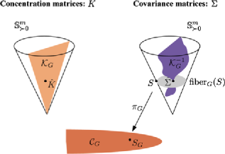
Figure 1: Geometry of maximum likelihood estimation in Gaussian graphical models. The cone $\mathcal{K}_{G}$ consists of all concentration matrices in the model, and $\mathcal{K}_{G}^{-1}$ is the corresponding set of covariance matrices. The cone of sufficient statistics $\mathcal{C}_{G}$ is defined as the projection of $\mathbb{S}^{m}_{\succ 0}$ onto the edge set of $G$. It is dual to $\mathcal{K}_{G}$. Given a sample covariance matrix $S$, $\mathrm{fiber}_{\mathcal{G}}(S)$ consists of all positive definite completions of the $G$-partial matrix $S_{G}$, and it intersects $\mathcal{K}_{G}^{-1}$ in at most one point, namely the MLE $\hat{\Sigma}$.

Theorem 2.2

For a graph $G$ the following statements are equivalent:

A $G$-partial matrix $M_{G}\in\mathbb{R}^{E}$ has a positive definite completion if and only if all submatrices corresponding to maximal cliques in $M_{G}$ are positive definite.

$G$ is chordal.

By combining Theorems 2.1 and 2.2 we get the following result about the existence of the MLE in Gaussian graphical models (see also Buhl ).

Corollary 2.3

If $n\geq q^{*}$, the MLE exists with probability 1. If $n<q$, the MLE does not exist.

Note that chordal graphs have $q^{*}=q$. Therefore, existence of the MLE only depends on the number of observations. For nonchordal graphs, however, there is a gap $q\leq n<q^{*}$, in which existence of the MLE is not well understood. Cycles and wheels (cycles with one additional completely connected vertex) are the only nonchordal graphs, which have been studied Barrett2 , Barrett1 , Buhl . We will extend the results on cycles and wheels to bipartite graphs $K_{2,m}$ and small grids.

3 Geometry of maximum likelihood estimation in Gaussian graphical models

Every concentration matrix (i.e., inverse of a covariance matrix) in a Gaussian graphical model satisfies the undirected pairwise Markov property (1). The set of all concentration matrices in the model is a convex cone

$$\mathcal{K}_{G}:=\{K\in\mathbb{S}^{m}_{\succ 0}\mid K_{ij}=0,\forall(i,j)\notin E\}.$$

Note again that the edge set contains all self-loops, that is, $(i,i)\in E$ for all $i\in[m]$. By taking the inverse of every matrix in $\mathcal{K}_{G}$, we get the set of all covariance matrices in the model denoted by $\mathcal{K}_{G}^{-1}$. This is an algebraic variety intersected with the positive definite cone $\mathbb{S}^{m}_{\succ 0}$ and shown in purple in Figure 1.

In a Gaussian graphical model, the $G$-partial matrix $S_{G}$ is a minimal sufficient statistic of a sample covariance matrix $S$ (e.g., Lauritzen , Whittaker ). So Theorem 2.1 has the following geometric interpretation also explained in Figure 1:

Corollary 3.1

The MLEs $\hat{\Sigma}$ and $\hat{K}$ exist for a given sample covariance matrix $S$ if and only if

$$\mathrm{fiber}_{\mathcal{G}}(S):=\{\Sigma\in\mathbb{S}^{m}_{\succ 0}\mid\Sigma_{G}=S_{G}\}$$

is nonempty, in which case $\mathrm{fiber}_{\mathcal{G}}(S)$ intersects $\mathcal{K}_{G}^{-1}$ in exactly one point, namely the MLE $\hat{\Sigma}$.

So the MLE $\hat{\Sigma}$ has an algebraic description in terms of the sufficient statistic $S_{G}$, that is, $\hat{\Sigma}$ can be represented as a solution to polynomial equations in the sufficient statistic $S_{G}$. The maximal degree of these polynomials is called the ML degree. The ML degree describes the map taking a sample covariance matrix $S$ to its maximum likelihood estimate $\hat{\Sigma}$ and is studied in more detail in Section 4.

Applying Corollary 3.1, we can describe the set of all sufficient statistics for which the MLE exists. We denote this set by $\mathcal{C}_{G}$. It is given by the projection of the positive definite cone $\mathbb{S}^{m}_{\succ 0}$ onto the edge set of the graph $G$:

$$\mathcal{C}_{G}:=\pi_{G}(\mathbb{S}^{m}_{\succ 0}).$$

So $\mathcal{C}_{G}$ is also a convex cone and shown in dark orange in Figure 1. Moreover, we proved in ourpaper , Proposition 2.1, that the cone of sufficient statistics $\mathcal{C}_{G}$ is the convex dual to the cone of concentration matrices $\mathcal{K}_{G}$.

Example 3.2.

For small-dimensional problems we are able to give a graphical representation of the cone of sufficient statistics $\mathcal{C}_{G}$. For example, consider the Gaussian graphical model on the bipartite graph $K_{2,3}$ with concentration matrices of the form

$$K=\pmatrix{\lambda_{1}&0&\lambda_{2}&\lambda_{3}&\lambda_{4}\cr 0&\lambda_{1}&\lambda_{4}&\lambda_{2}&\lambda_{3}\cr\lambda_{2}&\lambda_{4}&\lambda_{1}&0&0\cr\lambda_{3}&\lambda_{2}&0&\lambda_{1}&0\cr\lambda_{4}&\lambda_{3}&0&0&\lambda_{1}},\qquad\raisebox{-27.0pt}{ \includegraphics{957i01.eps} }$$

Note that in order to reduce the number of parameters and be able to draw $\mathcal{C}_{G}$ in three-dimensional space, we assume additional equality constraints on the nonzero entries of the concentration matrix, represented by the graph coloring above. Such colored Gaussian graphical models, where the coloring represents equality constraints on the concentration matrix, are called RCON-models and have been introduced in Hojsgaard .

(a)		(b)
(c)	(d)	(e)

Figure 2: These pictures illustrate the convex geometry of maximum likelihood estimation for Gaussian graphical models. The cone of concentration matrices $\mathcal{K}_{G}$ is shown in (a), its algebraic boundary in (b), the dual cone of sufficient statistics in (c) and its algebraic boundary in (d) and (e), where (d) is the transparent version of (e).

Without loss of generality we can rescale $K$ and assume that all diagonal entries are one. The cone of concentration matrices $\mathcal{K}_{G}$ for this model is shown in Figure 2(a). Its algebraic boundary is described by $\{\operatorname{det}(K)=0\}$ and is shown in Figure 2(b). In this example, the determinant factors into two components, a cylinder and an ellipsoid. Dualizing the boundary of $\mathcal{K}_{G}$ by the algorithm described in our previous paper (ourpaper , Proposition 2.4) results in the hypersurface shown in Figure 2(e). The double cone is dual to the cylinder in Figure 2(b). By making the double cone transparent as shown in Figure 2(d), we see the enclosed ellipsoid, which is dual to the ellipsoid in Figure 2(b). The cone of sufficient statistics $\mathcal{C}_{G}$ is shown in Figure 2(c). The MLE exists if and only if the sufficient statistic lies in the interior of this convex body. Using the elimination criterion of Theorem 3.3, we can show that the MLE exists with probability one already for one observation.

In this paper, we examine the existence of the MLE for $n$ observations in the range $q\leq n<q^{*}$, for which the existence of the MLE is not well understood. Geometrically, we look at the manifold of rank $n$ matrices on the boundary of the cone $\mathbb{S}^{m}_{\succeq 0}$. In general, its projection

$$\pi_{G}\bigl{(}\{M\in\mathbb{S}^{m}_{\succeq 0}\mid\mathrm{rk}(M)=n\}\bigr{)}$$ (2)

lies in the topological closure of the cone $\mathcal{C}_{G}$. The MLE exists with probability one for $n$ observations if and only if the projection (2) lies in the interior of $\mathcal{C}_{G}$.

Based on the geometric interpretation of maximum likelihood estimation in Gaussian graphical models, we can derive a sufficient condition for the existence of the MLE. The following algebraic elimination criterion can be used as an algorithm to establish existence of the MLE with probability one for $n$ observation.

Theorem 3.3 ((Elimination criterion))

Let $I_{G,n}$ be the elimination ideal obtained from the ideal of $(n+1)\times(n+1)$-minors of a symmetric $m\times m$ matrix $S$ of unknowns by eliminating all unknowns corresponding to nonedges of the graph $G$. If $I_{G,n}$ is the zero ideal, then the MLE exists with probability one for $n$ observations.

The variety corresponding to the ideal of $(n+1)\times(n+1)$-minors of a symmetric $m\times m$ matrix $S$ of unknowns consists of all $m\times m$ matrices of rank at most $n$. Eliminating all unknowns corresponding to nonedges of the graph $G$ results in the elimination ideal $I_{G,n}$ (see, e.g., Cox ) and is geometrically equivalent to a projection onto the cone of sufficient statistics $\mathcal{C}_{G}$. Let $V$ be the variety corresponding to the elimination ideal $I_{G,n}$. We denote by $k$ its dimension and by $\mu$ a $k$-dimensional Lebesgue measure. The MLE exists with probability one for $n$ observations if

$$\mu(V\cap\partial\mathcal{C}_{G})=0,$$

where $\partial\mathcal{C}_{G}$ denotes the boundary of the cone of sufficient statistics $\mathcal{C}_{G}$.

If $I_{G,n}$ is the zero ideal, then the variety $V$ is full-dimensional, and its dimension $\dim(V)=k=\dim(\mathcal{C}_{G})$. So if we assume that $\mu(V\cap\partial\mathcal{C}_{G})>0$, then $\mu(\partial\mathcal{C}_{G})>0$, which is a contradiction to $\dim(\partial\mathcal{C}_{G})<k$.

For small examples, the elimination ideal $I_{G,n}$ can be computed, for example, using Macaulay2 Macaulay2 , a software system for research in algebraic geometry. If $I_{G,n}$ is not the zero ideal, then an analysis of polynomial inequalities is required. One needs to carefully examine how the components of $V$ are located. The argument is subtle because the algebraic boundary of $\mathcal{C}_{G}$ may in fact intersect the interior of $\mathcal{C}_{G}$. So even if the projection $V$ is a component of the algebraic boundary of $\mathcal{C}_{G}$, the MLE might still exist with positive probability. We will encounter and describe such an example in detail in Section 6.

4 Bipartite graphs

In this section, we first derive the MLE existence results for bipartite graphs $K_{2,m}$ paralleling the results on cycles proven by Buhl Buhl . Let the graph $K_{2,m}$ be labeled as shown in Figure 3. A minimal chordal cover is given in Figure 3 (right). As for cycles, for bipartite graphs $K_{2,m}$ we have $q=2$ and $q^{*}=3$. Therefore only the case of $n=2$ observations is interesting.

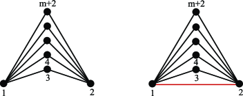
Figure 3: Bipartite graph $K_{2,m}$ (left) and minimal chordal cover of $K_{2,m}$ (right).

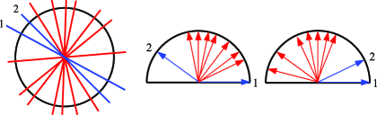
Figure 4: The MLE on $K_{2,m}$ exists in the following situations. Lines and data vectors corresponding to the variables 1 and 2 are drawn in blue. Lines and data vectors corresponding to the variables $3,4,\ldots,m+2$ are drawn in red.

Let $X_{1}$ and $X_{2}$ denote two independent samples from the distribution $\mathcal{N}_{m+2}(0$, $\Sigma)$, which obeys the undirected pairwise Markov property on $K_{2,m}$. We denote by $X$ the $(m+2)\times 2$ data matrix consisting of the two samples $X_{1}$ and $X_{2}$ as columns. The rows of $X$ are denoted by $x_{1},\ldots,x_{m+2}$. Similarly as for cycles in Buhl , we will describe a criterion on the configuration of data vectors $x_{1},\ldots,x_{m+2}$ ensuring the existence of the MLE. Our proof is essentially the same argument as used by Buhl Buhl for cycles. The following characterization of positive definite matrices of size $3\times 3$ proven in Barrett1 will be helpful in this context.

Lemma 4.1

The matrix

$$\pmatrix{1&\cos(\alpha)&\cos(\beta)\cr\cos(\alpha)&1&\cos(\gamma)\cr\cos(\beta)&\cos(\gamma)&1}$$

with $0<\alpha,\beta,\gamma<\pi$ is positive definite if and only if

$$\alpha<\beta+\gamma,\qquad\beta<\alpha+\gamma,\qquad\gamma<\alpha+\beta,\qquad\alpha+\beta+\gamma<2\pi.$$

Proposition 4.2

The MLE on the graph $K_{2,m}$ exists with probability one for $n\geq 3$ observations, and the MLE does not exist for $n<2$ observations. For $n=2$ observations the MLE exists if and only if the lines generated by $x_{1}$ and $x_{2}$ are direct neighbors [see Figure 4 (left)].

Because the problem of existence of the MLE is a positive definite matrix completion problem, we can rescale and rotate the data vectors $x_{1},\ldots,x_{m+2}$ (i.e., perform an orthogonal transformation) without changing the problem. So without loss of generality we can assume that the vectors $x_{1},\ldots,x_{m+2}\in\mathbb{R}^{2}$ have length one, lie in the upper unit half circle and $x_{1}=(1,0)$. We need to prove that the MLE exists if and only if the data configuration is as shown in Figure 4 (middle) or (right).

Let $\theta_{ij}$ denote the angle between vector $x_{i}$ and $x_{j}$. Then the $K_{2,m}$-partial sample covariance matrix $S_{K_{2,m}}$ is of the form

$$\left(\begin{tabular}[]{cc|cccc}1&$\star$&$\cos(\theta_{13})$&$\cos(\theta_{14})$&$\cdots$&$\cos(\theta_{1,m+2})$\\ $\star$&1&$\cos(\theta_{23})$&$\cos(\theta_{24})$&$\cdots$&$\cos(\theta_{2,m+2})$\\ \hline\cr$\cos(\theta_{13})$&$\cos(\theta_{23})$&1&$\star$&$\cdots$&$\star$\\ $\cos(\theta_{14})$&$\cos(\theta_{24})$&$\star$&1&$\ddots$&$\vdots$\\ $\vdots$&$\vdots$&$\vdots$&$\ddots$&$\ddots$&$\star$\\ $\cos(\theta_{1,m+2})$&$\cos(\theta_{2,m+2})$&$\star$&$\cdots$&$\star$&1\\ \end{tabular}\right).$$

We put stars ($\star$) at all positions not corresponding to edges in the graph. The stars represent the entries of the sample covariance matrix which are not part of the sufficient statistics.

The graph $K_{2,m}$ can be extended to a chordal graph by adding one edge as shown in Figure 3 (right). So by Theorem 2.2, $S_{K_{2,m}}$ can be extended to a positive definite matrix if and only if the $(1,2)$ entry of $S_{K_{2,m}}$ can be completed in such a way that all the submatrices corresponding to maximal cliques are positive definite. This is equivalent to the existence of $\rho\in\mathbb{R}$ with $0<\rho<\pi$ such that

$$\pmatrix{1&\cos(\rho)&\cos(\theta_{1i})\cr\cos(\rho)&1&\cos(\theta_{2i})\cr\cos(\theta_{1i})&\cos(\theta_{2i})&1}\succ 0\qquad\mbox{for all }i\in\{3,4,\ldots,m+2\}.$$

By Lemma 4.1 this occurs if and only if

$$\left.\matrix{\theta_{1i}-\theta_{2i}\cr\theta_{2i}-\theta_{1i}}\right\}<\rho<\left\{\matrix{\theta_{1j}+\theta_{2j}\cr 2\pi-\theta_{1j}-\theta_{2j}}\right.\qquad\mbox{for all }i,j\in\{3,4,\ldots,m+2\},$$

which is equivalent to

$$2\theta_{ai}<\theta_{1i}+\theta_{2i}+\theta_{1j}+\theta_{2j}<2\pi+2\theta_{ai}$$ (3)

for all $a\in\{1,2\}$, $i,j\in\{3,4,\ldots,m+2\}$. We distinguish two cases. [Case 2.]

There is a vector $x_{j}$ lying between $x_{1}$ and $x_{2}$, which implies that $\theta_{1j}+\theta_{2j}=\theta_{12}$. If there was a vector $x_{i}$, $i\neq j$, which does not lie between $x_{1}$ and $x_{2}$, then

$$\theta_{1j}+\theta_{2j}+\theta_{1i}+\theta_{2i}=2\theta_{1i},$$

which is a contradiction to (3). Hence all vectors $x_{3},x_{4},\ldots x_{m+2}$ lie between $x_{1}$ and $x_{2}$, in which case

$$\theta_{1i}+\theta_{2i}+\theta_{1j}+\theta_{2j}=2\theta_{12},$$

and inequality (3) is satisfied.

The vectors $x_{1}$ and $x_{2}$ are direct neighbors, which implies that $\theta_{1i}+\theta_{2i}=\theta_{12}+2\theta_{2i}$ for all $i\in\{3,4,\ldots,m+2\}$, in which case inequality (3) is satisfied.

This proves that for two observations, the MLE exists if and only if the data configuration is as shown in Figure 4 (middle) or (right).

The geometric explanation of what is happening in this example is that the projection of the positive definite matrices of rank 2 intersects the interior and the boundary of the cone of sufficient statistics $\mathcal{C}_{G}$ with positive measure. The sufficient statistics originating from data vectors, where lines 1 and 2 are neighbors, lie in the interior of $\mathcal{C}_{G}$. If lines 1 and 2 are not neighbors, the corresponding sufficient statistics lie on the boundary of the cone $\mathcal{C}_{G}$, and the MLE does not exist. A similar situation is encountered in Example 6.2 and depicted in Figure 8.

It is worth remarking that if the $m+2$ variables are independent, we can compute the probability of existence of the MLE by a combinatorial argument. In this case, the probability that the MLE exists is given by

$$\frac{2m!}{(m+1)!}=\frac{2}{m+1}.$$

A different approach to gaining a better understanding of maximum likelihood estimation in Gaussian graphical models is to study the ML degree of the underlying graph. The map taking a sample covariance matrix $S$ to its maximum likelihood estimate $\hat{\Sigma}$ is an algebraic function, and its degree is the ML degree of the model. See Oberwolfach , Definition 2.1.4. The ML degree represents the algebraic complexity of the problem of finding the MLE. This suggests that a larger ML degree results in a more difficult MLE existence problem. We proved in ourpaper that the ML degree is one if and only if the underlying graph is chordal. It is conjectured in Oberwolfach , Section 7.4, that the ML degree of the cycle grows exponentially in the cycle length. An interesting contrast to the cycle conjecture is the following theorem, where we prove that the ML degree for bipartite graphs $K_{2,m}$ grows linearly in the number of variables.

Theorem 4.3

In a Gaussian graphical model with underlying graph $K_{2,m}$ the ML degree is $2m+1$.

Given a generic matrix $S\in\mathbb{S}^{m+2}$, we fix $\Sigma\in\mathbb{S}^{m+2}$ with entries $\Sigma_{ij}=S_{ij}$ for $(i,j)\in E$ and unknowns $\Sigma_{12}=\Sigma_{21}=y$ and $\Sigma_{ij}=z_{ij}$ for all other $(i,j)\notin E$. We denote by $K=\Sigma^{-1}$ the corresponding concentration matrix. The ML degree of $K_{2,m}$ is the number of complex solutions to

$$(\Sigma^{-1})_{ij}=0\qquad\mbox{for all }(i,j)\notin E.$$

Let $A$ denote the set consisting of the two distinguished vertices $\{1,2\}$, and let $B=V\setminus A$. In the following we will use the block structure

$$\Sigma=\pmatrix{\Sigma_{AA}&\Sigma_{AB}\cr\Sigma_{BA}&\Sigma_{BB}},\qquad K=\pmatrix{K_{AA}&K_{AB}\cr K_{BA}&K_{BB}}.$$

For example, for the graph $K_{2,5}$ the corresponding covariance matrix $\Sigma$ and concentration matrix $K$ are of the form

S13S231z34z35S14S24z341z45S15S25z35z451),fragments fragments fragmentsS13fragmentsS231fragmentsz34fragmentsz35fragmentsS14fragmentsS24fragmentsz341fragmentsz45fragmentsS15fragmentsS25fragmentsz35fragmentsz451\displaystyle\left(\begin{tabular}[]{cc|ccc}1&$y$&$S_{13}$&$S_{14}$&$S_{15}$\\ $y$&$1$&$S_{23}$&$S_{24}$&$S_{25}$\\ \hline\cr$S_{13}$&$S_{23}$&1&$z_{34}$&$z_{35}$\\ $S_{14}$&$S_{24}$&$z_{34}$&1&$z_{45}$\\ $S_{15}$&$S_{25}$&$z_{35}$&$z_{45}$&1\end{tabular}\right), K13K23K3300K14K240K440K15K2500K55).fragments fragments fragmentsK13fragmentsK23fragmentsK3300fragmentsK14fragmentsK240fragmentsK440fragmentsK15fragmentsK2500fragmentsK55\displaystyle\left(\begin{tabular}[]{cc|ccc}$K_{11}$&$0$&$K_{13}$&$K_{14}$&$K_{15}$\\ 0&$K_{22}$&$K_{23}$&$K_{24}$&$K_{25}$\\ \hline\cr$K_{13}$&$K_{23}$&$K_{33}$&0&0\\ $K_{14}$&$K_{24}$&0&$K_{44}$&0\\ $K_{15}$&$K_{25}$&0&0&$K_{55}$\end{tabular}\right).

$$\Sigma = \left(\begin{tabular}[]{cc|ccc}1&$y$&$S_{13}$&$S_{14}$&$S_{15}$\\ $y$&$1$&$S_{23}$&$S_{24}$&$S_{25}$\\ \hline\cr$S_{13}$&$S_{23}$&1&$z_{34}$&$z_{35}$\\ $S_{14}$&$S_{24}$&$z_{34}$&1&$z_{45}$\\ $S_{15}$&$S_{25}$&$z_{35}$&$z_{45}$&1\end{tabular}\right),$$ 1yS13S14S15y1S23S24S251yS13S14S15y1S23S24S25

$$K = \left(\begin{tabular}[]{cc|ccc}$K_{11}$&$0$&$K_{13}$&$K_{14}$&$K_{15}$\\ 0&$K_{22}$&$K_{23}$&$K_{24}$&$K_{25}$\\ \hline\cr$K_{13}$&$K_{23}$&$K_{33}$&0&0\\ $K_{14}$&$K_{24}$&0&$K_{44}$&0\\ $K_{15}$&$K_{25}$&0&0&$K_{55}$\end{tabular}\right).$$ K110K13K14K150K22K23K24K25K110K13K14K150K22K23K24K25

Note that the block $K_{BB}$ is a diagonal matrix. Hence the Schur complement

$$\Sigma_{BB}-\Sigma_{BA}\Sigma_{AA}^{-1}\Sigma_{AB}$$

is also a diagonal matrix. Writing out the off-diagonal entries of this matrix results in the following expression for the variables $z$ in terms of the variable $y$:

$$z_{ij}=-\frac{1}{1-y^{2}}\bigl{(}y(S_{1i}S_{2j}+S_{1j}S_{2i})-S_{1i}S_{1j}-S_{2i}S_{2j}\bigr{)}.$$

Setting the minor $M_{12}$ of $\Sigma$ to zero results in the last equation of the form

$$y\det(\Sigma_{BB})+(\mbox{polynomial in $z$ of degree $m-1$})=0.$$ (6)

We note that $\det(\Sigma_{BB})$ is a polynomial in $z$ of degree $m$, where the degree 0 term is 1. So by multiplying equation (6) with $(1-y^{2})^{m}$, we get a degree $2m+1$ equation in y and therefore $2m+1$ complex solutions for $y$. For each solution of $y$ we get one solution for the variables $z$, which proves that the ML degree of $K_{2,m}$ is $2m+1$.

Bipartite graphs and cycles are classes of graphs with $q=2$ and $q^{*}=3$. What can we say about such graphs in general regarding the existence of the MLE for two observations? A related question has been studied from a purely algebraic point of view in Barrett2 . A cycle-completable graph is defined to be a graph such that every partial matrix $M_{G}$ has a positive definite completion if and only if $M_{G}$ is positive definite on all submatrices corresponding to maximal cliques in the graph, and all submatrices corresponding to cycles in the graph can be completed to a positive definite matrix. It is shown in Barrett2 that a graph is cycle-completable if and only if there is a chordal cover with no new 4-clique.

Buhl Buhl studied cycles from a more statistical point of view and described a criterion on the data vectors for the existence of the MLE for two observations. Combining the results of Barrett2 and Buhl , we get the following result:

Corollary 4.4

Let $G$ be a graph with $q=2$ and $q^{*}\geq 3$. Then the following statements are equivalent:

For $n=2$ observations, the MLE exists if and only if Buhl’s cycle condition is satisfied on every induced cycle.

$q^{*}=3$.

This result solves the problem of existence of the MLE for all graphs with $q=2$ and $q^{*}=3$. Note that Corollary 4.4 is more general than Proposition 4.2. The proof, however, is more involved and less constructive.

For bipartite graphs $K_{3,m}$ the situation is more complicated and we do not yet have results similar to Proposition 4.2 and Theorem 4.3. We will nevertheless describe some preliminary results.

Figure 5: Bipartite graph $K_{3,m}$ (left) and minimal chordal cover of $K_{3,m}$ (middle). The tetrahedron-shaped pillow consisting of all positive semidefinite $3\times 3$ matrices with ones on the diagonal is shown in the right figure.

Let the graph $K_{3,m}$ be labeled as shown in Figure 5. A minimal chordal cover is given in Figure 5 (middle). Hence, $q=2$ and $q^{*}=4$. The convex body shown in Figure 5 (right) consists of all positive semidefinite $3\times 3$ matrices with ones on the diagonal. We call it the tetrahedron-shaped pillow. We will prove that the existence of the MLE is equivalent to a nonempty intersection of such inflated and shifted tetrahedron-shaped pillows.

Corollary 4.5

The MLE on the graph $K_{3,m}$ exists if and only if the $m$ inflated and shifted tetrahedron-shaped pillows corresponding to the maximal cliques in a minimal chordal cover of $K_{3,m}$ shown in Figure 5 (middle) have nonempty intersections.

Applying Theorem 2.2 in a similar way as in the proof of Theorem 4.2, the partial covariance matrix $S_{K_{3,m}}$ can be extended to a positive definite matrix if and only if the entries corresponding to the missing edges $(1,2)$, $(1,3)$ and $(2,3)$ can be completed in such a way that all the submatrices corresponding to maximal cliques in the minimal chordal cover (Figure 5, middle) are positive definite. This is equivalent to the existence of $x,y,z\in\mathbb{R}$ with $-1<x,y,z<1$ such that

$$\pmatrix{1&s_{1i}&s_{2i}&s_{3i}\cr s_{1i}&1&x&y\cr s_{2i}&x&1&z\cr s_{3i}&y&z&1}\succ 0\qquad\mbox{for all }i\in\{4,5,\ldots,m+3\},$$ (7)

where $s_{ai}$, $a\in\{1,2,3\}$, $i\in\{4,5,\ldots,m+3\}$ are the sufficient statistics corresponding to edges in the bipartite graph $K_{3,m}$. Using Schur complements and rescaling, (7) holds if and only if

$$\pmatrix{1&x_{i}&y_{i}\cr x_{i}&1&z_{i}\cr y_{i}&z_{i}&1}\succ 0\qquad\mbox{for all }i\in\{4,5,\ldots,m+3\},$$ (8)

where

$$x_{i} = \frac{x-s_{1i}s_{2i}}{\sqrt{1-s_{1i}^{2}}\sqrt{1-s_{2i}^{2}}},\qquad y_{i}=\frac{y-s_{1i}s_{3i}}{\sqrt{1-s_{1i}^{2}}\sqrt{1-s_{3i}^{2}}},$$

$$z_{i} = \frac{x-s_{2i}s_{3i}}{\sqrt{1-s_{2i}^{2}}\sqrt{1-s_{3i}^{2}}}.$$

So the MLE exists if and only if the inflated and shifted tetrahedron-shaped pillows corresponding to the inequalities in (8) have nonempty intersection.

We used the software package Macaulay2 to compute the ML degree of $K_{3,m}$ for $m\leq 4$. It is an open problem to find a general formula or a recurrence relation for the ML degree of $K_{l,m}$, where $l\geq 3$.

$m$	1	2	3	4
ML degree	1	7	57	131

5 Small graphs

In this section we analyze the $3\times 3$ grid in particular and complete the discussion of ourpaper with the number of observations and the corresponding existence probability of the MLE for all graphs with 5 or less vertices.

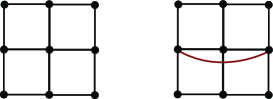
Figure 6: $3\times 3$ grid $\mathcal{H}$ (left) and grid with additional edge $\mathcal{H}^{\prime}$ (right).

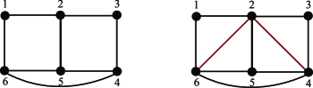
Figure 7: Graph $\mathcal{G}$ (left) and minimal chordal cover of $\mathcal{G}$ (right).

The $3\times 3$ grid is shown in Figure 6 (left) and has $q=2$ and $q^{*}=4$. This example represents the starting point of this paper and is the original problem posed by Steffen Lauritzen during his lecture at the “Durham Symposium on Mathematical Aspects of Graphical Models” in 2008. As a preparation, we first discuss the existence of the MLE for the graph $\mathcal{G}$ on six vertices shown in Figure 7. The graph $\mathcal{G}$ also has $q=2$ and $q^{*}=4$, and is the first example for which we can prove that the bound $n\geq q^{*}$ for the existence of the MLE with probability one is not tight and that the MLE can exist with probability one, even when the number of observations equals the treewidth.

Theorem 5.1

The MLE on the graph $\mathcal{G}$ (Figure 7, left) exists with probability one for $n=3$ observations.

We compute the ideal $I_{\mathcal{G},3}$ by eliminating the variables $s_{13},s_{15},\allowbreak s_{16}$, $s_{24},s_{26},s_{34},s_{35}$ from the ideal of $4\times 4$ minors of the matrix $S$ given in (9). This results in the zero ideal, which by Theorem 3.3 completes the proof.

Remark 5.2.

Theorem 5.1 is equivalent to the following purely algebraic statement. Let

$$S=\pmatrix{1&s_{12}&s_{13}&s_{14}&s_{15}&s_{16}\cr s_{12}&1&s_{23}&s_{24}&s_{25}&s_{26}\cr s_{13}&s_{23}&1&s_{34}&s_{35}&s_{36}\cr s_{14}&s_{24}&s_{34}&1&s_{45}&s_{46}\cr s_{15}&s_{25}&s_{35}&s_{45}&1&s_{56}\cr s_{16}&s_{26}&s_{36}&s_{46}&s_{56}&1}\in\mathbb{S}^{6}_{\succeq 0}$$ (9)

with $\operatorname{rank}(S)=3$. Then there exist $x,y,a,b,c,d,e\in\mathbb{R}$ such that

$$S^{\prime}=\pmatrix{1&s_{12}&a&s_{14}&b&c\cr s_{12}&1&s_{23}&x&s_{25}&y\cr a&s_{23}&1&d&e&s_{36}\cr s_{14}&x&d&1&s_{45}&s_{46}\cr b&s_{25}&e&s_{45}&1&s_{56}\cr c&y&s_{36}&s_{46}&s_{56}&1}\in\mathbb{S}^{6}_{\succ 0}.$$

So any partial matrix of rank 3 with specified entries at all positions corresponding to edges in $\mathcal{G}$ can be completed to a positive definite matrix.

Corollary 5.3

Let $\mathcal{H}$ be the $3\times 3$-grid shown in Figure 6. Then the MLE on $\mathcal{H}$ exists with probability one for $n\geq 3$ observations, and the MLE does not exist for $n<2$ observations.

First note that Groebner bases computations are extremely memory intensive and the elimination ideal $I_{\mathcal{H},3}$ cannot be computed directly due to insufficient memory. We solve this problem by gluing together smaller graphs. The probability of existence of the MLE for the $3\times 3$ grid $\mathcal{H}$ is at least as large as the existence probability when the underlying graph is $\mathcal{H}^{\prime}$. The graph $\mathcal{H}^{\prime}$ is a clique sum of two graphs of the form $\mathcal{G}$, for which the MLE existence probability is one for $n\geq 3$.

This example shows that although we are not able to compute the elimination ideal for large graphs directly, the algebraic elimination criterion (Theorem 3.3) is still useful also in this situation. We can study small graphs with the elimination criterion and glue them together using clique sums to build larger graphs.

For two observations on the $3\times 3$ grid, the cycle conditions are necessary but not sufficient for the existence of the MLE (Corollary 4.4). Unlike for bipartite graphs $K_{2,m}$, the existence of the MLE does not only depend on the ordering of the lines corresponding to the data vectors in $\mathbb{R}^{2}$. By simulations with the Matlab software cvx CVX , one can easily find orderings for which the MLE sometimes exists and sometimes does not. Finding a necessary and sufficient criterion for the existence of the MLE for two observations remains an open problem.

=280pt Graph $\bolds{G}$ 1 obs. 2 obs. 3 obs. $\bolds{\geq}$4 obs. (a) No $p\in(0,1)$ $p=1$ $p=1$ (b) No $p\in(0,1)$ $p=1$ $p=1$ (c) No $p\in(0,1)$ $p=1$ $p=1$ (d) No No $p=1$ $p=1$ (e) No $p\in(0,1)$ $p=1$ $p=1$ (f) No No $p=1$ $p=1$ (g) No No $p\in(0,1)$ $p=1$

Table 1: This table shows the number of observations (obs.) and the corresponding MLE existence probability for all nonchordal graphs on 5 or fewer vertices

We now complete the discussion of ourpaper with the number of observations and the corresponding existence probability of the MLE for all graphs with 5 or less vertices. All nonchordal graphs with 5 or less vertices are shown in Table 1. The 4-cycle and 5-cycle in (a) and (b) are covered by Buhl’s results Buhl . The graphs in (c) and (d) are clique sums of two graphs and therefore completable if and only if the submatrices corresponding to the two subgraphs are completable. Graph (e) is the bipartite graph $K_{2,3}$ and covered by Theorem 4.2. For the graph in (f) $q=3$ and $q^{*}=4$. Applying the elimination criterion from Theorem 3.3 shows that three observations are sufficient for the existence of the MLE. The last example, the 5-wheel in graph (g), is also covered by Buhl’s results Buhl .

6 Colored Gaussian graphical models

For some applications, symmetries in the underlying Gaussian graphical model can be assumed. Adding symmetry to the conditional independence restrictions of a graphical model reduces the number of parameters and in some cases also the number of observations needed for the existence of the MLE. The symmetry restrictions can be represented by a graph coloring, where edges, or vertices, respectively, have the same coloring if the corresponding elements of the concentration matrix are equal. Such models are called RCON-models Hojsgaard . We discussed such a model earlier in Example 3.2.

We denote the uncolored graph by $G$ and the colored graph by $\mathcal{G}$. Note that in this section the graph $G$ does not contain any self-loops. Let the vertices be colored with $p$ different colors and the edges with $q$ different colors:

$$V = V_{1}\sqcup V_{2}\sqcup\cdots\sqcup V_{p},\qquad p\leq|V|,$$

$$E = E_{1}\sqcup E_{2}\sqcup\cdots\sqcup E_{q},\qquad q\leq|E|.$$

Then the set of all concentration matrices $\mathcal{K}_{\mathcal{G}}$ consists of all positive definite matrices satisfying:

• $K_{\alpha\beta}=0$ for any pair of vertices $\alpha,\beta$ that do not form an edge in $G$.

• $K_{\alpha\alpha}=K_{\beta\beta}$ for any pair of vertices $\alpha,\beta$ in a common vertex color class $V_{i}$.

• $K_{\alpha\beta}=K_{\gamma\delta}$ for any pair of edges $(\alpha,\beta),(\gamma,\delta)$ in a common edge color class $E_{j}$.

This means that also for RCON-models the set $\mathcal{K}_{\mathcal{G}}$ is defined by linear equations on the concentration matrix $K$. So the geometry of maximum likelihood estimation is the same as that explained in Section 3, and it is straightforward to derive the equivalent of Theorem 2.1 for colored Gaussian graphical models.

Theorem 6.1

In a colored Gaussian graphical model on $\mathcal{G}$ the MLE of the covariance matrix $\Sigma$ exists if and only if there is a positive definite matrix $\tilde{\Sigma}$ such that

$$\sum_{\alpha\in V_{i}}\tilde{\Sigma}_{\alpha\alpha}=\sum_{\alpha\in V_{i}}S_{\alpha\alpha}\quad\mbox{and}\quad\sum_{(\alpha,\beta)\in E_{j}}\tilde{\Sigma}_{\alpha\beta}=\sum_{(\alpha,\beta)\in E_{j}}S_{\alpha\beta}$$

for all vertex color classes $V_{1},\ldots,V_{p}$ and all edge color classes $E_{1},\ldots,E_{q}$. Then the MLE $\hat{\Sigma}$ is the unique completion with $(\hat{\Sigma}^{-1})_{\alpha\alpha}=(\hat{\Sigma}^{-1})_{\beta\beta}$ for any pair of vertices $\alpha,\beta$ in a common vertex color class $V_{i}$, $(\hat{\Sigma}^{-1})_{\alpha\beta}=(\hat{\Sigma}^{-1})_{\gamma\delta}$ for any pair of edges $(\alpha,\beta),(\gamma,\delta)$ in a common edge color class $E_{j}$, and $(\hat{\Sigma}^{-1})_{\alpha\beta}=0$ for all $(\alpha,\beta)\notin E$.

Example 6.2 ((Frets’s heads)).

We revisit the heredity study of head dimensions known as Frets’s heads reported in Frets . Part of the original data are the length and breadth of the heads of 25 pairs of first and second sons. This data set was also discussed in MKB , ourpaper . The data supports the following colored Gaussian graphical model, where the joint distribution remains the same when the two sons are exchanged:

$$K=\pmatrix{\lambda_{1}&\lambda_{3}&0&\lambda_{4}\cr\lambda_{3}&\lambda_{1}&\lambda_{4}&0\cr 0&\lambda_{4}&\lambda_{2}&\lambda_{5}\cr\lambda_{4}&0&\lambda_{5}&\lambda_{2}},\qquad\raisebox{-19.0pt}{ \includegraphics{957i09.eps} }$$

In this graph, variable 1 corresponds to the length of the first son’s head, variable 2 to the length of the second son’s head, variable 3 to the breadth of the second son’s head and variable 4 to the breadth of the first son’s head. Color classes consisting only of one edge (or vertex) are displayed in black.

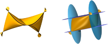
Figure 8: All possible sufficient statistics from one observation are shown on the left. The cone of sufficient statistics is shown on the right.

Given a sample covariance matrix $S=(s_{ij})$, the five sufficient statistics for this model according to the graph coloring are

$$t_{1} = s_{11}+s_{22},\qquad t_{2}=s_{33}+s_{44},\qquad t_{3}=2s_{12},$$

$$t_{4} = 2(s_{23}+s_{14}),\qquad t_{5}=2s_{34}.$$

The algebraic boundary of the cone of sufficient statistics $\mathcal{C}_{\mathcal{G}}$ is computed in ourpaper and given by the polynomial

$$H_{\mathcal{G}} = (t_{1}-t_{3})\cdot(t_{1}+t_{3})\cdot(t_{2}-t_{5})\cdot(t_{2}+t_{5})$$

$${}\times(4t_{2}^{2}t_{3}^{2}-4t_{1}t_{2}t_{4}^{2}+t_{4}^{4}+8t_{1}t_{2}t_{3}t_{5}-4t_{3}t_{4}^{2}t_{5}+4t_{1}^{2}t_{5}^{2}).$$

For two observations the elimination ideal $I_{\mathcal{G},2}$ is the zero ideal. Therefore, the MLE exists with probability 1 for two or more observations in this model. For one observation we get

$$I_{\mathcal{G},1}=\langle 4t_{2}^{2}t_{3}^{2}-4t_{1}t_{2}t_{4}^{2}+t_{4}^{4}+8t_{1}t_{2}t_{3}t_{5}-4t_{3}t_{4}^{2}t_{5}+4t_{1}^{2}t_{5}^{2}\rangle,$$

which corresponds to one of the components of the algebraic boundary of the cone of sufficient statistics. In this example, the algebraic boundary of the cone of sufficient statistics intersects its interior. This is illustrated in Figure 8. In order to get a graphical representation in three-dimensional space, we fixed $t_{3}$ and $t_{5}$. The variety corresponding to $I_{\mathcal{G},1}$ is shown on the left. We call this hypersurface the bow tie. The cone of sufficient statistics $\mathcal{C}_{\mathcal{G}}$ is the convex hull of the bow tie and shown in Figure 8 (right). Its boundary consists of four planes corresponding to the components $t_{1}-t_{3}$, $t_{1}+t_{3}$, $t_{2}-t_{5}$ and $t_{2}+t_{5}$ shown in blue, and the bows of the bow tie shown in yellow. The black curves show where the planes touch the bow tie. Note that the upper and lower two triangles of the bow tie lie in the interior of $\mathcal{C}_{\mathcal{G}}$. Only the two bows are part of the boundary of $\mathcal{C}_{\mathcal{G}}$. So the MLE exists if the sufficient statistic lies on one of the triangles of the bow tie, and it does not exist if the sufficient statistic lies on one of the bows of the bow tie. Consequently, for one observation the MLE exists with probability strictly between 0 and 1.

A different approach is to run simulations, for example, using cvx. We can generate vectors of length four and compute the MLE by solving a convex optimization problem. If cvx finds a solution, the MLE exists. For this example, however, cvx sometimes does not find a solution, which supports the hypothesis that the MLE exists with probability strictly between 0 and 1 for one observation. In the following, we give a formal proof by characterizing the set of vectors in $\mathbb{R}^{4}$ for which the MLE exists/does not exist.

For this example, we can exactly characterize not just the sufficient statistics, but also the observations, for which the MLE exists. In other words, we can characterize the observations whose sufficient statistics lie on the triangles of the bow tie. First, note that by exchanging variables 1 and 2 and simultaneously exchanging variables 3 and 4, we get the same model. This means that from one observation $X_{1}=(x_{1},x_{2},x_{3},x_{4})$ we can generate a second observation $X_{2}=(x_{2},x_{1},x_{4},x_{3})$. So the resulting data matrix is given by

$$X=\pmatrix{x_{1}&x_{2}\cr x_{2}&x_{1}\cr x_{3}&x_{4}\cr x_{4}&x_{3}}.$$

Applying Buhl’s result about two observations on a Gaussian cycle Buhl , the MLE exists if and only if the lines corresponding to the vectors

$$y_{1}=\pmatrix{x_{1}\cr x_{2}},\qquad y_{2}=\pmatrix{x_{2}\cr x_{1}},\qquad y_{3}=\pmatrix{x_{3}\cr x_{4}},\qquad y_{4}=\pmatrix{x_{4}\cr x_{3}}$$

are not graph consecutive. This is the case if and only if

$$|x_{1}|>|x_{2}|\mbox{ and }|x_{3}|>|x_{4}|\quad\mbox{or}\quad|x_{1}|<|x_{2}|\mbox{ and }|x_{3}|<|x_{4}|.$$ (10)

Hence, the MLE for one observation exists if and only if the data is inconsistent, meaning that the head of the first (second) son is longer than the head of the second (first) son, but the breadth is smaller. In this situation the corresponding sufficient statistics lie on the triangles of the bow tie in Figure 8. Otherwise the corresponding sufficient statistics lie on the bows of the bow tie. If $\Sigma$ is diagonal, the MLE exists with probability 0.5, since all configurations in (10) have the same probability.

In our previous paper ourpaper we found the defining polynomial $\mathcal{H}_{\mathcal{G}}$ of the cone of sufficient statistics for all colored Gaussian graphical models on the 4-cycle, which have the property that edges in the same color class connect the same vertex color classes. Such models have been studied in Hojsgaard and are of special interest, because they are invariant under rescaling of variables in the same vertex color class. In Tables 2 and 3, we complete the discussion of ourpaper with the number of observations and the corresponding existence probability of the MLE.

=280pt Graph $\bolds{K}$ 1 obs. 2 obs. $\bolds{\geq}$3 obs. (1) $\pmatrix{\lambda_{1}&\lambda_{2}&0&\lambda_{2}\cr\lambda_{2}&\lambda_{1}&\lambda_{3}&0\cr 0&\lambda_{3}&\lambda_{1}&\lambda_{2}\cr\lambda_{2}&0&\lambda_{2}&\lambda_{1}}$ $p=1$ $p=1$ $p=1$ (2) $\pmatrix{\lambda_{1}&\lambda_{3}&0&\lambda_{3}\cr\lambda_{3}&\lambda_{2}&\lambda_{4}&0\cr 0&\lambda_{4}&\lambda_{1}&\lambda_{3}\cr\lambda_{3}&0&\lambda_{3}&\lambda_{2}}$ $p=1$ $p=1$ $p=1$ (3) $\pmatrix{\lambda_{1}&\lambda_{2}&0&\lambda_{2}\cr\lambda_{2}&\lambda_{1}&\lambda_{3}&0\cr 0&\lambda_{3}&\lambda_{1}&\lambda_{3}\cr\lambda_{2}&0&\lambda_{3}&\lambda_{1}}$ $p=1$ $p=1$ $p=1$ (4) $\pmatrix{\lambda_{1}&\lambda_{3}&0&\lambda_{3}\cr\lambda_{3}&\lambda_{1}&\lambda_{4}&0\cr 0&\lambda_{4}&\lambda_{2}&\lambda_{4}\cr\lambda_{3}&0&\lambda_{4}&\lambda_{1}}$ $p=1$ $p=1$ $p=1$ (5) $\pmatrix{\lambda_{1}&\lambda_{3}&0&\lambda_{3}\cr\lambda_{3}&\lambda_{2}&\lambda_{4}&0\cr 0&\lambda_{4}&\lambda_{1}&\lambda_{4}\cr\lambda_{3}&0&\lambda_{4}&\lambda_{2}}$ $p=1$ $p=1$ $p=1$ (6) $\pmatrix{\lambda_{1}&\lambda_{2}&0&\lambda_{2}\cr\lambda_{2}&\lambda_{1}&\lambda_{3}&0\cr 0&\lambda_{3}&\lambda_{1}&\lambda_{4}\cr\lambda_{2}&0&\lambda_{4}&\lambda_{1}}$ $p=1$ $p=1$ $p=1$ (7) $\pmatrix{\lambda_{1}&\lambda_{3}&0&\lambda_{3}\cr\lambda_{3}&\lambda_{1}&\lambda_{4}&0\cr 0&\lambda_{4}&\lambda_{2}&\lambda_{5}\cr\lambda_{3}&0&\lambda_{5}&\lambda_{1}}$ $p\in(0,1)$ $p=1$ $p=1$ (8) $\pmatrix{\lambda_{1}&\lambda_{3}&0&\lambda_{3}\cr\lambda_{3}&\lambda_{2}&\lambda_{4}&0\cr 0&\lambda_{4}&\lambda_{1}&\lambda_{5}\cr\lambda_{3}&0&\lambda_{5}&\lambda_{2}}$ $p\in(0,1)$ $p=1$ $p=1$ (9) $\pmatrix{\lambda_{1}&\lambda_{4}&0&\lambda_{4}\cr\lambda_{4}&\lambda_{2}&\lambda_{5}&0\cr 0&\lambda_{5}&\lambda_{3}&\lambda_{6}\cr\lambda_{4}&0&\lambda_{6}&\lambda_{2}}$ No? $p=1$ $p=1$

Table 2: Results on the number of observations and the MLE existence probability for all colored Gaussian graphical models with some symmetry restrictions (namely, edges in the same color class connect the same vertex color classes) on the 4-cycle

=280pt Graph $\bolds{K}$ 1 obs. 2 obs. $\bolds{\geq}$3 obs. (10) $\pmatrix{\lambda_{1}&\lambda_{2}&0&\lambda_{3}\cr\lambda_{2}&\lambda_{1}&\lambda_{3}&0\cr 0&\lambda_{3}&\lambda_{1}&\lambda_{4}\cr\lambda_{3}&0&\lambda_{4}&\lambda_{1}}$ $p=1$ $p=1$ $p=1$ (11) $\pmatrix{\lambda_{1}&\lambda_{3}&0&\lambda_{4}\cr\lambda_{3}&\lambda_{2}&\lambda_{4}&0\cr 0&\lambda_{4}&\lambda_{1}&\lambda_{5}\cr\lambda_{4}&0&\lambda_{5}&\lambda_{2}}$ No? $p=1$ $p=1$ (12) $\pmatrix{\lambda_{1}&\lambda_{2}&0&\lambda_{5}\cr\lambda_{2}&\lambda_{1}&\lambda_{3}&0\cr 0&\lambda_{3}&\lambda_{1}&\lambda_{4}\cr\lambda_{5}&0&\lambda_{4}&\lambda_{1}}$ $p=1$ $p=1$ $p=1$ (13) $\pmatrix{\lambda_{1}&\lambda_{3}&0&\lambda_{6}\cr\lambda_{3}&\lambda_{1}&\lambda_{4}&0\cr 0&\lambda_{4}&\lambda_{2}&\lambda_{5}\cr\lambda_{6}&0&\lambda_{5}&\lambda_{2}}$ $p\in(0,1)$ $p=1$ $p=1$ (14) $\pmatrix{\lambda_{1}&\lambda_{3}&0&\lambda_{6}\cr\lambda_{3}&\lambda_{2}&\lambda_{4}&0\cr 0&\lambda_{4}&\lambda_{1}&\lambda_{5}\cr\lambda_{6}&0&\lambda_{5}&\lambda_{2}}$ No? $p=1$ $p=1$ (15) $\pmatrix{\lambda_{1}&\lambda_{3}&0&\lambda_{6}\cr\lambda_{3}&\lambda_{1}&\lambda_{4}&0\cr 0&\lambda_{4}&\lambda_{1}&\lambda_{5}\cr\lambda_{6}&0&\lambda_{5}&\lambda_{2}}$ $p\in(0,1)$ $p=1$ $p=1$ (16) $\pmatrix{\lambda_{1}&\lambda_{4}&0&\lambda_{7}\cr\lambda_{4}&\lambda_{1}&\lambda_{5}&0\cr 0&\lambda_{5}&\lambda_{2}&\lambda_{6}\cr\lambda_{7}&0&\lambda_{6}&\lambda_{3}}$ No $p=1$ $p=1$ (17) $\pmatrix{\lambda_{1}&\lambda_{4}&0&\lambda_{7}\cr\lambda_{4}&\lambda_{2}&\lambda_{5}&0\cr 0&\lambda_{5}&\lambda_{1}&\lambda_{6}\cr\lambda_{7}&0&\lambda_{6}&\lambda_{3}}$ No? $p=1$ $p=1$ (18) $\pmatrix{\lambda_{1}&\lambda_{5}&0&\lambda_{8}\cr\lambda_{5}&\lambda_{2}&\lambda_{6}&0\cr 0&\lambda_{6}&\lambda_{3}&\lambda_{7}\cr\lambda_{8}&0&\lambda_{7}&\lambda_{4}}$ No $p\in(0,1)$ $p=1$

Table 2: (Continued)

=280pt Graph $\bolds{K}$ 1 obs. 2 obs. $\bolds{\geq}$3 obs. (1) $\pmatrix{\lambda_{1}&\lambda_{2}&0&\lambda_{2}\cr\lambda_{2}&\lambda_{1}&\lambda_{2}&0\cr 0&\lambda_{2}&\lambda_{1}&\lambda_{2}\cr\lambda_{2}&0&\lambda_{2}&\lambda_{1}}$ $p=1$ $p=1$ $p=1$ (2) $\pmatrix{\lambda_{1}&\lambda_{3}&0&\lambda_{3}\cr\lambda_{3}&\lambda_{2}&\lambda_{3}&0\cr 0&\lambda_{3}&\lambda_{1}&\lambda_{3}\cr\lambda_{3}&0&\lambda_{3}&\lambda_{2}}$ $p=1$ $p=1$ $p=1$ (3) $\pmatrix{\lambda_{1}&\lambda_{2}&0&\lambda_{3}\cr\lambda_{2}&\lambda_{1}&\lambda_{3}&0\cr 0&\lambda_{3}&\lambda_{1}&\lambda_{2}\cr\lambda_{3}&0&\lambda_{2}&\lambda_{1}}$ $p=1$ $p=1$ $p=1$ (4) $\pmatrix{\lambda_{1}&\lambda_{3}&0&\lambda_{4}\cr\lambda_{3}&\lambda_{2}&\lambda_{4}&0\cr 0&\lambda_{4}&\lambda_{1}&\lambda_{3}\cr\lambda_{4}&0&\lambda_{3}&\lambda_{2}}$ $p=1$ $p=1$ $p=1$ (5) $\pmatrix{\lambda_{1}&\lambda_{4}&0&\lambda_{4}\cr\lambda_{4}&\lambda_{2}&\lambda_{5}&0\cr 0&\lambda_{5}&\lambda_{3}&\lambda_{5}\cr\lambda_{4}&0&\lambda_{5}&\lambda_{2}}$ $p=1$ $p=1$ $p=1$ (6) $\pmatrix{\lambda_{1}&\lambda_{3}&0&\lambda_{4}\cr\lambda_{3}&\lambda_{1}&\lambda_{4}&0\cr 0&\lambda_{4}&\lambda_{2}&\lambda_{5}\cr\lambda_{4}&0&\lambda_{5}&\lambda_{2}}$ $p\in(0,1)$ $p=1$ $p=1$

Table 3: All RCOP-models (introduced in Hojsgaard ), that is, graphs with an additional permutation property on the $4$-cycle

For every colored 4-cycle, we computed the elimination ideal $I_{\mathcal{G},n}$ for $n=1,2,3$. If it is the zero ideal, we know from Theorem 3.3 that the MLE exists with probability one. If $I_{\mathcal{G},n}$ is nonzero, we run simulations using cvx. If we find examples for which the MLE exists and other examples for which the MLE does not exist, it indicates that the MLE exists with probability strictly between 0 and 1 for $n$ observations. In cases where simulations do not yield any counterexamples, we need to prove that the MLE does indeed not exist by carefully analyzing the components corresponding to the ideal $I_{\mathcal{G},n}$. This is the case for one observation on the graphs (9), (11), (14) and (17). Note that the graphical models (9) and (11) are sub-models of (14) and (17). So if we prove that the MLE does not exist for one observation on the graphs (9) and (11), this follows also for the graphs (14) and (17).

If the cone $\mathcal{C}_{\mathcal{G}}$ for the graphs (9) and (11) is a basic open semialgebraic set (see, e.g., basic ), then $\mathcal{C}_{\mathcal{G}}$ does not meet its algebraic boundary, and the MLE does not exist for one observation. So we end with the following conjecture which would answer the question marks in Table 2:

Conjecture 6.3

The cones $\mathcal{C}_{\mathcal{G}}$ corresponding to the graphs (9) and (11) are basic open semialgebraic sets.

7 Conclusion

In this paper, we explained the geometry of maximum likelihood estimation in Gaussian graphical models. The geometric picture can be translated into an algebraic criterion (Theorem 3.3), which allows us to find exact lower bounds on the number of observations needed for the existence of the MLE (with probability 1). Theorem 3.3 holds for any Gaussian graphical model. However, the practical implementation of Theorem 3.3 is based on Groebner bases computations, which are extremely memory intensive. Theorem 5.1 and Corollary 5.3 show the power but also the limitations of computational algebraic geometry. We are, in practice, only able to apply the algebraic elimination criterion directly to very small graphs. One way of getting results for larger graphs is to find a clique decomposition into small subgraphs, which can be handled individually. A different future line of research is to use the small examples to understand the existence of the MLE asymptotically. If we fix a class of graphs, for example, cycles or grids, what can we say about the existence of the MLE as the number of vertices tends to infinity? Medium-sized graphs, however, remain untouched by both approaches, and finding the minimum number of observations needed for the existence of the MLE for such graphs is an interesting open problem.

References

- (1) {barticle}[mr] \bauthor\bsnmAcquistapace, \bfnmF.\binitsF., \bauthor\bsnmBroglia, \bfnmF.\binitsF. and \bauthor\bsnmVélez, \bfnmM. P.\binitsM. P. (\byear1999). \btitleBasicness of semialgebraic sets. \bjournalGeom. Dedicata \bvolume78 \bpages229–240. \biddoi=10.1023/A:1005123421867, issn=0046-5755, mr=1725377 \bptokimsref \endbibitem
- (2) {bbook}[mr] \bauthor\bsnmBarndorff-Nielsen, \bfnmOle\binitsO. (\byear1978). \btitleInformation and Exponential Families in Statistical Theory. \bpublisherWiley, \baddressChichester. \bidmr=0489333 \bptokimsref \endbibitem
- (3) {barticle}[mr] \bauthor\bsnmBarrett, \bfnmWayne\binitsW., \bauthor\bsnmJohnson, \bfnmCharles R.\binitsC. R. and \bauthor\bsnmTarazaga, \bfnmPablo\binitsP. (\byear1993). \btitleThe real positive definite completion problem for a simple cycle. \bjournalLinear Algebra Appl. \bvolume192 \bpages3–31. \biddoi=10.1016/0024-3795(93)90234-F, issn=0024-3795, mr=1236734 \bptokimsref \endbibitem
- (4) {barticle}[mr] \bauthor\bsnmBarrett, \bfnmWayne W.\binitsW. W., \bauthor\bsnmJohnson, \bfnmCharles R.\binitsC. R. and \bauthor\bsnmLoewy, \bfnmRaphael\binitsR. (\byear1996). \btitleThe real positive definite completion problem: Cycle completability. \bjournalMem. Amer. Math. Soc. \bvolume122 \bpagesviii+69. \bidissn=0065-9266, mr=1342017 \bptokimsref \endbibitem
- (5) {bbook}[mr] \bauthor\bsnmBrown, \bfnmLawrence D.\binitsL. D. (\byear1986). \btitleFundamentals of Statistical Exponential Families with Applications in Statistical Decision Theory. \bseriesInstitute of Mathematical Statistics Lecture Notes—Monograph Series \bvolume9. \bpublisherIMS, \baddressHayward, CA. \bidmr=0882001 \bptokimsref \endbibitem
- (6) {barticle}[mr] \bauthor\bsnmBuhl, \bfnmSøren L.\binitsS. L. (\byear1993). \btitleOn the existence of maximum likelihood estimators for graphical Gaussian models. \bjournalScand. J. Stat. \bvolume20 \bpages263–270. \bidissn=0303-6898, mr=1241392 \bptokimsref \endbibitem
- (7) {bbook}[mr] \bauthor\bsnmCox, \bfnmDavid\binitsD., \bauthor\bsnmLittle, \bfnmJohn\binitsJ. and \bauthor\bsnmO’Shea, \bfnmDonal\binitsD. (\byear1997). \btitleIdeals, Varieties, and Algorithms: An Introduction to Computational Algebraic Geometry and Commutative Algebra. \bpublisherSpringer, \baddressNew York. \bptokimsref \endbibitem
- (8) {barticle}[author] \bauthor\bsnmDempster, \bfnmA. P.\binitsA. P. (\byear1972). \btitleCovariance selection. \bjournalBiometrics \bvolume28 \bpages157–175. \bptokimsref \endbibitem
- (9) {bbook}[mr] \bauthor\bsnmDrton, \bfnmMathias\binitsM., \bauthor\bsnmSturmfels, \bfnmBernd\binitsB. and \bauthor\bsnmSullivant, \bfnmSeth\binitsS. (\byear2009). \btitleLectures on Algebraic Statistics. \bseriesOberwolfach Seminars \bvolume39. \bpublisherBirkhäuser, \baddressBasel. \biddoi=10.1007/978-3-7643-8905-5, mr=2723140 \bptokimsref \endbibitem
- (10) {barticle}[author] \bauthor\bsnmFrets, \bfnmG. P.\binitsG. P. (\byear1921). \btitleHeredity of head form in man. \bjournalGenetica \bvolume3 \bpages193–400. \bptokimsref \endbibitem
- (11) {bmisc}[author] \bauthor\bsnmGehrmann, \bfnmH.\binitsH. and \bauthor\bsnmLauritzen, \bfnmS. L.\binitsS. L. (\byear2011). \bhowpublishedEstimation of means in graphical Gaussian models with symmetries. Preprint. Available at http://arxiv.org/abs/ 1101.3709. \bptokimsref \endbibitem
- (12) {bmisc}[author] \bauthor\bsnmGrant, \bfnmM.\binitsM. and \bauthor\bsnmBoyd, \bfnmS.\binitsS. \bhowpublishedCVX, a Matlab software for disciplined convex programming. Available at http://cvxr.com/cvx/. \bptokimsref \endbibitem
- (13) {bmisc}[author] \bauthor\bsnmGrayson, \bfnmD. R.\binitsD. R. and \bauthor\bsnmStillman, \bfnmM. E.\binitsM. E. \bhowpublishedMacaulay2, a software system for research in algebraic geometry. Available at http://www.math.uiuc.edu/Macaulay2/. \bptokimsref \endbibitem
- (14) {barticle}[mr] \bauthor\bsnmGrone, \bfnmRobert\binitsR., \bauthor\bsnmJohnson, \bfnmCharles R.\binitsC. R., \bauthor\bparticlede \bsnmSá, \bfnmEduardo M.\binitsE. M. and \bauthor\bsnmWolkowicz, \bfnmHenry\binitsH. (\byear1984). \btitlePositive definite completions of partial Hermitian matrices. \bjournalLinear Algebra Appl. \bvolume58 \bpages109–124. \biddoi=10.1016/0024-3795(84)90207-6, issn=0024-3795, mr=0739282 \bptokimsref \endbibitem
- (15) {bbook}[author] \bauthor\bsnmHastie, \bfnmT.\binitsT., \bauthor\bsnmTibshirani, \bfnmR.\binitsR. and \bauthor\bsnmFriedman, \bfnmJ.\binitsJ. (\byear2009). \btitleThe Elements of Statistical Learning, \bedition2nd ed. \bseriesSpringer Series in Statistics. \bpublisherSpringer, \baddressNew York. \bidmr=2722294 \bptokimsref \endbibitem
- (16) {barticle}[mr] \bauthor\bsnmHøjsgaard, \bfnmSøren\binitsS. and \bauthor\bsnmLauritzen, \bfnmSteffen L.\binitsS. L. (\byear2008). \btitleGraphical Gaussian models with edge and vertex symmetries. \bjournalJ. R. Stat. Soc. Ser. B Stat. Methodol. \bvolume70 \bpages1005–1027. \biddoi=10.1111/j.1467-9868.2008.00666.x, issn=1369-7412, mr=2530327 \bptokimsref \endbibitem
- (17) {bbook}[mr] \bauthor\bsnmLauritzen, \bfnmSteffen L.\binitsS. L. (\byear1996). \btitleGraphical Models. \bpublisherClarendon, \baddressOxford. \bidmr=1419991 \bptokimsref \endbibitem
- (18) {bbook}[author] \bauthor\bsnmMardia, \bfnmK. V.\binitsK. V., \bauthor\bsnmKent, \bfnmJ. T.\binitsJ. T. and \bauthor\bsnmBibby, \bfnmJ. M\binitsJ. M. (\byear1979). \btitleMultivariate Analysis. \bpublisherAcademic Press, \baddressLondon. \bptokimsref \endbibitem
- (19) {binproceedings}[author] \bauthor\bsnmSchäfer, \bfnmJ.\binitsJ. and \bauthor\bsnmStrimmer, \bfnmK.\binitsK. (\byear2005). \btitleLearning large-scale graphical Gaussian models from genomic data. In \bbooktitleScience of Complex Networks: From Biology to the Internet and WWW. \bpublisherThe American Institute of Physics, \baddressCollege Park, MD. \bptokimsref \endbibitem
- (20) {barticle}[mr] \bauthor\bsnmSturmfels, \bfnmBernd\binitsB. and \bauthor\bsnmUhler, \bfnmCaroline\binitsC. (\byear2010). \btitleMultivariate Gaussian, semidefinite matrix completion, and convex algebraic geometry. \bjournalAnn. Inst. Statist. Math. \bvolume62 \bpages603–638. \biddoi=10.1007/s10463-010-0295-4, issn=0020-3157, mr=2652308 \bptokimsref \endbibitem
- (21) {bbook}[mr] \bauthor\bsnmWhittaker, \bfnmJoe\binitsJ. (\byear1990). \btitleGraphical Models in Applied Multivariate Statistics. \bpublisherWiley, \baddressChichester. \bidmr=1112133 \bptokimsref \endbibitem
- (22) {barticle}[author] \bauthor\bsnmWu, \bfnmX.\binitsX., \bauthor\bsnmYe, \bfnmY.\binitsY. and \bauthor\bsnmSubramanian, \bfnmK. R.\binitsK. R. (\byear2003). \btitleInteractive analysis of gene interactions using graphical Gaussian model. \bjournalACM SIGKDD Workshop on Data Mining in Bioinformatics \bvolume3 \bpages63–69. \bptokimsref \endbibitem