The ACS Fornax Cluster Survey. X. Color Gradients of Globular Cluster Systems in Early-Type Galaxies

Abstract

We use the largest homogeneous sample of globular clusters (GCs), drawn from the ACS Virgo Cluster Survey (ACSVCS) and ACS Fornax Cluster Survey (ACSFCS), to investigate the color gradients of GC systems in 76 early-type galaxies. We find that most GC systems possess an obvious negative gradient in ($g$–$z$) color with radius (bluer outwards), which is consistent with previous work. For GC systems displaying color bimodality, both metal-rich and metal-poor GC subpopulations present shallower but significant color gradients on average, and the mean color gradients of these two subpopulations are of roughly equal strength. The field-of-view of ACS mainly restricts us to measuring the inner gradients of the studied GC systems. These gradients, however, can introduce an aperture bias when measuring the mean colors of GC subpopulations from relatively narrow central pointings. Inferred corrections to previous work imply a reduced significance for the relation between the mean color of metal-poor GCs and their host galaxy luminosity. The GC color gradients also show a dependence with host galaxy mass where the gradients are weakest at the ends of the mass spectrum—in massive galaxies and dwarf galaxies—and strongest in galaxies of intermediate mass, around a stellar mass of $\mathcal{M}_{\star}\approx 10^{10}\mathcal{M}_{\odot}$. We also measure color gradients for field stars in the host galaxies. We find that GC color gradients are systematically steeper than field star color gradients, but the shape of the gradient–mass relation is the same for both. If gradients are caused by rapid dissipational collapse and weakened by merging, these color gradients support a picture where the inner GC systems of most intermediate-mass and massive galaxies formed early and rapidly with the most massive galaxies having experienced greater merging. The lack of strong gradients in the GC systems of dwarfs, which probably have not experienced many recent major mergers, suggests that low mass halos were inefficient at retaining and mixing metals during the epoch of GC formation.

1. Introduction

Galactic radial gradients in stellar populations are a result of a galaxy’s star formation, chemical enrichment, and merging histories, and thus can be an important discriminant of galaxy formation scenarios. Galaxies that form in a strong dissipative collapse are expected to have steep gradients in metallicity, as the central regions retain gas more effectively and form stars more efficiently. Thus, in isolation, higher mass galaxies formed in this way are expected to have steeper negative metallicity gradients due to their deeper potential wells (e.g., Chiosi & Carraro 2002; Kawata & Gibson 2003). By contrast, in galaxies where merging is a dominant process, radial gradients are expected to weaken due to radial mixing that occurs during mergers (White, 1980; Bekki & Shioya, 1999; Kobayashi, 2004). So if the most massive, quiescent galaxies are the ones most shaped by major merging (e.g., van der Wel et al. 2009), one would expect their metallicity gradients to be relatively flat. Recently, however, Pipino et al. (2010) argue that shallow gradients in massive galaxies can also result from lower star formation efficiency and do not necessarily require extensive merging.

The existence of negative optical and near-infrared color gradients, where the outer regions are bluer, have been well-established in elliptical and disk galaxies (e.g., Franx et al. 1989; Peletier et al. 1990; Michard 2005; Wu et al. 2005; Liu et al. 2009), and have generally been interpreted as gradients in metallicity, or sometimes age (e.g., Kobayashi & Arimoto 1999; Kuntschner et al. 2006; Rawle et al. 2008). In lower mass galaxies, however, gradients appear to be shallower, nonexistent, or even positive. This shows that gradient properties can be a function of galaxy mass and perhaps reflects the greater diversity in the star formation and evolutionary histories of low-mass galaxies. Recent results with large samples of galaxies show that while the most massive galaxies have shallow or flat color gradients, gradients get increasingly negative toward lower stellar mass until $\mathcal{M}_{\star}\sim 3\times 10^{10}\mathcal{M}_{\odot}$, at which point gradients again become shallower and even positive (Spolaor et al., 2009; Tortora et al., 2010a). For early-type galaxies in particular, this has been interpreted as an intrinsic correlation between gradient and galaxy mass—more negative at higher mass—modulated by dry merging at higher masses, especially for brightest cluster galaxies (Roche et al., 2010).

Nearly all previous studies of stellar population gradients are of the main stellar body (bulge or disk) of a galaxy. Given the complex star formation histories of galaxies, the effects of age and metallicity are often difficult to disentangle, and require multiband photometry and spectroscopy (e.g., MacArthur et al. 2004). Moreover, these studies say little about the stellar halo, perhaps the oldest galactic component. We thus approach the issue of population gradients using a unique tool: globular clusters.

Globular clusters (GCs) are among the oldest stellar populations in galaxies, and preserve information from the earliest epochs of star formation. Population gradients in GC systems have not received much attention, but one notable exception was the study of metallicity gradients in the Milky Way GC system by Searle & Zinn (1978). They showed that although the inner halo GCs had a negative gradient, the outer halo GCs had no gradient, leading them to suggest that the outer halo was accreted from dwarf-like fragments.

In both the Milky Way and nearby galaxies, GCs are found to be nearly universally old, with ages greater than $\sim 8$ Gyr (e.g., Puzia et al. 2006; Hansen et al. 2007; Marín-Franch et al. 2009; Woodley et al. 2010). Although in extragalactic systems we are mostly limited to broadband colors, the lack of any significant age spread in GCs, and the fact that they are generally simple stellar populations, allows us to interpret GC colors as largely representative of metallicity.

The color distributions of GCs in massive galaxies are often bimodal, and usually interpreted as two metallicity subpopulations (e.g., Gebhardt & Kissler-Patig, 1999; Larsen et al., 2001; Kundu & Whitmore, 2001; Peng et al., 2006a) (although there is still uncertainty in the transformation from color to metallicity, see Yoon, Yi & Lee 2006). Metal-rich (red) GCs are found to have a more concentrated spatial distribution than the metal-poor (blue) GCs, which results in the total mean color of GCs becoming gradually bluer with projected radius (e.g., Rhode & Zepf, 2001; Jordán et al., 2004a; Tamura et al., 2006).

Many studies of massive galaxies have confirmed that GC systems taken as a whole have negative color and metallicity gradients (Geisler et al., 1996; Rhode & Zepf, 2001; Jordán et al., 2004a; Cantiello et al., 2007). The conventional wisdom, however, has been that individual metal-rich or metal-poor GC subpopulations have no color or metallicity gradients (Lee et al., 1998; Rhode & Zepf, 2001). Additional studies of individual galaxies, however, have shown that GC subpopulations in M49, M87, NGC 1427, and NGC 1399, and nearby brightest cluster galaxies do have a slightly negative color gradients (Geisler et al., 1996; Forte et al., 2001; Bassino et al., 2006; Harris, 2009a, b). Furthermore, very little is known about color gradients in the GC systems of dwarf galaxies, whose systems are dominated by metal-poor GCs. Similar to population gradient studies of the main bodies of galaxies, investigating the color or metallicity gradients of GC systems across a range of galaxy mass can provide direct constraints on the formation of GC systems and the merging history of their host galaxies.

In this paper, we present the results from the first homogeneous study of color gradients in the GC systems of early-type galaxies. The ACS Virgo Cluster Survey (ACSVCS, Côté et al. 2004) and ACS Fornax Cluster Survey (ACSFCS, Jordán et al. 2007a) observed 100 galaxies in the Virgo Cluster and 43 galaxies in the Fornax Cluster using the Hubble Space Telescope Advanced Camera for Surveys (HST/ACS). All 143 objects are early-type galaxies and range in mass from dwarf to giant galaxies. One of the main goals of the surveys is the investigation of extragalactic GC systems, and previous studies have examined their color distributions (Peng et al., 2006a), size distributions (Jordán et al., 2005; Masters et al., 2010), luminosity functions (Jordán et al., 2006, 2007b; Villegas et al., 2010), formation efficiencies (Peng et al., 2008), and color-magnitude relations (Mieske et al., 2006, 2010). Likewise, the surface photometry of the galaxies themselves have also been studied in detail (Ferrarese et al., 2006; Côté et al., 2007), allowing us to perform a homogeneous comparison of the color gradients in the field stars with those in the GC systems. Another advantage of this sample is that distances to most galaxies have been determined using the method of surface brightness fluctuations (Mei et al., 2007; Blakeslee et al., 2009). Using this large and homogenous sample of extragalactic GCs (Jordán et al., 2009), we measure the color gradients of GC systems in the targeted galaxies within the field of view (FOV) of the ACS camera, except for four galaxies where we use multiple ACS fields. The high resolution and quality of the HST images allow us to measure the gradients of GC systems in dwarf galaxies as well as in individual GC subpopulations for systems showing color bimodality.

This paper is organized as follows: In Section 2, we give a description of the GC selection and data analysis. The results and discussion are presented in Sections 3 and 4, respectively. Finally, we conclude in Section 5.

2. Sample and Data Analysis

2.1. Galaxy Sample and GC Selection

The data used in this work are drawn from the ACSVCS and ACSFCS, which obtained deep, high-resolution images for 143 early-type galaxies in the F475W ($\approx$ SDSS $g$) and F850LP ($\approx$ SDSS $z$) filters using HST/ACS. These galaxies were selected by morphology (E, S0, dE and dS0) and cover a range in luminosity, $-22<M_{B}<-15$ (see Côté et al. 2004 and Jordán et al. 2007a for details).

Details about the selection of over 12,000 GC candidates in the 100 early-type Virgo galaxies are described in Jordán et al. (2004b, 2009). Briefly, after selecting preliminary GC candidates using magnitude, ellipticity, and a broad color cut, all the candidates are fit with a PSF-convolved King model using the KINGPHOT code. The probability of an object being a GC (the $p_{\rm GC}$ parameter) is determined in the plane of magnitude and half-light radius with comparison to a number of control fields. GCs in the 43 Fornax galaxies were selected using the same method. Although previous studies have used a criterion of $p_{\rm GC}>0.5$ for GCs, in this work, we select GCs with $p_{\rm GC}>0.95$. The reason we choose this stringent criterion is that for the outer regions of dwarf galaxies, the contamination from background galaxies is the limiting factor. Such a strict selection causes us to lose fainter GCs (affecting our completeness), but increases our efficiency. This stricter cut in the $p_{\rm GC}$ parameter actually introduces a varying completeness with galaxy mass—essentially, galaxies with more GCs have fainter limits—but we have run Monte Carlo simulations to show that our results do not change if we choose a simple magnitude limit for all galaxies. Our more detailed but still rigorous approach to selection allows us to optimize signal-to-noise, especially for bimodal color distributions where we are splitting the sample in two.

Contamination by compact background galaxies is one of our main problems. To estimate the contamination from foreground and background, we used 16 control fields at high latitude (Table 1 of Peng et al. 2006a). As described in detail by Peng et al. (2006a) and Jordán et al. (2009), the expected contamination was estimated for each target galaxy. We have checked that the contamination is negligible if we select GCs with GC probability $p_{\rm GC}>0.95$, averaging $\sim 1$ object per ACS field.

2.2. GC Subpopulations

Previous studies show that most massive galaxies have bimodal GC color distributions (e.g. Gebhardt & Kissler-Patig 1999; Larsen et al. 2001; Kundu & Whitmore 2001; Spitler et al. 2008). Peng et al. (2006a) presented the color distributions for GC systems in 100 ACSVCS galaxies. Following their work, we use Kaye’s Mixture Model (KMM; McLachlan & Basford 1988; Ashman et al. 1994) to decompose the data into two Gaussian distributions with the same $\sigma$ (homoscedastic). We choose the homoscedastic case because it is more stable for small samples. In practice, for galaxies with large numbers of GCs, allowing $\sigma$ to vary has no effect on these results. For each GC system, we determine which GCs are members of the blue and red GC subpopulations and the ’$p$-value’ (not to be confused with $p_{\rm GC}$) for the bimodal model. We consider the GC color distribution to be bimodal if the ’$p$-value’ is less than 0.05. A total of 40 galaxies meet this criterion. Membership in the red or blue subpopulation is determined by the membership probabilities output by KMM, and corresponds to the “dip” in the color distribution. If the $p$-value is not less than 0.05, the galaxy is deemed to have only one GC population.

We show two galaxies as examples in Figure 1. The right panels of Figure 1 show the color distributions for GCs in FCC 47 (NGC 1336, panel $c$) and FCC 153 (IC 335) panel $d$). The GC color distribution of FCC 47 displays two peaks, while the GCs in FCC 153 has just one peak in color. The blue and red curves in panel $c$ are Gaussian fits to the blue and red GCs determined by KMM. In panel $d$, the black curve shows the best fitting of color distribution of whole GC systems using a single Gaussian function.

2.3. Calculating Radial Gradients

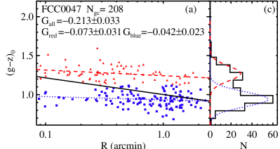
Figure 1.— Color profiles (left panels) and color distributions (right panels) of GC systems in two sample galaxies. a) GC system color profile of FCC 47 (NGC 1336), a GC system with a bimodal color distribution. Each small dot denotes a GC color coded for the blue and red subpopulation. The blue, red and black lines are the best linear fit of metal-poor, metal-rich and total GC populations. b) GC system color profile of unimodal galaxy FCC 153 (IC 335). c) GC color distribution of GCs in FCC 47. Blue and red curves represent the Gaussian fitting of blue and red GCs determined by KMM. d) GC color distribution for FCC 153, black curve represents the Gaussian fitting of all GCs.

The radial gradients are calculated by a linear least-squares fit between the GC color or metallicity and the logarithm of the radius, defined as:

$$G_{g-z} = \frac{\Delta(g-z)}{\Delta\log R}$$ (1)

$$G_{[Fe/H]} = \frac{\Delta[Fe/H]}{\Delta\log R}$$ (2)

In other words, we measure the change in color or metallicity per dex in radius. The color gradient errors are one-sigma errors and come from linear regression. To ensure adequate signal-to-noise, we restrict ourselves to the 78 galaxies with at least 20 GCs that meet our selection criteria ($p_{\rm GC}>0.95$). We subsequently eliminate VCC 1938 from our sample because of its close projected separation from the dwarf elliptical, VCC 1941. We also remove the S0/a transition galaxy, FCC167, due to uncertainties in measuring its stellar mass. This leaves us with a sample of 76 galaxies. If the galaxy has a bimodal GC color distribution, we calculate both the color gradient of whole GC system and the color gradient of each GC subpopulation. We divide the GCs in to red and blue using a simple color cut determined by the KMM probabilities. We tried various approaches, including running KMM as a function of radius, and allowing the dividing color to vary with radius using an iterative fitting process. In the former case, the number of GCs limited the effectiveness to only a handful of galaxies, and in the latter case our results did not change in a significant way so we ultimately chose to use the simplest method. Given the FOV of ACS ($3\farcm 4\times 3\farcm 4$), the maximum possible outer radius of our gradient measurements is $\sim 2\farcm 4$, which corresponds to 11.5 and 14.0 kpc at the distances of the Virgo and Fornax clusters, respectively.

The left panels of Figure 1 show color profiles of GC systems in FCC 47 (panel $a$) and FCC 153 (panel $b$). We can see from the figure that both red and blue GC systems in FCC 47 show negative color gradients with color becoming gradually bluer from the center to the outskirts of the galaxy. The gradients of the whole GC system is steeper than that of each subpopulation due to the dominance of blue GCs at large radii. The GC system in the unimodal galaxy FCC 153 also shows a shallower but significant negative color gradient.

For the two most luminous giant galaxies in the Virgo cluster: M49 (VCC 1226) and M87 (VCC 1316), the gradients are extended by including the GCs in nearby ACS fields. Because some targeted galaxies were located in the halos of the giants, and their own GC systems appear to be entirely stripped (see Peng et al. 2008 for details), we consider the GCs in these fields as part of the GC systems of the giant galaxies. For M49, we use VCC 1199 and 1192, extending our study to a radius of $4\farcm 5$ (22 kpc). For M87, we use VCC 1327, 1297, 1279, 1185 and 1250, which extends our study to a radius of $21\farcm 3$ (102 kpc). There are two similar cases in the Fornax cluster. FCC 202 is near FCC 213 ($4\farcm 6$, 27 kpc) and FCC 143 is near FCC 147 ($4\farcm 8$, 28 kpc).

3. Results

3.1. Color Gradients

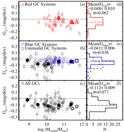
Figure 2.— Color gradients as a function of galaxy stellar mass (left panels) and gradient distributions (right panels). From top to bottom: red GC systems, blue and unimodal GC systems, and all GCs. The dotted lines in panel $a$, $b$, and $c$ denote the zero gradients. In panel $d$, $e$ and $f$, the dot-dashed lines describe the mean $G_{g-z}$ of red, blue and whole GC systems respectively. The dashed histogram in panel $e$ is the distribution of color gradients in unimodal galaxies. Big filled circles in panel $b$ and $c$ denote the mean gradients in given mass bins. The larger and thicker open symbols at the high mass ends of panels $a$ $b$ and $c$, denote the four galaxies whose profiles were extended by the use of neighboring ACS fields: M49, M87, FCC 213, and FCC 147 (see Section 2.3).

Figure 2 presents results for all 76 galaxies, showing the color gradient distribution (right panels), and the strength of the color gradients as a function of galaxy stellar mass (left panels). The stellar masses for the ACSVCS galaxies were taken from Peng et al. (2008), and the masses for the ACSFCS galaxies were calculated in the same way as described in that paper using $g$–$z$ photometry from the ACS images (Ferrarese et al., in prep) and $J$–$K$ colors from the Two Micron All Sky Survey (2MASS, Skrutskie et al. 2006). From top to bottom, this figure shows the color gradients of red GC populations, blue GC and unimodal populations, and whole GC systems, respectively. We combine the blue GCs and unimodal populations on the same plot because unimodal populations for low mass galaxies consist nearly entirely of blue GCs, and are likely the low mass extension of the blue GCs in more massive galaxies (see Peng et al. 2006a). Consistent with previous studies (e.g. Geisler et al. 1996; Rhode & Zepf 2001; Jordán et al. 2004a; Tamura et al. 2006; Harris 2009b), we find that the whole GC systems of most giant early-type galaxies have negative color gradients. We also find that not only giant galaxies, but also most intermediate- and low-mass galaxies show shallow but significant color gradients in their GC systems.

As described in Section 2.2 and 2.3, we calculate the color gradients of individual red and blue GC systems respectively if GCs display bimodal color distribution. Figure 2 shows that although the subpopulation gradients for individual galaxies are often not by themselves very significant, both red and blue GC systems have significant shallow negative color gradients when we combine data from many galaxies. The red and blue GC gradients have mean values equaling $-0.048\pm 0.010$ and $-0.041\pm 0.006$ respectively. The errors in the color gradients of individual GC systems are taken into account when calculating the mean color gradients and their errors. Color gradients of red GC populations are slightly steeper than that of blue GC systems and seem to show more scatter with dispersions $\sigma_{\rm{red}}=0.062$ and $\sigma_{\rm{blue}}=0.038$. Furthermore, both red and blue GC systems individually have much shallower color gradients than that of whole GC systems ($-0.112\pm 0.009$) with dispersion $\sigma_{\rm{all}}=0.077$.

Table 1 and 2 lists the color gradients of blue, red and whole GC systems for our sample galaxies. We only show the results for the 76 galaxies with more than 20 GCs that meet our selection.

In panels $b$ and $c$ of Figure 2, big filled circles display the mean color gradients in given mass bins with bin widths of 0.6 dex. For galaxies with $\mathcal{M}_{\star}\lesssim 10^{10}\mathcal{M}_{\odot}$, there appears to be a weak correlation between color gradients and galaxy mass, with color gradients tending to be shallower for dwarf galaxies. But for the higher mass galaxies, the trend is flattened, even reversed. In this figure, Virgo and Fornax galaxies are plotted together. We do not find a significant difference in behavior between galaxies in the different clusters.

3.2. Metallicity Gradients

Since most GCs are old, single stellar populations, trends in their integrated color are generally equated with trends in metallicity. Recent studies have found a non-linear but monotonic relation between metallicity and color of GCs (e.g., Harris & Harris 2002; Peng et al. 2006a; Blakeslee et al. 2010), with broadband color less sensitive at lower metallicity. Blakeslee et al. (2010) fit the color-metallicity relation from the data shown in (Peng et al. 2006a) using a quartic polynomial (their Equation 1). Although the conversion from color to metallicity is still uncertain and contains considerable scatter, we can use the Blakeslee et al. (2010) relation to derive a radial metallicity profile for each GC system. After conversion, the metallicity distribution of GC systems in many galaxies are not bimodal (see Yoon et al. 2006; Cantiello & Blakeslee 2007; Blakeslee et al. 2010), but interpreting this is beyond the scope of this paper (see also Spitler et al. 2008). In this work, we only use this relation to calculate the mean metallicity gradients of the entire GC system of each galaxy.

Figure 3.— The same as panel $c$ and $f$ of Figure 2, but with color gradients converted to metallicity for whole GC systems.

Figure 3 presents the distribution of metallicity gradients of all GCs and the gradient–mass relation. Similar to the color gradients, the GC systems of most galaxies have shallow but significant metallicity gradients with a mean value of $-0.387\pm 0.034$ with dispersion $\sigma_{[Fe/H]}=0.284$. The metallicity gradient–mass relation is also similar to the color gradient–mass relation shown in Figure 2.

Table 1Color and Metallicity gradients of GC systems of ACSVCS galaxies

Name	$N_{\textrm{GC}}$	$\log(\mathcal{M}_{\star}/\mathcal{M}_{\odot})$	$G_{\rm{\textrm{blue}}}$	$G_{\textrm{red}}$	$G_{\textrm{all}}$	$G_{\textrm{[Fe/H]}}$	$G_{\textrm{gal}}$
(1)	(2)	(3)	(4)	(5)	(6)	(7)	(8)
VCC 1226	$950$	$11.73$	$-0.032\pm 0.017$	$-0.037\pm 0.019$	$-0.139\pm 0.024$	$-0.493\pm 0.080$	$-0.058\pm 0.003$
VCC 1316	$2002$	$11.48$	$-0.049\pm 0.008$	$-0.049\pm 0.011$	$-0.171\pm 0.013$	$-0.570\pm 0.044$	$-0.015\pm 0.002$
VCC 1978	$709$	$11.53$	$-0.027\pm 0.027$	$-0.021\pm 0.023$	$-0.070\pm 0.036$	$-0.214\pm 0.117$	$-0.026\pm 0.002$
VCC 881	$256$	$11.46$	$-0.010\pm 0.036$	$-0.027\pm 0.044$	$-0.011\pm 0.049$	$-0.065\pm 0.180$	$9.999\pm 0.000$
VCC 798	$258$	$11.27$	$-0.075\pm 0.033$	$-0.099\pm 0.033$	$-0.150\pm 0.044$	$-0.543\pm 0.145$	$0.104\pm 0.006$
VCC 763	$408$	$11.37$	$-0.048\pm 0.025$	$-0.145\pm 0.034$	$-0.117\pm 0.040$	$-0.404\pm 0.137$	$-0.042\pm 0.003$
VCC 731	$772$	$11.35$	$-0.056\pm 0.024$	$-0.033\pm 0.021$	$-0.118\pm 0.030$	$-0.408\pm 0.091$	$-0.104\pm 0.002$
VCC 1535	$163$	$10.89$	$0.079\pm 0.040$	$-0.013\pm 0.045$	$-0.134\pm 0.068$	$-0.317\pm 0.227$	$0.133\pm 0.154$
VCC 1903	$244$	$10.92$	$-0.065\pm 0.032$	$-0.035\pm 0.030$	$-0.082\pm 0.044$	$-0.281\pm 0.132$	$-0.102\pm 0.004$
VCC 1632	$355$	$10.98$	$-0.045\pm 0.030$	$0.012\pm 0.031$	$-0.064\pm 0.044$	$-0.182\pm 0.128$	$-0.056\pm 0.004$
VCC 1231	$199$	$10.73$	$0.006\pm 0.030$	$0.017\pm 0.037$	$0.019\pm 0.047$	$0.035\pm 0.149$	$-0.056\pm 0.003$
VCC 2095	$75$	$10.72$	$\cdots$	$\cdots$	$-0.072\pm 0.067$	$-0.256\pm 0.272$	$-0.116\pm 0.002$
VCC 1154	$132$	$10.89$	$-0.125\pm 0.045$	$0.082\pm 0.057$	$-0.074\pm 0.067$	$-0.363\pm 0.218$	$-0.019\pm 0.002$
VCC 1062	$129$	$10.72$	$0.013\pm 0.045$	$0.032\pm 0.053$	$-0.130\pm 0.067$	$-0.473\pm 0.224$	$-0.086\pm 0.002$
VCC 2092	$52$	$10.68$	$-0.093\pm 0.067$	$0.095\pm 0.067$	$0.097\pm 0.103$	$0.163\pm 0.345$	$-0.132\pm 0.003$
VCC 369	$128$	$10.51$	$-0.002\pm 0.048$	$0.027\pm 0.055$	$0.073\pm 0.075$	$0.170\pm 0.230$	$-0.078\pm 0.003$
VCC 759	$112$	$10.65$	$-0.056\pm 0.035$	$0.023\pm 0.042$	$-0.048\pm 0.052$	$-0.221\pm 0.187$	$-0.060\pm 0.006$
VCC 1692	$93$	$10.53$	$0.011\pm 0.035$	$-0.073\pm 0.057$	$-0.094\pm 0.077$	$-0.205\pm 0.267$	$-0.077\pm 0.006$
VCC 1030	$118$	$10.12$	$-0.075\pm 0.037$	$-0.094\pm 0.048$	$-0.209\pm 0.064$	$-0.669\pm 0.217$	$-0.081\pm 0.009$
VCC 2000	$148$	$10.38$	$-0.057\pm 0.030$	$-0.072\pm 0.074$	$-0.188\pm 0.045$	$-0.684\pm 0.171$	$-0.092\pm 0.002$
VCC 685	$125$	$10.49$	$-0.035\pm 0.042$	$-0.087\pm 0.052$	$-0.210\pm 0.058$	$-0.734\pm 0.208$	$-0.026\pm 0.008$
VCC 1664	$104$	$10.42$	$\cdots$	$\cdots$	$-0.095\pm 0.062$	$-0.328\pm 0.175$	$-0.118\pm 0.003$
VCC 654	$23$	$10.36$	$\cdots$	$\cdots$	$-0.036\pm 0.121$	$-0.090\pm 0.600$	$-0.056\pm 0.005$
VCC 944	$62$	$10.46$	$-0.060\pm 0.055$	$-0.023\pm 0.061$	$-0.162\pm 0.088$	$-0.560\pm 0.319$	$-0.075\pm 0.002$
VCC 1720	$42$	$10.31$	$-0.154\pm 0.060$	$-0.149\pm 0.069$	$-0.178\pm 0.105$	$-0.733\pm 0.388$	$-0.118\pm 0.002$
VCC 355	$29$	$10.20$	$\cdots$	$\cdots$	$-0.345\pm 0.131$	$-1.455\pm 0.586$	$-0.083\pm 0.005$
VCC 1619	$44$	$10.24$	$\cdots$	$\cdots$	$-0.075\pm 0.091$	$-0.501\pm 0.367$	$-0.026\pm 0.001$
VCC 1883	$43$	$10.22$	$-0.079\pm 0.046$	$-0.021\pm 0.080$	$-0.144\pm 0.067$	$-0.452\pm 0.207$	$-0.018\pm 0.004$
VCC 1242	$78$	$10.18$	$-0.029\pm 0.036$	$-0.117\pm 0.040$	$-0.147\pm 0.057$	$-0.490\pm 0.177$	$-0.062\pm 0.002$
VCC 784	$43$	$10.23$	$\cdots$	$\cdots$	$-0.001\pm 0.114$	$-0.082\pm 0.406$	$-0.074\pm 0.003$
VCC 1537	$25$	$10.01$	$\cdots$	$\cdots$	$-0.342\pm 0.065$	$-1.068\pm 0.294$	$-0.058\pm 0.003$
VCC 778	$43$	$10.26$	$\cdots$	$\cdots$	$-0.137\pm 0.099$	$-0.387\pm 0.382$	$-0.064\pm 0.003$
VCC 1321	$22$	$9.84$	$\cdots$	$\cdots$	$-0.085\pm 0.078$	$-0.630\pm 0.426$	$-0.084\pm 0.004$
VCC 828	$48$	$10.14$	$0.032\pm 0.048$	$0.065\pm 0.107$	$-0.159\pm 0.077$	$-0.553\pm 0.365$	$-0.038\pm 0.002$
VCC 1630	$29$	$10.06$	$\cdots$	$\cdots$	$-0.199\pm 0.118$	$-1.005\pm 0.479$	$-0.060\pm 0.002$
VCC 1146	$53$	$9.94$	$\cdots$	$\cdots$	$-0.139\pm 0.062$	$-0.105\pm 0.105$	$-0.081\pm 0.003$
VCC 1025	$58$	$10.33$	$\cdots$	$\cdots$	$-0.210\pm 0.055$	$-0.801\pm 0.239$	$-0.113\pm 0.003$
VCC 1303	$37$	$10.02$	$\cdots$	$\cdots$	$-0.038\pm 0.042$	$-0.271\pm 0.262$	$-0.113\pm 0.003$
VCC 1913	$36$	$10.03$	$\cdots$	$\cdots$	$-0.037\pm 0.070$	$-0.235\pm 0.275$	$-0.079\pm 0.004$
VCC 1125	$39$	$9.91$	$\cdots$	$\cdots$	$-0.080\pm 0.064$	$-0.382\pm 0.302$	$0.042\pm 0.004$
VCC 1475	$52$	$9.89$	$\cdots$	$\cdots$	$-0.013\pm 0.059$	$0.067\pm 0.266$	$-0.044\pm 0.004$
VCC 1178	$58$	$9.85$	$\cdots$	$\cdots$	$-0.102\pm 0.063$	$-0.450\pm 0.228$	$-0.005\pm 0.004$
VCC 1283	$36$	$9.96$	$\cdots$	$\cdots$	$-0.113\pm 0.099$	$-0.533\pm 0.324$	$-0.047\pm 0.003$
VCC 1261	$22$	$9.69$	$\cdots$	$\cdots$	$-0.033\pm 0.070$	$-0.202\pm 0.235$	$-0.007\pm 0.004$
VCC 698	$83$	$9.98$	$\cdots$	$\cdots$	$-0.068\pm 0.051$	$-0.294\pm 0.235$	$0.018\pm 0.006$
VCC 1910	$34$	$9.32$	$\cdots$	$\cdots$	$-0.158\pm 0.074$	$-0.703\pm 0.315$	$-0.017\pm 0.005$
VCC 856	$24$	$9.35$	$\cdots$	$\cdots$	$-0.038\pm 0.065$	$-0.173\pm 0.274$	$0.001\pm 0.006$
VCC 1087	$43$	$9.52$	$\cdots$	$\cdots$	$-0.110\pm 0.045$	$-0.383\pm 0.228$	$-0.057\pm 0.010$
VCC 1861	$28$	$9.46$	$\cdots$	$\cdots$	$-0.253\pm 0.107$	$-0.974\pm 0.479$	$-0.009\pm 0.007$
VCC 1431	$40$	$9.34$	$\cdots$	$\cdots$	$-0.078\pm 0.054$	$-0.316\pm 0.196$	$0.065\pm 0.012$
VCC 1528	$28$	$9.21$	$\cdots$	$\cdots$	$-0.124\pm 0.055$	$-0.616\pm 0.333$	$-0.046\pm 0.006$
VCC 2019	$20$	$9.01$	$\cdots$	$\cdots$	$-0.021\pm 0.062$	$-0.364\pm 0.380$	$-0.084\pm 0.008$
VCC 1545	$27$	$9.15$	$\cdots$	$\cdots$	$-0.122\pm 0.053$	$-0.341\pm 0.266$	$-0.143\pm 0.005$
VCC 1407	$22$	$9.09$	$\cdots$	$\cdots$	$0.040\pm 0.050$	$0.178\pm 0.207$	$0.011\pm 0.004$
VCC 1539	$24$	$8.72$	$\cdots$	$\cdots$	$-0.079\pm 0.073$	$-0.363\pm 0.359$	$0.113\pm 0.019$

Table 2Color and Metallicity gradients of GC systems of ACSFCS galaxies

Name	$N_{\textrm{GC}}$	$\log(\mathcal{M}_{\star}/\mathcal{M}_{\odot})$	$G_{\rm{\textrm{blue}}}$	$G_{\textrm{red}}$	$G_{\textrm{all}}$	$G_{\textrm{[Fe/H]}}$	$G_{\textrm{gal}}$
(1)	(2)	(3)	(4)	(5)	(6)	(7)	(8)
FCC 21	$231$	$11.88$	$-0.109\pm 0.040$	$-0.224\pm 0.041$	$-0.241\pm 0.049$	$-0.796\pm 0.154$	$-0.074\pm 0.010$
FCC 213	$1067$	$11.42$	$-0.046\pm 0.019$	$-0.041\pm 0.019$	$-0.086\pm 0.023$	$-0.304\pm 0.070$	$-0.015\pm 0.002$
FCC 219	$297$	$11.14$	$-0.047\pm 0.038$	$-0.119\pm 0.027$	$-0.182\pm 0.048$	$-0.681\pm 0.154$	$-0.019\pm 0.002$
NGC 1340	$151$	$10.99$	$0.008\pm 0.037$	$-0.044\pm 0.066$	$-0.024\pm 0.048$	$-0.080\pm 0.219$	$-0.073\pm 0.005$
FCC 276	$280$	$10.67$	$-0.050\pm 0.027$	$-0.029\pm 0.032$	$-0.176\pm 0.037$	$-0.602\pm 0.118$	$-0.067\pm 0.003$
FCC 147	$264$	$10.69$	$-0.047\pm 0.022$	$0.025\pm 0.039$	$-0.154\pm 0.029$	$-0.516\pm 0.090$	$-0.042\pm 0.003$
IC 2006	$97$	$10.38$	$-0.027\pm 0.048$	$-0.173\pm 0.060$	$-0.171\pm 0.074$	$-0.515\pm 0.232$	$-0.123\pm 0.004$
FCC 83	$217$	$10.51$	$-0.002\pm 0.021$	$-0.108\pm 0.031$	$-0.089\pm 0.037$	$-0.248\pm 0.115$	$-0.105\pm 0.002$
FCC 184	$230$	$10.82$	$-0.037\pm 0.046$	$-0.089\pm 0.048$	$-0.013\pm 0.079$	$-0.074\pm 0.248$	$-0.011\pm 0.001$
FCC 63	$163$	$10.43$	$-0.045\pm 0.035$	$-0.082\pm 0.040$	$-0.171\pm 0.046$	$-0.513\pm 0.167$	$-0.120\pm 0.006$
FCC 193	$25$	$10.48$	$\cdots$	$\cdots$	$0.023\pm 0.140$	$0.056\pm 0.475$	$-0.107\pm 0.003$
FCC 170	$44$	$10.29$	$\cdots$	$\cdots$	$-0.137\pm 0.074$	$-0.578\pm 0.350$	$-0.007\pm 0.005$
FCC 153	$33$	$9.94$	$\cdots$	$\cdots$	$-0.112\pm 0.059$	$-0.502\pm 0.340$	$0.078\pm 0.012$
FCC 177	$45$	$9.82$	$\cdots$	$\cdots$	$-0.097\pm 0.050$	$-0.401\pm 0.291$	$0.200\pm 0.014$
FCC 47	$206$	$9.97$	$-0.043\pm 0.021$	$-0.074\pm 0.031$	$-0.208\pm 0.033$	$-0.687\pm 0.116$	$-0.093\pm 0.004$
FCC 190	$106$	$9.87$	$-0.087\pm 0.022$	$0.023\pm 0.064$	$-0.116\pm 0.030$	$-0.619\pm 0.156$	$-0.005\pm 0.004$
FCC 249	$115$	$9.99$	$\cdots$	$\cdots$	$-0.115\pm 0.041$	$-0.446\pm 0.165$	$-0.083\pm 0.007$
FCC 148	$58$	$10.03$	$0.006\pm 0.043$	$0.019\pm 0.049$	$0.042\pm 0.076$	$0.161\pm 0.305$	$0.189\pm 0.010$
FCC 255	$53$	$9.56$	$-0.035\pm 0.034$	$-0.044\pm 0.041$	$-0.147\pm 0.044$	$-0.526\pm 0.179$	$0.012\pm 0.005$
FCC 277	$22$	$9.88$	$\cdots$	$\cdots$	$-0.300\pm 0.119$	$-0.995\pm 0.501$	$-0.055\pm 0.003$
FCC 182	$30$	$9.40$	$\cdots$	$\cdots$	$0.080\pm 0.078$	$0.204\pm 0.278$	$-0.036\pm 0.010$

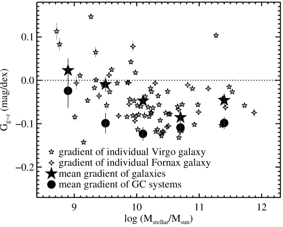
Figure 4.— Color gradients of galaxies and GC systems binned by mass as a function of stellar mass, $\mathcal{M}_{\star}$. Small open stars with error bars are the gradients and errors in individual galaxies. Filled stars and circles describe the mean color gradients and errors of galaxies and GC systems in given mass bins.

3.3. The Gradient–Mass Relation and Comparison to Field Stars

We have seen that the strength of the GC systems color gradient varies as a function of galaxy mass. Similar behavior has been seen in the color gradients of the field stars for galaxies in other studies. One advantage of the ACSVCS and ACSFCS data is that we can also measure color gradients for the host galaxies using the exact same filters that we use for the GCs, allowing us to make a direct comparison between the two galactic components.

Ferrarese et al. (2006) measured the isophotal light profiles of 100 early-type galaxies in the ACSVCS in both the $g$ and $z$ band. The light profiles of 43 ACSFCS galaxies are measured by using the same method (Ferrarese et al., in prep). The calculations of the color gradients of these galaxies are based on their surface photometry. To remove the effect of nuclei of early-type galaxies (about $2\%$ of effective radius, see Côté et al. 2006, 2007) and eliminate the significant contamination of sky background in outskirts, we measure the color gradients in the range from $0.02~{}R_{e}$ to $R_{e}$. The definition of color gradient is the same as that for GC systems (Equation 1). We list the stellar color gradients for the ACSVCS/FCS galaxies in Table 1.

Figure 4 shows the relationship between the field star color gradients and galaxy stellar mass, $\mathcal{M}_{\star}$. Larger stars denote the mean gradient in a given mass bin. Similar to what has been found in other studies, the color gradients of the ACSVCS/FCS early-type galaxies are mostly negative, with low mass galaxies having flat or positive gradients. We find no significant difference between color gradients of galaxies in the Virgo and Fornax. In the mean, the steepest gradients are found in intermediate-mass galaxies, which is consistent with the finding of Tortora et al. (2010a) from SDSS surface photometry of galaxies. The circles in Figure 4 show the mean values for color gradients of GC systems, shown in bottom panel of Figure 2. We can see that the color gradients of GC systems are systematically steeper than those of the field stars, but that the gradient–mass relation is similar in shape to that of stellar systems of galaxies.

At the bright end, the color gradients of GC systems seems to be getting shallower again, but there is an important caveat. The ACS observations of our sample galaxies have field view of $3\farcm 4\times 3\farcm 4$, which at the distance of the Virgo Cluster is roughly 16 kpc on a side. For the massive galaxies, we are only probing the innermost regions of the halo, even when using fields that observed neighboring galaxies. Rhode & Zepf (2001), in a wide-field study of the GC system in M49 (NGC 4472, VCC 1226), found color gradients within $8\arcmin$, but also found that the gradient disappeared when expanding the radius to $22\arcmin$. Harris (2009a) measured color gradients for the GCs in M87 and found detectable gradients out to $\sim 60$ kpc, or $12\farcm 5$, a roughly similar radial scale. In this work, we have mostly only calculated color gradients of the central part of the GC systems of massive galaxies due to the limited field of view of ACS, so for massive galaxies these color gradients are best described as those for “inner halo” GCs. A more comprehensive study of GC system color gradients will require wide-field imaging, such as that being taken for the Next Generation Virgo Cluster Survey (Ferrarese et al. 2011, in prep.).

4. Discussion

4.1. A Note on Projection Effects

When we calculate the GC system color gradients, we use projected galactocentric distances, not the true three-dimensional distances to the galaxy centers. Projecting the GC system onto the plane of the sky weakens the measured gradients, as GCs projected onto the center are actually a mix of GCs at all radii. This is less of a problem for more centrally concentrated systems (i.e., more steeply rising density profiles toward the center). Because the distribution of red GCs can be more concentrated than blue GCs, the projection effects for the two subpopulations could be different.

In order to test the affects of projecting real gradients into the plane of the sky, we provide one test case. Côté et al. (2001) deprojected the spatial distribution of the red and blue GC subpopulations in the galaxy M87. The projections of the model density distribution are consistent with the observed surface density of GCs. They obtained:

$$n_{red}(r) = (\frac{r}{3.3~{}{\rm kpc}})^{-1}(1+\frac{r}{3.3~{}{\rm kpc}})^{-2},~{}r<95~{}{\rm kpc}$$ (3)

$$n_{blue}(r) = (\frac{r}{20.5{\rm kpc}})^{-1}(1+\frac{r}{20.5{\rm kpc}})^{-2},r<125~{}{\rm kpc}$$ (4)

We assume that the initial color gradient of GC systems are $-0.15$ and project the model density distribution into two dimensions. The resulting projected color profiles are shown in Figure 5. The projection effect flattens the gradient of both red and blue GC systems to $-0.134$ and $-0.132$, respectively. Because the blue GCs are more extended than the red ones, the flattening is slightly more obvious in the gradient of blue GC system. The total effect of projection in this case, however, is relatively small, roughly 12%, and the relative effect between the red and blue GCs is negligible. We do not correct for projection effects because we do not know the three-dimensional density profiles of the GC systems. We simply note that the true radial color gradients for these GC systems are slightly steeper than the projected gradients, but that for a realistic density profile of GCs, this correction is likely to be of the order of $\sim 10\%$.

Figure 5.— A simulated GC system color profile. Solid line is the intrinsic profile, dashed and dotted lines denote color profiles of red and blue GC populations when projected onto the plane of the sky.

4.2. Gradient-Induced Bias in the Colors of GC Subpopulations

Our results show that the GC systems of early-type galaxies display significant negative color gradients, which is consistent with previous work (e.g., Strom et al., 1981; Geisler et al., 1996; Rhode & Zepf, 2004; Jordán et al., 2004a; Cantiello et al., 2007). However, there exists more uncertainty about whether individual GC subpopulations display color gradients or not. Some previous studies have found shallow gradients in individual GC subpopulations (e.g., Bassino et al., 2006; Harris, 2009a, b) while other studies have not (e.g., Forbes et al., 2004; Cantiello et al., 2007; Kundu & Zepf, 2007). In this work, we find that only a few of the individual GC subpopulations show significant gradients ($>3\sigma$), but the overall trend is obvious when measured over 39 galaxies, i.e., individual GC subpopulations display negative gradients statistically. It is the first homogeneous study of color gradients of GC systems in early-type galaxies, and emphasizes the power of using a large, homogeneous sample of galaxies.

One consequence of this result could be on the mean measured colors of the subpopulations. The studies with the highest precision photometry and least contamination have often used HST imaging (e.g., Larsen et al., 2001; Peng et al., 2006a) which necessarily has a small field of view relative to the largest nearby GC systems. Results from these studies have shown that the mean color of the blue and red GC subpopulations is a function of galaxy mass or luminosity, where more massive galaxies have redder GCs, in the mean. This has generally been interpreted as a mass–metallicity relation for GC systems (as opposed to for individual GCs). The correlation for metal-poor GCs, although weaker than that for the red GCs, has drawn particular interest because it implies a connection between the earliest forming GCs and the final halos in which they reside (Larsen et al., 2001; Burgarella et al., 2001; Strader et al., 2004; Peng et al., 2006a).

Given the fixed and relatively small field of view for the instruments, there is a significant aperture sampling effect that varies across the studied range of galaxy mass. Peng et al. (2008) showed that for galaxies with $M_{B}>-18$, the entire GC system typically fits within the ACS field of view. At higher luminosities, the ACS field will miss some fraction of the outer regions. This fraction can be as high as $\sim 90\%$, in the case of M87. This bias toward the centers of galaxies would not matter if the GC subpopulations did not possess color gradients. We have found, however, that they typically have gradients of 0.04–0.05 mag/dex in ($g$–$z$). This results in a bias where the most massive galaxies are sampled where the GCs are most red. This would particularly affect the blue GCs, which can have a more extended spatial distribution.

Although the resolution of this issue will ultimately require precision wide-field imaging, we can estimate the degree of bias that color gradients may have introduced. For the most massive galaxies in Virgo, such as M49, M87, and M60, the effective radii ($R_{e,\rm GCs}$) of the GC populations are 42, 41, and 24 kpc, respectively. This was determined using Sérsic fits to the GC spatial distribution from ACSVCS data and published photometry (McLaughlin, 1999; Rhode & Zepf, 2001). The mean projected radius for the GCs observed in the ACS field, and for which the subpopulations colors were measured in Peng et al. (2006a), is roughly 5 kpc. Given the gradients for the red and blue populations measured in this paper (Table 1), we can infer the expected difference between the mean color in the ACS field and the mean color at $1R_{e,\rm GCs}$, which should roughly represent the mean color of the entire GC subpopulation if the color gradient is constant at all radii. The color difference, $\Delta_{g-z}(ACS-R_{e,\rm GCs})$, for M49, M87, and M60 is: $0.031$ mag, $0.046$ mag, and $0.019$ mag, respectively.

Could such a shift to the blue affect the previously published correlations between galaxy mass and GC subpopulation metallicity? We estimate $\Delta_{g-z}$ as a function of galaxy $M_{B}$ in the ACSVCS sample for easy comparison with the analysis in Peng et al. (2006a). We use the measured mean colors within the HST/ACS field of view from Table 4 of Peng et al. (2006a), $R_{e,\rm GCs}$ for the GC systems in the ACSVCS galaxies (Peng et al. 2008; Peng et al., in prep), and the mean color gradients for the red and blue GC subpopulations ($-0.048$ and $-0.041$, respectively, Figure 2) to infer the mean color for the red and blue subpopulations at $R_{e,GCs}$, which we take to be representative of the entire population. We weight each galaxy’s contribution to $\Delta_{g-z}$ by their total number of GCs from Peng et al. (2008).

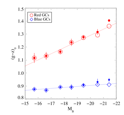
Figure 6.— Mean colors of red (circles) and blue GCs (diamonds) as a function of galaxy luminosity ($M_{B}$) with data from Peng et al. (2006) (filled points) and inferred corrections to a common radius of $R_{e,\rm GCs}$ (open points). The correction is only important for the most luminous galaxies. The dotted lines show linear fits to the data with inferred correction. The slope of the blue GCs is -0.007, only half the value when fitting the original data.

Figure 6 mirrors Figure 8a of Peng et al. (2006a) and plots the mean colors versus galaxy $M_{B}$, both measured with ACS (solid points) and inferred at $R_{e,\rm GCs}$ (open points). As expected, the correction is only important for the two most luminous bins in $M_{B}$. Whereas the relation for the red GCs is not significantly affected, as it was originally quite steep, the slope for the blue GC relation is noticeably smaller. The fit to the original measurements gave a blue GC slope of $-0.0126\pm 0.0025$, a nonzero slope at the $5\sigma$ level. The fit to the newly inferred mean colors produces a slope of $-0.0069\pm 0.0025$ (systematic errors from the correction process are not included). This shallower slope is now only significant at $2.8\sigma$, and could potentially be even less significant if more accurate color gradients on the outer regions are measured to be steeper than what we have measured.

We want to emphasize that this exercise is far from conclusive, and only serves to warn that color gradients in the GC subpopulations will potentially affect conclusions drawn from imaging the central regions of galaxies. Similar biases have been noted for the color-magnitude relation of early-type galaxies where colors are measured in fixed apertures (Scodeggio, 2001). The correction that we infer out to $R_{e,\rm GCs}$ assumes a constant color gradient over the entire GC system. This assumption is unverified, and probably provides an upper limit on the possible correction, given the results of Rhode & Zepf (2001) and Harris (2009b) who find a flattening gradient at large radius. Nevertheless, a shallower (or potentially non-existent) relation between the mean color (metallicity) of metal-poor GCs and their host galaxy mass will have implications for understanding the formation of GC systems, and the solution to this problem awaits high-quality wide-field data (e.g., Rhode & Zepf 2004).

4.3. The Formation of GC systems and Their Hosts

That GC systems should have negative color (metallicity) gradients is perhaps not surprising given that GC formation is by its very nature a product of high star formation efficiency. Most models predict that high efficiency of star formation plus metal retention leads to more enriched populations at the centers of galaxies. Interestingly, even though GCs are among the oldest objects in galaxies, and thus have presumably experienced the largest amount of merger-induced radial mixing of any stellar population, the color gradients in most intermediate- and high-mass galaxies are still significantly negative.

Di Matteo et al. (2009) investigated the survival of metallicity gradient after a major dry merger. For ellipticals with similar initial gradients, they concluded that the final gradient is about 0.6 times of the initial after a major dry merger. Dissipational mergers, however, can either flatten or enhance gradients, depending on the initial gradients and the amount of gas involved. This dependence on merger history is one of the reasons why gradients in massive galaxies are expected to have larger dispersion. We have very few galaxies on the high-mass end, so it is difficult for us to probe the dispersion in GC system color gradients in this mass range. For the high-mass galaxies in our sample, we are also only probing the very inner halo, so it is possible that the gradients in this region are either more robust to dilution or had the strongest initial gradients. The color gradients for blue GCs (presumably the oldest GCs) in massive galaxies are detectable but shallower than at lower masses, and this may be a sign that mergers have played a part in their history. It would be interesting to extend this study to wider fields of view for the more massive galaxies.

We find that the mean gradients for the red and blue subpopulations are similar in magnitude ($-0.048$ and $-0.041$, respectively), but its interpretation is confounded by the uncertain conversion from ($g-z$) to metallicity. Both the Peng et al. (2006a) and Blakeslee et al. (2010) transformations have slopes that are roughly 3–4 times steeper at the mean blue GC color than at the mean red GC color. By extension, the true metallicity gradient for metal-poor GCs should be 3–4 times steeper than that for metal-rich GCs (given their similar gradients in color). This would be a fairly remarkable difference between the two populations, but is still entirely dependent on the assumed color-metallicity relation. We plan to revisit this question when the transformation from ($g$–$z$) is better understood.

The relationship between the color gradients of GC systems and host galaxy mass offers some interesting insights into the formation and evolution of stellar halos in early-type galaxies. Even for measurements of color gradients from galaxy surface photometry, it was only relatively recently that the data quality and mass range probed has been sufficient to study trends in galaxy mass (e.g., Forbes et al. 2005; Spolaor et al. 2009; Rawle et al. 2010; Tortora et al. 2010a). Tortora et al. (2010b) have also run simulations to show that environment can also play a role in the observed gradients. Our results show that the shape of gradient–mass relation for GC systems is similar to that for the galaxies themselves, with a minimum around $\approx 10^{10}\mathcal{M}_{\odot}$ (Figure 2). That the GC color gradients are universally steeper than those for the field stars is an interesting result. If the GCs formed in higher efficiency star forming events than the bulk of the field stars (e.g., Peng et al. 2008), then that might result in steeper gradients. One caveat for the interpretation, however, is that the total GC gradients are actually a combination of the red and blue GC populations, which may not have formed contemporaneously in the present-day halo. The steeper gradients are likely a combination of the increasing fraction of blue GCs and the increasing specific frequency of GCs at lower metallicity (Harris & Harris, 2002). The color gradients for the individual GC populations are similar in magnitude, if not slightly shallower than the gradients for the field stars.

The shape of the gradient–mass relation for both GC systems and field stars is broadly consistent with a model where color (metallicity) gradients are increasingly steeper in higher mass halos due to metal retention, but then are diluted in the highest-mass galaxies ($\mathcal{M}_{\star}\gtrsim 10^{10}\mathcal{M}_{\odot}$) due to the increasing importance of mergers in their evolution. One difference between the GCs and the stars is that the stars in some dwarfs exhibit significantly positive color gradients, which are often interpreted as due to age gradients (age increasing with radius) (e.g., La Barbera & de Carvalho, 2009; Spolaor et al., 2010). This is not difficult to produce if there has been recent low level star formation at the galaxy center. However, we do not see any case of this for the GC systems, nor might we expect to as the star formation rate density required to produce young GCs is much higher than needed to produce a slight age gradient in the field. We notice that there is a prominent outlier in Figure 4, VCC 798 (M85) with mass $\sim 10^{11.27}\mathcal{M}_{\odot}$, which has a steep positive color gradient. This galaxy is known as a young, gas-rich merger remnant (e.g., Schweizer & Seitzer, 1992; Peng et al., 2006b) and hosts a large-scale stellar disk (Ferrarese et al., 2006). During the gas-rich merger, the central starburst produced a young, blue stellar population in the center of galaxy. Therefore, the positive color gradients are common in gas-rich merger remnant (e.g., Yamauchi & Goto, 2005). However, the color gradient of the GC system in VCC 798 is negative and quite normal. One of the possible reasons is that the number of GCs formed during the merger is negligible compared to the preexisting old GC population. The fact that the GC systems of dwarf galaxies have shallow or flat color gradients suggests that metal retention and mixing were not efficient during the epoch of GC formation.

5. Conclusion

We use HST imaging from the ACS Virgo and Fornax Cluster Surveys to conduct the first large-scale study of globular cluster system radial color gradients. We present results for 76 early-type galaxies, measuring ($g$–$z$) color gradients for GC systems across a range in galaxy stellar mass ($8.7<\log(\mathcal{M}_{\star}/\mathcal{M}_{\odot})<11.8$). For 39 galaxies whose GC systems show significantly bimodal color distributions, we also measure the color gradients in the GC subpopulations. Using the surface photometry of ACSVCS galaxies from Ferrarese et al. (2006), we measure the radial color gradients of the field stars in the same galaxies and same filters, allowing a direct comparison of GC and field star radial gradients. We caution that the FOV of ACS means we only measure the central part of many large galaxies, which may introduce an aperture bias if the color gradient of galaxies are not constant with the radius. We find that:

1. GC systems as a whole have negative color gradients, with an average gradient over the entire sample of $-0.112\pm 0.009$ mag in ($g-z$) per dex in radius.

2. On average, red and blue GC subpopulations also show significantly negative color gradients at the mean level of $-0.048\pm 0.010$ and $-0.041\pm 0.006$, respectively. Although a gradient is sometimes difficult to detect for any individual galaxy, the combined sample shows this property with higher signal-to-noise.

3. We find a relationship between GC system gradient strength and galaxy stellar mass, where the gradients are flat at low mass, increasingly negative with mass until $\mathcal{M}_{\star}\approx 10^{10}\mathcal{M}_{\odot}$ and then staying constant or less negative at higher mass. This trend parallels the gradient–mass relationship we find for the field stars in the ACSVCS galaxies. The GC system gradients are systematically steeper than that for the field stars, which is likely a reflection of the dominance of blue GCs at large radius. These observed trends, however, are limited by the small number of galaxies at high and low mass in our sample.

4. Color gradients in the GC subpopulations can cause a bias in the measurement of the mean colors of GCs when the data only covers the central region of the galaxy. We infer a correction using the measured gradients and find that the slope between the mean color of metal-poor GCs and the luminosity of their hosts can be reduced by nearly a factor of two from previous measurements, raising questions about its level of significance.

5. The shape of the gradient–mass relation for GC systems is consistent with picture where the formation and chemical enrichment of the GC system becomes more efficient as the mass of the host galaxy increases, but is further affected by significant merging and radial mixing in the most massive galaxies.

6. In a test case, the intrinsic, three-dimensional color gradients are likely to be roughly $\sim 10\%$ steeper than the projected gradients given a reasonable spatial distribution of GCs.

References

- Ashman et al. (1994) Ashman, K. M., Bird, C. M., & Zepf, S. E. 1994, AJ, 108, 2348
- Bassino et al. (2006) Bassino, L. P., Faifer, F. R., Forte, J. C., Dirsch, B., Richtler, T., Geisler, D., & Schuberth, Y. 2006, A&A, 451, 789
- Bekki & Shioya (1999) Bekki, K., & Shioya, Y. 1999, ApJ, 513, 108
- Blakeslee et al. (2010) Blakeslee, J. P., Cantiello, M., & Peng, E. W. 2010, ApJ, 710, 51
- Blakeslee et al. (2009) Blakeslee, J. P., et al. 2009, ApJ, 694, 556
- Burgarella et al. (2001) Burgarella, D., Kissler-Patig, M., & Buat, V. 2001, AJ, 121, 2647
- Cantiello & Blakeslee (2007) Cantiello, M., & Blakeslee, J. P. 2007, ApJ, 669, 982
- Cantiello et al. (2007) Cantiello, M., Blakeslee, J. P., & Raimondo, G. 2007, ApJ, 668, 209
- Chiosi & Carraro (2002) Chiosi, C., & Carraro, G. 2002, MNRAS, 335, 335
- Côté et al. (2001) Côté, P., et al. 2001, ApJ, 559, 828
- Côté et al. (2004) —. 2004, ApJS, 153, 223
- Côté et al. (2006) —. 2006, ApJS, 165, 57
- Côté et al. (2007) —. 2007, ApJ, 671, 1456
- Di Matteo et al. (2009) Di Matteo, P., Pipino, A., Lehnert, M. D., Combes, F., & Semelin, B. 2009, A&A, 499, 427
- Ferrarese et al. (2006) Ferrarese, L., et al. 2006, ApJS, 164, 334
- Forbes et al. (2005) Forbes, D. A., Sánchez-Blázquez, P., & Proctor, R. 2005, MNRAS, 361, L6
- Forbes et al. (2004) Forbes, D. A., et al. 2004, MNRAS, 355, 608
- Forte et al. (2001) Forte, J. C., Geisler, D., Ostrov, P. G., Piatti, A. E., & Gieren, W. 2001, AJ, 121, 1992
- Franx et al. (1989) Franx, M., Illingworth, G., & Heckman, T. 1989, AJ, 98, 538
- Gebhardt & Kissler-Patig (1999) Gebhardt, K., & Kissler-Patig, M. 1999, AJ, 118, 1526
- Geisler et al. (1996) Geisler, D., Lee, M. G., & Kim, E. 1996, AJ, 111, 1529
- Hansen et al. (2007) Hansen, B. M. S., et al. 2007, ApJ, 671, 380
- Harris (2009a) Harris, W. E. 2009a, ApJ, 703, 939
- Harris (2009b) —. 2009b, ApJ, 699, 254
- Harris & Harris (2002) Harris, W. E., & Harris, G. L. H. 2002, AJ, 123, 3108
- Jordán et al. (2004a) Jordán, A., Côté, P., West, M. J., Marzke, R. O., Minniti, D., & Rejkuba, M. 2004a, AJ, 127, 24
- Jordán et al. (2004b) Jordán, A., et al. 2004b, ApJS, 154, 509
- Jordán et al. (2005) —. 2005, ApJ, 634, 1002
- Jordán et al. (2006) —. 2006, ApJ, 651, L25
- Jordán et al. (2007a) —. 2007a, ApJS, 169, 213
- Jordán et al. (2007b) —. 2007b, ApJS, 171, 101
- Jordán et al. (2009) —. 2009, ApJS, 180, 54
- Kawata & Gibson (2003) Kawata, D., & Gibson, B. K. 2003, MNRAS, 340, 908
- Kobayashi (2004) Kobayashi, C. 2004, MNRAS, 347, 740
- Kobayashi & Arimoto (1999) Kobayashi, C., & Arimoto, N. 1999, ApJ, 527, 573
- Kundu & Whitmore (2001) Kundu, A., & Whitmore, B. C. 2001, AJ, 121, 2950
- Kundu & Zepf (2007) Kundu, A., & Zepf, S. E. 2007, ApJ, 660, L109
- Kuntschner et al. (2006) Kuntschner, H., et al. 2006, MNRAS, 369, 497
- La Barbera & de Carvalho (2009) La Barbera, F., & de Carvalho, R. R. 2009, ApJ, 699, L76
- Larsen et al. (2001) Larsen, S. S., Brodie, J. P., Huchra, J. P., Forbes, D. A., & Grillmair, C. J. 2001, AJ, 121, 2974
- Lee et al. (1998) Lee, M. G., Kim, E., & Geisler, D. 1998, AJ, 115, 947
- Liu et al. (2009) Liu, C., Shen, S., Shao, Z., Chang, R., Hou, J., Yin, J., & Yang, D. 2009, RAA, 9, 1119
- MacArthur et al. (2004) MacArthur, L. A., Courteau, S., Bell, E., & Holtzman, J. A. 2004, ApJS, 152, 175
- Marín-Franch et al. (2009) Marín-Franch, A., et al. 2009, ApJ, 694, 1498
- Masters et al. (2010) Masters, K. L., et al. 2010, ApJ, 715, 1419
- McLachlan & Basford (1988) McLachlan, G. J., & Basford, K. E. 1988, Mixture models. Inference and applications to clustering (New York: M. Dekker)
- McLaughlin (1999) McLaughlin, D. E. 1999, AJ, 117, 2398
- Mei et al. (2007) Mei, S., et al. 2007, ApJ, 655, 144
- Michard (2005) Michard, R. 2005, A&A, 441, 451
- Mieske et al. (2006) Mieske, S., et al. 2006, ApJ, 653, 193
- Mieske et al. (2010) —. 2010, ApJ, 710, 1672
- Peletier et al. (1990) Peletier, R. F., Davies, R. L., Illingworth, G. D., Davis, L. E., & Cawson, M. 1990, AJ, 100, 1091
- Peng et al. (2006a) Peng, E. W., et al. 2006a, ApJ, 639, 95
- Peng et al. (2006b) —. 2006b, ApJ, 639, 838
- Peng et al. (2008) —. 2008, ApJ, 681, 197
- Pipino et al. (2010) Pipino, A., D’Ercole, A., Chiappini, C., & Matteucci, F. 2010, MNRAS, 407, 1347
- Puzia et al. (2006) Puzia, T. H., Kissler-Patig, M., & Goudfrooij, P. 2006, ApJ, 648, 383
- Rawle et al. (2010) Rawle, T. D., Smith, R. J., & Lucey, J. R. 2010, MNRAS, 401, 852
- Rawle et al. (2008) Rawle, T. D., Smith, R. J., Lucey, J. R., & Swinbank, A. M. 2008, MNRAS, 389, 1891
- Rhode & Zepf (2001) Rhode, K. L., & Zepf, S. E. 2001, AJ, 121, 210
- Rhode & Zepf (2004) —. 2004, AJ, 127, 302
- Roche et al. (2010) Roche, N., Bernardi, M., & Hyde, J. 2010, MNRAS, 407, 1231
- Schweizer & Seitzer (1992) Schweizer, F., & Seitzer, P. 1992, AJ, 104, 1039
- Scodeggio (2001) Scodeggio, M. 2001, AJ, 121, 2413
- Searle & Zinn (1978) Searle, L., & Zinn, R. 1978, ApJ, 225, 357
- Skrutskie et al. (2006) Skrutskie, M. F., et al. 2006, AJ, 131, 1163
- Spitler et al. (2008) Spitler, L. R., Forbes, D. A., & Beasley, M. A. 2008, MNRAS, 389, 1150
- Spolaor et al. (2010) Spolaor, M., Kobayashi, C., Forbes, D. A., Couch, W. J., & Hau, G. K. T. 2010, MNRAS, 408, 272
- Spolaor et al. (2009) Spolaor, M., Proctor, R. N., Forbes, D. A., & Couch, W. J. 2009, ApJ, 691, L138
- Strader et al. (2004) Strader, J., Brodie, J. P., & Forbes, D. A. 2004, AJ, 127, 3431
- Strom et al. (1981) Strom, S. E., Strom, K. M., Wells, D. C., Forte, J. C., Smith, M. G., & Harris, W. E. 1981, ApJ, 245, 416
- Tamura et al. (2006) Tamura, N., Sharples, R. M., Arimoto, N., Onodera, M., Ohta, K., & Yamada, Y. 2006, MNRAS, 373, 601
- Tortora et al. (2010a) Tortora, C., Napolitano, N. R., Cardone, V. F., Capaccioli, M., Jetzer, P., & Molinaro, R. 2010a, MNRAS, 407, 144
- Tortora et al. (2010b) Tortora, C., Romeo, A. D., Napolitano, N. R., Antonuccio-Delogu, V., Meza, A., Sommer-Larsen, J., & Capaccioli, M. 2010b, MNRAS, in press (arXiv: 1009.2500)
- van der Wel et al. (2009) van der Wel, A., Rix, H., Holden, B. P., Bell, E. F., & Robaina, A. R. 2009, ApJ, 706, L120
- Villegas et al. (2010) Villegas, D., et al. 2010, ApJ, 717, 603
- White (1980) White, S. D. M. 1980, MNRAS, 191, 1P
- Woodley et al. (2010) Woodley, K. A., Harris, W. E., Puzia, T. H., Gómez, M., Harris, G. L. H., & Geisler, D. 2010, ApJ, 708, 1335
- Wu et al. (2005) Wu, H., Shao, Z., Mo, H. J., Xia, X., & Deng, Z. 2005, ApJ, 622, 244
- Yamauchi & Goto (2005) Yamauchi, C., & Goto, T. 2005, MNRAS, 359, 1557
- Yoon et al. (2006) Yoon, S., Yi, S. K., & Lee, Y. 2006, Sci, 311, 1129