Generalized Parton Distributions for the Proton in Position Space : Non-Zero Skewness

Abstract

We investigate the generalized parton distributions (GPDs) for u and d quarks in a proton in transverse and longitudinal position space using a recent phenomenological parametrization. We take nonzero skewness $\zeta$ and consider the region $x>\zeta$. Impact parameter space representation of the GPD $E$ is found to depend sharply on the parameters used within the model, in particular in the low $x$ region. In longitudinal position space a diffraction pattern is observed, as seen before in several other models.

I Introduction

The generalized paton distributions (GPDs) have gained a lot of theoretical and experimental interest recently. Unlike the ordinary parton distributions (pdfs) which at a given scale depend only on the longitudinal momentum fraction $x$ of the parton, GPDs are functions of three variables, $x$, $\zeta$ and $t$ where the so-called skewness $\zeta$ gives the longitudinal momentum transfer and $-t$ is the square of the momentum transfer in the process. The GPDs give interesting information about the spin and orbital angular momentum of the quarks and gluons in the nucleon. They are experimentally accessed through the overlap of deeply virtual Compton scattering (DVCS) and Bethe-Heitler (BH) process as well as exclusive vector meson production rev . The real and imaginary parts of the Compton amplitude give information on GPDs in different kinematical regions. Several experiments worldwide, for example, at DESY HERA collider, by the H1 H1 ; H2 and ZEUS ZEUS1 ; ZEUS2 collaboration and HERMES HERMES fixed target experiments have finished taking data on DVCS. Experiments are also being done at JLAB Hall A and B CLAS . COMPASS at CERN has programs to access GPDs through muon beams COMPASS . A review of the different models and their status with respect to the experimental results can be found in boffi . As the GPDs involve a momentum transfer (off-forwardness), they do not have probabilistic interpretation, unlike ordinary parton distributions (pdfs). However, it has been shown that when the momentum transfer is purely in the transverse direction, if one performs a Fourier Transform (FT) with respect to the transverse momentum transfer $\Delta_{\perp}$, one gets the so-called impact parameter dependent parton distributions (ipdpdfs), originally proposed by Soper in the context of nucleon form factor burkardt ; soper . Ipdpdfs tell us how the quarks of a given longitudinal momentum are distributed in the transverse position or impact parameter space. These obey certain positivity conditions and unlike the GPDs, have probabilistic interpretation. As transverse boosts are non-relativistic Galilean boosts in light-front formalism, there is no relativistic correction to this interpretation, even though we are considering relativistic systems. Ipdpdfs are defined in a proton state with a sharp plus momentum $p^{+}$ and localized in the transverse plane such that the transverse center of momentum $R_{\perp}=0$ (normally, one should work with a wave packet state which is very localized in transverse position space, in order to avoid the state to be normalized to a delta function diehl ). These give simultaneous information about the longitudinal momentum fraction $x$ and the transverse distance $b$ of the parton from the center of the proton and thus give a new insight to the internal structure of the proton. A wave packet state which is transversely polarized is shifted sideways in impact parameter space. This shift is determined by the GPD $E$. An interesting interpretation of Ji’s sum rule is given in bur05 in terms of ipdpdfs, with $E$ related to the orbital angular momentum carried by the quarks. Interesting connections between the ipdpdfs and transverse momentum dependent pdfs have been obtained in various models. However such relations cannot exist in a model independent way andreas .

Since GPDs depend on a sharp $x$, the Heisenberg uncertainty relation restricts the longitudinal position space interpretation of GPDs themselves. It has, however, been shown in wigner that one can define a quantum mechanical Wigner distribution for the relativistic quarks and gluons inside the proton. Integrating over $k^{-}$ and $k^{\perp}$, one obtains a four dimensional quantum distribution which is a function of ${\vec{r}}$ and $k^{+}$ where ${\vec{r}}$ is the quark phase space position defined in the rest frame of the proton. These distributions are related to the FT of GPDs in the same frame. This gives a 3D position space picture of the GPDs and of the proton, within the limitations mentioned above. In metz , a parametrizations of generalized parton correlation functions have been done for a spin $1/2$ target. These reduce to GPDs when integrated over $k_{\perp}$ and to TMDs when the momentum transfer is zero.

In another work, the real and imaginary parts of the DVCS amplitude are expressed in longitudinal position space by introducing a longitudinal impact parameter $\sigma$ conjugate to the skewness $\zeta$. Taking a field theory inspired simple relativistic spin $1/2$ system, namely for an electron dressed with a photon in QED, it was found that the DVCS amplitude show a diffraction-like pattern in longitudinal position space hadron_optics . Since Lorentz boosts are kinematical in the front form, the correlation defined in the 3 D position space $b_{\perp}$ and $\sigma$ is frame independent. Similar diffraction pattern was observed in a holographic model for the meson. In this work, we investigate a recent parametrization liuti2 of the GPDs in position space for non-zero $\zeta$. GPDs for zero skewness have been parametrized in a similar way in liuti . At the input scale they are parametrized by a spectator model term multiplied by a Regge motivated term. The parameters were fitted by fitting the forward pdfs and form factors. For non-zero $\zeta$, the GPDs have to satisfy an additional constraint, namely polynomiality. In certain models, for example using the overlap of light-front wave functions (LFWFs), it is very difficult to obtain a suitable parametrization of the higher Fock components of the wave function in order to get the polynomiality of GPDs. Polynomiality is satisfied by construction only if one considers the LFWFs of simple spin $1/2$ objects like a dressed quark or a dressed electron in perturbation theory instead of the proton overlap ; us . A recent fit to the DVCS data at small Bjorken $x$ from H1 and ZEUS was done in dieter , using the conformal Mellin-Barnes representation of the DVCS amplitude. However, to get the GPDs one has to do an inverse Mellin transform, and a knowledge of all moments are required for that. In liuti2 a functional form of GPDs in the DGLAP region $x>\zeta$ has been obtained by generalizing a parametrization for zero skewness. In the ERBL region $x<\zeta$, a quark and an antiquark pair emerges from the nucleon and undergoes the electromagnetic interaction. Lattice moments were used as constraints and weighted average of GPDs around definite values of $x$ were constructed using Bernstein polynomials. However, so far only a few of the lattice moments are known and this method has large theoretical uncertainties.

In a previous publication us3 we used the GPD parametrization of liuti at zero skewness to calculate the distributions of partons in the transverse impact parameter space. In this work, we study the GPDs in transverse and longitudinal position space using the phenomenological parametrization in liuti2 for nonzero skewness. The plan of the paper is as follows. After presenting the model used in section II, we discuss numerical results for the GPDs in transverse and longitudinal position space respectively in section III. Summary and conclusions are given in section IV.

II Parametrization of the GPDs

We consider the parametrization in liuti ; liuti2 for the GPDs for nonzero skewness ($\zeta\neq 0$) :

Set I

$$H^{I}(x,\zeta,t) = G_{M_{x}^{I}}^{\lambda^{I}}(x,\zeta,t)\,x^{-\alpha^{I}-\beta_{1}^{I}(1-x)^{p_{1}^{I}}(t+t_{min})}$$ (1)

$$E^{I}(x,\zeta,t) = \kappa\,G_{M_{x}^{I}}^{\lambda^{I}}(x,\zeta,t)\,x^{-\alpha^{I}-\beta_{2}^{I}(1-x)^{p_{2}^{I}}(t+t_{min})}$$ (2)

Set II

$$H^{II}(x,\zeta,t) = G_{M_{x}^{II}}^{\lambda^{II}}(x,\zeta,t)\,x^{-\alpha^{II}-\beta_{1}^{II}(1-x)^{p_{1}^{II}}(t+t_{min})}$$ (3)

$$E^{II}(x,\zeta,t) = G_{\widetilde{M}_{x}^{II}}^{\widetilde{\lambda}^{II}}(x,\zeta,t)\,x^{-\widetilde{\alpha}^{II}-\beta_{2}^{II}(1-x)^{p_{2}^{II}}(t+t_{min})}$$ (4)

All parameters except for $p_{1}$ and $p_{2}$ are flavor dependent. The function $G$ has the same form for both parametrizations, I and II:

$$G_{M_{x}}^{\lambda}(x,\zeta,t)= {\cal N}\frac{x}{1-x}\int d^{2}{\bf k}_{\perp}\frac{\phi(k^{2},\lambda)}{D(x,{\bf k}_{\perp})}\frac{\phi({k^{\prime\,2},\lambda)}}{D(x,{\bf k}_{\perp}-\frac{1-x}{1-\zeta}{\bf\Delta}_{\perp})},$$ (5)

where

$$D(x,{\bf k}_{\perp})\equiv k^{2}-m^{2},$$ (6)

$$k^{2} = xM^{2}-\frac{x}{1-x}M_{x}^{2}-\frac{{\bf k}_{\perp}^{2}}{1-x}$$ (7)

$$k^{\prime\,2} = xM^{2}-\frac{x}{1-x}M_{x}^{2}-\Big{(}{\bf k}_{\perp}-\frac{1-x}{1-\zeta}\Delta\Big{)}^{2}~{}\frac{1-\zeta}{1-x},$$ (8)

and

$$\phi(k^{2},\lambda)=\frac{k^{2}-m^{2}}{|k^{2}-\lambda^{2}|^{2}},$$ (9)

When the skewness is nonzero, the total momentum transfer square is modified to :

$$-t=\Delta^{2}=\frac{4\xi^{2}M^{2}}{1-\xi^{2}}+(1-\xi^{2})D^{2}=-t_{min}+(1-\xi^{2})D^{2}$$ (10)

where $D=P^{\prime}/(1-\xi)-P/(1+\xi)$ and $\xi=\zeta/(2-\zeta)$. $D$ reduces to $\Delta$ at $\zeta=0$.

Here $x$ is the fraction of the light cone momentum carried by the active quark, $k$ being its momentum. The mass parameters are $m$, the struck quark mass, and $M$, the proton mass. The normalization factor includes the nucleon-quark-diquark coupling, and it is set to ${\cal N}=1$ GeV⁶. Here we consider the DGLAP region $\zeta<x<1$. The dominating contribution in this kinematical region comes from the process where a quark from the proton with momentum fraction $x$ is struck by the incident photon and again reabsorbed by the proton. The above phenomenologically motivated parametrization of the GPDs $H(x,\zeta,t)$ and $E(x,\zeta,t)$ at zero skewness $\zeta$ was done in liuti using a spectator model calculation at the low input scale. The spectator model has been used for its simplicity and for the fact that it is flexible enough to predict the main features of a number of distribution and fragmentation functions in the intermediate and large $x$ region. The spectator mass is chosen to be different for different quark flavor GPDs. However, similar to the case of pdfs, the spectator model is not able to reproduce quantitatively the small $x$ behaviour of the GPDs. So a ‘Regge-type’ term has been considered multiplying the spectator model function $G_{M_{x}}^{\lambda}$. Extension to nonzero $\zeta$ was done in liuti2 . The parameters are listed in liuti for both the sets. The parameters $M_{x}^{q}$, $\lambda^{q}$ and $\alpha^{q}$, $q=u,d$, obtained at an initial scale $Q_{0}^{2}$ ($Q^{2}_{0}=0.094$ GeV²), and they are the same for both Sets I and II, in Set I they are by definition the same for the functions $H$ and $E$ (see Eqs. (1,2)). The parameters $\beta_{1}$, $\beta_{2}$, ${p_{1}}$ and ${p_{2}}$, in Set I, and all parameters defining $E$ in Set II (Eq. (4), were fitted to the nucleon electric and magnetic form factors, with the values of $M_{x}^{q}$, $\lambda^{q}$, and $\alpha^{q}$ fixed. The input scale $Q_{0}^{2}=0.094{\mathrm{GeV}}^{2}$ is obtained as a parameter in the model. The low value of $Q_{0}^{2}$ results from the requirement that only valence quarks contribute in the momentum sum rule. The GPD H is constrained in the forward limit by the pdf data. As the GPD $E$ is unconstrained by the data on forward pdfs, two different sets of parameters were used in the fit, these are denoted by set I and II. In set II an additional normalization condition was used

$$\int_{0}^{1}dxE_{q}(x,t=0)=\kappa^{q}$$ (11)

where $\kappa^{u}$ and $\kappa^{d}$ are the u and d quark contributions to the nucleon anomalous magnetic moment. Although $H^{u}$ and $H^{d}$ have similar behaviour in both the sets, $E^{u}$ and $E^{d}$ behave differently even for $\zeta=0$. In the forward limit for H, Alekhin ale leading order pdf sets were used. Additional constraints for nonzero $\zeta$ were obtained from lattice moments.

III Parton distributions in impact parameter space

Parton distribution in impact parameter space is defined as :

$$q(x,\zeta,b)={1\over 4\pi^{2}}\int d^{2}\Delta_{\perp}e^{-i\Delta_{\perp}\cdot b_{\perp}}H(x,\zeta,t)$$

$$e(x,\zeta,b)={1\over 4\pi^{2}}\int d^{2}\Delta_{\perp}e^{-i\Delta_{\perp}\cdot b_{\perp}}E(x,\zeta,t).$$ (12)

Here $b=\mid b_{\perp}\mid$ is the transverse impact parameter which is a measure of the transverse distance between the struck parton and the center of momentum of the hadron. $b$ is defined such a way that $\sum_{i}x_{i}b_{i}=0$ where the sum is over the number of partons. The relative distance ${b\over 1-x}$ between the struck parton and the spectator system provides an estimate of the size of the system as a whole. The above picture was proposed in the limit of zero skewness $\zeta$ in burkardt . In most experiments $\zeta$ is nonzero, and it is of interest to investigate the GPDs in $b_{\perp}$ space with nonzero $\zeta$.

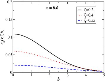
(a)    (b)

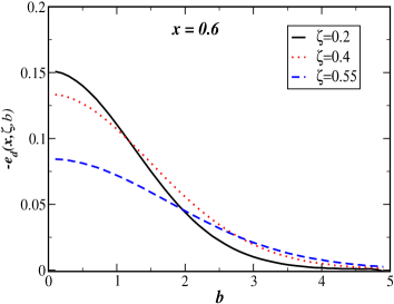
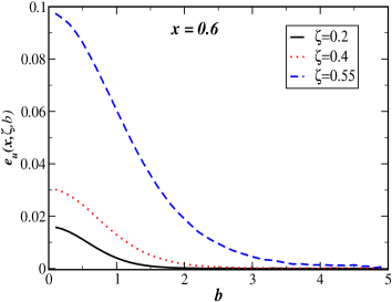
(c)   (d)

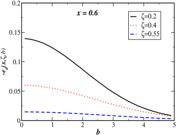
Figure 1: (Color online) Plots of (a) $e_{u}(x,\zeta,b)$ vs $b=\mid b_{\perp}\mid$ for fixed values of $x$ and $\zeta$ and for parameters as in set I (b) same as in (a) but for $d$ quark, (c) same as in (a) but the parameters are as in set II, (d) same as in (b) but the parameters are as in set II. $b$ is in GeV^-1.

As described in the introduction the ipdpdfs describe the probability of finding a parton of definite momentum fraction $x$ at a distance $b_{\perp}$ from the center of the proton. When the skewness $\zeta$ is nonzero, the transverse location of the proton itself is different before and after the scattering. This transverse shift does not depend on $x$ but on the skewness $\zeta$ and $b=\mid b_{\perp}\mid$. The information on the transverse shift is not washed out even if the GPDs are integrated over $x$ in the DVCS amplitude. In the DGLAP region $x>\zeta$, the impact parameter $b_{\perp}$ gives the location where the quark is pulled out and put back to the nucleon. In the ERBL region $\zeta<x$, $b_{\perp}$ denotes the transverse location of the quark-antiquark pair inside the nucleon. For a single fermion, the impact parameter dependent pdf would be a delta function. The smearing in $b_{\perp}$ space is due to the multiparticle correlation. In Fig. 1 we plot $e_{u}(x,\zeta,b)$ and $e_{d}(x,\zeta,b)$ as a function of $b$ for a fixed value of $x$ and different values of $\zeta$. Substantial difference is seen in the impact parameter space for the two sets of parametrization, set I and set II. In set I both $e_{u}$ and $e_{d}$ become more sharply peaked at $b=0$ when $\zeta$ is smaller. It is to be noted that the change in $e(x,b)$ with $b$ is related to the deformation of the parton distribution in impact parameter space for transversely polarized nucleon. For non-zero $\zeta$, this probes the deformation when the nucleon has a transverse shift before and after scattering. In set II for $e_{u}$, the peak increases as $\zeta$ increases, in contrast to set I, whereas for $e_{d}$, the peak decreases for increasing $\zeta$ but does not become broader as in set I.

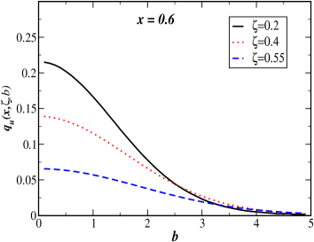
(a)    (b)

(c)   (d)

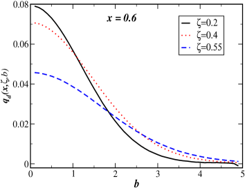
Figure 2: (Color online) Plots of (a) $q_{u}(x,\zeta,b)$ vs $b=\mid b_{\perp}\mid$ for fixed values of $x$ and $\zeta$ and for parameters as in set I, (b) same as in (a) but for $d$ quark, (c) same as in (a) but the parameters are as in set II, (d) same as in (b) but for parameters as in set II. $b$ is in GeV^-1.

In Fig. 2, we have plotted $q(x,\zeta,b)$ as a function of $b$ for fixed $x=0.6$ and different values of $\zeta$. As the two parametrizations set I and II are not much different for the GPD $H(x,\zeta,t)$ not much difference is seen in the impact parameter space. In all cases here the peak in $q(x,\zeta,b)$ for fixed $x$ decreases with increase of $\zeta$. For d quark distributions, the peak also becomes broader as $\zeta$ increases, which is the same behaviour as seen in $e(x,\zeta,b)$. As $\zeta$ increases for fixed $x$, the smearing in $b$ space becomes broader, which means that as the momentum transfer in the longitudinal direction increases, the active quark is more likely to be pulled out at a larger $b$.

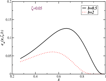
(a)    (b)

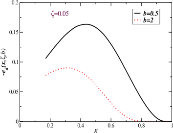
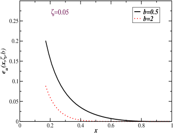
(c)   (d)

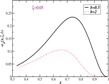
Figure 3: (Color online) Plots of (a) $e_{u}(x,\zeta,b)$ vs $x$ for fixed values of $b$ and $\zeta$ and for parameters as in set I, (b) same as in (a) but for $d$ quark, (c) same as in (a) but for parameters as in set II, (d) same as in (b) but for parameters as in set II. $b$ is in GeV^-1.

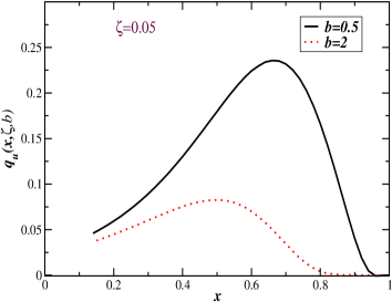
(a)    (b)

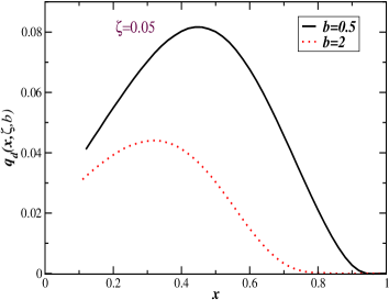
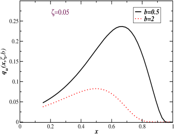
(c)   (d)

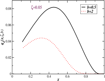
Figure 4: (Color online) Plots of (a) $q_{u}(x,\zeta,b)$ vs $x$ for fixed values of $b$ and $\zeta$ and for parameters as in set I, (b) same as in (a) but for $d$ quark, (c) same as in (a) but for parameters as in set II, (d) same as in (b) but for parameters as in set II. $b$ is in GeV^-1.

In Figs. 3 and 4 we plotted the impact parameter dependent distributions $e(x,\zeta,b)$ and $q(x,\zeta,b)$ for fixed $\zeta$ and $b$ values as functions of $x$. Substantial difference is observed in $e(x,\zeta,b)$ between set I and II, in particular in the low $x$ region. For $e_{u}$ the peak shifts towards smaller $x$ values ($x>\zeta$ in our calculation). However for $-e_{d}$ the peak shifts to higher $x$ values in set II. The qualitative behaviour of $q_{u}$ and $q_{d}$ are the same as functions of $x$.

The boost invariant longitudinal impact parameter $\sigma$ was first introduced in hadron_optics and it was shown that DVCS amplitude shows interesting diffraction pattern in longitudinal impact parameter space. GPDs also when expressed in term of $\sigma$ exhibit the similar diffraction pattern us2 . The boost invariant longitudinal impact parameter conjugate to the longitudinal momentum transfer is defined as $\sigma=\frac{1}{2}b^{-}P^{+}$. So, the GPDs in longitudinal position space is given by:

$$q(x,\sigma,t) = \frac{1}{2\pi}\int_{0}^{\zeta_{f}}d\zeta e^{i\zeta P^{+}b^{-}/2}H(x,\zeta,t)$$

$$= \frac{1}{2\pi}\int_{0}^{\zeta_{f}}d\zeta e^{i\zeta\sigma}H(x,\zeta,t)$$

$$e(x,\sigma,t) = \frac{1}{2\pi}\int_{0}^{\zeta_{f}}d\zeta e^{i\zeta P^{+}b^{-}/2}E(x,\zeta,t)$$ (13)

$$= \frac{1}{2\pi}\int_{0}^{\zeta_{f}}d\zeta e^{i\zeta\sigma}E(x,\zeta,t)$$

Since we are concentrating only in the region $\zeta<x<1$, the upper limit of $\zeta$ integration $\zeta_{f}$ is given by $\zeta_{max}$ if $x$ is larger then $\zeta_{max}$, otherwise by $x$ if $x$ is smaller than $\zeta_{max}$ where $\zeta_{max}$ is the maximum value of $\zeta$ allowed for a fixed $-t$:

$$\zeta_{max}={(-t)\over 2M^{2}}\Big{(}\sqrt{1+{4M^{2}\over(-t)}}-1\Big{)}.$$ (14)

In Figs. 5 and 6 we have plotted the GPDs in longitudinal position space $\sigma$. We restrict ourselves to the DGLAP region. The GPDs show diffraction pattern in $\sigma$ space, similar to that observed for a dressed electron in QED or in a holographic model for the meson hadron_optics . There is a primary maximum followed by a series of secondary maxima. The positions of the minima are the same for both u and d quark GPDs and they do not depend whether we are plotting $q(x,\sigma,b)$ or $e(x,\sigma,b)$. The feature was also observed for a dressed electron state in hadron_optics . The positions of the minima are characteristics of the finite Fourier transform and independent of the GPD used. As $-t$ increases, the positions of the first minima move in to smaller values of $\sigma$. As seen in Fig. 5, for set II, the peaks in $e_{u}(x,\sigma,t)$ are more sharp compared to set I. On the other hand, for $e_{d}(x,\sigma,t)$ the magnitude of the peak is more affected as $-t$ increases in set II compared to set I. However for $q_{u}(x,\sigma,t)$ and $q_{d}(x,\sigma,t)$ there is not much difference between the two parametrization sets, as expected. In all cases, the magnitude of the peak decreases as $-t$ increases and the first minima move in. This effect has already been observed for a dressed electron state and in a holographic model for the meson hadron_optics ; as well as for chiral odd GPDs us2 . In hadron_optics a relation between the position of the first minima and the momentum transfer squared $-t$ has been derived in analogy with diffraction in optics. The fact that such pattern with the same qualitative behaviour is observed here in a phenomenological parametrization of GPDs shows that it is not an artefact of the cuts and constraints used in the field theory based model. In pion pion distribution amplitudes (DAs) have been investigated in longitudinal position space (Ioffe time) by expressing the DAs in an expansion over Gegenbauer polynomials. Oscillation of the DA has been observed in longitudinal position space showing two humps in certain models. It was concluded that this is an artefact of truncating the conformal spin partial wave expansion. In order to further investigate the diffraction pattern that we observe for the GPDs, in Fig. 7 we plot the GPD $H$ in longitudinal position space using a model similar to that in marc . For the dotted and long dashed curves we chose a factorized ansatz of the form

$$H(x,\zeta,t)=Nu(x)F_{1}(t)$$ (15)

where $N$ is the normalization constant, we took $u(x)=x(1-x)$ and for the form factor $F_{1}(t)$ we took the standard dipole form. The FT shows diffraction pattern with the general features the same as observed in other models. In the solid and short-dashed curves, we used a somewhat different ansatz, namely

$$H(x,\zeta,t)={\cal{N}}u(x,\zeta)F_{1}(t)$$ (16)

where we took the same dipole form factor, and $u(x,\zeta)=(x-\zeta)^{2}(1-x)^{2}$; ${\cal{N}}$ being the normalization constant. The normalization constants have been chosen to fit the two sets of curves in the same plot. There is no diffraction pattern in the second model; which clearly shows that the pattern is not only due to the finite range of the $\zeta$ integration but depends also on the $x,\zeta$ and $t$ interplay in the GPD parametrization used. So an experimental observation of such diffraction pattern can help to constrain GPD parametrizations. However in order to get the full Lorentz invariant picture in longitudinal position space one has to consider the other kinematical region $x<\zeta$ as well; as explained in hadron_optics . Also the positions of the minima and their shift with increase of $-t$ are model independent features of the Fourier transform.

IV Conclusion

In this work we investigated the GPD for u and d quark distributions in the proton using a recent parametrization liuti2 . For nonzero $\zeta$ we worked in the DGLAP region $x>\zeta$. Taking a Fourier transform with respect to the transverse momentum transfer $\Delta_{\perp}$ we obtained the parton distributions in impact parameter space. For nonzero $\zeta$ these probe the parton distributions when the initial proton is shifted from the final proton in the transverse plane. When the proton is transversely polarized, the parton distributions in the tranverse plane is distorted, this distortion is related to the GPD $E(x,\zeta,t)$ and to the orbital angular momentum of the quarks. We showed the $x$ and $b_{\perp}$ dependence of the ipdpdfs for various $\zeta$ values. We introduced a boost invariant longitudinal impact parameter $\sigma$ conjugate to $\zeta$. Both the GPDs $H$ and $E$ in $\sigma$ space show diffraction pattern as seen before in some other models. We did some comparative study using different toy models and showed that although the general features of this pattern are independent of specific models but the appearance of the diffraction pattern depends not only on the finiteness of the $\zeta$ integration but also on the interplay of the $x$, $\zeta$ and $t$ dependence of the GPDs.

V Ackowledgement:

AM thanks DST fasttrack scheme, Govt. of India, for support.

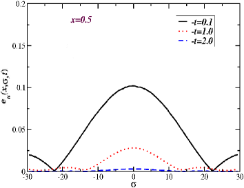
(a)    (b)

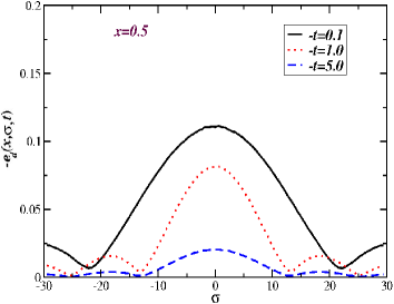
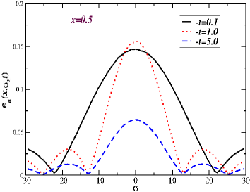
(c)   (d)

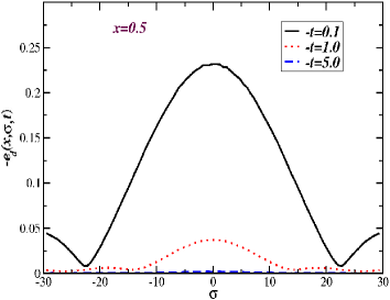
Figure 5: (Color online) Plots of (a) $e_{u}(x,\sigma,t)$ vs $\sigma$ , (b) $-e_{d}(x,\sigma,t)$ vs $\sigma$ for a fixed value of $x$ with different $-t$ in GeV². (c) same as (a) and (d) same as (b) but for the second parametrization.

(a)    (b)

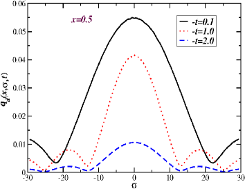
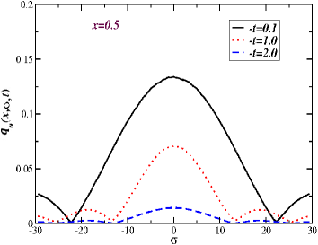
(c)   (d)

Figure 6: (Color online) Plots of (a) $q_{u}(x,\sigma,t)$ vs $\sigma$ , (b) $q_{d}(x,\sigma,t)$ vs $\sigma$ for fixed values of $x$ and different $-t$ in GeV². (c) same as (a) and (d) same as (b) but for the second parametrization.

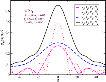
Figure 7: (Color online) Plots of $q_{u}(x,\sigma,t)$ in the model given by Eq. (15) (dotted and long dashed) and Eq. (16) (solid and short dashed)

References

- (1) For reviews on generalized parton distributions, and DVCS, see M. Diehl, Phys. Rept, 388, 41 (2003); A. V. Belitsky and A. V. Radyushkin, Phys. Rept. 418 1, (2005); K. Goeke, M. V. Polyakov, M. Vanderhaeghen, Prog. Part. Nucl. Phys. 47, 401 (2001).
- (2) C. Adloff et. al., (H1 Collaboration), Eur. Phys. J. C 13, 371 (2000).
- (3) C. Adloff et. al. (H1 Collaboration), Phys. Lett. B 517, 47 (2001).
- (4) J. Breitweg et. al. (ZEUS Collaboration), Eur. Phy. J. C 6, 603 (1999).
- (5) S. Chekanov et. al. (ZEUS Collaboration), Phys. Lett. B 573, 46 (2003).
- (6) A. Airapetian et. al. (HERMES Collaboration), Phys. Rev. Lett. 87, 182001 (2001).
- (7) S. Stepanyan et. al. (CLAS Collaboration), Phys. Rev. Lett. 87, 182002 (2001).
- (8) N. D’Hose, E. Burtin, P. A. M. Guichon, J. Marroncle (COMPASS Collaboration), Eur. Phys. J. A 19, 47 (2004).
- (9) S. Boffi, B. Pasquini, Riv.Nuovo Cim.30:387,2007.
- (10) M. Burkardt, Int. J. Mod. Phys. A 18, 173 (2003); M. Burkardt, Phys. Rev. D 62, 071503 (2000), Erratum- ibid, D 66, 119903 (2002); J. P. Ralston and B. Pire, Phys. Rev. D 66, 111501 (2002).
- (11) D. E. Soper, Phys. Rev. D 15, 1141 (1977).
- (12) M. Diehl, T. Feldman, R. Jacob, P. Kroll, Eur. Phys. J. C 39, 1 (2005).
- (13) M. Burkardt, Phys. Rev. D 72, 094020 (2005).
- (14) S. Meissner, A. Metz and K. Goeke,Phy. Rev. D 76, 034002 (2007).
- (15) X. Ji, Phy. Rev. Lett. 91, 062001 (2003); A. Belitsky, X. Ji, F. Yuan, Phys. Rev. D 69 074014 (2006).
- (16) S. Meissner, A. Metz, M. Schegel, JHEP08, 056 (2009).
- (17) S. J. Brodsky, D. Chakrabarti, A. Harindranath, A. Mukherjee and J. P. Vary, Phys. Lett. B 641, 440 (2006); Phys. Rev. D 75, 014003 (2007).
- (18) S. Ahmad, H. Honkanen, S. Liuti, S. Taneja, Eur. Phys. J. C 63, 407 (2009).
- (19) S. Ahmad, H. Honkanen, S. Liuti and S. Taneja, Phys. Rev. D 75, 094003 (2007).
- (20) S. J. Brodsky, M. Diehl, D. S. Hwang, Nucl. Phys. B 596, 99 (2001).
- (21) D. Chakrabarti and A. Mukherjee, Phys. Rev. D 71, 014038 (2005); Phys. Rev. D 72, 034013 (2005); A. Mukherjee and M. Vanderhaeghen, Phys. Lett. B 542, 245; Phys. Rev. D 67, 085020 (2003).
- (22) K. Kumericki, D. Muller, arXiv:0904.0458 [hep-ph].
- (23) D. Chakrabarti, R. Manohar and A. Mukherjee, Phys. Lett. B 682, 428 (2010).
- (24) S. Alekhin, Phys. Rev. D 68, 014002 (2003).
- (25) D. Chakrabarti, R. Manohar and A. Mukherjee, Phys. Rev. D 79, 034006 (2009).
- (26) V. Braun, D. Mueller, Eur. Phys. J. C 55, 349 (2008).
- (27) M. Guidal, M. V. Polyakov, A. V. Radyushkin, M. Vanderhaeghen, Phys. Rev. D 72, 054013 (2005).
(a) (b)
(b)
(c) (d)
(d)
(a) (b)
(b)
(c) (d)
(d)
(a) (b)
(b)
(c) (d)
(d)
(a) (b)
(b)
(c) (d)
(d)
(a) (b)
(b)
(c) (d)
(d)
(a) (b)
(b)
(c) (d)
(d)