The LBA Calibrator Survey of southern compact extragalactic radio sources — LCS1

Abstract

We present a catalogue of accurate positions and correlated flux densities for 410 flat-spectrum, compact extragalactic radio sources previously detected in the AT20G survey. The catalogue spans the declination range $[-90\degr,-40\degr]$ and was constructed from four 24-hour VLBI observing sessions with the Australian Long Baseline Array at 8.3 GHz. The VLBI detection rate in these experiments is 97%, the median uncertainty of the source positions is 2.6 mas, and the median correlated flux density on projected baselines longer than 1000 km is 0.14 Jy. The goals of this work are 1) to provide a pool of southern sources with positions accurate to a few milliarcsec, which can be used for phase referencing observations, geodetic VLBI and space navigation; 2) to extend the complete flux-limited sample of compact extragalactic sources to the southern hemisphere; and 3) to investigate the parsec-scale properties of high-frequency selected sources from the AT20G survey. As a result of this VLBI campaign, the number of compact radio sources south of declination $-40\degr$ which have measured VLBI correlated flux densities and positions known to milliarcsec accuracy has increased by a factor of 3.5. The catalogue and supporting material is available at http://astrogeo.org/lcs1.

1 Introduction

Catalogues of positions of compact extragalactic radio sources with the highest accuracy are important for many applications. These include imaging faint radio sources in the phase referencing mode, differential astrometry, space geodesy, and space navigation. The method of VLBI first proposed by Matveenko, Kardashev & Sholomitskii (1965) allows us to derive the position of sources with nanoradian precision (1 nrad $\approx$ 0.2 mas). The first catalogue of source coordinates determined with VLBI contained 35 objects (Cohen & Shaffer, 1971). Since then hundreds of sources have been observed under geodesy and astrometry VLBI observing programs at 8.6 and 2.3 GHz (X and S bands) using the Mark3 recording system at the International VLBI Service for Geodesy and Astrometry (IVS) network. Analysis of these observations resulted in the ICRF catalogue of 608 sources (Ma et al., 1998).

The Very Long Baseline Array (VLBA) was later used to measure the positions of $~{}\!4000$ compact radio sources in the VLBA Calibrator Survey (VCS) (Beasley et al., 2002; Fomalont et al., 2003; Petrov et al., 2005, 2006; Kovalev et al., 2007; Petrov et al., 2007a) and the geodetic program RDV (Petrov et al., 2009b). All sources with declinations above $-45\degr$ detected using Mark3/Mark4 under IVS programs were re-observed with the VLBA in the VCS and RDV programs, which significantly improved the accuracy of their positions. As a result of these efforts, the probability of finding a calibrator with a VLBI-determined position greatly increased. In the declination range $\delta>-30\degr$ the probability of finding a calibrator within a $3\degr$ radius of a given position reached 97% by 2008.

Since the VLBA is located in the northern hemisphere, observations in the declination zone $[-50\degr,-30\degr]$ are difficult and the array cannot observe sources with $\delta<-52\degr$. In 2008, the probability of finding a calibrator within a radius of $3^{\circ}$ was 75% in the declination zone $[-40^{\circ},-30^{\circ}]$ and 42% for declinations south of $-40^{\circ}$. The VLBI calibrator list in 2008 had 524 sources in the zone $[+52^{\circ},+90^{\circ}]$, but only 98 objects in the zone $[-52^{\circ},-90^{\circ}]$ which cannot be reached by the VLBA. These southern sources were observed during geodetic experiments and during two dedicated southern hemisphere astrometry campaigns (Fey et al., 2004, 2006). The reason for this disparity is the scarcity of VLBI antennas in the southern hemisphere, particularly stations with dual frequency S/X receivers and geodetic recording systems. Also until recently there has been a lack of good all-sky catalogues suitable for finding candidate VLBI calibrators.

The Australian Long Baseline Array (LBA) consists of six antennas located in Australia with the South Africa station hartrao often joining in. This VLBI network operates 3–4 observing sessions a year, each about one week long. Although the hardware used by the LBA was not designed for geodesy and absolute astrometry observations, it was demonstrated by Petrov et al. (2009a) that despite significant technical challenges, absolute astrometry VLBI observations with the LBA network is feasible. In a pilot experiment in June 2007, the positions of participating stations were determined with accuracies 3–30 mm, and positions of five new sources were determined with accuracies 2–5 mas.

Inspired by these astrometric results, we launched the X-band LBA Calibrator Survey observing campaign (LCS), with the aim of determining milliarcsecond positions and correlated flux densities for one thousand compact extragalactic radio sources at declinations south of $-30^{\circ}$. The overall objective of this campaign is to match the density of calibrators in the northern hemisphere and so eliminate the disparity.

We have three long-term goals in this campaign. Firstly, setting up a dense grid of calibrators with precisely known positions within several degrees of any target will make make phase-referencing observations of weak targets feasible. According to Wrobel (2009), 63% of VLBA observations in 2003–2008 were made in the phase referencing mode. A dense grid of calibrators also makes it possible to do differential astrometry of Galactic objects such as pulsars and masers, and allows direct determination of the parallax at distances up to several kiloparsec (Deller et al., 2009). These sources form the pools of targets for observations under the geodesy programs and for space navigation.

Our second goal is to extend the complete flux-limited sample of compact extragalactic radio sources (with emission from milliarcsecond-size regions) to the entire sky. According to Kovalev (private communication, 2010), analysis of the $\log N$–$\log S$ diagram of the VLBI calibrator list suggests the sample of radio–loud Active Galactic Nuclei (AGN) is complete at the level of correlated flux density 200 mJy at X-band at spatial frequencies 25 $M\lambda$ at $\delta>-30\degr$. Extending this complete sample to the entire sky will make it possible to generalize the properties of the sample, such as distribution of compactness, distribution of brightness temperature, bulk motion, viewing angle, irregularities of the spatial distribution, to the entire population of radio loud AGN.

The third goal is to investigate the properties of high-frequency selected radio sources from the Australia Telescope 20 GHz (AT20G) survey (Murphy et al., 2010; Massardi et al., 2010). Obtaining observations of a subsample of AT20G sources with milliarcsecond resolution will allow us to investigate the properties, such as spectral index, polarization fraction and variability, of a population of extremely compact sources.

In this paper, we present the results from the first four 24-hour experiments observed in 2008–2009. The selection of candidate sources from the AT20G catalogue is discussed in section 2. The station setups during the observing sessions is described in section 3. The correlation and post-correlation analysis, which is rather different from ordinary VLBI experiments, is discussed in sections 4 and 5. An error analysis of single-band observations, including evaluation of ionosphere-driven systematic errors, is given in subsection 5.2. The catalogue of source positions and correlated flux densities is presented in section 6, and the results are summarized in section 7.

2 Candidate source selection

The Australia Telescope 20 GHz (AT20G) survey is a blind radio survey carried out at 20 GHz with the Australia Telescope Compact Array (ATCA) between 2004 and 2008 (Murphy et al., 2010). It covers the whole sky south of declination 0°. The source catalogue is an order of magnitude larger than previous catalogues of high-frequency radio sources, with 5890 sources above a 20 GHz flux-density limit of 40 mJy. All AT20G sources have total intensity and polarization measured at 20 GHz, and most sources south of declination $-15\degr$ also have near-simultaneous flux-density measurements at 4.8 and 8.6 GHz. A total of 1559 sources were detected in polarised total intensity at one or more of the three frequencies. There are also optical identifications and redshifts for a significant fraction of the catalogue.

This high-frequency catalogue provides a good starting point for selecting bright, compact sources and candidate calibrators. Massardi et al. (2010) show that almost all the flat-spectrum AT20G sources with spectral index $\alpha>-0.5$ are unresolved on scales of 0.1–0.2 arcsec in size at 20 GHz (see their fig. 3.4). The few exceptions are either (i) foreground Galactic and LMC sources such as planetary nebulae, HII regions and pulsar wind nebulae, which have a flat radio spectrum due to their thermal emission but are usually resolved on scales of a few arcsec (Murphy et al., 2010), or (ii) flat-spectrum extragalactic sources which are gravitationally-lensed, like PKS 1830$-$211.

For 64% of sources from the AT20G catalogue, flux densities were determined in three bands, 5.0, 8.4 and 20 GHz. We used these measurements to calculate the spectral index $\alpha$ ($F\propto f^{\alpha}$). We selected a set of 684 objects, not previously observed with VLBI, which had a flux density $>150$ mJy at 8.3 GHz and a spectral index $>-0.6$. We then split this sample into two subsets: 410 high priority sources with flux densities $>200$ mJy and spectral indices $>-0.5$, and all others. In addition, we selected 14 flat-spectrum objects that did not have flux density measurements at 5 GHz and 8 GHz in AT20G. Their spectral indices were determined by analyzing historical single dish observations found in the Astrophysical CATalogs support System CATS (Verkhodanov et al., 1997) database, which by 2010 included data from 395 catalogues from radioastronomy surveys.

In addition to these target sources, we identified a set of 195 sources that we used for calibrator selection. These were bright sources previously observed at the VLBA or IVS network with position known with accuracies better 0.5 mas and with correlated flux densities $>500$ mJy on baselines longer than 5000 km.

2.1 The Long Baseline Array

The LBA network used for LCS1 consists of 6 stations: atca-104, ceduna, dss45, hobart26, mopra and parkes (Fig. 1, Table 1). The maximum baseline length of the network is 1703 km, the maximum equatorial baseline projection is 1501 km, and the maximum polar baseline projection is 963 km.

Table 1: The LBA network stations. The average System Equivalent Flux Density (SEFD) at 8.3 GHz at elevation angles $>60\degr$ achieved in LCS1 experiments is shown in the last column.

Name	$\phi_{gc}$	$\lambda$	Diam	SEFD
atca-104	-$30\degr.15$	$149\degr.57$	22 m	350 Jy
ceduna	-$31\degr.70$	$133\degr.81$	32 m	490 Jy
dss45	-$35\degr.22$	$148\degr.98$	34 m	120 Jy
hobart26	-$42\degr.62$	$147\degr.44$	26 m	620 Jy
mopra	-$31\degr.10$	$149\degr.10$	22 m	380 Jy
parkes	-$32\degr.82$	$148\degr.26$	64 m	36 Jy

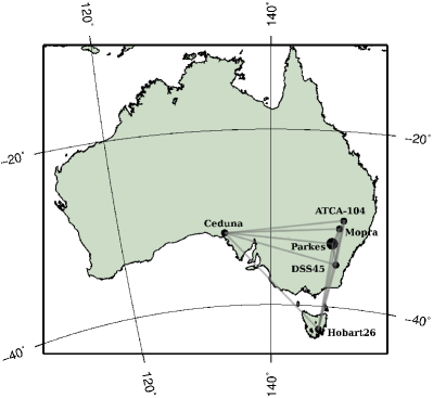
Figure 1: The LBA network used for LCS1 observations.

2.2 Observation scheduling

Observation schedules were prepared with the software program sur_sked. The scheduling goal was to observe each target source with all antennas of the array in three scans of 120 seconds each in the first three experiments and in four scans in the last experiment. After tracking a target source for 120 seconds, each antenna immediately slewed to the next object. The minimum time interval between consecutive scans of the same source was 3 hours. The scheduling software computed the elevation and azimuth of each candidate source, with constraints on the horizon mask and maximum elevations to which antennas can point. It calculated the slewing time taking into account the antenna slewing rate, slewing acceleration and cable wrap constraints. The sources were scheduled to minimize slewing time and fit the scheduling constraints. A score was assigned for each target source visible at a given time, depending on the slewing time, the history of past observations in the experiment and the amount of time that the source would remain visible to all antennas in the array.

Every hour a set of four calibrator sources was observed: two scans where all antennas had an elevation in the range $[12\degr,45\degr]$, one scan at elevations $[32\degr,45\degr]$ and one scan at elevations $[45\degr,90\degr]$. Scans with calibrator sources were 70 seconds long. The scheduling algorithm for each set found all combinations of calibrator sources that fell in the right elevation range, and selected the sequence of four objects that minimized the slewing time. The purpose of these observations was 1) to serve as amplitude and bandpass calibrators; 2) to improve the robustness of estimates of the path delay in the neutral atmosphere; and 3) to tie the positions of new sources to existing catalogues such as the ICRF catalogue (Ma et al., 1998).

The scheduling algorithm assigned four scans for 18% of target sources, three scans for 76% of sources, two scans for 3% of sources, and one scan for 3% of sources. Of the 26 targets with fewer than three scans in a given observing session, 18 were observed in two experiments. During a 24 hour experiment, 11.5–12.0 hours were used for observing target sources, 1.5–2.0 hours for observing calibrators.

3 Observations

Table 2: Observation Summary for each observing session

Telescope	Recorder	Polarization	Frequency Bands (MHz)
Experiment v254b, February 05 2008
parkes atca-104 mopra hobart26 ceduna	LBADR	RCP only	8256–8272 8272–8288 8512–8528 8528–8544
Experiment v271a, August 10 2008
parkes hobart26 dss45	Mark5	RCP only	8200–8216 8216–8232 8232–8248 8248–8264 8456–8472 8472–8488 8488–8504 8504–8520
ceduna	LBADR	RCP only	8200–8216 8216–8232 8456–8472 8472–8488
atca-104 mopra	LBADR	RCP & LCP	8200–8216 8216–8232 8456–8472 8472–8488
Experiment v271b, November 28 2008
parkes hobart26 dss45	Mark5	RCP only	8200–8216 8216–8232 8264–8280 8328–8344 8392–8408 8456–8472 8472–8488 8520–8536
ceduna	LBADR	RCP only	8200–8216 8216–8232 8456–8472 8472–8488
atca-104 mopra	LBADR	RCP & LCP	8200–8216 8216–8232 8456–8472 8472–8488
Experiment v271c, July 04 2009
hobart26	Mark5	RCP only	8200–8216 8216–8232 8232–8248 8328–8344 8344–8360 8456–8472 8472–8488 8488–8504
parkes	Mark5 & LBADR	RCP & LCP	8200–8216 8216–8232 8232–8248 8328–8344 8344–8360 8456–8472 8472–8488 8488–8504
ceduna	LBADR	RCP only	8200–8216 8216–8232 8456–8472 8472–8488
atca-104 mopra	LBADR	RCP & LCP	8200–8216 8216–8232 8456–8472 8472–8488

As mentioned in the introduction, not all of the telescopes in the LBA network are capable of observing in the typical geodetic/astrometric mode of dual S/X frequency bands with multiple spaced subbands and recorded to a Mark5 VLBI system.

The hobart26, parkes, and dss45 have a Mark5 recording system and a Mark4 (Whitney et al., 2004) baseband conversion rack. However for the first epoch the LBADR system (Phillips et al., 2009) was used. For all subsequent experiments the Mark5 system was used. Data were recorded onto normal Mark5 diskpacks and shipped to the Max-Plank Institut für Radioastronomie in Bonn for processing.

The atca-104, mopra and ceduna only have the standard LBA VLBI backend consisting of an Australia Telescope National Facility (ATNF) Data Acquisition System (DAS) with an LBADR recorder. The ATNF DAS only allows two simultaneous intermediate frequencies (IFs): either 2 frequencies or 2 polarizations. For each of these IFs the input 64 MHz analog IF is digitally filtered to 2 contiguous 16 MHz bands. atca-104, mopra, and parkes have two ATNF DAS, however the IF conversion system at each telescope means it is impractical to run in any modes other than 2 frequencies and dual polarization. The LBADR data format is not compatible with the Mark4 data processor at Bonn. A custom program was written to translate the data to Mark5B format then it was electronically copied using the Tsunami-UDP application to Bonn, before being copied onto Mark5 diskpacks.

In the last experiment parkes recorded on the LBADR system in parallel with the Mark5. As this included left circular polarization (LCP) which was not recorded on the Mark5 system and since atca-104 and mopra recorded both RCP and LCP, the LBADR data were also sent to Bonn and LCP correlated against atca-104 and mopra.

The main limiting factor for frequency selection was the LBADR backend at atca-104, mopra and ceduna where a setup with bands centered on $\sim$8.2 and$\sim$8.5 GHz was chosen. For the telescopes with Mark5 recorders, the setup was chosen to overlap in frequency with the LBADR setup but also including more frequencies to gain sensitivity. The frequency setup was changed between experiments in order to explore the feasibility of recording at 512 Mbit/s at those stations that can support it. The setup for each observing experiment is described in Table 2.

The Australia Telescope Compact Array consists of six 22 metre antennas and may observe as a single antenna or as a phased array of 5 dishes. Since no tests of using a phased ATCA array as an element of the VLBI network for absolute astrometry observations were made before 2010, we decided to use a single dish of the ATCA in order to avoid the risk of introducing unknown systematic errors.

The NASA Deep Space Network station dss45 observed only 4.5 hours in v271a and 6.5 hours in v271b during intermissions between receiving the telemetry from Mars orbiting spacecraft.

4 Correlation

The Bonn Mark4 Correlator was chosen for the correlation of these experiments for two primary reasons. Firstly, the correlator was extensively tested for use in space geodesy and absolute astrometry mode during 2000–2010 and is known to produce highly reliable group delays. Secondly, it was equipped with four Mark5B units and eight Mark5A units, which was a convenient combination since data from parkes were recorded in the Mark5B format and data from atca-104, mopra, and cedunaoriginally recorded in LBADR format were transformed to the Mark5B format before correlation.

Preparation for correlation required about two months due to complications that arose from the scheduling of different patching and channel outputs (fan out) for use at the stations. The stations that had Mark4 data acquisition racks delivered detailed log files, from which we could reconstruct the channels used, but the LBA stations did not provide log files and the track assignments had to be searched for by trial and error, which was a time-consuming process. The absence of log files also required some custom programming to reconstruct the log VEX file (lvex), which the Mark IV correlator required to perform the correlation. Further, the setup that was chosen was incompatible with the capabilities of the hardware correlator and required an extensive work-around at the correlator.

We chose to correlate with a window of 128 lags (corresponding to a delay window width of 8 $\mu$s) instead of the 32 lags (2 $\mu$s) normally used for stream correlation. This was to allow for potentially large clock offsets due to instrumental errors, and for large a priori source coordinate errors. The integration time was chosen to be as small as possible (0.5 s to 1.0 s) to allow for potentially large residual fringe rates due to source position errors.

The Mark4 correlator can cope with only four stations simultaneously when correlating 128 lags with short integration time. Since the experiment was observed with five to seven stations in right circular polarization (RCP) and two stations (atca-104 and mopra) also in left circular polarization (LCP), the correlation had to be split in passes.

As a by-product of the multi-pass correlation, some baselines were correlated more than once and this redundancy was exploited to select the correlation with the best SNR for each duplicated scan. For the LCP correlation, only one pass was required since only the LBA stations recorded LCP. parkes recorded LCP only during v271c and this was enabled by the use of two backends (Mark4 and LBA) in parallel. Those stations were re-correlated in a second pass to produce all four polarization products (left-left, right-right, left-right and right-left). For this pass we had to restrict the number of lags to 32 due to correlator hardware constraints, but the integration time was kept at 0.5 s.

Fringe fitting was performed at the correlator using software program fourfit, the baseline-based fringe fit offered within the Haystack Observatory Package Software (hops) to estimate the residual delay upon which the post-correlation analysis was based. Inspection of fringe-fitted data is a convenient means of data quality control, as one can examine the correlated data on a scan-by-scan basis, looking for problems that might have occurred during correlation or at the stations and permits flagging of bad data immediately.

5 Data analysis

The correlator either generates the spectrum of the cross-correlation function directly, or it can be easily derived from its raw output. The spectrum was processed with the software program fourfit, which for each scan and each baseline determined the phase delay rate, narrow-band delay and wide-band group delay (sometimes also called multi-band delay) that maximized the fringe amplitude. Takahashi et al. (2000) give a detailed description of the fringe searching process and the distinction between narrow-band and wide-band group delays. The wide-band delay is more precise than narrow-band delay. The formal uncertainties of these delays, $\sigma_{n}$ and $\sigma_{w}$ are computed by fourfit the following way:

$$\begin{array}[]{lcl}\sigma_{n}&=&\frac{\displaystyle\sqrt{12}}{\displaystyle 2\pi\Delta f\>{\mbox{\rm SNR}}}\\ \sigma_{w}&=&\frac{\displaystyle 1}{\displaystyle 2\pi\sigma_{f}\>{\mbox{\rm SNR}}},\end{array}$$ (3)

where $\Delta f$ the IF bandwidth, $\sigma_{f}$ the dispersions of cyclic frequencies across the band, and SNR is the ratio of the fringe amplitude from the wide band fringe search to the rms of the thermal noise. The ratio of $\sigma_{w}/\sigma_{n}$ was in the range 27–28 for the LCS1 experiments, which gives for observations with typical SNR=30 $\sigma_{w}\approx 40$ ps and $\sigma_{n}$ around one nanosecond.

Of the 421 observed targets, 410 were detected. The list of 11 undetected sources is given in Table 3. In addition 111 calibrators were observed, all of which were detected.

Table 3: The list of target sources that were not detected in LCS1 VLBI observations. The last three data columns contain the flux density in mJy extrapolated to 8.3 GHz (F), the spectral index ($\alpha$), and comment (C). Value -9.99 means the spectral index was not available. Comments: 1) Not in AT20G catalogue; 2) Flagged as an LMC source in AT20G catalogue; 3) Galactic planetary nebula; 4) Flagged as an extended source in AT20G catalogue. The table is also available in the electronic attachment.

J2000-name	B1950	RA			Dec			F	$\alpha$	C
J0404$-$7109	0404$-$712	04	04	00.99	-71	09	09.7	172	-0.57	1
J0538$-$6905	0539$-$691	05	38	45.66	-69	05	03.1	204	-9.99	2
J0552$-$5349	0551$-$538	05	52	36.18	-53	49	32.4	182	-0.34	1
J0938$-$6005	0937$-$598	09	38	47.20	-60	05	28.7	196	-0.08	3
J0958$-$5757	0956$-$577	09	58	02.92	-57	57	42.6	383	0.21	3
J1100$-$6514	1058$-$649	11	00	20.09	-65	14	56.4	179	-0.08	3
J1150$-$5710	1147$-$569	11	50	17.87	-57	10	56.0	349	0.23	3
J1325$-$4302	1322$-$427	13	25	07.35	-43	02	01.8	327	-9.99	4
J1353$-$6630	1350$-$662	13	53	57.05	-66	30	50.3	370	0.04	3
J1505$-$5559	1502$-$557	15	05	59.17	-55	59	16.2	217	-0.06	3
J1656$-$4014	1653$-$401	16	56	47.53	-40	14	24.4	427	-9.99	4

5.1 Data analysis: source position determination

The most challenging part of data analysis was resolving group delay ambiguities. The algorithm for fringe fitting implemented in fourfit searches for a global maximum in the Fourier transform of the cross-correlated function, averaged over individual IFs after correcting phases for a fringe delay rate and a narrow-band group delay. Fringe spectrum folding results in a rail of maxima of the Fourier transform of the cross-correlated function with exactly the same amplitude and with spacings reciprocal to the minimum difference in intermediate frequencies, $1/16.0\cdot 10^{6}\,\mbox{Hz}=62.5$ ns. Within one half of the 62.5 ns range, the fringe spectrum has several strong secondary maxima. The second maximum at $1/256.0\cdot 10^{8}\,\mbox{Hz}\approx 3.9$ ns has the amplitude 0.981 of the main maximum, the third maximum at $2/256.0\cdot 10^{8}\,\mbox{Hz}\approx 7.8$ ns has the amplitude 0.924. This high level of secondary maximum amplitudes is due to our choice of intermediate frequencies that was determined by the hardware limitations. Due to the presence of noise in the cross-correlated function, the difference between the fringe amplitude at the main maximum and at the secondary maxima is random, and therefore, the group delay is determined with an uncertainty $\pm 1-3$ of the spacing between the secondary maxima, 3.9 ns.

It should be noted that typical group delay ambiguity spacings in geodetic observations are in the range 50–200 ns. For successfully resolving ambiguities, as a rule of thumb the predicted delay should be known with an accuracy better than 1/6 of the ambiguity spacing, 600 ps in our case. This is a challenge. The random errors of the narrow-band group delays are too high to use directly for resolving ambiguities in wide-band group delays (see Fig. 2). In the framework of traditional data analysis of geodetic VLBI observations, the maximum uncertainty in prediction of the path delay is due to a lack of an adequate model for the path delay in the neutral atmosphere. These errors are in the range of 300–2000 ps. The path delay through the ionosphere at 8.3 GHz is in the range 30–1000 ps. In addition, an error $1^{\prime\prime}$ in a priori source position (a typical AT20G position error) causes an error in a priori time delay of up to 30 ns on a 1700 km baseline.

5.1.1 Group delay ambiguity resolution

However, it is premature to conclude that resolving group delay ambiguities is impossible. Firstly, we need to use a state-of-the art a priori model. Our computation of theoretical time delays in general follows the approach of Sovers, Fanselow & Jacobs C.S (1998) with some refinements. The most significant ones are the following. The advanced expression for time delay derived by Kopeikin & Schäfer (1999) in the framework of general relativity was used. The displacements caused by the Earth’s tides were computed using the numerical values of the generalized Love numbers presented by Mathews (2001) following a rigorous algorithm described by Petrov & Ma (2003) with a truncation at a level of 0.05 mm. The displacements caused by ocean loading were computed by convolving the Greens’ functions with ocean tide models. The GOT99.2 model of diurnal and semi-diurnal ocean tides (Ray, 1999), the NAO99 model (Matsumoto, Takanezawa & Ooe, 2000) of ocean zonal tides, the equilibrium model (Petrov & Ma, 2003) of the pole tide, and the tide with period of 18.6 years were used. Station displacements caused by the atmospheric pressure loading were computed by convolving the Greens’ functions that describe the elastic properties of the Earth (Farrell, 1972) with the output of the atmosphere NCEP Reanalysis numerical model (Kalnay et al., 1996). The algorithm of computations is described in full detail in Petrov & Boy (2004). The displacements due to loading caused by variations of soil moisture and snow cover in accordance with GLDAS Noah model (Rodell et al., 2004) with a resolution $0.25^{\circ}\times 0.25^{\circ}$ were computed using the same technique as the atmospheric pressure loading. The empirical model of harmonic variations in the Earth orientation parameters heo_20101111 derived from VLBI observations according to the method proposed by Petrov (2007) was used. The time series of UT1 and polar motion derived by the NASA Goddard Space Flight Center operational VLBI solutions were used a priori.

The a priori path delays in the neutral atmosphere in the direction of observed sources were computed by numerical integration of differential equations of wave propagation through the heterogeneous media. The four-dimensional field of the refractivity index distribution was computed using the atmospheric pressure, air temperature and specific humidity taken from the output of the Modern Era Retrospective-Analysis for Research and Applications (MERRA) (Schubert et al., 2008). That model presents the atmospheric parameters at a grid $1/2\degr\times 2/3\degr\times 6^{h}$ at 72 pressure levels.

Secondly, we made a least square (LSQ) solution using narrow-band delay. The positions of all target sources were estimated, as well as clock functions for all stations except the one taken as a reference and the residual atmosphere path delay in zenith directions. The clock function was modeled as a sum of the 2nd degree polynomial over the experiment and B-spline of the first order with the time span 60 minutes. The residual atmosphere path delay in zenith direction was modeled with B-spline of the first order with time span 60 minutes. Constraints on rate of change of clock function and atmosphere path delay were imposed. After the removal of outliers (1–2% of points), the weighted root mean square (wrms) of residuals was 1–4 ns. An example of narrow-band postfit residuals is shown in Fig. 2.

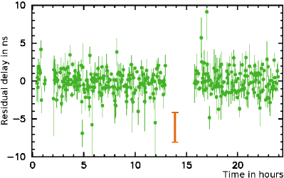
Figure 2: The post-fit residuals of narrow-band group delay LSQ solution at the baseline ceduna/hobart26 in experiment v271a on February 05, 2008. The bar in the middle of the plot corresponds to the ambiguity spacing of the wide-band path group delay.

The next step was to substitute the adjustments to clock function, atmosphere path delay in zenith direction and source positions from the narrow band LSQ solution to the differences between the wide-band path delays and the theoretical group delays. An example of enhanced wide-band group delays after the substitution and group delay ambiguity resolution is shown in Fig. 3.

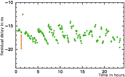
Figure 3: The wide-band a priori group delays after substitution of adjustments to clock function, atmosphere path delay in zenith direction and source positions from the narrow-band LSQ solution at the baseline ceduna/parkes in experiment v271a on February 05, 2008. The bar in the left side of the plot corresponds to the ambiguity spacing of the wide-band path group delay.

It is still difficult to resolve ambiguities at long baselines, but relatively easy to resolve the ambiguities at the inner part of the array: atca-104, dss45, mopra, parkes. The group delay ambiguity resolution process starts from the baseline with the least scatter of a priori wide-band delays. After group delay ambiguity resolution at the first baseline and temporary suppression of observations with questionable ambiguities, the LSQ solution with mixed delays is made: wide-band group delays at baselines with resolved ambiguities and narrow-band group delays at other baselines. In addition to other parameters, baseline-dependent clock misclosures are estimated.

In the absence of instrumental delays, the differences between wide-band and narrow-band delays would be the zero mean Gaussian random noise. Instrumental delays in the analogue electronics cause systematic changes of these differences in time. Fortunately, these systematic changes are smooth and small enough to allow solving for ambiguities with spacings as small as 3.9 ns. Since the scatter of postfit residual of wide-band group delays is a factor of 10–50 less than the ambiguity spacings, when the instrumental delay is determined, the ambiguities can be resolved. Therefore, the feasibility of resolving wide-band group delays hinges upon the accuracy of determination of the differences between narrow-band and wide-band group delays from analysis of narrow-band delays.

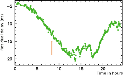
Figure 4: The wide-band a priori group delays at the baseline ceduna/parkes  in experiment v271a on February 05, 2008 after substitution of adjustments to clock function, atmosphere path delay in zenith direction from the narrow-band LSQ solution and source positions from the wide-band LSQ solution at other baselines and group delay ambiguity resolution. The bar in the central side of the plot corresponds to the ambiguity spacing of the wide-band path group delay.

An example of the a priori wide-band group delay with the substituted adjustments to sources positions found from the wide-band group delay solution at other baselines is shown in Fig. 4. After resolving ambiguities for the most of observations, the points that were temporarily suppressed were restored and used in the solution.

5.1.2 Ionosphere path delay contribution

Single band VLBI data are affected by a variable path delay through the ionosphere. We attempted to model this path delay using GPS TEC maps provided by the CODE analysis center for processing Global Navigation Satellite System data (Schaer, 1998). Details of computing the VLBI ionospheric path delay using TEC maps from GPS are given in Petrov et al. (2011). The model usually recovers over 80% of the path delay at baselines longer than several thousand kilometres. However, applying the ionosphere TEC model to processing LCS1 experiment did not improve the solution and even degraded the fit. The same model and software program certainly improved the fit and improved results when applied to processing observations on intercontinental baselines.

In order to investigate the applicability of the reduction for the path delay in the ionosphere based on GPS TEC maps, we processed 29 IVS dual-band geodetic experiments that included the 1089 km long baseline hobart26/parkes. We ran three solutions that included the data only at this baseline. The first reference solution used ionosphere-free linear combinations of X-band and S-band observables. The second solution used X-band only group delays. The third solution used X-band only data and applied the reduction for the path delay in the ionosphere from GPS TEC maps.

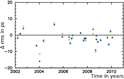
Figure 5: The difference in rms of postfit residuals with respect to the reference dual band X/S solution for two trial solutions: X-band only data (solid discs) and X-band data with ionosphere path delay from GPS TEC map applied (circles).

We discarded two experiments: one had a clock break at hobart26 and another had the rms of postfit residual a factor of 5 greater than usually due to a warm receiver. The rms differences of postfit residuals with respect to the reference dual band X/S solution for two trial solutions are shown in Fig. 5: one with X-band only data and another with X-band data with ionosphere path delays from GPS TEC map applied. Considering the reference solution based on ionosphere-free group delays as the ground truth, we expected that the rms differences between the X-band only solution (denoted with circles in Fig. 5) be positive, and the rms differences of the X-band solution with the ionosphere path delay from GPS TEC maps applied be also positive but less than the rms differences between the X-band only solution. Instead, we see that the rms of postfit residuals of the X-band only solution are less than the rms of dual-band reference solution and applying the ionosphere path delay from GPS TEC maps does not affect the rms significantly.

We then computed the rms of the contribution of the ionosphere path delay from dual-band X/S observations and the rms of the differences between the path delay in the ionosphere from the dual-band X/S observations and the GPS TEC ionosphere maps. They are shown in Fig. 6. We see that in 2002–2004 the ionosphere path delay from GPS TEC maps was coherent with the dual-band ionosphere path delay estimate. In 2005–2010 the ionosphere path delay was small with rms $\sim\!\!30$ ps and the ionosphere path delay from the GPS TEC model was only partially coherent with the ionosphere path delay estimates from dual-band VLBI observations. The baseline length repeatability, defined as the rms of baseline length estimates after subtracting the secular drift due to tectonics, is the minimum when ionosphere-free linear combinations of X/S observables are used: 17.0 mm, grows to 17.4 mm when X-band group delay are used, and it is the maximum, 18.4 mm, when the ionosphere path delay reduction based on GPS TEC model is applied to the X-band observables.

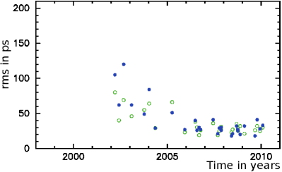
Figure 6: The rms of the ionosphere contribution from dual-band X/S observations (solid disks) and the rms of the differences of the path delay in the ionosphere from the dual-band X/S observations at the baseline hobart26/parkes and the GPS TEC ionosphere maps (circles).

We compared these results with analogous observations in the northern hemisphere. We picked the baseline la–vlba/ov–vlba that has almost exactly the same length as the baseline hobart26/parkes: 1088 km against 1089 km. We processed 88 experiments at this baseline in a similar fashion as we processed the hobart26/parkes baseline. Results are shown in Fig. 7. Applying the ionosphere path delay from GPS has reduced the rms of post-fit residuals at this baseline.

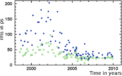
Figure 7: The rms of the ionosphere contribution from dual-band X/S observations (solid disks) and the rms of the differences of the path delay in the ionosphere from the dual-band X/S observations at the 1088 km long baseline la–vlba/ov–vlba and the GPS TEC ionosphere maps (circles).

Our interpretation of this phenomena is that the ionosphere path delay from GPS TEC maps at baselines 1–2 thousands kilometres has the floor around 30 ps. The dominant constituent in the ionospheric path delay at these scales during the solar minimum are short-periodic scintillations that the GPS TEC model with time resolution 2 hours and spatial resolution 500 km does not adequately represent. It is also known (Hernández-Pajares et al., 2009) that the accuracy of the GPS TEC model is worse in the southern hemisphere than in the northern hemisphere due to the disparity in the GPS station distribution.

Applying the GPS TEC map ionosphere path delay reduction effectively added noise in the data. Therefore, we did not apply the ionosphere path delay in our final solution.

5.1.3 Re-weighting observations

According to the Gauss-Markov theorem, the estimate of parameters has the minimum dispersion when observation weights are chosen reciprocal to the variance of errors. The group delays used in the analysis have errors due to the thermal noise in fringe phases and due to mismodeling the propagation delay:

$$\sigma^{2}=\sigma^{2}_{th}+\sigma^{2}_{na}+\sigma^{2}_{io},$$ (4)

where $\sigma_{th}$ is the variance of the thermal noise, $\sigma_{na}$, and $\sigma_{io}$ are the variances of errors of modeling the path delay in the neutral atmosphere and the ionosphere respectively.

A rigorous analysis of the errors of modeling the path delay in the neutral atmosphere is beyond the scope of this paper. Assuming the dominant error source of the a priori model is the high frequency fluctuations of the water vapor at time scales less than 3–5 hours, we sought a regression model for the dependence of $\sigma^{2}_{na}$ on the non-hydrostatic component of the slanted path delay through the atmosphere. We made several trial runs using all observing sessions under geodesy and absolute astrometry programs for 30 years and added in quadrature to the a priori uncertainties of group delay an additive correction:

$$\sigma^{2}_{\rm used}=\sigma_{th}^{2}+\left(a\cdot\frac{\displaystyle\tau_{s}}{\displaystyle\tau_{z}}\right)^{2},$$ (5)

where ${\tau_{s}}$ is the contribution of the non-hydrostatic constituent of the slanted path delay, ${\tau_{z}}$ is the non-hydrostatic path delay in zenith direction computed by a direct integration of equations of wave propagation through the atmosphere using the refractivity computed using the MERRA model, and $a$ is a coefficient. We found that the baseline length repeatability defined as the rms of the deviation of baseline length with respect to the linear time evolution reaches the minimum when $a=0.02$. Therefore, we adopted this value in our analysis of LCS1 experiments. For typical values of ${\tau_{z}}$, the added noise is 8 ps in zenith direction and 16 ps at the elevation of $30^{\circ}$.

We computed the rms of ionosphere contributions from dual band VLBI group delays and from GPS TEC maps. Fig. 8 shows the dependence of the square of the rms from dual-band VLBI versus the square of the rms from GPS. The slope of the regression straight line is $0.992\pm 0.004$. This dependence suggests that although the ionosphere path delay from TEC maps from GPS analysis is too noisy to be applied for reduction of observations at short baselines during the Solar minimum, it correctly predicts the variance of the ionosphere path delay. We assigned the variance of the mismodeled ionosphere path delay to the ionosphere contribution to delay computed from TEC maps: $\sigma_{io}=\tau_{io}$.

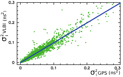
Figure 8: The dependence of the ionosphere path delay $\sigma^{2}_{i}$ from dual-band VLBI versus $\sigma^{2}_{i}$ from TEC maps from GPS analysis. Data in time range 2005.0–2010.6 (Solar minimum) were used.

We also computed, for each experiment and for each baseline, ad hoc variances of observables that after being added in quadrature make the ratio of the weighted sum of squares of post-fit residuals to their mathematical expectation close to unity. This computation technique is presented in Petrov et al. (2011). The ad hoc variance was applied to further inflate the formal uncertainties of the observables that have already been corrected for the inaccuracy of the a priori model of wave propagation through the ionosphere and neutral atmosphere (expression 4). In contrast to $\sigma^{2}_{na}$ and $\sigma^{2}_{io}$, the baseline-dependent ad hoc variance is elevation independent.

5.1.4 Global LSQ solution

We ran a single global LSQ solution using all available dual-band VLBI observations under geodesy and absolute astronomy programs from 1980.04.12 through 2010.08.04, in total 7.56 million observations, and the X-band VLBI data from 4 LCS1 observing sessions. The RCP and LCP data were treated as independent experiments. The following parameters were estimated over the global dataset: coordinates of 4924 sources, including 410 detected target objects in the LCS1 campaign (see Fig. 9); positions and velocities of all stations; coefficients of expansion over the B-spline basis of non-linear motions for 17 stations; coefficients of harmonic site position variations of 48 stations at four frequencies: annual, semi-annual, diurnal, semi-diurnal; and axis offsets for 67 stations. In addition, the following parameters were estimated for each experiment independently: station-dependent clock functions modeled by second order polynomials, baseline-dependent clock offsets, the pole coordinates, UT1-TAI, and daily nutation offset angles. The list of estimated parameters also contained more than 1 million nuisance parameters: coefficients of linear splines that model atmospheric path delay (20 minutes segment) and clock function (60 minutes segment).

The rate of change for the atmospheric path delay and clock function between adjacent segments was constrained to zero with weights reciprocal to $1.1\cdot 10^{-14}$ and $2\cdot 10^{-14}$ respectively in order to stabilize our solution. We apply no-net rotation constraints on position of 212 sources marked as “defining” in the ICRF catalogue (Ma et al., 1998) that requires the positions of these source in the new catalogue to have no rotation with respect to the position in the ICRF catalogue.

The global solution sets the orientation of the array with respect to an ensemble of $\sim\!5000$ extragalactic remote radio sources. The orientation of that ensemble is defined by the series of the Earth orientation parameters evaluated together with source coordinates. Common 111 sources observed in LCS1 as atmosphere and amplitude calibrators provide strong connection between the new catalogue to the old catalogue of compact sources.

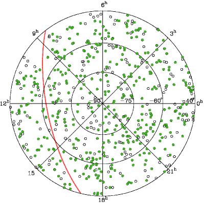
Figure 9: The distribution of sources with milliarcsecond positions at the southern sky. Circles denote sources known by 2008. Filled green discs denote sources from the LCS1 catalogue. The Galactic plane shown by red line.

5.2 Error analysis of the LCS1 catalogue

To assess the systematic errors in our results we exploited the fact that 111 known sources were observed as amplitude and atmospheric calibrators. Positions of these sources were determined from previous dual-band S/X observations with accuracies better than 0.2 mas. We sorted the set of 111 calibrators according to their right ascensions and split them into two subsets of 55 and 56 objects, even and odd. We ran two additional solutions. In the first solution we suppressed 55 calibrators in all experiments but LCS1 and determined their positions solely from the LCS1 experiment. In the second solution we did the same with the second subset. Considering that the positions of calibrators from numerous S/X observations represent the ground truth, we treated the differences as LCS1 errors.

We computed the $\chi^{2}/\mbox{ndf}$ statistics for the differences in right ascensions and declinations $\Delta_{\alpha}$ and $\Delta_{\delta}$ and sought additional variances $v_{\alpha}$ and $v_{\delta}$ that, being added in quadrature to the formal source position uncertainties, $\sigma_{\!\alpha,i}$ and $\sigma_{\!\delta,i}$, make them close to unity:

$$\begin{array}[]{l @{\enskip} c @{\enskip} l}\frac{\chi^{2}_{\alpha}}{\mbox{ndf}}&=&\frac{\displaystyle\sum\Delta\alpha_{i}^{2}\cos^{2}\delta_{i}}{\displaystyle n\,\sum\sqrt{\sigma^{2}_{\alpha,i}\cos^{2}\delta_{i}+v^{2}_{\alpha}}}\vspace{1ex}\\ \frac{\chi^{2}_{\delta}}{\mbox{ndf}}&=&\frac{\displaystyle\sum\Delta\delta_{i}^{2}}{\displaystyle n\,\sum\sqrt{\sigma^{2}_{\delta,i}+v^{2}_{\delta}}}.\end{array}$$ (8)

We found the following additive corrections of the uncertainties in right ascensions scaled by $\cos\delta$ and for declinations respectively: $v_{\alpha}=1.44$ mas and $v_{\delta}$=0.51 mas. We do not have an explanation why the additive correction for scaled right ascensions is 3 times greater than for declinations. After applying the additive corrections, the wrms of source position differences are 1.8 mas for right ascension scaled by $\cos\delta$ and 1.5 mas for declinations.

The final inflated uncertainties of source positions, $\sigma^{2}_{\alpha}(f)$ and $\sigma^{2}_{\delta}(f)$, are

$$\begin{array}[]{l @{\enskip} c @{\enskip} l}\sigma^{2}_{\alpha}(f)=\sigma^{2}_{\alpha}+v^{2}_{\alpha}/\cos^{2}\delta\vspace{1ex}\\ \sigma^{2}_{\delta}(f)=\sigma^{2}_{\delta}+v^{2}_{\delta}.\end{array}$$ (11)

5.3 Data analysis: correlated flux density determination

Each detected source has from 3 to 60 observations, with a median value of 25. Imaging a source with 25 points at the $uv$ plane is a difficult problem, and the dynamic range of such images will be between 1:10 and 1:100, which is far from spectacular. Images produced with the hybrid self-calibration method will be presented in a separate paper. In this study we limited our analysis to mean correlated flux density estimates in three ranges of lengths of the baseline projections onto the plane tangential to the source, without inversion of calibrated visibility data. Information about the correlated flux density is needed for evaluation of the required integration time when an object is used as a phase calibrator.

First, we calibrated raw visibilities $v$ for the a priori system temperature $T_{sys}$ and antenna gain $G(e)$: $A_{corr}=v\cdot T_{sys}(t,e)/G(e)$. The coefficients of antenna gain expansions into polynomials over elevation angle $e$ are presented in Table 4. System temperature was measured at each station, each scan.

Table 4: The coefficients of antenna gain polynomials over elevation angle expressed in radians. Gain = DPFU $\displaystyle\sum_{k=0}^{k=5}a_{k}E^{k}$. The DFPU is shown in the second columns. Columns 3–8 hold coefficients of degree 0 through 5.

Station	DFPU K/Jy	The coefficients of polynomial for gain as a function of the elevation angle in degrees
		0 aa	1 aaaa	aa 2	aa 3	aa 4	aa 5
atca-104	$0.100$	$1.0$	$0.0$	$\hphantom{-}0.0$	$\hphantom{-}0.0$	$\hphantom{-}0.0$	$\hphantom{-}0.0$
ceduna	$1.000$	$0.9045$	$4.032\cdot 10^{-3}$	$-4.280\cdot 10^{-5}$	$\hphantom{-}0.0$	$\hphantom{-}0.0$	$\hphantom{-}0.0$
dss45	$0.240$	$0.9700$	$2.927\cdot 10^{-3}$	$-1.070\cdot 10^{-4}$	$\hphantom{-}1.761\cdot 10^{-6}$	$-1.112\cdot 10^{-8}$	$\hphantom{-}0.0$
hobart26	$0.058$	$0.6997$	$4.445\cdot 10^{-2}$	$-2.331\cdot 10^{-3}$	$\hphantom{-}5.335\cdot 10^{-5}$	$-5.412\cdot 10^{-7}$	$\hphantom{-}1.926\cdot 10^{-9}$
mopra	$0.095$	$1.0$	$0.0$	$\hphantom{-}0.0$	$\hphantom{-}0.0$	$\hphantom{-}0.0$	$\hphantom{-}0.0$
parkes	$0.480$	$0.7900$	$3.368\cdot 10^{-3}$	$\hphantom{-}8.507\cdot 10^{-5}$	$-1.398\cdot 10^{-6}$	$\hphantom{-}0.0$	$\hphantom{-}0.0$

At the second step, we adjusted antenna gains using publicly available brightness distributions of calibrator sources made with observations under other programs. We compiled The Database of Brightness Distributions, Correlated Flux Densities and Images of Compact Radio Sources Produced with VLBI from authors who agreed to make their imaging results publicly available. Among 111 sources observed as calibrators, images of 14–27 objects at each experiment were available. These are images in the form of CLEAN components mainly from Ojha et al. (2004, 2005). CLEAN components of source brightness distributions from analysis of the TANAMI program (Ojha et al., 2010) that observed with the LBA concurrently with the LCS1 were not available, but the parameters of one-component Gaussian models that fit the core regions were published. For those sources for which both a set of CLEAN components and the parameter of the Gaussian one-component model were available, we used CLEAN components.

We predicted the correlated flux density $F_{corr}$ for each observation of an amplitude calibrator with known brightness distribution, as

$$\begin{array}[]{lcl}F_{corr}&=&\left|\displaystyle\sum_{i}c_{i}e^{\frac{2\pi\,f}{c}\,(u\,x+v\,y)}\right|\\ F_{corr}&=&S\,e^{\frac{\pi^{2}}{4\ln 2}\,(a^{2}\,(u\cos\theta+v\sin\theta)^{2}+b^{2}\,(-u\sin\theta+v\cos\theta)^{2})},\end{array}$$ (14)

where $c_{i}$ is the correlated flux density of the $i$th CLEAN component with coordinates $x$ and $y$ with respect to the center of the image; $u$ and $v$ are the projections of the baseline vectors on the tangential plane of the source; and $a$ and $b$ are the FWHM of the Gaussian that approximates the core, and $\theta$ is the position angle of the semi-major axis of the Gaussian model.

Then we built a system of least square equations for all observations of calibrators with known images used in astrometric solutions:

$$F_{corr}=\sqrt{g_{i}\,g_{j}}A_{corr}$$ (15)

and after taking logarithms from left and right hand sides solved for corrections to gains $g$ for all stations. Finally, we applied corrections to gain for observations of all other sources.

The correlated flux density is a constant during observing session only for unresolved sources. For resolved sources the correlated flux density depends on the projection of the baseline vector on the source plane and on its orientation. We binned the correlated flux densities in three ranges of the baseline vector projection lengths, 0–6 M$\lambda$, 6–25 M$\lambda$, 25–50 M$\lambda$, and found the median value within each bin. These bins correspond to scales of the detected emission at $>30$ mas, 7–30 mas, and $<7$ mas respectively.

The uncertainties of our estimates of the correlated density depend on the thermal noise described as $\sigma_{th}=F_{corr}/{\mbox{\rm SNR}}$ and errors of gain calibration. The variance of the thermal noise was in the range of 1 to 6 mJy depending on the sensitivity of a baseline, with the median value of 3 mJy. The LSQ solution for gains provided the variance of the logarithm of gains. Assuming the calibration errors to be multiplicative in the form $g\,(1+\epsilon)$, where $g$ is gain and $\epsilon$ is the Gaussian random variable, we can evaluate the contribution of gain errors in the multiplicative uncertainty of $F_{corr}(1+\mu)$, where $\mu$ the Gaussian random variable. Its variance is evaluated as

$$\begin{array}[]{l}\sigma(\mu)=\\ \exp\left(\frac{1}{2}\sqrt{\mathop{\rm Cov}\nolimits(s_{1},s_{1})+\mathop{\rm Cov}\nolimits(s_{2},s_{2})+2\mathop{\rm Cov}\nolimits(s_{1},s_{2})}\right),\end{array}$$ (18)

where $\mathop{\rm Cov}\nolimits(s_{i},s_{j})$ is the covariance of the logarithm of gain between the $i$-th and $j$-th station. Multiplicative gain uncertainties are in the range 0.08–0.1 for dss45 and 0.02–0.05 for other stations. The gain uncertainties for dss45 are higher, because it observed 3–5 times less than other stations. The total variance is a sum in quadrature of $\sigma_{c}$ and $\sigma_{th}$. We should note that our estimate of systematic errors does not account for possible errors in gain curve determination. A systematic error in the gain curve would directly affect our estimate of the correlated flux density. It will also affect the maps of calibrators sources that we took from literature, and thus indirectly affect our estimates of gain corrections. We do not have information about uncertainties of gain curves of LBA antennas.

Table 5: The first 12 rows of the catalogue of source correlated flux density estimates for both 410 target sources and 111 calibrator sources in each experiment. Some sources were observed on more than one experiment. The table columns are explained in the text. The full table is available in the electronic attachment.

J2000-name	B1950-name	Date	Sts	# Obs	Corr. flux density (Jy)			Flux density uncertainties (Jy)			Exp
J0004$-$4736	0002$-$478	2008.11.28		12	0.352	0.268	0.267	0.015	0.019	0.013	v271b
J0011$-$8443	0009$-$850	2008.02.05		30	0.161	0.165	0.180	0.005	0.005	0.006	v254b
J0012$-$3954	0010$-$401	2008.02.05		16	0.761	0.769	0.715	0.016	0.012	0.014	v254b
J0012$-$3954	0010$-$401	2009.07.04	Cal	10	0.815	0.654	0.640	0.026	0.023	0.028	v271c
J0028$-$7045	0026$-$710	2008.11.28		40	0.092	0.086	0.081	0.005	0.006	0.005	v271b
J0030$-$4224	0027$-$426	2009.07.04		30	0.312	0.290	0.256	0.011	0.010	0.011	v271c
J0033$-$4236	0031$-$428	2009.07.04		30	0.132	0.135	0.143	0.005	0.005	0.008	v271c
J0034$-$4116	0031$-$415	2009.07.04		18	0.053	0.045	0.039	0.003	0.002	0.004	v271c
J0040$-$4253	0038$-$431	2009.07.04		28	0.068	0.058	0.067	0.003	0.002	0.007	v271c
J0042$-$4030	0039$-$407	2009.07.04		26	0.255	0.253	0.276	0.010	0.011	0.013	v271c
J0042$-$4333	0040$-$438	2009.07.04		30	0.165	0.113	0.126	0.005	0.005	0.008	v271c
J0044$-$8422	0044$-$846	2008.02.05		26	0.278	0.255	0.234	0.007	0.006	0.007	v254b

Table 5 displays 12 out of 633 rows of the catalogue of correlated flux density estimates. The full table is available in the electronic attachment. Column 1 and 2 contain the J2000 and B1950 IAU names of a source; column 3 contains the observation date of the experiment; the 4th column contains the status of the source: Cal if it was used as amplitude calibrator; the 5th columns contains the number of RCP observations used in processing. Columns 6, 7, and 8 contain median values of correlated flux densities determined in that experiment at baseline projection lengths 0–6 $M\lambda$, 6–25 $M\lambda$, and 25–50 $M\lambda$ respectively. Columns 9, 10, and 11 contain the arithmetic mean of correlated flux density uncertainties that accounts for both thermal noise and uncertainties in calibration. If no data were collected to that range of baseline projection lengths, $-1.0$ is used as a substitute. Column 12 contains the experiment name.

Fig. 10 shows the probability density histogram of correlated flux densities in LCS1 experiments.

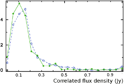
Figure 10: The probability density histogram of correlated flux densities in LCS1 experiments. The dotted line with dicks denotes correlated flux densities at baseline projection lengths 0–6 M$\lambda$, the solid line with discs denotes the correlated flux density at projection lengths 25–50 M$\lambda$,

6 The LCS1 catalogue

Table 6 displays 12 out of 410 rows of the LCS1 catalogue of source positions. The full table is available in the electronic attachment. Column 1 and 2 contain the J2000 and B1950 IAU names of a source; column 3, 4, and 5 contain hours, minutes and seconds of the right ascension; columns 6, 7, 8 contain degrees, minutes and arcseconds of declination. Columns 9 and 10 contain inflated position uncertainties in right ascension (without multiplier $\cos\delta$) and declination in milliarcseconds. Column 11 lists the correlation coefficient between right ascension and declination, and column 12 contains the total number of observations used in position data analysis, including RCP and LCP data. Columns 13, 14, and 15 contain the median estimates of the correlated flux density in Jansky over all experiment of the source in three ranges of baseline projection lengths: 0–6 $M\lambda$, 6–25 $M\lambda$, and 25–50 $M\lambda$. Columns 16, 17, and 18 contain estimates of the correlated flux density uncertainties in Jansky.

Table 6: The first 12 rows of the LCS1 catalogue of source positions of 410 target sources. The table columns are explained in the text. The full table is available in the electronic attachment.

J2000-name	B1950-name	Right ascension			Declination			$\sigma(\alpha)$	$\sigma(\delta)$	Corr	#Obs	Correl. Flux			Correl. Flux uncer.
								(9)	(10)	(11)	(12)	(13)	(14)	(15)	(16)	(17)	(18)
		h	m	s	∘	′	′′	mas	mas			Jy	Jy	Jy	Jy	Jy	Jy
J0011$-$8443	0009$-$850	00	11	45.90267	$-$84	43	20.0096	46.1	3.1	-0.228	30	0.162	0.165	0.180	0.005	0.005	0.006
J0028$-$7045	0026$-$710	00	28	41.56281	$-$70	45	15.9267	7.1	1.7	0.006	40	0.092	0.086	0.081	0.005	0.006	0.005
J0030$-$4224	0027$-$426	00	30	17.49264	$-$42	24	46.4827	2.0	1.4	-0.036	37	0.312	0.290	0.256	0.011	0.010	0.011
J0033$-$4236	0031$-$428	00	33	47.94145	$-$42	36	14.0676	3.7	2.2	-0.012	37	0.132	0.135	0.143	0.005	0.005	0.008
J0034$-$4116	0031$-$415	00	34	04.40893	$-$41	16	19.4729	7.1	3.6	0.089	25	0.053	0.045	0.039	0.003	0.002	0.004
J0040$-$4253	0038$-$431	00	40	32.51473	$-$42	53	11.3916	4.5	2.8	0.057	35	0.068	0.058	0.067	0.003	0.002	0.007
J0042$-$4030	0039$-$407	00	42	01.22481	$-$40	30	39.7419	3.4	2.0	0.013	33	0.255	0.253	0.276	0.010	0.011	0.013
J0042$-$4333	0040$-$438	00	42	24.86725	$-$43	33	39.8164	3.9	2.3	0.002	37	0.165	0.113	0.126	0.005	0.005	0.008
J0044$-$8422	0044$-$846	00	44	26.68719	$-$84	22	39.9895	44.0	2.9	-0.237	30	0.278	0.255	0.234	0.007	0.006	0.007
J0047$-$7530	0046$-$757	00	47	40.81228	$-$75	30	11.3640	6.4	1.4	-0.631	41	0.139	0.118	0.078	0.006	0.008	0.006
J0049$-$4457	0046$-$452	00	49	16.62412	$-$44	57	11.1658	3.7	2.1	-0.005	37	0.244	0.215	0.207	0.009	0.006	0.011
J0054$-$7534	0052$-$758	00	54	05.81337	$-$75	34	03.6325	6.3	1.4	-0.803	44	0.094	0.087	0.080	0.004	0.007	0.006

Of 421 sources observed, 410 were detected in three or more scans. In four LCS1 observing sessions, 17,731 observations out of 19,494 were used in the LSQ solution together with 7.56 million other VLBI observations. The semi-major error ellipse of inflated position uncertainties varies in the range 1.4 to 16.8 mas with the median value of 2.6 mas. The distribution of sources on the sky is presented in Fig. 9. The histogram of position errors is shown in Fig. 11.

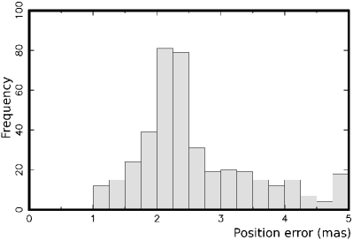
Figure 11: The histogram of the semi-major axes of inflated position error ellipses among 410 sources in the LCS1 catalogue.

7 Summary

The absolute astrometry LBA observations turned out highly successful. The overall detection rate was 97% — the highest rate ever achieved in a VLBI survey. If we exclude extended sources, non-AT20G sources and the six planetary nebulae included in the candidate list due to an oversight, the detection rate is 99.8%! We attribute this high detection rate to two factors. Firstly, the AT20G catalogue is highly reliable and is biased towards very compact objects. Selecting candidates based on the simultaneous AT20G spectral index proves to be a good methodology. Secondly, the LBA has very high sensitivity. The baseline detection limit over 2 minute of integration time varied from 7 mJy to 30 mJy, with 7–12 mJy at baselines with parkes.

We have successfully resolved group delay ambiguities with spacing 3.9 ns for all observations. This became possible using the innovative algorithm exploiting relatively low level of instrumental group delay errors.

We have determined positions of 410 target sources never before observed using VLBI, with a median uncertainty of 2.6 mas. Error analysis showed a moderate contribution of the mismodeled ionosphere path delay to the overall error budget. Both random and systematic errors are accounted for in the uncertainties ascribed to source positions exploiting the overlap of 111 additional sources observed in LCS1 experiments with their positions known from prior observations. The positional accuracy of the LCS1 catalogue is a factor of 350 greater than the positional accuracy of the AT20G catalogue, corresponding to the ratio of the maximum baseline lengths of the LBA and the ATCA. The new catalogue has increased the number of sources with declinations $<-40\degr$ from 158 to 568, i.e. by a factor of 3.5.

We determined correlated flux densities for 410 target and 111 calibrator sources, and presented their median values in three ranges of baseline projection lengths. The correlated flux density of the target sources varied from 0.02 to 2.5 Jy, and was in the range 80–300 mJy for 70% of the sources. The uncertainties of the correlated flux densities are estimated to be typically 5–8%.

This observing program is continuing. By November 2010, four additional twenty four hour experiments had been observed with several more observing sessions planned.

8 Acknowledgments

The authors would like to thank Anastasios Tzioumis for comments which helped to improve the manusrcipt. The authors made use of the database CATS of the Special Astrophysical Observatory. We used in our work the dataset MAI6NPANA provided by the NASA/Global Modeling and Assimilation Office (GMAO) in the framework of the MERRA atmospheric reanalysis project. The Long Baseline Array is part of the Australia Telescope National Facility which is funded by the Commonwealth of Australia for operation as a National Facility managed by CSIRO.

References

- Beasley et al. (2002) Beasley A. J., Gordon D., Peck A. B., Petrov L., MacMillan D. S., Fomalont E. B., Ma C., 2002, ApJS, 141, 13
- Cohen & Shaffer (1971) Cohen M. H. & Shaffer D. B., 1971, AJ, 76, 91.
- Deller et al. (2009) Deller A. T., Tingay S. J., Bailes M., Reynolds J. E., 2009, ApJ, 701, 1234
- Eichhorn et al. (2002) Eichhorn, G., Accomazzi, A., Grant, C. S., Kurtz, M. J., Murray, S. S., 2002, Ap&SS, 282, 299
- Farrell (1972) Farrell W. E., 1972, Rev. Geophys. and Spac. Phys., 10(3), 751
- Fey et al. (2004) Fey A. et al., 2004, AJ, 127, 1791
- Fey et al. (2006) Fey A. et al., 2006, AJ, 132, 1944
- Fomalont et al. (2003) Fomalont E., Petrov L., McMillan D. S., Gordon D., Ma C. 2003, AJ, 126, 2562
- Hernández-Pajares et al. (2009) Hernández-Pajares M. et al., 2009, Jour. Geodesy, 83, 263
- Kalnay et al. (1996) Kalnay E. M. et al., 1996, Bull. Amer. Meteorol. Soc., 77, 437–471
- Kopeikin & Schäfer (1999) Kopeikin S. M. & Schäfer G., 1999, Phys Rev D, 60(12), 124002
- Kovalev et al. (2007) Kovalev Y. Y., Petrov L., Fomalont E., Gordon D., 2007, AJ, 133, 1236
- Lanyi et al. (2010) Lanyi G. E. et al., 2010, AJ, 139, 1695
- Ma et al. (1998) Ma C. et al., 1998, AJ, 116, 516
- Massardi et al. (2010) Massardi M. et al., 2010, MNRAS, 412, 318
- Mathews (2001) Mathews P.M., 2001, J Geod Soc Japan, 47(1), 231–236
- Matsumoto, Takanezawa & Ooe (2000) Matsumoto K., Takanezawa T., Ooe M., 2000, J Oceanography, 56, 567–581
- Matveenko, Kardashev & Sholomitskii (1965) Matveenko L. I., Kardashev N. S., Sholomitskii G. B., 1965, Izvestia VUZov. Radiofizika, 8, 651 (English transl. Soviet Radiophys., 8, 461)
- Murphy et al. (2010) Murphy T. et al., 2010, MNRAS, 420, 2403
- Ojha et al. (2004) Ojha R. et al., 2004, AJ, 127(6), 3609
- Ojha et al. (2005) Ojha R. et al., 2005, AJ, 130, 2529
- Ojha et al. (2010) Ojha R. et al., 2010, A&A, 519, A45
- Petrov (2007) Petrov L., 2007, A&A, 467(1), 359
- Petrov & Ma (2003) Petrov L., Ma C., 2003, J Geophys Res, 108(B4), 2190
- Petrov & Boy (2004) Petrov L., Boy J.-P., 2004, J Geophys Res, 109, B03405
- Petrov et al. (2005) Petrov L., Kovalev Y. Y., Fomalont E., Gordon D., 2005, AJ, 129, 1163
- Petrov et al. (2006) Petrov L., Kovalev Y. Y., Fomalont E., Gordon D., 2006, AJ, 131, 1872
- Petrov et al. (2007a) Petrov L., Kovalev Y. Y., Fomalont E., Gordon D., 2007a, AJ, 136, 580
- Petrov et al. (2007b) Petrov L., Hirota T., Honma M., Shibata S. M., Jike T., Kobayashi H., 2007b, AJ, 133, 2487
- Petrov et al. (2009a) Petrov L., C. Phillips, A. Bertarini, A. Deller, S. Pogrebenko, A. Mujunen, 2009a, PASA, 26(1), 75
- Petrov et al. (2009b) Petrov L., Gordon D., Gipson J., MacMillan D., Ma C., Fomalont E., Walker R. C., Carabajal C., 2009b, Jour. Geodesy, 83(9), 859
- Petrov et al. (2011) Petrov L., Kovalev Y. Y., Fomalont E., Gordon D., 2011, AJ, 142:35(23pp)
- Phillips et al. (2009) Phillips C., Tzioumis T., Tingay S., Stevens J., Lovell J., Amy S., West C., Dodson R., 2009, in Proc. Science and Technology of Long Baseline Real-Time Interferometry The 8th International e-VLBI Workshop, EXPReS09, 99 (http://pos.sissa.it/cgi-bin/reader/ conf.cgi?confid=82)
- Ray (1999) Ray R. D., 1999, NASA/TM-1999-209478, Greenbelt, MD USA
- Rodell et al. (2004) Rodell M., et al., 2004, Bull. Amer. Meteor. Soc., 85(3), 381
- Schubert et al. (2008) Schubert S. et al., In Proc. of Third WCRP International Conference on Reanalysis, Tokyo, 2008, V1–104 (http://wcrp.ipsl.jussieu.fr/Workshops/Reanalysis2008/ Documents/V1-104_ea.pdf)
- Sovers, Fanselow & Jacobs C.S (1998) Sovers O. J., Fanselow J. L., Jacobs C. S., 1998, Rev Modern Phys, 70(4), 1393–1454
- Schaer (1998) Schaer S., 1998, PhD thesis, Univer. Bern (ftp://ftp.unibe.ch/aiub/papers/ionodiss.ps.gz)
- Takahashi et al. (2000) Takahashi F., Kondo R., Takahashi Y., Koyama Y., 2000, Very long baseline interferometer, Ohmsha, Ltd, Tokyo
- Verkhodanov et al. (1997) Verkhodanov O. V., Trushkin S. A., Andernach H., Chernenkov V. N., 1997, in G. Hunt, H. E. Payne, eds., ASP Conf. Ser. 125, Astronomical Data Analysis Software and Systems VI, p. 322
- Whitney et al. (2004) Whitney A. R. et al., 2004, Radio Sci, 39, RS1007
- Wrobel (2009) Wrobel J., 2009, NRAO eNews, 2(11), 6(http://www.nrao.edu/news/newsletters/enews/ enews_2_11/enews_2_11.pdf)