Poisson–Dirichlet branching random walks

Abstract

We determine, to within $O(1)$, the expected minimal position at level $n$ in certain branching random walks. The walks under consideration have displacement vector $(v_{1},v_{2},\ldots)$, where each $v_{j}$ is the sum of $j$ independent $\operatorname{Exponential}(1)$ random variables and the different $v_{i}$ need not be independent. In particular, our analysis applies to the Poisson–Dirichlet branching random walk and to the Poisson-weighted infinite tree. As a corollary, we also determine the expected height of a random recursive tree to within $O(1)$.

and t1Supported by an NSERC Discovery Grant. t2Supported by NSF Grant DMS-09-01339. The research was conducted in part while the K. Ford was visiting the Institute for Advanced Study, supported by grants from the Ellentuck Fund and The Friends of the Institute For Advanced Study.

1 Introduction

A branching random walk starts from an initial particle, the root, with position $0$. The root produces some number of children, who are randomly displaced from their parent according to some displacement law. Each child in turn produces some number of children, who are displaced from the position of their parent according to the same law; and so on. In general, the displacements of siblings relative to their parent may be dependent, but for distinct particles $v$ and $w$, the displacements of the children of $v$ and of the children of $w$ must be independent. When the displacements are nonnegative, this is often called an age-dependent branching process, and the displacements are thought of as “times to birth.”

There is a natural tree associated with a branching random walk, where the vertices correspond to particles, and an edge from parent to child is weighted with the child’s displacement from its parent. More precisely, let $T$ be the Ulam–Harris tree, which has vertex set $V=\bigcup_{n=0}^{\infty}\mathbb{N}^{n}$ (we think of elements of $\mathbb{N}^{n}$ as concatenations of $n$ integers, and take $\mathbb{N}^{0}=\{\varnothing\}$), is rooted at $\varnothing$, and has an edge from $v$ to $vi$ for each $v\in V$ and each $i\in\mathbb{N}$. We call $\mathbb{N}^{n}$ the $n$th generation of $T$, and for $v=v_{1},\ldots,v_{n}\in\mathbb{N}^{n}$, we say that $v$ has parent $p(v)=v_{1},\ldots,v_{n-1}$ and children $vi$, $i\in\mathbb{N}$. (We will usually write $T_{n}$ in place of $\mathbb{N}^{n}$ for readability.)

Now suppose $\mathbf{X}=(X_{i}\dvtx i\in\mathbb{N})$ is a random vector, where each $X_{i}\in\mathbb{R}\cup\{+\infty\}$. We do not require that the entries of $\mathbf{X}$ are independent of one another—this will be important below. Then we form a branching random walk by marking each vertex $v\in V$ with an independent copy $\mathbf{X}^{v}=(X^{v}_{i}\dvtx i\in\mathbb{N})$ of $\mathbf{X}$. Write $\mathcal{T}$ for the pair $(T,\{\mathbf{X}^{v}\dvtx v\in V\})$; then $\mathcal{T}$ is our branching random walk. We call $\mathbf{X}$ the displacement vector of $\mathcal{T}$. For each $v\in V$ and $i\in\mathbb{N}$, we regard $X^{v}_{i}$ as the displacement from $v$ to $vi$, and let $S(v)=S(v,\mathcal{T})$ be the sum of the displacements on the path from the root to $v$ [formally, if $v=v_{1},\ldots,v_{n}$, then $S(v)=\sum_{i=1}^{n}X^{p(v_{1},\ldots,v_{i})}_{v_{i}}$, and this sum is taken to be $+\infty$ if any of its elements are $+\infty$]. We say $\mathcal{T}$ has finite branching if almost surely all but finitely many coordinates of $\mathbf{X}$ are equal to $+\infty$.

For $n\in\mathbb{N}$, let $M_{n}=\inf(S(v)\dvtx v\in\mathbb{N}^{n})$. In all situations we consider in this paper, this infimum is attained, so $M_{n}$ is the minimal displacement of any individual in the $n$th generation. The minimal displacement is one of the most well-studied parameters associated with branching random walks. It has been known since the 1970s hammersly74postulates , kingman75first , biggins76first that under quite general conditions, $M_{n}$ grows asymptotically linearly with lower-order corrections. Recently there have been substantial developments in understanding the finer behavior of $M_{n}$ on two fronts: first, convergence results for the lower order corrections addario07brw , aidekon10weak , hu2009 ; and second, the concentration of $M_{n}$ about its mean (or median) addario07brw , bramson06tightness , chauvin05random . We refer to these as the global behavior and the local behavior of $M_{n}$, respectively. Under suitable conditions, $M_{n}$ generally seems to exhibit the following behavior: for some constants $\alpha\in\mathbb{R}$ and $\beta>0$, $\operatorname{median}(M_{n})=\alpha n+\beta\log n+O(1)$, and, furthermore, $M_{n}/n\to\alpha$ almost surely and $(M_{n}-\alpha n)/\log n\to\beta$ in probability (but not almost surely hu2009 ). Also, under sufficiently strong moment conditions for the displacements, $\mathbb{E}\{\exp(\gamma|M_{n}-\mathbb{E}{M_{n}}|)\}<\infty$ for some $\gamma>0$ and all $n$. (In fact, in some cases the upper tail of $M_{n}-\mathbb{E}{M_{n}}$ is even known to decay doubly-exponentially quickly bachman_brw , ford09pratt .)

To date, however, all the results of the kind described in the preceding paragraph that we are aware of require that the branching random walk has finite branching. In this paper we study the global behavior of $M_{n}$ for a class of branching random walks which do not have finite branching. The class we consider is rather restricted but nonetheless contains at least two interesting special cases, one related to the factorization of random integers, and one related to the analysis of algorithms. Say that $\mathbf{X}$ has exponential steps if for all $i$, $X_{i}$ is distributed as the sum of $i$ independent $\operatorname{Exponential}(1)$ random variables. The main result of this paper is the following theorem. For short, we denote

$$\widetilde{M}_{n}=\operatorname{median}(M_{n}):=\sup\bigl{\{}x\dvtx\mathbb{P}\{M_{n}<x\}<1/2\bigr{\}}.$$

Theorem 1.1

If $\mathbf{X}$ has exponential steps, then

$$\widetilde{M}_{n}=\frac{n}{e}+\frac{3}{2e}\log n+O(1).$$

Remark 1.

The $O(1)$ term is uniform over $n$ and over all BRW for which $\mathbf{X}$ has exponential steps.

Remark 2.

Independently of the current work, Élie Aïdékon aidekonpaper has recently proved, for a quite general family of random walks (including those considered in this paper), that $M_{n}-\widetilde{M}_{n}$ converges in distribution to a random variable $M^{*}$, and describes the distribution of $M^{*}$ in terms of a functional of the limit of the derivative martingale associated to the branching random walk.

Using methods from ford09pratt , we can deduce from Theorem 1.1 uniform exponential tails for $M_{n}$. In the next theorem and at other points throughout the paper, we will use the Vinogradov notation $f\ll g$ which means $f=O(g)$, with subscripts indicating dependence on any parameter, for example, $f\ll_{k}g$ means the constant implied by the $\ll$ symbol may depend on $k$ but not on any other variable.

Theorem 1.2

If $\mathbf{X}$ has exponential steps, then for any $c_{1}<e$, we have

$$\mathbb{P}\{M_{n}\leq\widetilde{M}_{n}-x\}\ll_{c_{1}}e^{-c_{1}x}\qquad(n\geq 1,x\geq 0)$$

and for any $c_{2}<1$,

$$\mathbb{P}\{M_{n}\geq\widetilde{M}_{n}+x\}\ll_{c_{2}}e^{-c_{2}x}\qquad(n\geq 1,x\geq 0).$$

Again, the above estimates are uniform over all BRW under consideration. Also, Theorem 1.2 implies that $\widetilde{M}_{n}=\mathbb{E}{M_{n}}+O(1)$, and so both Theorems 1.1 and 1.2 hold with $\widetilde{M}_{n}$ replaced by $\mathbb{E}{M_{n}}$.

The simplest example of a displacement vector with exponential steps is obtained by taking $\mathbf{X}=(E_{1},E_{1}+E_{2},\ldots)$, where $\{E_{i}\}_{i\in\mathbb{N}}$ are i.i.d.$\operatorname{Exponential}(1)$ random variables. In this case $\mathcal{T}$ is called the Poisson-weighted infinite tree aldous2004omp and has been used very effectively in probabilistic combinatorial optimization. It also arises in the analysis of an important tree-based data structure in the following way. Order the elements of $\mathcal{T}$ in increasing order of displacement as $\{w_{i}\}_{i\in\mathbb{N}}$, so, in particular, we have $w_{1}=\varnothing,w_{2}=1\in\mathbb{N}^{1}$, and either $w_{3}=2\in\mathbb{N}^{1}$ or $w_{3}=11\in\mathbb{N}^{2}$. Now for each $m$ let $Z_{m}$ be the subtree of $\mathcal{T}$ induced by $w_{1},\ldots,w_{m}$. By the memoryless property of the exponential, it follows that the parent of $w_{m+1}$ is a uniformly random element of $Z_{m}$—in other words, $Z_{m}$ is a random recursive tree for all $m$. This connection is well known pittel94recursive .

$Z_{m}$ is also the subtree of $\mathcal{T}$ induced by the set of nodes of displacement at most $S(w_{m})$. [Also, it is straightforwardly shown by induction and the memoryless property of the exponential that the families $(Z_{m})_{m\in\mathbb{N}}$ and $(S(w_{m}))_{m\in\mathbb{N}}$ are independent, but we will not need this.] Let $H_{m}$ be the height of $Z_{m}$—the largest generation containing a node of $Z_{m}$. In other words, $H_{m}=\max\{n\dvtx M_{n}\leq S(w_{m})\}$, which is the representation that will be useful below. Devroye devroye87branching showed that $H_{m}/\log m\to e$ almost surely and in expectation, and Pittel pittel94recursive provided a different proof of the almost sure convergence. As a straightforward consequence of Theorems 1.1 and 1.2, we obtain the following more precise information.

Corollary 1.3

The height $H_{m}$ of a random recursive tree on $m$ nodes satisfies $\mathbb{E}{H_{m}}=e\log m-\frac{3}{2}\log\log m+O(1)$. Furthermore, for all $c^{\prime}<\frac{1}{2e}$, all $m\geq 1$, $k\geq 1$,

$$\mathbb{P}\{|H_{m}-\mathbb{E}{H_{m}}|\geq k\}\ll_{c^{\prime}}e^{-c^{\prime}k}.$$

Since the proof of this corollary is very short, we include it in the Introduc- tion. In the proof we write $\operatorname{har}(s)=\sum_{i=1}^{s}1/i$. Proof of Corollary 1.3 The random variable $S(w_{m})$ is distributed as the sum, $F_{1}+\cdots+F_{m-1}$, of independent random variables with $F_{i}$ having $\operatorname{Exponential}(i)$ distribution for $i=1,\ldots,m-1$. Equivalently, $S(w_{m})$ is distributed as the maximum of $m-1$ i.i.d. $\operatorname{Exponential}(1)$ random variables. Thus, $\mathbb{E}{S(w_{m})}=\operatorname{har}(m-1)$ and for all $x>0$,

$$\qquad\mathbb{P}\{S(w_{m})\geq\operatorname{har}(m-1)+x\} \leq (m-1)e^{-(\operatorname{har}(m-1)+x)}\leq e^{-x},$$ (1)

$$\mathbb{P}\{S(w_{m})\leq\operatorname{har}(m-1)-x\} = \bigl{(}1-e^{-(\operatorname{har}(m-1)-x)}\bigr{)}^{m-1}\leq e^{-e^{x-1}}.$$ (2)

Now write

$$d(m)=\max\{n\dvtx\widetilde{M}_{n}\leq\operatorname{har}(m-1)\}=e\log m-\tfrac{3}{2}\log\log m+O(1)$$

and note that $\widetilde{M}_{d(m)}=\operatorname{har}(m-1)+O(1)$ by Theorem 1.1. It follows that for $k\geq 1$, if $H_{m}\geq d(m)+k$, then either

$$M_{d(m)+k}\leq\operatorname{har}(m-1)+\frac{k}{2e}\leq\widetilde{M}_{d(m)+k}-\frac{k}{2e}+O(1),$$

or

$$S(w_{m})\geq\operatorname{har}(m-1)+\frac{k}{2e}.$$

By Theorem 1.2 and (1), it follows that $\mathbb{P}\{H_{m}\geq d(m)+k\}\ll_{c_{1}}e^{-c_{1}k/(2e)}$ for each $c_{1}<e$. A similar argument using Theorem 1.2 and (2) shows the bound $\mathbb{P}\{H_{m}\leq d(m)-k\}\ll_{c_{2}}e^{-c_{2}k/(2e)}$ for each $c_{2}<1$.

Another important example of a displacement vector with exponential steps arises from a discrete time random fragmentation process. Let $U_{1},U_{2},\ldots$ be independent uniform $[0,1]$ random variables. Set $G_{1}=U_{1}$ and for $i>1$ set $G_{i}=(1-U_{1})\cdot\,\cdots\,\cdot(1-U_{i-1})U_{i}$. The distribution of the sequence

$${\mathbf{G}}=(G_{1},G_{2},\ldots)$$

was first studied, in greater generality, in halmos_alms . (One motivation for Halmos’ paper was a problem about loss of energy of neutrons after many collisions; after each collision the neutron loses a random fraction of its current energy.) ${\mathbf{G}}$ is also a special case of the Griffiths–Engen–McCloskey $\operatorname{GEM}$ distribution. Further, $(G_{\sigma(1)},G_{\sigma(2)},\ldots)$ has the Poisson–Dirichlet (or $\operatorname{PD}$) distribution, where $\sigma\dvtx\mathbb{N}\to\mathbb{N}$ is the permutation that arranges the terms of $(G_{1},G_{2},\ldots)$ in decreasing order. (We remark that both the $\operatorname{GEM}$ and the $\operatorname{PD}$ distributions as defined above are in fact special cases from a more general two-parameter family of distributions pitman2002csp —in the standard notation, we are considering the $\operatorname{GEM}(0,1)$ and $\operatorname{PD}(0,1)$ distributions.) The PD distribution arises in a number of natural decomposition situations, such as factorization of large random integers Bil72 , donnelly1993asymptotic and cycle lengths of random permutations pitman2002csp .

Letting $X_{k}=-\log G_{k}$ for each $k$ yields a vector $(X_{1},X_{2},\ldots)$ with exponential steps. We refer to the resulting branching random walk as a Poisson–Dirichlet branching random walk. This example has more complicated dependence between the $X_{i}$ than the first example. Since $\sum_{i=1}^{\infty}G_{i}=1$ almost surely, there is another way to think of the branching random walk. Imagine that an object of mass $m$ is placed at the root $\varnothing$. The root divides this mass into pieces according to the vector ${\mathbf{G}}^{\varnothing}$ and sends the pieces to its children, sending a mass $mG_{k}^{\varnothing}$ to its $k$th child. This rule is repeated recursively, so each node $v$ sends proportion $G_{k}^{v}$ of the mass it receives to its $k$th child $vk$. This structure is variously called a multiplicative cascade or, more commonly at the moment, a fragmentation process bertoin2006rfa . The special case of Theorem 1.1 when $\mathcal{T}$ is a Poisson–Dirichlet branching random walk is used in ford09pratt to analyze a tree model related to primality testing, proving heuristic evidence for the behavior of the distribution of tree heights. In this special case of a PD branching random walk, a much stronger estimate for the right tail of $M_{n}$ was proved in ford09pratt , namely, for any $c_{3}<1$,

$$\mathbb{P}\{M_{n}\geq\widetilde{M}_{n}+x\}\leq\exp\{-e^{c_{3}x-c_{4}}\}\qquad(n\geq 1,x\geq 0),$$

where $c_{4}$ is a constant depending on $c_{3}$. Such a right tail bound cannot hold in general; for example, for the case of $\mathcal{T}$ being a Poisson-weighted infinite tree, we have $\mathbb{P}\{M_{1}\geq x\}=e^{-x}$. (It seems likely that among branching random walks with exponential steps, the Poisson-weighted infinite tree and the Poisson–Dirichlet branching random walk are extremal examples, with the former having the heaviest tails for $M_{n}-\widetilde{M}_{n}$ and the latter the strongest tail bounds for $M_{n}-\widetilde{M}_{n}$. However, we do not have a precise conjecture in this direction.)

The Pratt tree for a prime $p$ has root $p$ whose children are the prime factors of $p-1$; the subtrees of the children of the root are recursively constructed in the same fashion (stopping when $p=2$). We let $H(p)$ be the height of the Pratt tree for $p$. It is easily seen that the height is always at most $(\log p)/(\log 2)+1$. Such trees were used by Pratt pratt75prime to show that if $p$ is prime, then there exists a certificate (formal proof) of the primality of $p$, of length $O(H(p)\log p)=O((\log p)^{2})$. It is then of interest to understand the “typical” behavior of $H(p)$. ford09pratt uses Theorems 1.1 and 1.2 to support the following conjecture.

Conjecture 1.4 ((ford09pratt , Conjecture 3))

There exist constants $c,c^{\prime}>0$ and real numbers $\{E(p)\dvtx p\operatorname{prime}\}$ such that

• $H(p)=e\log p-\frac{3}{2}\log\log p+E(p)$,

• for all $z\geq 0$, and $x\geq 0$,

  $$e^{-c^{\prime}z}\pi(x)\ll|\{\operatorname{primes}p\leq x\dvtx E(p)\geq z\}|\ll e^{-cz}\pi(x)$$

  and

  $$|\{\operatorname{primes}p\leq x\dvtx E(p)\leq-z\}|\ll\exp(-e^{cx})\pi(x).$$

Here $\pi(x)$ is the number of primes which are at most $x$.

The structure of the remainder of the paper is as follows. In Section 2 we introduce a little additional notation. In Section 3 we use straightforward calculations to prove weak bounds on the likely value of $M_{n}$, and to “reduce the search space” of nodes in $T_{n}$ which have a chance of attaining the minimal displacement $M_{n}$. Section 4 studies the sample path properties of a uniformly random element of certain “homogeneous” subsets of $T_{n}$, and forms a key step of the proof. In Section 5 we prove the lower bound of Theorem 1.1, and in Section 6 we prove the upper bound. Finally, the details of the proof of Theorem 1.2 are found in Section 7.

2 Notation

Given $v=v_{1}v_{2},\ldots,v_{n}\in V$, we let $h(v)=\sum_{i=1}^{n}v_{i}$, and remark that $S(v)$ has distribution Gamma$(h(v))$. If $v\in T_{n}$, we write $k(v)=h(v)-n$, and write $T_{n,k}$ for the set of nodes $v\in T_{n}$ with $k(v)=k$. We denote by $T_{n}(x)$ [resp., $T_{n,k}(x)$] the set of nodes of $T_{n}$ (resp., $T_{n,k}$) with displacement at most $x$.

The Bachmann–Landau notation $o(\cdot)$ and $O(\cdot)$ have their usual meaning. As mentioned earlier, we use the Vinogradov notation $f\ll g$ which means $f=O(g)$. We also use the Hardy notation $f\asymp g$ which means $f=O(g)$ and $g=O(f)$. Constants implied by these symbols are absolute unless otherwise indicated, for example, by a subscript.

3 Some basic expectations

In order to restrict the set of nodes, we need to consider when searching for the precise location of $M_{n}$, we first assert the following two straightforward facts, whose proofs are forthcoming.

Lemma 3.1

(a) The expected number of nodes $v\in T_{n}$ with $|h(v)-(1+1/e)n|\leq\sqrt{n}$ and with $S(v)\leq n/e+\log n/(2e)$ is $\gg 1$.

The expected number of nodes $v\in T_{n}$ with $S(v)\leq n/e+(2/e)\log n$ and with $|h(v)-(1+1/e)n|>\sqrt{6n\log n}$ is $O(n^{-1/2})$.

Together, (a) and (b) suggest that in order to find $M_{n}$, it should suffice to look at nodes in $T_{n}$ satisfying $h(v)=(1+1/e)n+O(\sqrt{n})$, as will indeed be the case. In proving (a) and (b), we will in fact prove more general bounds that will be useful throughout the paper.

We first remark that for $v\in V$ with $h(v)=h$, $S(v)$ has density function

$$\gamma_{h}(x)=\frac{x^{h-1}e^{-x}}{(h-1)!}\qquad(x\geq 0).$$

For all $n\geq 1$, $k\geq 0$, we have

$$|T_{n,k}|=\pmatrix{{n+k-1}\vspace*{2pt}\cr{k}},$$ (3)

so the sum of the density functions for nodes $v\in T_{n,k}$ is

$$f_{n,k}(x)=\pmatrix{{n+k-1}\vspace*{2pt}\cr{k}}\gamma_{n+k}(x)=\frac{x^{n+k-1}e^{-x}}{k!(n-1)!}=\frac{x^{k}}{k!}\cdot\frac{x^{n-1}e^{-x}}{(n-1)!}.$$

This function will play a significant role, and we now derive bounds on its value for a variety of ranges of $k$ and $x$. We remark that assertions (a) and (b), above, state, in particular, that to find $M_{n}$ we should take both $k$ and $x$ near $n/e$. Thus, writing $k=(n+r)/e$ and $x=(n+y)/e$, by Stirling’s formula, we have

$$f_{n,k}(x) = \frac{(1+O({1}/{n}+{1}/{k}))}{n+y}\sqrt{\frac{n}{n+r}}e^{(r-y)/e}\biggl{(}1-\frac{r-y}{n+r}\biggr{)}^{(n+r)/e}$$

$${}\times\biggl{(}1+\frac{y}{n}\biggr{)}^{n}\frac{e^{3/2}}{2\pi}.$$

When $r=O(\sqrt{n})$, $y=O(\sqrt{n})$, we have $(1+y/n)^{n}\asymp e^{y}$ and

$$\bigl{(}1-(r-y)/(n+r)\bigr{)}^{(n+r)/e}\asymp e^{-(r-y)/e}$$

and so obtain the simpler approximation

$$f_{n,k}(x)\asymp\frac{e^{y}}{n}.$$

Consequently,

$$\mathbb{E}{\biggl{|}\biggl{\{}v\in T_{n,k}\dvtx S(v)\leq\biggl{(}n+\frac{1}{2}\log n\biggr{)}\big{/}e\biggr{\}}\biggr{|}}\asymp\int_{0}^{(\log n)/2}\frac{e^{y}}{n}\asymp n^{-1/2}$$ (5)

for any fixed $k=n/e+O(\sqrt{n})$—where the constants implicit in $O(\sqrt{n})$ and in (5) may depend on each other—and so we obtain

$$\mathbb{E}\biggl{|}\biggl{\{}v\in T_{n,k}\dvtx S(v)\leq\biggl{(}n+\frac{1}{2}\log n\biggr{)}\Big{/}e,|k-n/e|\leq\sqrt{n}\biggr{\}}\biggr{|}\gg 1.$$

This justifies claim (a) of Lemma 3.1, and we now turn to Lemma 3.1(b). The next lemma is (ford09pratt, , Lemma 5.1), and we give a different proof below.

Lemma 3.2

For all $n$ and $x\geq 0$,

$$\mathbb{E}|T_{n}(x)|=\frac{x^{n}}{n!}.$$

We have

$$\mathbb{E}|T_{n}(x)|=\sum_{k\geq 0}\sum_{v\in T_{n,k}}\mathbb{P}\{S(v)\leq x\}=\sum_{k\geq 0}\int_{0}^{x}f_{n,k}(t)\,dt=\frac{x^{n}}{n!}.$$

It follows immediately from Lemma 3.2 and Stirling’s formula that the median of $M_{n}$ is $\geq\frac{n}{e}+\frac{1}{2e}\log n+O(1)$.

We next obtain bounds on the probability that $k$ is very different from $x$ when $x\geq n/(2e)$. First we quote easy bounds for the tails of the Poisson distribution.

Proposition 3.3

If $z>0$ and $0<\alpha\leq 1\leq\beta$, then

$$\sum_{k\leq\alpha z}\frac{z^{k}}{k!}<\biggl{(}\frac{e}{\alpha}\biggr{)}^{\alpha z},\qquad\sum_{k\geq\beta z}\frac{z^{k}}{k!}<\biggl{(}\frac{e}{\beta}\biggr{)}^{\beta z}.$$

We have

$$\sum_{k\leq\alpha z}\frac{z^{k}}{k!}=\sum_{k\leq\alpha z}\frac{(\alpha z)^{k}}{k!}\biggl{(}\frac{1}{\alpha}\biggr{)}^{k}\leq\biggl{(}\frac{1}{\alpha}\biggr{)}^{\alpha z}\sum_{k\leq\alpha z}\frac{(\alpha z)^{k}}{k!}<\biggl{(}\frac{e}{\alpha}\biggr{)}^{\alpha z}.$$

The second inequality follows in the same way.

An easy corollary is the following.

Lemma 3.4

For $0\leq t\leq x^{1/6}$,

$$\sum_{\{k\dvtx|k-x|\geq t\sqrt{x}\}}f_{n,k}(x)\ll e^{-t^{2}/2}\frac{x^{n-1}}{(n-1)!}.$$

Taking $t=\lceil\sqrt{5\log n}\rceil$ and integrating the above bound over $n/e\leq x\leq n/e+(2/e)\log n$, we obtain the bound

$$\mathbb{E}\biggl{|}\biggl{\{}v\in T_{n}\dvtx\frac{n}{e}\leq S(v)\leq\frac{n+2\log n}{e},|h(v)-S(v)|\geq\sqrt{5n\log n}\biggr{\}}\biggr{|}=O\biggl{(}\frac{1}{n^{1/2}}\biggr{)}.$$

Since $\sqrt{5n\log n}+(2/e)\log n<\sqrt{6n\log n}$ for $n$ large, combining the preceding expectation bound with Lemma 3.2 (applied with $x=n/e$) and Stirling’s formula, it follows that

$$\mathbb{E}\biggl{\{}\biggl{|}\bigcup_{\{k\dvtx|k-n/e|\geq\sqrt{6n\log n}\}}T_{n,k}\bigl{(}(n+2\log n)/e\bigr{)}\biggr{|}\biggr{\}}=O\biggl{(}\frac{1}{n^{1/2}}\biggr{)},$$

which establishes Lemma 3.1(b).

4 Randomly sampled random walk

For integers $n\geq 1$, $k\geq 0$ and a vertex $v=v_{1},\ldots,v_{n}\in T_{n,k}$, let $h_{i}(v)=h(v_{1},\ldots,v_{i})$ and $W_{i}(v)=S(v_{1},\ldots,v_{i})$ for $1\leq i\leq n$, and write $\mathbf{W}(v)=(W_{1}(v),\ldots,W_{n}(v))$. We write $\mathbf{W}$, $W_{i}$ and $h_{i}$ in place of $\mathbf{W}(v)$, $W_{i}(v)$ and $h_{i}(v)$ when $v$ is clear from context. We will always write $\mathbf{v}_{n,k}$ for a uniformly random element of $T_{n,k}$, independent of $\mathbf{v}_{n^{\prime},k^{\prime}}$ for $(n,k)\neq(n^{\prime},k^{\prime})$, and write $\mathcal{W}_{n,k}$ for the distribution of the sequence $\mathcal{W}(\mathbf{v}_{n,k})=(W_{1}(\mathbf{v}_{n,k}),\ldots,W_{n}(\mathbf{v}_{n,k}))$. Although the sequence $0,W_{1},\ldots,W_{n}$ is not a random walk, it is useful to think of it as such for the purposes of estimating various probabilities.

Denote by $\mathcal{H}_{n,k}$ the set of vectors $(h_{1},\ldots,h_{n})$ of positive integers with $0<h_{1}<\cdots<h_{n}=n+k$ and note that $|\mathcal{H}_{n,k}|={{n+k-1}\choose{k}}$. The sequence $(h_{1}(\mathbf{v}_{n,k}),\ldots,h_{n}(\mathbf{v}_{n,k}))$ is distributed as a uniformly random element of $\mathcal{H}_{n,k}$.

For $v\in T_{n}$, let $L_{a}=L_{a}(v)$ denote the event $\{W_{i}\geq(i/n)W_{n}-a(i\leq n)\}$. A vertex $v$ is called leading if $L_{0}(v)$ holds, and—informally—near-leading if $L_{a}(v)$ holds for some small $a$. [We also will need to consider the event $R_{a}(v)=\{W_{i}\leq(i/n)W_{n}+a(i\leq n)\}$, and when this event occurs we say $v$ is “near trailing.”]

If $M_{n}$ is not much larger than normal, $v$ is the vertex at level $n$ with minimal $S(v)$ and $W_{i}\leq(i/n)W_{n}-c$ for a large $c$, then $M_{i}$ will be smaller than normal and this is rare. Hence, with high probability $v$ will be a near-leading vertex. On the other hand, near-leading vertices are rare—a given vertex in $T_{n}$ is near leading with probability $O(f(a)/n)$ for some function $f$. It will turn out, as in prior work addario07brw , that $\mathbb{E}M_{n}$ is within $O(1)$ of the smallest $x$ such that the expected number of leading nodes with displacement at most $x$ is at least $1$.

In this section we develop estimates for the probability that vertices of $T_{n,k}$ are near leading. As in addario07brw , we also show that for a near-leading vertex $v$, it is rare for $W_{i}(v)-(i/n)W_{n}(v)$ to be small if $i$ is far away from $0$ and far from $n$. This useful fact will play an important role in the proof of Theorem 1.1.

The next proposition, stated without proof, follows from the well-known fact that a Poisson sample becomes a uniform sample once conditioned on the position of the $n$th point.

Proposition 4.1

For any positive real numbers $b_{1},\ldots,b_{n}$ and $B$, and any $v\in T_{n}$,

$$\mathbb{P}\bigl{(}W_{i}\geq b_{i}(i<n)|W_{n}=B\bigr{)} = \mathbb{P}\biggl{(}\frac{W_{i}}{W_{n}}\geq\frac{b_{i}}{B}(i<n)\biggr{)},$$ (6)

$$\mathbb{P}\bigl{(}W_{i}\leq b_{i}(i<n)|W_{n}=B\bigr{)} = \mathbb{P}\biggl{(}\frac{W_{i}}{W_{n}}\leq\frac{b_{i}}{B}(i<n)\biggr{)}.$$ (7)

Proposition 4.1 allows us to rescale the values $W_{i}$ to choose a convenient value for $W_{n}$: for given $B^{\prime}$, letting $b_{i}^{\prime}=b_{i}\cdot B^{\prime}/B$, the proposition implies that

$$\mathbb{P}\{W_{i}\geq b_{i}(i<n)|W_{n}=B\}=\mathbb{P}\{W_{i}\geq b_{i}^{\prime}(i<n)|W_{n}=B^{\prime}\}.$$

We will use this fact rather casually in what follows. We will also use the following variant of a well-known fact about cyclically exchangeable sequences.

Proposition 4.2

For any $S>0$,

$$\mathbb{P}\{L_{0}(\mathbf{v}_{n,k})|W_{n}=S\}=\mathbb{P}\{R_{0}(\mathbf{v}_{n,k})|W_{n}=S\}=\frac{1}{n}.$$

For $0\leq l<n$, let $W_{n+l}=W_{n}+W_{l}$. Then, for each $0\leq l<n$ and all $0<j\leq n$, let $W_{j}^{(l)}=W_{j+l}-W_{l}$. Then for all $l$, $W_{n}^{(l)}=W_{n}$. Furthermore, each sequence $\mathbf{W}^{(l)}=(W_{1}^{(l)},\ldots,W_{n}^{(l)})$ has distribution $\mathcal{W}_{n,k}$ and a.s. exactly one of them is leading by the Cycle lemma dvoretzky47problem . Similarly, exactly one of the sequences $\mathbf{W}^{(l)}$ is “trailing.”

The following straightforward fact essentially says that conditioning on any subset of the differences $h_{1}-h_{0},\ldots,h_{n}-h_{n-1}$ breaks the sequence into independent subsequences with distributions from the same family. The proof is omitted.

Fact 4.3.

Fix integers $n\geq 1$, $k\geq 0$, and let $(W_{1},\ldots,W_{n})$ have law $\mathcal{W}_{n,k}$. Then for any integers $1\leq i\leq m\leq n$, and $1=n_{0}<n_{1}<\cdots<n_{m}=n$, conditional upon $h_{i}-h_{i-1}$, the sequence

$$(W_{n_{i-1}+1}-W_{n_{i-1}},\ldots,W_{n_{i}}-W_{n_{i}-1})$$

has law $\mathcal{W}_{n_{i}-n_{i-1},(h_{i}-h_{i-1})-(n_{i}-n_{i-1})}$, and is mutually independent of $(h_{1},\ldots,\break h_{n})$, of $(W_{1},\ldots,W_{n_{i-1}})$, and of $(W_{n_{i}+1}-W_{n_{i}},\ldots,W_{n}-W_{n-1})$.

The next two lemmas are analogs of Lemmas 11 and 12 in addario07brw , and are proved using some of the same ideas. Whereas lemmas in addario07brw use heavily the fact that a random walk $0,S_{1},\ldots,S_{n}$ can be broken into independent sub-walks $0,S_{1},\ldots,S_{j}$ and $0,S_{j+1}-S_{j},\ldots,S_{n}-S_{j}$, in our situation the analogous subsequences $0,W_{1},\ldots,W_{j}$ and $0,W_{j+1}-W_{j},\ldots,W_{n}-W_{j}$ are not independent. We circumvent the lack of independence by instead using Fact 4.3.

Lemma 4.4

Uniformly for $S>0$, $0\leq k\leq n$ and $a\geq 0$,

$$\mathbb{P}\{L_{a}(\mathbf{v}_{n,k})|W_{n}(\mathbf{v}_{n,k})=S\} \ll \frac{(an/S)^{6}+1}{n},$$

$$\mathbb{P}\{R_{a}(\mathbf{v}_{n,k})|W_{n}(\mathbf{v}_{n,k})=S\} \ll \frac{(an/S)^{6}+1}{n}.$$

Most likely, the exponent “6” can be replaced with “2,” in analogy with results from addario07brw about ballot theorems for random walks.

Given that $L_{a}(\mathbf{v}_{n,k})$ holds, it is likely that $W_{i}-(i/n)W_{n}$ remains large when $i$ is far from 1 and far from $n$. It is also likely that $h_{j}$ is not too large when $j$ is small, and, similarly, $h_{n}-h_{j}$ is not large when $j$ is near $n$. The next two lemmas make this very precise.

For $v\in T_{n}$, define the events

$$B_{a}(v)=\{\exists m\in[a^{40},n-a^{40}]\dvtx W_{m}(v)\leq(m/n)W_{n}(v)+\min(m,n-m)^{1/40}\}$$

and

$$D_{a}(v)=\{\exists j\dvtx h_{j}(v)>3aj\mbox{ or }h_{n}(v)-h_{j}(v)>3a(n-j)\}.$$

Lemma 4.5

Uniformly for $0\leq k\leq n/2$, $n/10\leq S\leq n$ and $a\geq 1$,

$$\mathbb{P}\{L_{a}(\mathbf{v}_{n,k}),B_{a}(\mathbf{v}_{n,k})|W_{n}(\mathbf{v}_{n,k})=S\}\ll\frac{1}{na^{7}}.$$

Lemma 4.6

Uniformly for $0\leq k\leq n/2$, $n/10\leq S\leq n$ and $a\geq 0$,

$$\mathbb{P}\{L_{a}(\mathbf{v}_{n,k}),D_{a}(\mathbf{v}_{n,k})|W_{n}(\mathbf{v}_{n,k})=S\}\ll\frac{e^{-a}}{n}.$$

Proof of Lemma 4.4 It suffices to prove the lemma when $a\geq 10$. We also assume $a\leq n^{1/6}$, or else the conclusion is trivial. Finally, in light of Proposition 4.1, we may assume without loss of generality that $S=n+k$, so that $n\leq S\leq 2n$.

Let

$$m = a^{2},\qquad l=\lceil km/n\rceil,\qquad n^{\prime}=n+2m,\qquad k^{\prime}=k+2l,$$

$$\lambda = \frac{n^{\prime}+k^{\prime}}{n^{\prime}},\qquad a^{\prime}=\frac{an\lambda}{S}.$$

We remark that $m,l\leq n^{1/3}$, $a\lambda/2\leq a^{\prime}\leq a\lambda$, and for $n$ large enough $1\leq\lambda\leq 3$.

By Proposition 4.2,

$$A:=\mathbb{P}\{L_{0}(\mathbf{v}_{n^{\prime},k^{\prime}})|W_{n^{\prime}}(\mathbf{v}_{n^{\prime},k^{\prime}})=\lambda n^{\prime}\}=\frac{1}{n^{\prime}}.$$ (8)

Now let $\mathbf{W}^{\prime}=(W^{\prime}_{1},\ldots,W^{\prime}_{n^{\prime}})$ be a sequence with law $\mathcal{W}_{n^{\prime},k^{\prime}}$. We bound $A$ from below by counting only sequences with $h^{\prime}_{m}=m+l$ and $h^{\prime}_{n-m}=(n^{\prime}+k^{\prime})-(m+l)$. In this way, we can break $\mathbf{W}^{\prime}$ into three subsequences, namely,

$$\mathbf{\widetilde{W}}, \qquad\mbox{where }\widetilde{W}_{j}=W_{j}^{\prime},\tilde{h}_{j}=h^{\prime}_{j}\ (1\leq j\leq m),$$

$$\mathbf{W}, \qquad\mbox{where }W_{j}=W_{j+m}^{\prime}-W_{m}^{\prime},h_{j}=h_{j+m}^{\prime}-h_{j}^{\prime}\ (1\leq j\leq n),$$

$$\mathbf{\widehat{W}}, \qquad\mbox{where }\widehat{W}_{j}=W_{n^{\prime}}^{\prime}-W_{n^{\prime}-j}^{\prime},\hat{h}_{j}=n^{\prime}+k^{\prime}-h^{\prime}_{n^{\prime}-j}\ (1\leq j\leq m).$$

That is, $\mathbf{\widetilde{W}}$ captures the first $m$ steps, $\mathbf{W}$ the next $n$ steps, and $\mathbf{\widehat{W}}$ the last $m$ steps taken in reverse order.

We’ll work with four events:

$$E_{1} = \{h^{\prime}_{m}=m+l,h^{\prime}_{n^{\prime}-m}=(n^{\prime}+k^{\prime})-(m+l)\},$$

$$E_{2} = \{\widetilde{W}_{j}\geq\lambda j(j\leq m),\widetilde{W}_{m}-\lambda m\in[a^{\prime},2a^{\prime}]\},$$

$$E_{3} = \{\widehat{W}_{j}\leq\lambda j(j\leq m),\widehat{W}_{m}-\lambda m\in[-3a^{\prime},-2a^{\prime}]\},$$

$$E_{4}(x) = \{W_{j}\geq\lambda j-x(j<n)\}.$$

Given $E_{1}$, $\mathbf{\widetilde{W}}$ and $\mathbf{\widehat{W}}$ have law $\mathcal{W}_{m,l}$, and $\mathbf{W}$ has law $\mathcal{W}_{n,k}$, and all three are independent. Also given $E_{1}$, the events $E_{2}$, $E_{3}$ and $E_{4}(x)$ are independent. Thus,

$$\quad A \geq \mathbb{P}\{E_{1}|W_{n^{\prime}}^{\prime}=\lambda n^{\prime}\}\mathbb{P}\{E_{2}|E_{1},W_{n^{\prime}}^{\prime}=\lambda n^{\prime}\}\mathbb{P}\{E_{3}|E_{1},W_{n^{\prime}}^{\prime}=\lambda n^{\prime}\}$$

$${}\times\mathop{\inf_{a^{\prime}\leq x\leq 2a^{\prime}}}_{-3a^{\prime}\leq y\leq-2a^{\prime}}\mathbb{P}\{E_{4}(x)|E_{1},W_{n^{\prime}}^{\prime}=\lambda n^{\prime},W_{n}=\lambda n-x-y\}.$$

Since $m+l=O(n^{1/3})$, if $k>0$, then a slightly tedious but routine computation with Stirling’s formula and (3) gives

$$\mathbb{P}\{E_{1}|W_{n^{\prime}}^{\prime}=\lambda n^{\prime}\} = \frac{{m+l-1\choose l}^{2}{n+k-1\choose k}}{{n+2m+2l+k-1\choose k+2l}}\asymp\pmatrix{{m+l-1}\vspace*{2pt}\cr{l}}^{2}\frac{k^{2l}n^{2m}}{(n+k)^{2m+2l}}$$

$$\asymp \frac{1}{l}.$$

When $k=0$, trivially $\mathbb{P}\{E_{1}|W_{n^{\prime}}^{\prime}=\lambda n^{\prime}\}=1$. For the remainder of the proof we write $\mathbb{P}^{\mathrm{c}}\{\cdot\}$ to mean $\mathbb{P}\{\cdot|E_{1},W_{n^{\prime}}^{\prime}=\lambda n^{\prime}\}$. Next,

$$\mathbb{P}^{\mathrm{c}}\{E_{2}\} = \mathbb{P}^{\mathrm{c}}\{\widetilde{W}_{j}\geq\lambda j(j<m)|\widetilde{W}_{m}-\lambda m\in[a^{\prime},2a^{\prime}]\}$$

$${}\times\mathbb{P}^{\mathrm{c}}\{\widetilde{W}_{m}-\lambda m\in[a^{\prime},2a^{\prime}]\}.$$

Given that $W^{\prime}_{n^{\prime}}=\lambda n^{\prime}$ and $h_{m}^{\prime}=m+l$, $\widetilde{W}_{m}$ has distribution

$$\lambda n^{\prime}\cdot\operatorname{Beta}(m+l,n+k-m-l)$$

and, in particular, has mean

$$\lambda n^{\prime}(m+l)/(n+k)=\lambda m+O\biggl{(}\frac{m^{2}}{n}\biggr{)}=\lambda m+O(1)$$

and variance

$$(\lambda n^{\prime})^{2}\frac{(m+l)(n+k-m-l)}{(n+k)^{2}(n+k+1)}=O(m).$$

Since $a^{\prime}\geq\frac{a}{2}\geq\frac{1}{2}\sqrt{m}$, it follows from the definition of a Beta random variable that the second probability on the right-hand side of (4) is $\gg 1$. Applying Proposition 4.1 followed by Proposition 4.2, the first factor on the right-hand side of (4) is

$$\geq \inf_{a^{\prime}\leq x\leq 2a^{\prime}}\mathbb{P}^{c}\{\widetilde{W}_{j}\geq\lambda j(j<m)|\widetilde{W}_{m}=\lambda m+x\}$$

$$\geq \inf_{a^{\prime}\leq x\leq 2a^{\prime}}\mathbb{P}\{L_{0}(\mathbf{v}_{m,l})|W_{m}(\mathbf{v}_{m,l})=\lambda m+x\}=\frac{1}{m}.$$

Therefore,

$$\mathbb{P}^{c}\{E_{2}\}\gg\frac{1}{m}=\frac{1}{a^{2}}.$$ (12)

Similarly,

$$\qquad\mathbb{P}^{c}\{E_{3}\}\gg\inf_{-3a^{\prime}\leq y\leq-2a^{\prime}}\mathbb{P}\{L_{0}(\mathbf{v}_{m,l})|W_{m}(\mathbf{v}_{m,l})=\lambda m+y\}=\frac{1}{m}=\frac{1}{a^{2}}.$$ (13)

Last, for $a^{\prime}\leq x\leq 2a^{\prime}$ and $-3a^{\prime}\leq y\leq-2a^{\prime}$, Proposition 4.1 yields

$$\mathbb{P}^{c}\{E_{4}(x)|W_{n}=\lambda n-x-y\} = \mathbb{P}\biggl{\{}\frac{W_{j}}{W_{n}}\geq\frac{\lambda j-x}{\lambda n-x-y}\ (j\leq n)\biggr{\}}$$

$$\geq \mathbb{P}\biggl{\{}\frac{W_{j}}{W_{n}}\geq\frac{j}{n}-\frac{a}{S}\ (j\leq n)\biggr{\}}$$

$$= \mathbb{P}\{L_{a}(\mathbf{v}_{n,k})|W_{n}(\mathbf{v}_{n,k})=S\}.$$

Together, (8)–(4) imply

$$\frac{1}{n}\gg\frac{1}{a^{6}}\mathbb{P}\{L_{a}(\mathbf{v}_{n,k})|W_{n}(\mathbf{v}_{n,k})=S\},$$

which proves the first assertion of the lemma. The proof of the second part is identical.

Proof of Lemma 4.5 Fix $k$, $S$ and $a$ as in the statement of the lemma. We write $W_{m}=W_{m}(\mathbf{v}_{n,k})$, $h_{m}=h_{m}(\mathbf{v}_{n,k})$ and so on. If $a^{40}>n/2$, then there is nothing to prove so we assume $a^{40}\leq n/2$. For $a^{40}\leq m\leq n-a^{40}$ and $l\geq 0$, let

$$A_{m,l}=\mathbb{P}\biggl{\{}L_{a}(\mathbf{v}_{n,k}),W_{m}\leq\frac{m}{n}S+\min(m,n-m)^{1/40}|W_{n}=S,h_{m}=m+l\biggr{\}}.$$

Break $(W_{1},\ldots,W_{n})$ into two sequences: $\widetilde{W}_{j}=W_{j}$ for $j\leq m$, and $\widehat{W}_{j}=W_{n}-W_{n-j}$ for $j\leq n-m$ (the latter being the final $n-m$ steps taken in reverse). Given $h_{m}=h_{m}-h_{0}$, these sequences are independent by Fact 4.3. We write $\mathbb{P}^{\mathrm{c}}\{\cdot\}$ for the conditional probability measure $\mathbb{P}\{\cdot|h_{m}=m+l\}$, and $\mathbb{E}^{\mathrm{c}}\{\cdot\}$ for the corresponding expectation operator. Also, let $\lambda=\frac{n+k}{n}$.

Suppose first that $a^{40}\leq m\leq n/2$. Put $b=m^{1/40}\frac{n+k}{S}$ and $a^{\prime}=a\frac{n+k}{S}$. Note that $\mathbb{E}^{\mathrm{c}}\{\widetilde{W}_{m}|W_{n}=S\}=S\cdot(m+l)/(n+k)$. Rescaling by $(n+k)/S$ (this is allowed by the comment just after Proposition 4.1), by the definitions of $b$ and $a^{\prime}$ we have

$$\qquad A_{m,l} \leq \mathbb{P}^{\mathrm{c}}\{\widetilde{W}_{m}-\lambda m\in[-a^{\prime},b]|W_{n}=\lambda n\}$$

$${}\times\sup_{-a^{\prime}\leq x\leq b}\mathbb{P}^{\mathrm{c}}\{\widetilde{W}_{j}\geq\lambda j-a^{\prime}(j<m)|\widetilde{W}_{m}=\lambda m+x\}$$

$${}\times\sup_{-b\leq x\leq a^{\prime}}\mathbb{P}^{\mathrm{c}}\{\widehat{W}_{j}\leq\lambda j+a^{\prime}(j<n-m)|\widehat{W}_{n-m}=\lambda(n-m)+x\}.$$

Given that $W_{n}=\lambda n$ and $h_{m}=m+l$, $\widetilde{W}_{m}$ has distribution $\lambda n\cdot\operatorname{Beta}(m+l,k+n-m-l)$ and so the first factor on the RHS of (4) is $O(b/\sqrt{m})$ uniformly in $l$ and in $n$. Applying Proposition 4.1 and the first inequality of Lemma 4.4, the second factor on the RHS of (4) is

$$\leq \mathbb{P}^{\mathrm{c}}\biggl{\{}\frac{\widetilde{W}_{j}}{\widetilde{W}_{m}}\geq\frac{j}{m}-\frac{a^{\prime}+bj/m}{m\lambda+b}\ (j<m)\biggr{\}}$$

$$\leq \mathbb{P}^{\mathrm{c}}\biggl{\{}\frac{\widetilde{W}_{j}}{\widetilde{W}_{m}}\geq\frac{j}{m}-\frac{a^{\prime}+b}{m\lambda+b}\ (j<m)\biggr{\}}$$

$$= \mathbb{P}\{L_{a^{\prime}+b}(\mathbf{v}_{m,l})|W_{m}(\mathbf{v}_{m,l})=m\lambda+b\}\ll\frac{(a^{\prime}+b)^{6}+1}{m}\ll\frac{b^{6}}{m},$$

so the product of the first two factors on the right-hand side of (4) is $O(b^{7}m^{-3/2})$. Similarly, by Proposition 4.1 and the second inequality of Lemma 4.4, the third factor on the RHS of (4) is

$$\leq\mathbb{P}\biggl{\{}\frac{\widehat{W}_{j}}{\widehat{W}_{n-m}}\leq\frac{j}{n-m}+\frac{a^{\prime}+b}{\lambda(n-m)-b}\ (j<n-m)\biggr{\}}\ll\frac{b^{6}}{n-m}\ll\frac{b^{6}}{n}.$$

Combining these bounds, we obtain that when $a^{40}\leq m\leq n/2$, $A_{m,l}\ll b^{13}/(nm^{3/2})$. The estimation of $A_{m,l}$ with $m>n/2$ is identical, by reversing the roles of $\mathbf{\widetilde{W}}$ and $\mathbf{\widehat{W}}$. Therefore,

$$\mathbb{P}\bigl{(}L_{a}(\mathbf{v}_{n,k}),B_{a}(\mathbf{v}_{n,k})|W_{n}=S\bigr{)} \ll \sum_{a^{40}\leq m\leq n/2}\sum_{l\geq 0}\mathbb{P}\{h_{m}=m+l\}A_{m,l}$$

$$\ll \frac{1}{n}\sum_{a^{40}\leq m\leq n/2}\frac{m^{13/40}}{m^{3/2}}\ll\frac{1}{na^{7}}.$$

Proof of Lemma 4.6 As before, we write $W_{n}=W_{n}(\mathbf{v}_{n,k})$, $h_{j}=h_{j}(\mathbf{v}_{n,k})$ and so on. We may assume $a\geq 10$, or else the conclusion follows from Lemma 4.4. We also assume $k\geq 1$, or else $h_{j}=j$ for every $j$ and $D_{a}(\mathbf{v}_{n,k})$ is impossible. For fixed $j$, given $h_{j}$, the sequence $(W_{1},\ldots,W_{n})$ breaks into two independent sequences $\mathbf{\widetilde{W}}$, consisting of the first $j$ steps, and $\mathbf{\widehat{W}}$, consisting of the last $n-j$ steps taken in reverse. If $W_{n}=S$ and $L_{a}(\mathbf{v}_{n,k})$ holds, then there is an integer $b\geq-a-1$ so that $\widetilde{W}_{j}-\frac{j}{n}S\in[b,b+1]$. Consequently, $\widehat{W}_{n-j}-\frac{n-j}{n}S\in[-b-1,-b]$.

Fix $h$ such that $h>3aj$ and suppose that $h_{j}=j$—note that in this case $j<\frac{n+k}{3a}\leq\frac{n}{20}$. Given that $h_{n}=h$ and $W_{n}=S$, $\widetilde{W}_{j}$ has distribution $S\cdot\operatorname{Beta}(h,n+k-h)$. Since $k\leq n/2$ and $S\leq n$, it is then straightforward to check that $\mathbb{P}\{\widetilde{W}_{j}\geq b|h_{n}=h,W_{n}=S\}\leq e^{-b/4}$ for $b\geq 4h$. We also have

$$\mathbb{P}\biggl{\{}\widehat{W}_{i}\geq\frac{i}{n}S-(a+b)(i\leq n-j)\Big{|}\widehat{W}_{n-j}-\frac{n-j}{n}S\in[-b-1,-b],$$

$$\hskip 228.0pt{}h_{j}=h,W_{n}=S\biggr{\}}$$

$$\qquad\leq\mathbb{P}\biggl{\{}L_{2a+b}(\mathbf{v}_{n-j,k-h+j})\Big{|}W_{n-j}(\mathbf{v}_{n-j,k-h+j})-\frac{n-j}{n}S\in[-b-1,-b]\biggr{\}}$$

$$\qquad\ll\frac{(2a+b)^{6}}{n}$$

by Lemma 4.4 if $b\leq n^{1/6}$, and trivially otherwise. Summing on $b$, we find that

$$\mathbb{P}\{L_{a}(\mathbf{v}_{n,k})|h_{j}=h,W_{n}=S\}\ll\sum_{-a-1\leq b\leq 4h}\frac{(2a+b)^{6}}{n}+\sum_{b>4h}\frac{(2a+b)^{6}}{ne^{b/4}}\ll\frac{h^{7}}{n}.$$

Note that $(h_{1},\ldots,h_{n})$ is independent of $W_{n}$ and so $\mathbb{P}\{h_{j}=h|W_{n}=S\}=\mathbb{P}\{h_{j}=h\}$. Since $h-j\leq k\leq n/2$, by Stirling’s formula,

$$\mathbb{P}\{h_{j}=h\} = \pmatrix{{h-1}\vspace*{2pt}\cr{h-j}}\frac{{{n+k-h-1}\choose{k-h+j}}}{{{n+k-1}\choose{k}}}$$

$$\leq \frac{h^{j}}{j!}\cdot\frac{(n-1)\cdots(n-j)\cdot k\cdots(k-h+j+1)}{(n+k-1)\cdots(n+k-h)}$$

$$\leq \biggl{(}\frac{eh}{j}\biggr{)}^{j}\biggl{(}\frac{k}{n}\biggr{)}^{h-j}\leq(6ae)^{h/(3a)}2^{-h}<e^{-h/2},$$

the last inequality holding at least for $a\geq 5$ (which we have assumed). Summing over $h>3aj$, then over $j$, we find that

$$\qquad\mathbb{P}\{L_{a}(\mathbf{v}_{n,k}),\exists j\dvtx h_{j}>3aj|W_{n}=S\}\ll\frac{1}{n}\sum_{j\geq 1}\sum_{h>3aj}h^{7}e^{-h/2}\ll\frac{e^{-a}}{n}.$$ (17)

Next, suppose $h=h_{n}-h_{j}>3a(n-j)$, in which case $n-j<\frac{n}{20}$. Let $b^{\prime}=W_{j}-\frac{j}{n}S$. Since $W_{i+1}\geq W_{i}$ for all $i$, $W_{j}\leq S$ and so $b^{\prime}\leq\frac{n-j}{n}S\leq n-j$. Also, in order for $L_{n,k}(a)$ to occur, we must have $b^{\prime}\geq-a$. Thus, writing $\mathcal{I}=[-a,n-j]$, and ignoring the last $n-j$ steps of $W$ for an upper bound, we have

$$\mathbb{P}\{L_{a}(\mathbf{v}_{n,k})|h_{n}-h_{j}=h,W_{n}=S\}$$

$$\qquad\leq\sup_{b^{\prime}\in\mathcal{I}}\mathbb{P}\biggl{\{}\widetilde{W}_{i}\geq\frac{i}{n}S-a(i\leq j)\Big{|}\widetilde{W}_{j}=\frac{j}{n}S+b^{\prime},h_{n}-h_{j}=h\biggr{\}}$$

$$\qquad\leq\sup_{b^{\prime}\in\mathcal{I}}\mathbb{P}\biggl{\{}L_{a+b^{\prime}}(\mathbf{v}_{j,n+k-h})\Big{|}W_{j}(\mathbf{v}_{j,n+k-h})=\frac{j}{n}S+b^{\prime}\biggr{\}}.$$

Note that $a\leq n/2$ [or else $3a>3n/2>n+k$ and $D_{a}(\mathbf{v}_{n,k})$ is impossible]. Since $j\geq\frac{19}{20}n$ and $b^{\prime}\geq-a\geq-n/2$, by Lemma 4.4 and straightforward manipulations, the last probability is $O(\frac{1}{n}(a+b^{\prime})^{6})=O(\frac{1}{n}(a+n-j)^{6})$. Also, $\mathbb{P}\{h_{n}-h_{j}=h\}=\mathbb{P}\{h_{n-j}=h\}<e^{-h/2}$ by the same calculation as in (4). Summing over $h>3a(n-j)$ and $j\leq n-1$ gives

$$\mathbb{P}\{L_{a}(\mathbf{v}_{n,k}),\exists j\dvtx h_{n}-h_{j}>3a(n-j)|W_{n}=S\}\ll\frac{e^{-a}}{n}.$$

Together with (17), this completes the proof.

5 The lower bound in Theorem 1.1

We continue to adopt the notational conventions from the previous section. Let $c$ be a sufficiently large positive constant, and $b=e^{c/3}$. Let

$$Y_{n}=\bigcup_{|k-n/e|\leq\sqrt{6n\log n}}T_{n,k}$$

and put $m_{n}=\frac{n}{e}+\frac{3\log n}{2e}$. If $M_{n}\leq m_{n}-c$, then one of the following must occur: [(iii)]

For some $v\in T_{n}$, $S(v)\leq m_{n}-\log n$;

For some $k$ satisfying $|k-n/e|>\sqrt{6n\log n}$ and some $v\in T_{n,k}$,$S(v)\leq m_{n}$;

For some $v\in Y_{n}$, $m_{n}-\log n\leq S(v)\leq m_{n}$ and $W_{i}\leq(i/n)W_{n}-\log n$ for some $i$;

For some $v\in Y_{n}$, $m_{n}-\log n\leq S(v)\leq m_{n}-c$ and $W_{i}\geq(i/n)W_{n}-b$ for all $i$;

For some $v\in Y_{n}$ and some integer $a\in[b,\log n+1]$, $m_{n}-\log n\leq S(v)\leq m_{n}$, $W_{i}\geq(i/n)W_{n}-a$ for all $i$ and $W_{j}<(j/n)W_{n}-(a-1)$ for some $j$ (write $F_{a,j}$ for the event that this occurs for a given $a$ and $j$ with $j$ minimal, and note that these events are disjoint).

By Lemma 3.2 and Stirling’s forumula, the probability of (i) is at most $\mathbb{E}\{T_{n}(m_{n}-\log n)\}=O(n^{1-e})$. The probability of (ii) is $O(n^{-1/2})$ by Lemma 3.1(b). If (iii) occurs, then $M_{i}\leq(i/n)m_{n}-\log n$, and this happens with probability at most $\mathbb{E}\{T_{i}((i/n)m_{n}-\log n)\}$, which is $O(n^{3/2-e}i^{-1/2})$ by Lemma 3.2. Summing on $i$, we find that (iii) occurs with probability $O(n^{2-e})$.

To bound the probability of the event in (iv), we write $E_{k}$ for the event that there is $v\in T_{n,k}$ for which $m_{n}-\log n\leq S(v)\leq m_{n}-c$ and $W_{i}\geq(i/n)W_{n}-b$ for all $i$, so that by a union bound and Lemma 4.4, the probability of (iv) is at most

$$\sum_{|k-n/e|\leq\sqrt{6n\log n}}\mathbb{P}\{E_{k}\}$$

$$\qquad\leq\sum_{|k-n/e|\leq\sqrt{6n\log n}}|T_{n,k}|\mathbb{P}\{m_{n}-\log n\leq S(\mathbf{v}_{n,k})\leq m_{n}-c,L_{b}(\mathbf{v}_{n,k})\}$$

$$\qquad\ll\sum_{|k-n/e|\leq\sqrt{6n\log n}}|T_{n,k}|\mathbb{P}\{m_{n}-\log n\leq S(\mathbf{v}_{n,k})\leq m_{n}-c\}\cdot\frac{b^{6}}{n}$$ (18)

$$\qquad\leq\frac{b^{6}}{n}\cdot\mathbb{E}\{T_{n}(m_{n}-c)\}$$

$$\qquad\ll e^{(2-e)c}.$$

[This line of argument will arise again in bounding (v), and we will omit the details.]

Finally, we bound (v). To do so, we are forced to separately treat $j$ in three different ranges. First suppose $j\leq a^{40}$. If $F_{a,j}$ occurs, then $M_{j}\leq(j/n)m_{n}-a$, the probability of which is $O(j^{-1/2}e^{-ea})$ by Lemma 3.2. Summing on $a$ and on $j\leq a^{40}$ gives a total probability of $O(e^{-2b})$ for this range of parameters.

Next suppose that $a^{40}<j<n-a^{40}$, so that $(\min(j,n-j))^{1/40}\geq a$. If $F_{a,j}$ occurs, then for some $v\in Y_{n}$, $L_{a}(v)$ and $B_{a}(v)$ both occur. Note that for $n$ large enough $n/10\leq m_{n}-\log n\leq m_{n}\leq n$, and for all $k$ for which $T_{n,k}\subseteq Y_{n}$ we have $0\leq k\leq n/2$. Thus, for such $n,k$ and $a$, we may apply Lemma 4.5 to see that

$$\mathbb{P}\{L_{a}(\mathbf{v}_{n,k}),B_{a}(\mathbf{v}_{n,k})|m_{n}-\log n\leq W_{n}(\mathbf{v}_{n,k})\leq m_{n}\}\ll\frac{1}{na^{7}}.$$

Further, the expected number of $v\in Y_{n}$ with $S(v)\leq m_{n}$ is $O(n)$ by Lemma 3.2. By these two bounds and a reprise of the argument leading to (5), we see that for a given $a$, the probability of $\bigcup_{j\in[a^{40},n-a^{40}]}F_{a,j}$ is $O(1/a^{7})$ and summing over integers $a\in[b,\log n+1]$ gives a total probability of $O(1/b^{6})=O(e^{-2c})$.

Now suppose $F_{a,j}$ holds with $j\in[n-a^{40},n]$ and $a\in[b,\log n+1]$. By the definition of $F_{a,j}$, letting $w$ be the unique ancestor of $v$ in $T_{j}$, the event $L_{a-1}(w)$ also occurs. Since $j\geq n-(\log n+1)^{40}$, for $n$ sufficiently large $|m_{j}-(j/n)m_{n}|\leq 1$ and, hence, $S(w)\leq m_{j}+1-(a-1)$. On the other hand, for any integer $k^{\prime}\geq 1$, by Lemma 4.4 we have

$$\mathbb{P}\{W_{j}(\mathbf{v}_{j,k^{\prime}})\leq m_{j}+2-a,L_{a-1}(\mathbf{v}_{j,k^{\prime}})\}\ll\frac{a^{6}}{j}\mathbb{P}\{W_{j}(\mathbf{v}_{j,k^{\prime}})\leq m_{j}+2-a\}.$$

By Lemma 3.2, it follows that

$$\mathbb{P}\{F_{a,j}\}\ll\frac{a^{6}}{j}\mathbb{E}|T_{j}(m_{j}+2-a)|\ll a^{6}e^{-ea}.$$

Summing first over $j\in[n-a^{40},n]$, then over $a\in[b,\log n+1]$, we see that the probability $F_{a,j}$ occurs for any $a$ and $j$ in this range is

$$\ll b^{46}e^{-eb}=\exp\{(46/3)c-e^{1+c/3}\}<e^{-2c}$$

as long as $c$ is large enough. Combining the three ranges, we obtain that (v) occurs with probability $\ll e^{-2c}$. Altogether, the probability that one of (i)–(v) holds is $\ll e^{(2-e)c},$ which is less than $1/2$ if $c$ is chosen large enough. Hence, $\widetilde{M}_{n}\geq m_{n}-c$.

6 The upper bound in Theorem 1.1

For the upper bound for $\operatorname{median}(M_{n})$, we use a second-moment method. By the Cauchy–Schwarz inequality, for any nonnegative random variable $X$,

$$\mathbb{P}\{X>0\}\geq\frac{[\mathbb{E}{X}]^{2}}{\mathbb{E}{X^{2}}}.$$ (19)

When $X$ is the size of some random subset $\mathcal{X}$ of a ground set $V_{0}$, we may rewrite (19) using the fact that

$$\mathbb{E}{X^{2}}=\sum_{v,w\in V_{0}}\mathbb{P}\{v\in\mathcal{X},w\in\mathcal{X}\}=\sum_{v\in V_{0}}\mathbb{E}[X|v\in\mathcal{X}]\mathbb{P}\{v\in\mathcal{X}\},$$

so that

$$\qquad\mathbb{P}\{X>0\}\geq\frac{[\mathbb{E}{X}]^{2}}{\sum_{v\in V_{0}}\mathbb{E}[X|v\in\mathcal{X}]\mathbb{P}\{v\in\mathcal{X}\}}\geq\frac{\mathbb{E}{X}}{\sup_{v\in V_{0}}\mathbb{E}[X|v\in\mathcal{X}]}.$$ (20)

Let $a$ be a large positive constant. Let $V_{0}=Y_{n}$, where $Y_{n}$ is defined as in the previous section, and let $\mathcal{X}$ be the set of nodes in $v\in Y_{n}$ satisfying [(iii)]

$m_{n}-1\leq S(v)\leq m_{n}$,

$L_{a}(v)$,

neither $B_{a}(v)$ nor $D_{a}(v)$. Taking $X=|\mathcal{X}|$, by Lemma 3.1(b), plus Lemmas 4.2, 4.5 and 4.6, we have

$$\mathbb{E}X \geq \mathbb{E}[T_{n}(m_{n})-T_{n}(m_{n}-1)]\biggl{(}\frac{1}{n}-O\biggl{(}\frac{1}{a^{7}n}\biggr{)}-O\biggl{(}\frac{e^{-a}}{n}\biggr{)}\!\biggr{)}-O\biggl{(}\frac{1}{n^{1/2}}\biggr{)}$$

$$\gg 1$$

if $a$ is chosen large enough.

Recall that for all $v\in Y_{n}$, $|k(v)-n/e|\leq\sqrt{6n\log n}$. For fixed $v\in Y_{n}$, we need to estimate $\mathbb{E}\{X|v\in\mathcal{X}\}$.

The definitions of the coming two paragraphs are for the most part depicted in Figure 1. Write $j=j(v,v^{\prime})$ for the integer $0\leq j<n$ such that $v$ and $v^{\prime}$ are descendants of two distinct children of some node $w=w(v,v^{\prime})\in T_{j}$ [and let $j(v,v^{\prime})=n$ if $v=v^{\prime}$]. In other words, $j(v,v^{\prime})$ is the generation of the most recent common ancestor of $v$ and $v^{\prime}$. Supposing $0\leq j(v,v^{\prime})\leq n-1$, let $x$ be the unique child of $w$ on the path from $w$ to $v^{\prime}$.

Also, write $\mathbf{W}=\mathbf{W}(v)$ and $\mathbf{W}^{\prime}=(W_{1}^{\prime},\ldots,W_{n}^{\prime})=\mathbf{W}(v^{\prime})$. Let $g=n-(j(v,v^{\prime})+1)$, let $\widetilde{W}_{i}=\widetilde{W}_{i}(v,v^{\prime})=W^{\prime}_{j+i+1}-W^{\prime}_{j+1}$ for $1\leq i\leq g$, and let $\mathbf{\widetilde{W}}=(\widetilde{W}_{1},\ldots,\widetilde{W}_{g})$, so, in particular, $W_{n}^{\prime}=W^{\prime}_{j+1}+\widetilde{W}_{g}$.

Finally, let $k^{\prime}=k(v^{\prime})$, let $k_{1}=k_{1}(v,v^{\prime})=k(x)-k(w)$ and let $k_{2}=k^{\prime}-k(x)$, so $k_{1}+k_{2}=k^{\prime}-k(w)$. Note that once $g$ and $k_{2}$ are fixed, $\mathbf{\widetilde{W}}$ is independent of $\mathbf{W}$ and has law $\mathcal{W}_{g,k_{2}}$.

For integers $j$, $0\leq j\leq n$, let $\mathcal{F}_{j}=\mathcal{F}_{j}(v)=\{v^{\prime}\in\mathcal{X},j(v,v^{\prime})=j\}$ and let $F_{j}=F_{j}(v)=\mathbb{E}\{|\mathcal{F}_{j}||v\in\mathcal{X}\}$. Clearly, $F_{n}=1$, as $j=n$ implies $v=v^{\prime}$.

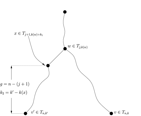
Figure 1: An illustration of some key definitions from the proof of the upper bound of Theorem 1.1.

Now fix $v^{\prime}$. If $v^{\prime}\in\mathcal{X}$, then by (i), (ii) and (iii), we have

$$k(x)\leq 3a(j+1),\qquad k^{\prime}-k(w)\leq 3a(g+1)=3a(n-j)$$

and so

$$k_{1}+k_{2}\leq 3a(n-j),\qquad k_{1}\leq\min\bigl{(}3a(j+1),3a(g+1)\bigr{)}$$ (22)

and if $v\in\mathcal{X}$, then, with $j=j(v,v^{\prime})$, we have

$$W_{j}\geq\frac{j}{n}(m_{n}-1)+\cases{(-a),&\quad$\mbox{whatever the value of }j,$\vspace*{2pt}\cr\min(j,n-j)^{1/40},&\quad$\mbox{if }a^{40}\leq j\leq n-a^{40}.$}$$ (23)

Consider separately four ranges of $j$. First, if $n-a^{40}\leq j\leq n-1$, then for sufficiently large $n$, (22) implies that $k_{1}+k_{2}\leq 3a(n-j)$, so $F_{j}$ is deterministically at most

$$\sum_{l\leq 3a(n-j)}|T_{n-j,l}|=\sum_{l\leq 3a(n-j)}\pmatrix{{n-j+l-1}\vspace*{2pt}\cr{l}}\leq 3a^{41}(a^{40}+3a^{41})^{a^{40}}.$$

Hence, recalling that $a$ is now a fixed, large constant,

$$\sum_{n-a^{40}\leq j\leq n}F_{j}\ll 1.$$ (24)

Next, let $r=(2\log n)^{40}$. If $n-r<j\leq n-a^{40}$, then for $n$ sufficiently large, $j\geq n-j=g+1$, and (23) implies that in order to have $W_{n}^{\prime}\leq m_{n}$ we must have

$$\widetilde{W}_{g}\leq\frac{g+1}{n}m_{n}-g^{1/40}+1\leq g/e-g^{1/40}+2,$$

the second inequality holding for sufficiently large $n$. For fixed $k_{1}$, by Lemma 3.2 we thus have

$$\mathbb{E}\bigl{\{}|\{v^{\prime}\in\mathcal{X},j(v,v^{\prime})=j,k_{1}(v,v^{\prime})=k_{1}\}||v\in\mathcal{X}\bigr{\}} \leq \mathbb{E}T_{g}(g/e-g^{1/40}+2)$$

$$\ll \exp[-eg^{1/40}].$$

Using (22) to bound $k_{1}$ and summing over $j$ yields

$$\sum_{n-r<j\leq n-a^{40}}F_{j}\ll\sum_{a^{40}\leq g\leq r}a(g+1)\exp[-eg^{1/40}]\ll 1.$$ (25)

Next, suppose $r\leq j\leq n-r$. By (23), in order to have $W_{n}^{\prime}\leq m_{n}$, it must be that

$$\widetilde{W}_{g}\leq\frac{g+1}{n}m_{n}-\min(j,n-j)^{1/40}+1\leq\frac{g}{e}-\log n.$$

Since we also require $k_{1}(v,v^{\prime})\leq 3an$ by (22), we have $F_{j}\leq 3an\mathbb{E}T_{g}(g/e-\log n)\ll 1/n^{2}$ for this range of $j$, and, hence,

$$\sum_{r\leq j\leq n-r}F_{j}\ll\frac{1}{n}.$$ (26)

Finally, suppose $0\leq j\leq r$. Here $g\geq n-r-1=n+O((\log n)^{40})$, and since $L_{a}(v)$ holds by assumption, if $v\in\mathcal{X}$, then

$$W_{j}\geq\frac{j}{n}W_{n}-a>\frac{j}{n}m_{n}-(a+1).$$

For each integer $b\in[-(a+1),2\log n)$, let $E_{b}$ be the event that $W_{j}-(j/n)m_{n}\in[b,b+1)$. Also, let $E^{*}$ be the event that $W_{j}-(j/n)m_{n}\geq\lceil 2\log n\rceil$. The events $\{E_{b}\dvtx-(a+1)\leq b<2\log n\}$ and $E^{*}$ together partition the event $\{v^{\prime}\in\mathcal{F}_{j}(v)\}$, so by conditioning

$$\quad F_{j}\leq\max\Bigl{(}\mathbb{E}\{|\mathcal{F}_{j}||v\in\mathcal{X},E^{*}\},\max_{-(a+1)\leq b<2\log n}\mathbb{E}\{|\mathcal{F}_{j}||v\in\mathcal{X},E_{b}\}\Bigr{)}.$$ (27)

If $W_{j}\geq(j/n)m_{n}+2\log n$, then to have $v^{\prime}\in\mathcal{F}_{j}$, we must have $\widetilde{W}_{g}(v^{\prime})\leq g/e-\log n$ so, as in the case $r\leq j\leq n-r$, we have

$$\mathbb{E}\{|\mathcal{F}_{j}||v\in\mathcal{X},E^{*}\}\ll\frac{1}{n^{2}}.$$

Now suppose $W_{j}-(j/n)m_{n}\in[b,b+1]$, where $b$ is an integer satisfying $-a-1\leq b\leq 2\log n$. Note that if $b<(j^{1/40}-2)$ and $a^{40}\leq j\leq r$, then $\mathcal{F}_{j}(v)$ is necessarily empty due to $B_{a}(v)$, so for such $j$ and $b$, $\mathbb{E}\{|\mathcal{F}_{j}||v\in\mathcal{X},E_{b}\}=0$. For the rest, we further subdivide $\mathcal{F}_{j}$, writing $\mathcal{F}_{j,l}=\{v^{\prime}\in\mathcal{X},j(v,v^{\prime})=j,k_{1}(v,v^{\prime})=l\}$. By (22) we have

$$\mathbb{E}\{|\mathcal{F}_{j}||v\in\mathcal{X},E_{b}\}=\sum_{l\leq 3a(j+1)}\mathbb{E}\{|\mathcal{F}_{j,l}||v\in\mathcal{X},E_{b}\}.$$

Suppose additionally that $W^{\prime}_{j+1}(v^{\prime})-W^{\prime}_{j}(v^{\prime})\in[\Delta,\Delta+1]$, where $\Delta$ is a nonnegative integer. Since $W_{j}(v^{\prime})=W_{j}(v)$, in order to have $v^{\prime}\in\mathcal{F}_{j}$, by (i) we require

$$\widetilde{W}_{g}-\frac{g}{n}m_{n}\in[m_{n}/n-(b+\Delta+3),m_{n}/n-(b+\Delta)].$$

Since $0\leq m_{n}/n<1$ and, for $n$ sufficiently large, $m_{g}-1\leq(g/n)m_{n}\leq m_{g}$, this implies that, writing $\mathcal{I}=[-(b+\Delta+4),-(b+\Delta-1)]$, we must have

$$\widetilde{W}_{g}-m_{g}\in\mathcal{I}.$$

By (i) and (ii), we also require

$$\widetilde{W}_{i}\geq\frac{i}{n}W_{n}-b-\Delta-a-2\geq\frac{i}{g}m_{g}-b-\Delta-a-3\qquad(i\leq g).$$

This implies that for all $i\leq g$,

$$\widetilde{W}_{i}\geq\frac{i}{g}\widetilde{W}_{g}-\max(b+\Delta+a-3,a-2).$$

None of this depends on $l$, so for any $0\leq l\leq 3a(j+1)$, writing $m=\max(b+\Delta+a-3,a-2)$,

$$\mathbb{E}\{|\mathcal{F}_{j,l}||v\in\mathcal{X},E_{b}\}$$

$$\qquad\leq\mathop{\sum_{1\leq k_{2}\leq 3a(j+1)}}_{\Delta\geq 0}\mathbb{E}|\{v\in T_{g,k_{2}}\dvtx S(v)-m_{g}\in\mathcal{I},L_{m}(v)\}|$$

$$\qquad\leq\mathop{\sum_{1\leq k_{2}\leq 3a(j+1)}}_{\Delta\geq 0}\Bigl{(}\mathbb{E}\bigl{\{}T_{g,k_{2}}\bigl{(}m_{g}-(b+\Delta-1)\bigr{)}\bigr{\}}$$

$$\hskip 65.0pt\qquad{}\times\sup_{x\in\mathcal{I}}\mathbb{P}\{L_{m}(\mathbf{v}_{g,k_{2}})|W_{g}(\mathbf{v}_{g,k_{2}})=m_{g}+x\}\Bigr{)}$$

$$\qquad\ll\sum_{\Delta\geq 0}\mathbb{E}\bigl{\{}T_{g}\bigl{(}m_{g}-(b+\Delta-1)\bigr{)}\bigr{\}}\cdot j\cdot\frac{\max(b+\Delta+a-3,a-2)^{6}}{n}$$

$$\qquad\ll\sum_{\Delta\geq 0}ne^{-e(b+\Delta)}\cdot j\cdot\frac{\max(b+\Delta+a-3,a-2)^{6}}{n}$$

$$\qquad\ll je^{-eb}(a+|b|)^{6},$$

the third-to-last line by Lemma 4.4 and the second-to-last by Lemma 3.2. Summing over $0\leq l\leq 3a(j+1)$, it follows that

$$\mathbb{E}\{|\mathcal{F}_{j}||v\in\mathcal{X},E_{b}\}\ll j^{2}e^{-eb}(a+|b|)^{6}.$$

For $j\leq a^{40}$ this is $O(1)$ uniformly in $b$. When $j>a^{40}$ we also have $b\geq j^{1/40}-2$ and for such $j$, the above bound is $O(j^{3}e^{-ej^{1/40}})$. By (27) it follows that for such $0\leq j\leq r$,

$$F_{j}\ll\cases{1,&\quad$\mbox{if }j\leq a^{40},$\vspace*{2pt}\cr\max(n^{-2},j^{3}\exp(-ej^{1/40})),&\quad$\mbox{if }j>a^{40}.$}$$

Summing on $j$, we find that

$$\sum_{0\leq j\leq r}F_{j}\ll 1.$$ (28)

Together, (24)–(26) and (28) imply that for every $v\in T$,

$$\mathbb{E}[X\dvtx v\in\mathcal{X}]=O(1).$$

Combining this estimate with (20) and (6) shows that $\mathbb{P}\{X>0\}\gg 1$, and if $X>0$, then $M_{n}\leq m_{n}$, so there exists an absolute constant $\varepsilon>0$ such that for all $n$,

$$\mathbb{P}\{M_{n}\leq m_{n}\}\geq\varepsilon.$$

From here it is straightforward to show that $M_{n}\leq\widetilde{M}_{n}+O(1)$, and we now do so. The next two lemmas, taken from ford09pratt , are standard bounds for BRW. As the proofs are short, we include them here.

Lemma 6.1

For any BRW, positive integers $m,n$ and positive real numbers $M$, $N$,

$$\mathbb{P}\{M_{m+n}\geq M+N\}\leq\mathbb{E}\bigl{[}(\mathbb{P}\{M_{n}\geq N\})^{T_{m}(M)}\bigr{]}.$$

Suppose $M_{m+n}\geq M+N$ and $T_{m}(M)=k$. For each of these $k$ individuals, all of their descendants in generation $m+n$ are offset from their generation $m$ ancestor by at least $N$.

Lemma 6.2

Let $m,n$ be positive integers and let $M>0,\varepsilon>0$ be real. If $\mathbb{E}\{(1-\varepsilon)^{T_{m}(M)}\}<\frac{1}{2}$, then $\mathbb{P}\{M_{n}<\widetilde{M}_{n+m}-M\}\leq\varepsilon.$ In particular, the conclusion holds if $\mathbb{P}\{T_{m}(M)<1/\varepsilon\}\leq\frac{1}{5}$.

Let $q=\sup\{x\dvtx\mathbb{P}\{M_{n}<x\}<\varepsilon\}$; then $\mathbb{P}\{M_{n}<q\}\leq\varepsilon$. By Lemma 6.1,

$$\mathbb{P}\{M_{m+n}\geq M+q\}\leq\mathbb{E}\bigl{[}(\mathbb{P}\{M_{n}\geq q\})^{T_{m}(M)}\bigr{]}<\tfrac 12.$$

Therefore, $M+q\geq\widetilde{M}_{m+n}$, and, thus, $\mathbb{P}\{M_{n}<\widetilde{M}_{m+n}-M\}\leq\mathbb{P}\{M_{n}<q\}\leq\varepsilon$. To prove the second part, assume that $\mathbb{P}\{T_{m}(M)<1/\varepsilon\}\leq\frac{1}{5}$. Then

$$\mathbb{E}\bigl{\{}(1-\varepsilon)^{T_{m}(M)}\bigr{\}} \leq \mathbb{P}\biggl{\{}T_{m}(m)<\frac{1}{\varepsilon}\biggr{\}}+\biggl{(}1-\mathbb{P}\biggl{\{}T_{m}(M)<\frac{1}{\varepsilon}\biggr{\}}\biggr{)}(1-\varepsilon)^{1/\varepsilon}$$

$$\leq \frac{1}{5}+\frac{4}{5e}<\frac{1}{2}.\hskip 200.0pt\qed$$

Now take $A$ such that $\mathbb{P}\{T_{1}(A)<1/\varepsilon\}\leq\frac{1}{5}$. By Lemma 6.2,

$$\mathbb{P}\{M_{n}\leq\widetilde{M}_{n}-A\}\leq\mathbb{P}\{M_{n}\leq\widetilde{M}_{n+1}-A\}\leq\varepsilon$$

and, hence, $\widetilde{M}_{n}\leq M_{n}+A$, which completes the proof of the upper bound in Theorem 1.1.

7 Proof of Theorem 1.2

Let $a>1/e$ and $0<\eta<ae/2$. By Biggins’ analog of Chernoff’s inequality for the BRW (Big77, , Theorem 2), for large $r$ we have $\mathbb{P}\{T_{r}(ar)\leq(ae-\eta)^{r}\}\leq\frac{1}{5}$. Let $r_{0}$ be large enough that, in addition, $\widetilde{M}_{n+r}\geq\widetilde{M}_{n}+(1/e-\eta)r$ for all $r\geq r_{0}$ and all $n$ (such an $r_{0}$ exists by Theorem 1.1). Now fix $r\geq r_{0}$ and let $M=ar$, let $m=r$, and let $\varepsilon=(ae-\eta)^{-r}$. We then have $\mathbb{P}\{T_{m}(M)<1/\varepsilon\}\leq 1/5$, so for all $n$, by the preceding bound for $\widetilde{M}_{n+r}$ and by Lemma 6.2, we obtain that

$$\mathbb{P}\{M_{n}\leq\widetilde{M}_{n}-(a-1/e+\eta)r\}\leq\mathbb{P}\{M_{n}\leq\widetilde{M}_{n+r}-ar\}\leq(ae-\eta)^{-r}.$$

The first estimate follows with $c_{1}=\frac{\log(ae-\eta)}{(a-1/e+\eta)}$. Fix $a$, let $\eta\to 0$, then let $a\to 1/e$, so that $c_{1}\to e$. This proves the first part of Theorem 1.2.

For the second part, fix $0<\varepsilon<1/50$ and let $\delta=\varepsilon^{2}$, so that $\delta(1+\log((1-\varepsilon/5)/\delta))<\varepsilon/5$. Then choose $r_{0}$ sufficiently large that for all $r\geq r_{0}$, we have $(1-\varepsilon/5)r+2\lceil\log(2r)\rceil<r$, and for all $s\geq\log(2r_{0})$, we have $\mathbb{P}\{T_{s}(2s)\leq 4^{s}\}\leq e^{-1/\delta}$ (as in the first part, such an $r_{0}$ exists by (Big77, , Theorem 2)).

Recall that if $h\in\mathbb{N}^{1}=T_{1}$ is a child of the root in $T$, then $S(h)$ is $\operatorname{Gamma}(h)$ distributed. Thus, for any positive integer $r$, by a union bound

$$\mathbb{P}\bigl{\{}T_{1}\bigl{(}(1-\varepsilon/5)r\bigr{)}\leq\delta r-1\bigr{\}} \leq \sum_{h\leq\delta r}\mathbb{P}\{S(h)\geq(1-\varepsilon/5)r\}$$

$$= \sum_{h\leq\delta r}\frac{e^{-(1-\varepsilon/5)r}((1-\varepsilon/5)r)^{h}}{h!}$$

$$\leq e^{-(1-\varepsilon/5)r}e^{(1+\log((1-\varepsilon/5)/\delta))\delta r}$$

$$\leq e^{-(1-2\varepsilon/5)r},$$

the second-to-last inequality by Proposition 3.3.

Write $s=\lceil\log(2r)\rceil$, and let $E$ be the event that there are at least $4^{s}$ nodes in $T_{s+1}$ with displacement at most $(1-\varepsilon/5)r+2s<r$. If $T_{1}((1-\varepsilon/5)r)>\delta r$, then either $E$ occurs, or else for each $h\leq\lceil\delta r-1\rceil$, the number of $v\in T_{s+1}$ descending from $h\in T_{1}$ with $S(v)-S(h)\leq 2s$ is less than $4^{s}$. The latter event has probability less than $(e^{-(1/\delta)})^{\delta r-1}=e^{(1/\delta)-r}$. It follows that

$$\mathbb{P}\{E^{c}\}\leq e^{-(1-2\varepsilon/5)r}+e^{(1/\delta)-r}\leq e^{-(1-\varepsilon/2)r},$$

the last inequality holding for large $r$. Finally, if $M_{n}>\widetilde{M}_{n-(s+1)}+r$, then for each node $v\in T_{s+1}$ with $S(v)\leq(1-\varepsilon/5)r+2s$, for all $w\in T_{n}$ descending from $v$ we must have $S(w)-S(v)\geq\widetilde{M}_{n-(s+1)}$. If $E$ occurs, then there are at least $4^{s}\geq 2r$ such nodes $v$, and so

$$\mathbb{P}\bigl{\{}M_{n}>\widetilde{M}_{n-(s+1)}+r\bigr{\}}\leq e^{-(1-\varepsilon/2)r}+2^{-2r}<e^{-(1-\varepsilon)r},$$

the last inequality holding for large $r$. Since $\widetilde{M}_{n-(s+1)}\leq\widetilde{M}_{n}$, the second part of Theorem 1.2 is proved by letting $\varepsilon\to 0$.

References

(1){barticle}[mr]
\bauthor\bsnmAddario-Berry, \bfnmLouigi\binitsL. and \bauthor\bsnmReed, \bfnmBruce\binitsB.
(\byear2009).
\btitleMinima in branching random walks.
\bjournalAnn. Probab.
\bvolume37
\bpages1044–1079.
\biddoi=10.1214/08-AOP428, issn=0091-1798, mr=2537549
\bptokimsref
\endbibitem
(2){bmisc}[auto:STB—2012/04/30—08:06:40]
\bauthor\bsnmAïdékon, \bfnmE.\binitsE.
(\byear2011).
\bhowpublishedConvergence in law of the minimum of a branching random
walk. Available at arXiv:\arxivurl1101.1810v1 [math.PR].
\bptokimsref
\endbibitem
(3){barticle}[mr]
\bauthor\bsnmAïdékon, \bfnmElie\binitsE. and \bauthor\bsnmShi, \bfnmZhan\binitsZ.
(\byear2010).
\btitleWeak convergence for the minimal position in a branching
random walk: A
simple proof.
\bjournalPeriod. Math. Hungar.
\bvolume61
\bpages43–54.
\biddoi=10.1007/s10998-010-3043-x, issn=0031-5303, mr=2728431
\bptokimsref
\endbibitem
(4){bincollection}[mr]
\bauthor\bsnmAldous, \bfnmDavid\binitsD. and \bauthor\bsnmSteele, \bfnmJ. Michael\binitsJ. M.
(\byear2004).
\btitleThe objective method: Probabilistic combinatorial optimization and
local weak convergence.
In \bbooktitleProbability on Discrete Structures.
\bseriesEncyclopaedia Math. Sci.
\bvolume110
\bpages1–72.
\bpublisherSpringer, \baddressBerlin.
\bidmr=2023650
\bptokimsref
\endbibitem
(5){barticle}[mr]
\bauthor\bsnmBachmann, \bfnmMarkus\binitsM.
(\byear2000).
\btitleLimit theorems for the minimal position in a branching random
walk with
independent logconcave displacements.
\bjournalAdv. in Appl. Probab.
\bvolume32
\bpages159–176.
\biddoi=10.1239/aap/1013540028, issn=0001-8678, mr=1765165
\bptokimsref
\endbibitem
(7){barticle}[mr]
\bauthor\bsnmBiggins, \bfnmJ. D.\binitsJ. D.
(\byear1976).
\btitleThe first- and last-birth problems for a multitype age-dependent
branching process.
\bjournalAdv. in Appl. Probab.
\bvolume8
\bpages446–459.
\bidissn=0001-8678, mr=0420890
\bptokimsref
\endbibitem
(8){barticle}[mr]
\bauthor\bsnmBiggins, \bfnmJ. D.\binitsJ. D.
(\byear1977).
\btitleChernoff’s theorem in the branching random walk.
\bjournalJ. Appl. Probab.
\bvolume14
\bpages630–636.
\bidissn=0021-9002, mr=0464415
\bptokimsref
\endbibitem
(9){barticle}[mr]
\bauthor\bsnmBillingsley, \bfnmP.\binitsP.
(\byear1972).
\btitleOn the distribution of large prime divisors.
\bjournalPeriod. Math. Hungar.
\bvolume2
\bpages283–289.
\bidissn=0031-5303, mr=0335462
\bptokimsref
\endbibitem
(10){barticle}[mr]
\bauthor\bsnmBramson, \bfnmMaury\binitsM. and \bauthor\bsnmZeitouni, \bfnmOfer\binitsO.
(\byear2009).
\btitleTightness for a family of recursion equations.
\bjournalAnn. Probab.
\bvolume37
\bpages615–653.
\biddoi=10.1214/08-AOP414, issn=0091-1798, mr=2510018
\bptokimsref
\endbibitem
(11){barticle}[mr]
\bauthor\bsnmChauvin, \bfnmBrigitte\binitsB. and \bauthor\bsnmDrmota, \bfnmMichael\binitsM.
(\byear2006).
\btitleThe random multisection problem, travelling waves and the distribution
of the height of -ary search trees.
\bjournalAlgorithmica
\bvolume46
\bpages299–327.
\biddoi=10.1007/s00453-006-0107-7, issn=0178-4617, mr=2291958
\bptokimsref
\endbibitem
(12){barticle}[mr]
\bauthor\bsnmDevroye, \bfnmL.\binitsL.
(\byear1987).
\btitleBranching processes in the analysis of the heights of trees.
\bjournalActa Inform.
\bvolume24
\bpages277–298.
\biddoi=10.1007/BF00265991, issn=0001-5903, mr=0894557
\bptokimsref
\endbibitem
(13){barticle}[mr]
\bauthor\bsnmDonnelly, \bfnmPeter\binitsP. and \bauthor\bsnmGrimmett, \bfnmGeoffrey\binitsG.
(\byear1993).
\btitleOn the asymptotic distribution of large prime factors.
\bjournalJ. Lond. Math. Soc. (2)
\bvolume47
\bpages395–404.
\biddoi=10.1112/jlms/s2-47.3.395, issn=0024-6107, mr=1214904
\bptokimsref
\endbibitem
(14){barticle}[mr]
\bauthor\bsnmDvoretzky, \bfnmA.\binitsA. and \bauthor\bsnmMotzkin, \bfnmTh.\binitsT.
(\byear1947).
\btitleA problem of arrangements.
\bjournalDuke Math. J.
\bvolume14
\bpages305–313.
\bidissn=0012-7094, mr=0021531
\bptokimsref
\endbibitem
(15){barticle}[mr]
\bauthor\bsnmFord, \bfnmKevin\binitsK.,
\bauthor\bsnmKonyagin, \bfnmSergei V.\binitsS. V. and \bauthor\bsnmLuca, \bfnmFlorian\binitsF.
(\byear2010).
\btitlePrime chains and Pratt trees.
\bjournalGeom. Funct. Anal.
\bvolume20
\bpages1231–1258.
\biddoi=10.1007/s00039-010-0089-0, issn=1016-443X, mr=2746953
\bptokimsref
\endbibitem
(17){barticle}[mr]
\bauthor\bsnmHammersley, \bfnmJ. M.\binitsJ. M.
(\byear1974).
\btitlePostulates for subadditive processes.
\bjournalAnn. Probab.
\bvolume2
\bpages652–680.
\bidmr=0370721
\bptokimsref
\endbibitem
(18){bbook}[mr]
\bauthor\bsnmHarris, \bfnmTheodore E.\binitsT. E.
(\byear1963).
\btitleThe Theory of Branching Processes.
\bpublisherSpringer, \baddressBerlin.
\bidmr=0163361
\bptokimsref
\endbibitem
(19){barticle}[mr]
\bauthor\bsnmHu, \bfnmYueyun\binitsY. and \bauthor\bsnmShi, \bfnmZhan\binitsZ.
(\byear2009).
\btitleMinimal position and critical martingale convergence in branching
random walks, and directed polymers on disordered trees.
\bjournalAnn. Probab.
\bvolume37
\bpages742–789.
\biddoi=10.1214/08-AOP419, issn=0091-1798, mr=2510023
\bptokimsref
\endbibitem
(20){barticle}[mr]
\bauthor\bsnmKingman, \bfnmJ. F. C.\binitsJ. F. C.
(\byear1975).
\btitleThe first birth problem for an age-dependent branching process.
\bjournalAnn. Probab.
\bvolume3
\bpages790–801.
\bidmr=0400438
\bptokimsref
\endbibitem
(22){barticle}[mr]
\bauthor\bsnmPittel, \bfnmBoris\binitsB.
(\byear1994).
\btitleNote on the heights of random recursive trees and random -ary
search trees.
\bjournalRandom Structures Algorithms
\bvolume5
\bpages337–347.
\biddoi=10.1002/rsa.3240050207, issn=1042-9832, mr=1262983
\bptokimsref
\endbibitem
(23){barticle}[mr]
\bauthor\bsnmPratt, \bfnmVaughan R.\binitsV. R.
(\byear1975).
\btitleEvery prime has a succinct certificate.
\bjournalSIAM J. Comput.
\bvolume4
\bpages214–220.
\bidissn=0097-5397, mr=0391574
\bptokimsref
\endbibitem