Phase diagram of one-dimensional Hubbard-Holstein model at quarter-filling

Abstract

We derive an effective Hamiltonian for the one-dimensional Hubbard-Holstein model, valid in a regime of both strong electron-electron (e-e) and electron-phonon (e-ph) interactions and in the non-adiabatic limit ($t/\omega_{0}\leq 1$), by using a non-perturbative approach. We obtain the phase diagram at quarter-filling by employing a modified Lanczos method and studying various density-density correlations. The spin-spin AF (antiferromagnetic) interactions and nearest-neighbor repulsion, resulting from the e-e and the e-ph interactions respectively, are the dominant terms (compared to hopping) and compete to determine the various correlated phases. As e-e interaction $(U/t)$ is increased, the system transits from an AF cluster to a correlated singlet phase through a discontinuous transition at all strong e-ph couplings $2\leq g\leq 3$ considered. At higher values of $U/t$ and moderately strong e-ph interactions ($2\leq g\leq 2.6$), the singlets break up to form an AF order and then to a paramagnetic order all in a single sublattice; whereas at larger values of $g$ ($>2.6$), the system jumps directly to the spin disordered charge-density-wave (CDW) phase.

I Introduction:

A host of materials show evidence of e-ph interactions besides the expected e-e interactions. Angle-resolved photoemission spectroscopy (ARPES) experiments in cuprates photoem1 ; photoem3 , fullerides fullarene3 , and manganites lanzara2 indicate strong e-ph coupling. The interplay of e-e and e-ph interactions in these correlated systems leads to coexistence of or competition between various phases such as superconductivity, CDW, spin-density-wave (SDW) phases, or formation of novel non-Fermi liquid phases, polarons, bipolarons, etc. It is of particular interest to consider both the strong coupling regime, and the cross-over to the non-adiabatic limit where the lattice response is not slower in comparison to the heavy effective mass of the correlated electron system.

The simplest framework to analyze the effects of e-e and the concomitant e-ph interactions is offered by the Hubbard-Holstein model whose Hamiltonian is given by:

$$H_{hh}\! = \!-t\sum_{j\sigma}\left(c^{\dagger}_{j+1\sigma}c_{j\sigma}+{\rm H.c.}\right)+\omega_{0}\sum_{j}a_{j}^{\dagger}a_{j}$$ (1)

$$+g\omega_{0}\sum_{j\sigma}n_{j\sigma}(a_{j}+a_{j}^{\dagger})+U\sum_{j}n_{j\uparrow}n_{j\downarrow}.$$

Here, $n_{j\sigma}\equiv c_{j\sigma}^{\dagger}c_{j\sigma}$ with $c_{j\sigma}^{\dagger}$ and $a_{j}^{\dagger}$ being the creation operators at site $j$ for an electron with spin $\sigma$ and a phonon respectively. The Hamiltonian describes a tight-binding model with hopping amplitude $t$, a set of independent oscillators characterized by a dispersionless phonon frequency $\omega_{0}$, along with an onsite Coulomb repulsion of strength $U$ and an onsite electron-phonon interaction of strength $g$. The Holstein and the Hubbard models are recovered in the limits $U=0$ and $g=0$ respectively.

To gain insight into the rich physics of the Hubbard-Holstein model, several studies have been conducted (in one-, two-, and infinite-dimensions and at various fillings) by employing various approaches such as quantum Monte Carlo (QMC) qmc1 ; qmc3 ; qmc4 ; qmc5 ; qmc6 ; qmc7 , exact diagonalization exdiag1 ; exdiag2 ; exdiag4 , density matrix renormalization group (DMRG)dmrg , dynamical mean field theory (DMFT) dmft1 ; dmft2 ; dmft3 ; dmft4 ; dmft5 ; dmft6 ; dmft7 ; dmft8 , semi-analytical slave boson approximations slave_b1 ; slave_b2 ; slave_b3 , large-N expansion largeN2 , variational methods based on Lang-Firsov transformation LF , and Gutzwiller approximation GA .

In contrast to earlier approaches, we utilize a controlled analytic approach (that takes into account quantum phonons). Our method uses both the strong electron-phonon coupling limit $g>1$ and the strong Coulomb coupling limit $U/t>1$ to generate an effective $t-J$ model with displaced oscillators that can then be treated perturbatively, and generates longer-range interactions in an effective Hamiltonian. This model we then solve numerically for finite chains. We then obtain the phase diagram of the Hubbard-Holstein model at quarter-filling in one dimension.

Our effective Hamiltonian comprises of two dominant competing interactions – spin-spin AF interaction and nearest-neighbor (NN) electron repulsion. In addition, three types of hopping also result – the NN hopping with reduced band width, next-nearest-neighbor (NNN) hopping, and NN spin-pair $\sigma\bar{\sigma}$ hopping. As the e-e interaction $U/t$ is increased, the system sequentially transforms from an AF cluster phase to a correlated singlet phase followed by CDW phase(s) with (e-ph coupling $g$ dependent) accompanying spin order. The most interesting feature is that, at intermediate values of $U/t$ and for all strong e-ph couplings ($2\leq g\leq 3$) considered, a phase comprising of correlated NN singlets appears which suggests the possibility for superconductivity occurrence.

The paper is organized as fallows. In section II, we describe our non-perturbative approach for tackling strong e-ph interaction and derive the effective Hamiltonian; in section III, we discuss the region of parameter space for $U/t$, $\omega_{0}/t$, and $g$ where our derived results are applicable; next, different correlation functions are analyzed to obtain the various phases and the conditions for transitions between these phases are presented in section IV; then, in section V, we present the phase diagram; and in section VI our conclusions.

II Effective Hamiltonian

To get the effective Hubbard-Holstein Hamiltonian, we first carry out the well-known Lang-Firsov (LF) transformation lang $H^{LF}_{hh}=e^{T}H_{hh}e^{-T}$ where $T=-g\sum_{j\sigma}n_{j\sigma}(a_{j}-a_{j}^{\dagger})$. This transformation clothes the hopping electrons with phonons and displaces the simple harmonic oscillators. On rearranging the various terms, we get the following LF transformed Hamiltonian:

$$H^{LF}_{hh} = -t\sum_{j\sigma}(X_{j+1}^{\dagger}c_{j+1\sigma}^{\dagger}c_{j\sigma}X_{j}+{\rm H.c.})+\omega_{0}\sum_{j}a_{j}^{\dagger}a_{j}$$ (2)

$$-g^{2}\omega_{0}\sum_{j}n_{j}+(U-2g^{2}\omega_{0})\sum_{j}n_{j\uparrow}n_{j\downarrow},$$

where $X_{j}=e^{g(a_{j}-a_{j}^{\dagger})}$ and $n_{j}=n_{j\uparrow}+n_{j\downarrow}$. On noting that $X_{j}^{\dagger}X_{j}=1$, we can express, as shown below, our LF transformed Hamiltonian in terms of the composite fermionic operator $d_{j\sigma}^{\dagger}\equiv c_{j\sigma}^{\dagger}X_{j}^{\dagger}$ (i.e., a fermionic operator dressed with phonons):

$$H^{LF}_{hh}=-t\sum_{j\sigma}\left(d_{j+1\sigma}^{\dagger}d_{j\sigma}+{\rm H.c.}\right)+\omega_{0}\sum_{j}a_{j}^{\dagger}a_{j}$$

$$+(U-2g^{2}\omega_{0})\sum_{j}n_{j\uparrow}^{d}n_{j\downarrow}^{d}-g^{2}\omega_{0}\sum_{j}\left(n_{j\uparrow}^{d}+n_{j\downarrow}^{d}\right),$$ (3)

where $n_{j\sigma}^{d}=d_{j\sigma}^{\dagger}d_{j\sigma}$. The last term in Eq. (3) represents the polaronic energy and is a constant for a given number of particles and an associated set of parameters. Hence, we drop this term from now onwards.

The model represented by Eq. (3) is essentially the Hubbard Model for composite fermions with Hubbard interaction $U_{eff}=(U-2g^{2}\omega_{0})$ and can be directly converted to an effective $t-J$ model Hamiltonian in the limit of large $U_{eff}/t$. Thus, we get the effective $t-J$ Hamiltonian for composite fermions by projecting out double occupation.

$$H_{t-J} = P_{s}\left[-t\sum_{j\sigma}\left(d_{j+1\sigma}^{\dagger}d_{j\sigma}+{\rm H.c.}\right)+\omega_{0}\sum_{j}a_{j}^{\dagger}a_{j}\right.$$ (4)

$$+ \left.J\sum_{j}\left(\vec{S}_{j}\cdot\vec{S}_{j+1}-{n_{j}^{d}n_{j+1}^{d}\over{4}}\right)\right]P_{s},$$

where $n_{j}^{d}=n_{j\uparrow}^{d}+n_{j\downarrow}^{d}$, $J={4t^{2}\over{U-2g^{2}\omega_{0}}}$, $\vec{S}_{i}$ is the quantum mechanical spin operator for a spin $1/2$ fermion at site $i$, and $P_{s}$ is the operator that projects onto the singly occupied subspace. Next, we note that

$$X_{j+1}^{\dagger}X_{j} = e^{g(a_{j+1}^{\dagger}-a_{j+1})}e^{g(a_{j}-a_{j}^{\dagger})}$$ (5)

$$= e^{-g^{2}}e^{g(a_{j+1}^{\dagger}-a_{j}^{\dagger})}e^{-g(a_{j+1}-a_{j})}.$$

The effective $t-J$ Hamiltonian, given in Eq. (4), can be re-expressed in terms of fermionic operators as

$$H_{t-J}=H_{0}+H_{1},$$ (6)

where

$$H_{0} = -te^{-g^{2}}\sum_{j\sigma}P_{s}\left(c_{j+1\sigma}^{\dagger}c_{j\sigma}+{\rm H.c.}\right)P_{s}+\omega_{0}\sum_{j}a_{j}^{\dagger}a_{j}$$ (7)

$$+J\sum_{j}P_{s}\left(\vec{S}_{j}\cdot\vec{S}_{j+1}-{n_{j}n_{j+1}\over{4}}\right)P_{s},$$

and

$$\!\!\!\!\!H_{1} = -te^{-g^{2}}\!\sum_{j\sigma}P_{s}\!\left[c_{j+1\sigma}^{\dagger}c_{j\sigma}(Y_{+}^{j\dagger}Y_{-}^{j}-1)+{\rm H.c.}\right]\!P_{s}.$$ (8)

Here, we have separated the Hamiltonian into (i) an itinerant electronic system represented by $H_{0}$ containing nearest-neighbor hopping with a reduced amplitude ($te^{-g^{2}}$), electronic interactions, and no electron-phonon interaction; and (ii) the remaining part $H_{1}$ which is a perturbation and corresponds to the composite fermion terms containing the e-ph interaction with $Y^{j}_{\pm}\equiv e^{\pm g(a_{j+1}-a_{j})}$.

II.1 Perturbation Theory

The unperturbed Hamiltonian $H_{0}$ is characterized by the eigenstates $|n,m\rangle\equiv|n\rangle_{el}\otimes|m\rangle_{ph}$ and corresponding eigenenergies $E_{n,m}=E_{n}^{el}+E_{m}^{ph}.$ On noting that the first-order perturbation term is zero (i.e., $\langle 0,0|H_{1}|0,0\rangle=0$), we proceed to calculate the second-order perturbation term $E^{(2)}=\sum\limits_{n,m}{{\langle 0,0|H_{1}|n,m\rangle\langle n,m|H_{1}|0,0\rangle}\over{E_{0,0}-E_{n,m}}}$ in a manner similar to that introduced in Ref. sdadys, . Now, $\Delta E_{m}=E_{m}^{ph}-E_{0}^{ph}$ is a positive integral multiple of $\omega_{0}$ and $E_{n}^{el}-E_{0}^{el}\sim te^{-g^{2}}\equiv t_{eff}$. In the narrow band limit, that $t_{eff}\ll\omega_{0}\ll U_{eff}$, we get the corresponding second-order perturbation term in the effective Hamiltonian for the polarons to be (see Appendix A for details):

$$H^{(2)}=\sum\limits_{m}{{{}_{ph}\!\langle 0|H_{1}|m\rangle_{ph}\times{{}_{ph}\!\langle m|H_{1}|0\rangle_{ph}}}\over{-\Delta E_{m}}}.$$ (9)

Evaluation of $H^{(2)}$ leads to the following expression:

$$H^{(2)} = \sum\limits_{j\sigma\sigma^{{}^{\prime}}}P_{s}\left[V\left(c_{j+1\sigma}^{\dagger}c_{j\sigma}c_{j\sigma^{{}^{\prime}}}^{\dagger}c_{j+1\sigma^{{}^{\prime}}}+c_{j\sigma}^{\dagger}c_{j+1\sigma}c_{j+1\sigma^{{}^{\prime}}}^{\dagger}c_{j\sigma^{{}^{\prime}}}\right)\right.$$ (10)

$$+ \!t_{2}\left(c_{j-1\sigma}^{\dagger}c_{j\sigma}c_{j\sigma^{{}^{\prime}}}^{\dagger}c_{j+1\sigma^{{}^{\prime}}}+c_{j+1\sigma}^{\dagger}c_{j\sigma}c_{j\sigma^{{}^{\prime}}}^{\dagger}c_{j-1\sigma^{{}^{\prime}}}\right.$$

$$+ \left.\left.c_{j\sigma}^{\dagger}c_{j+1\sigma}c_{j-1\sigma^{{}^{\prime}}}^{\dagger}c_{j\sigma^{{}^{\prime}}}+c_{j\sigma}^{\dagger}c_{j-1\sigma}c_{j+1\sigma^{{}^{\prime}}}^{\dagger}c_{j\sigma^{{}^{\prime}}}\right)\right]P_{s},$$

where $V=(2f_{1}+f_{2})t_{eff}^{2}/\omega_{0}$ and $t_{2}=f_{1}t_{eff}^{2}/\omega_{0}$ with $f_{1}=\sum\limits_{n=1}^{\infty}\frac{g^{2n}}{n!n}$ and $f_{2}=\sum\limits_{n,m=1}^{\infty}\frac{g^{2(m+n)}}{n!m!(m+n)}$. The value of $f_{1}$ and $2f_{1}+f_{2}$ can be approximated for large value of $g$ as $e^{g^{2}}/g^{2}$ and $e^{2g^{2}}/{2g^{2}}$ respectively. But in numerical simulation we have calculated the value of $f_{1}$ and $f_{2}$ by summing over the actual series.

Finally, to calculate each term in Eq. (10), we must project out the double occupancy. We do this projection by replacing every fermionic operator $c_{j\sigma}$ with the fermionic operator $c_{j\sigma}(1-n_{j\bar{\sigma}})$ (see Appendix B for details).

II.2 Effective Electronic Hamiltonian

The effective Hamiltonian, after averaging over the phononic degrees of freedom, is given by

$$H_{hh}^{eff} \cong -t_{eff}\sum\limits_{j\sigma}P_{s}\left(c_{j+1\sigma}^{\dagger}c_{j\sigma}+{\rm H.c.}\right)P_{s}+J\sum\limits_{j}P_{s}\left(\vec{S}_{j}\cdot\vec{S}_{j+1}-\frac{1}{4}n_{j}n_{j+1}\right)P_{s}$$ (11)

$$-\frac{t^{2}}{2g^{2}\omega_{0}}\sum\limits_{j\sigma}(1-\!\!n_{j+1\bar{\sigma}})(1-\!n_{j\bar{\sigma}})(n_{j\sigma}-n_{j+1\sigma})^{2}$$

$$-\frac{t^{2}e^{-g^{2}}}{g^{2}\omega_{0}}\sum\limits_{j\sigma}(1-n_{j+1\bar{\sigma}})(1-n_{j\bar{\sigma}})(1-n_{j-1\bar{\sigma}})\left[c_{j+1\sigma}^{\dagger}(1-2n_{j\sigma})c_{j-1\sigma}+{\rm H.c.}\right]$$

$$-\frac{t^{2}e^{-g^{2}}}{g^{2}\omega_{0}}\sum\limits_{j\sigma}(1-n_{j+1\bar{\sigma}})(1-n_{j-1\sigma})\left[c_{j\sigma}^{\dagger}c_{j+1\sigma}c_{j-1\bar{\sigma}}^{\dagger}c_{j\bar{\sigma}}+{\rm H.c.}\right].$$

Here, we have approximated the coefficients as $V\simeq t^{2}/{2g^{2}\omega_{0}}$ and $t_{2}\simeq t^{2}e^{-g^{2}}/{g^{2}\omega_{0}}$ which is valid for large values of $g$. The operator form of the last three terms in Eq. (11) can be visualized by considering different hopping processes depicted in Fig. 1. The third term in Eq. (11) depicts the process where an electron hops to its neighboring site [see Figs. 1(a) and 1(b)] and returns back. These two processes add up to the term $(n_{j\sigma}-n_{j+1\sigma})^{2}$ whose expansion yields the NN repulsion term $2n_{j\sigma}n_{j+1\sigma}$. The fourth term is composed of the two hopping processes shown in Figs. 1(c) and 1(d). Fig. 1(c) represents a double hopping process where a spin $\sigma$ particle hops first to its NN site and then to its NNN site. Contrastingly, Fig. 1(d) depicts the sequential process involving a pair of spin $\sigma$ electrons where an electron at site $j$ hops to its neighboring site $j+1$ followed by another electron at site $j-1$ hopping to site $j$. This sequential process may be called $\sigma\sigma$ pair hopping. The fifth term corresponds to Fig. 1(e) and represents a hopping process similar to that shown in Fig. 1(d) but involving a pair of electrons with opposite spins $\bar{\sigma}\sigma$. The additional factors $(1-n_{j+1\bar{\sigma}})(1-n_{j\bar{\sigma}})$, $(1-n_{j+1\bar{\sigma}})(1-n_{j\bar{\sigma}})(1-n_{j-1\bar{\sigma}})$, and $(1-n_{j+1\bar{\sigma}})(1-n_{j-1\sigma})$ appearing respectively in the third, fourth, and fifth terms in Eq. (11) represent projecting out double-occupancy at a site. The detailed derivation of these projected terms is given in Appendix B.

The coefficients of the last three terms in Eq.(11) (i.e., $t^{2}/{2g^{2}\omega_{0}}$ and $t^{2}e^{-g^{2}}/{g^{2}\omega_{0}}$), obtained from second order perturbation theory, are explained with the help of schematic diagrams shown in Fig. 2. We consider two distinct time scales for electronic hopping processes between two adjacent sites: (i) $\sim t_{eff}^{-1}$ associated with either full distortion of the lattice ions to form a small polaronic potential well (of energy $-g^{2}\omega_{0}$) or full relaxation from the small polaronic distortion and (ii) $\sim t^{-1}$ during which negligible distortion/relaxation of lattice ions occurs. The upper process in Fig. 2(a) [schematically representing the distortion for hopping sequence in Fig. 1(a)] shows the process in which an electron goes to its right neighbouring site and comes back. The intermediate state has energy $+g^{2}\omega_{0}$ and corresponds to fully distorted site $j$ but without the electron and neighbouring site $j+1$ containing the electron but without lattice distortion. To go from the intermediate state to the final one, the electron at site $j+1$ hops back to the original site $j$ without any new distortion taking place. Thus, the initial, the intermediate, and the final states all have identical lattice distortions. Hence, the hopping times for both these processes is $t^{-1}$. Then, from second order perturbation theory, the numerator of the coefficient is $t^{2}$ while the denominator (which is energy difference between the intermediate and the initial states) becomes $2g^{2}\omega_{0}$ leading to the coefficient $\frac{t^{2}}{2g^{2}\omega_{0}}$. The same coefficient results from the process in which an electron goes to its left neighbouring site and comes back as depicted by the lower process in Fig. 2(a). Thus the upper and lower processes in Fig. 2(a) both yield the same coefficient $\frac{t^{2}}{2g^{2}\omega_{0}}$.

The coefficient of the fourth term $t^{2}e^{-g^{2}}/{g^{2}\omega_{0}}$ corresponds to the schematic distortion processes shown in Figs. 2(b) and 2(c) with the pertinent hopping processes being depicted in Figs. 1(c) and 1(d) respectively. For the process where one electron at site $j-1$ consecutively hops to its NN site $j$ and then to NNN site $j+1$, the intermediate states which give dominant contributions are shown in Fig. 2(b). After the electron hops from site $j-1$ to site $j$, the upper intermediate state in Fig. 2(b) has the same lattice distortion as the initial state. On the other hand, again in the upper intermediate state in Fig. 2(b), when the electron makes the next hop from site $j$ to $j+1$ to produce the final state, there is a distortion at site $j+1$ with a concomitant relaxation at the initial site $j-1$. Hence the coefficient contribution, from the hopping process involving the upper intermediate state in Fig. 2(b), becomes $t\times te^{-g^{2}}/2g^{2}\omega_{0}$. Alternately, after the electron hops from site $j-1$ to site $j$, the initial state may lead to the lower intermediate state in Fig. 2(b) where the distortion at site $j-1$ is completely relaxed while site $j+1$ gets distorted simultaneously so that the intermediate and the final states have identical lattice distortions. This process too yields a coefficient contribution of $te^{-g^{2}}\times t/2g^{2}\omega_{0}$. The other six possible intermediate states (corresponding to the remaining possibilities of full distortion/relaxation at the three sites) each give $\sim t^{2}e^{-2g^{2}}$ in the numerator and hence we ignore them.

The coefficient of $\sigma\sigma$ or $\bar{\sigma}\sigma$ pair hopping [depicted by Figs. 1(d) and 1(e) respectively] can be derived from Fig. 2(c) which schematically represents the dominant contributions. The hopping process in Fig. 2(c), with upper (lower) intermediate state, represents sequential hopping where an electron at site $j$ hops to $j+1$ and produces the following changes: site $j+1$ is undistorted (distorted), $j-1$ distortion is unchanged (relaxed), and $j$ remains distorted. The hopping time for the first hop is $1/t$ ($1/t_{eff}$) and the change in energy between intermediate and initial states is $2g^{2}\omega_{0}$. Next, the electron at site $j-1$ hops to $j$ with site $j-1$ relaxing (remaining undistorted) and site $j+1$ getting (remaining) distorted. The second hop occurs in time $1/t_{eff}$ ($1/t$). Thus the $\sigma\sigma$ or $\bar{\sigma}\sigma$ pair hopping process, involving the two dominant intermediate processes of Fig. 2(c), yields the coefficient $t^{2}e^{-g^{2}}/g^{2}\omega_{0}$.

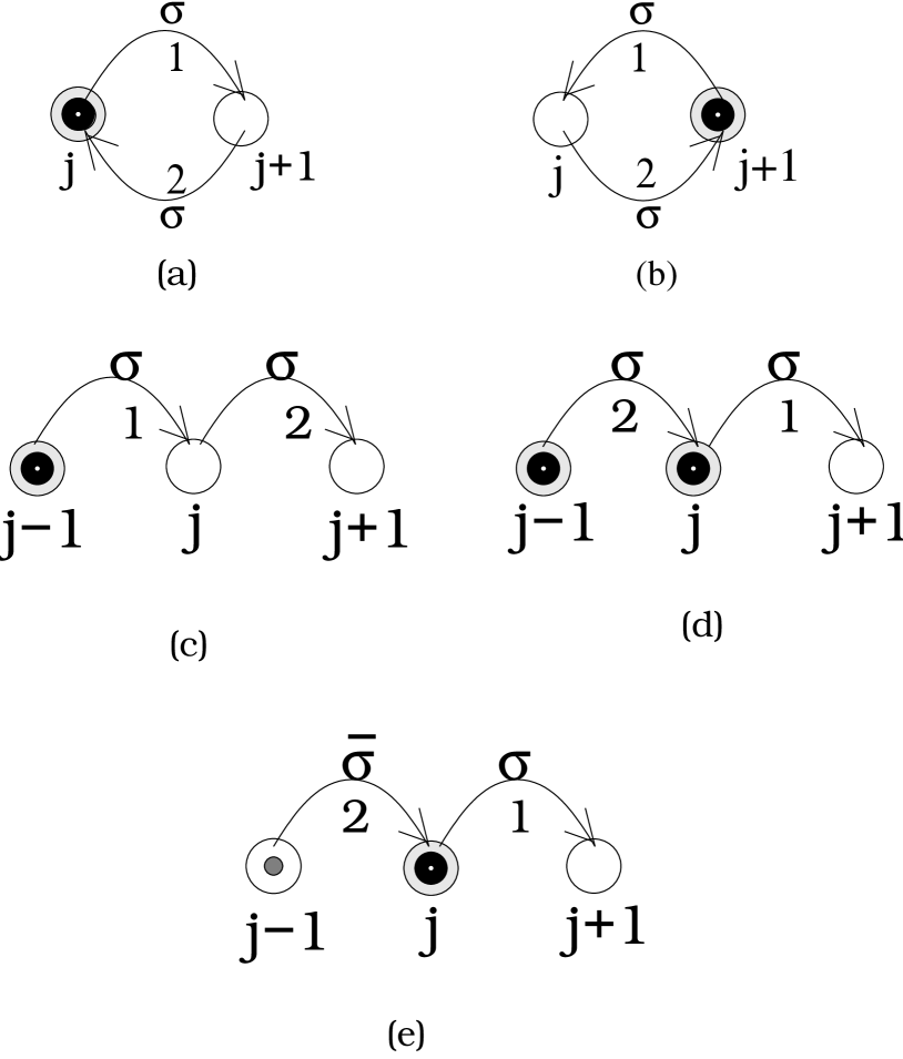
Figure 1: Different hopping processes contributing to second order perturbation theory are: (a) $c_{j\sigma}^{\dagger}c_{j+1\sigma}c_{j+1\sigma}^{\dagger}c_{j\sigma}$; (b) $c_{j+1\sigma}^{\dagger}c_{j\sigma}c_{j\sigma}^{\dagger}c_{j+1\sigma}$; (c) $c_{j+1\sigma}^{\dagger}c_{j\sigma}c_{j\sigma}^{\dagger}c_{j-1\sigma}$; (d) $c_{j\sigma}^{\dagger}c_{j-1\sigma}c_{j+1\sigma}^{\dagger}c_{j\sigma}$; and (e) $c_{j\bar{\sigma}}^{\dagger}c_{j-1\bar{\sigma}}c_{j+1\sigma}^{\dagger}c_{j\sigma}$. Here, empty circles correspond to sites with no electrons while circles with big and small dots inside correspond to sites with spin $\sigma$ and spin $\bar{\sigma}$ electrons respectively. The numbers $1$ and $2$ indicate the order of hopping.

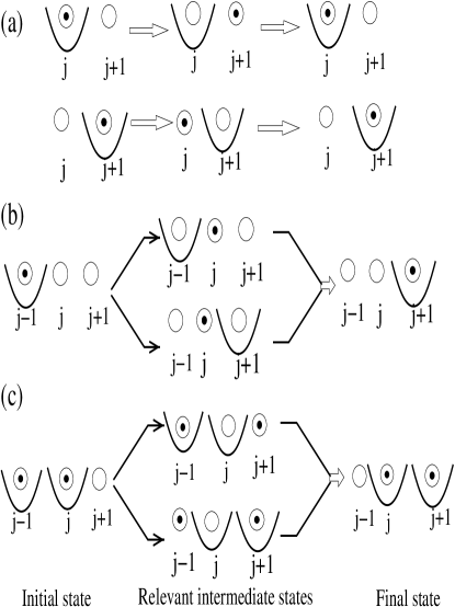
Figure 2: Schematic representation of the hopping processes considered in Fig. 1 with intermediate states giving the dominant contributions. Here empty circles correspond to empty sites, while circles with small dots indicate particle positions. Parabolic curve at a site depicts full distortion of the lattice ions at that site with corresponding energy $-g^{2}\omega_{0}$ ($+g^{2}\omega_{0}$) if the electron is present (absent) at that site.

III Region of validity of our theory

Our theory has three dimensionless parameters – Hubbard interaction $U/t$, adiabaticity $t/\omega_{0}$, and electron-phonon interaction strength $g$. An increase in $U/t$, while keeping fixed other dimensionless parameters, will decrease only the spin Heisenberg AF interaction $J=\frac{4t^{2}}{U-2g^{2}\omega_{0}}$ in the effective Hamiltonian of Eq. (11). Furthermore, an increase in $g$ produces an increase in $J$, a decrease in $V$, and also a decrease in all the various hopping (i.e., NN hopping, double hopping, and $\sigma\bar{\sigma}$ pair hopping) coefficients in Eq. (11).

For large values of $g$, the coefficients of NN hopping, NNN hopping, $(\sigma\bar{\sigma})$ pair hopping terms contain $e^{-g^{2}}$ and hence are small compared to NN repulsion $V$ and spin interaction $J$. Thus, unlike the usual $t-J$ model, here the spin-spin interaction term dominates over the hopping. Our model basically describes the competition between spin interactions and NN repulsion with the hopping being a small perturbation. By varying the dimensionless parameters in our model, the relative importance of $J$ and $V$ terms can be changed. When the effect of $J$ dominates over that of $V$, we expect formation of an AF cluster. On the other hand, when NN repulsion is larger than spin interaction, the electrons tend to get separated which can lead to different interesting phases.

For our theory to be valid, the following criterion need to be satisfied: (a) the dimensionless effective Hubbard interaction $U_{eff}/t\gg 1$ so that Eq. $(\ref{ai3})$ can be well approximated by the effective $t-J$ model given in Eq. $(\ref{ai5})$. Actually, for a one-dimensional Hubbard model, calculations avella show that $U_{eff}/t\gtrsim 8.0$ is sufficient to remove double occupancy; (b) NN electronic hopping $J_{1}$ and spin interaction $J$ should both be negligible compared to the phononic energy $\omega_{0}$ so as to make our perturbation theory valid; and (c) the small parameter sml_parameter1 ; sml_parameter2 of our perturbation theory $t/(g\omega_{0})$ should be kept as small as possible. Our calculations are done for $t/{g\omega_{0}}\leq 0.5$.

IV Results and Discussion

The half-filled case (i.e., average concentration of one electron per site) is not very interesting because, owing to exclusion of double occupancy, we have one electron in every site and consequently no hopping occurs. Here the system behaves like a Heisenberg AF chain with NN repulsion having no effect on electronic correlations. However, at quarter-filling there are enough vacancies for electrons so that, besides the spin interaction term, NN repulsion and different kinds of hopping in our model can contribute to a rich phase diagram. Therefore, we concentrate on the ground state properties at quarter-filling and analyze the different phases exhibited by our effective Hamiltonian in Eq. (11) and the quantum phase transitions (QPT) between these phases for large values of $g$, i.e., in the strong e-ph coupling limit.

We use a modified Lanczos algorithm dagatto to calculate the ground state. To get the basis states in the occupation number representation, we exclude double occupancy and permit only the remaining three possible electronic states on any site (i.e., ↑, ↓,  and no particle). The size of the resulting Hilbert space prohibits us from calculating the ground state for large systems. For example, the number of basis states for 16 sites with 8 electrons (4↑, 4↓) is ${}^{16}C_{8}\times^{8}C_{4}=900900$ which is quite large but manageable for calculating the ground state. But for 20 sites with 10 electrons (5↑, 5↓), the calculation of ground state requires ${}^{20}C_{10}\times^{10}C_{5}$ basis states which is prohibitive.

We find evidence for several different types of phases depending on parameter values. Because there is a tendency to form phase separated clusters, various methods are used to identify the phases. To characterize phase separation, we use a “$n-$particle normalized clustering probability” parameter NCP(n) (defined precisely in Appendix C) which actually measures the normalized probability of $n-$electron clusters in the ground state of the system. However, NCP(n) does not tell the number of $\uparrow$ and $\downarrow$ electrons or their arrangement in the cluster. To determine the different phases, we need to employ additional measures of ordering such as spin-spin correlation functions, structure factor, etc.

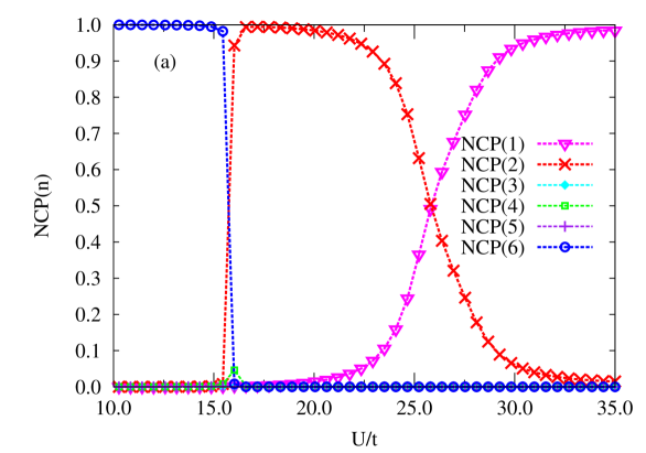
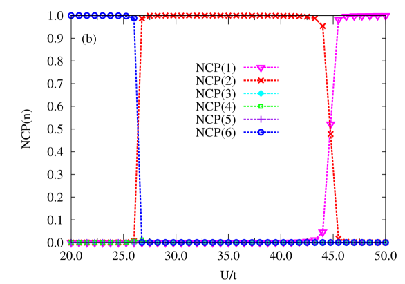
Figure 3: (Color online) n-particle normalized clustering probability [NCP(n)] for number of sites =12, number of electrons = 6 ($3\uparrow,3\downarrow$), $t/\omega_{0}=1.0$, and when (a) $g=2.2$ and (b) $g=2.8$.

IV.1 AF Cluster to Correlated Singlets Transition

Our numerical calculations were done for $t/\omega_{0}=1.0$ and $t/\omega_{0}=0.5$. Since the results are similar for the two values of $t/\omega_{0}$ considered, here we report only the calculations for $t/\omega_{0}=1.0$. By varying $g$ and $U/t$, we change the relative importance of $J$ and $V$ terms and get the different phases of the system.

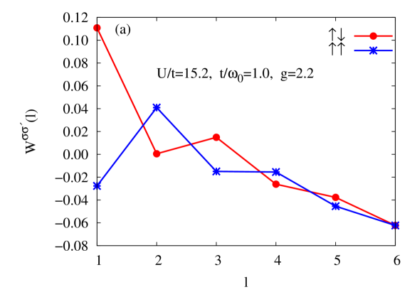
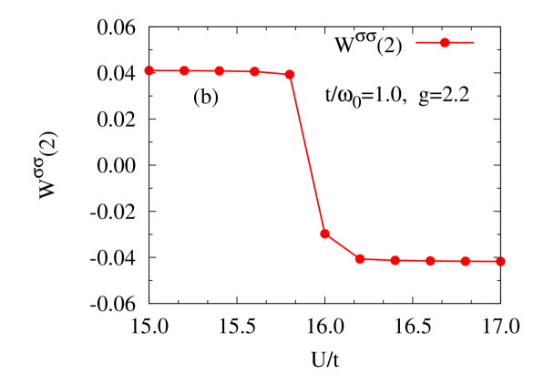
Figure 4: (Color online) Plot of the correlation functions (a) $W^{\sigma\sigma^{\prime}}(l)$ portraying an AF cluster for $U/t=15.2$, $t/\omega_{0}=1.0$, and $g=2.2$; and (b) $W^{\sigma\sigma}(2)$ versus $U/t$ again for $t/\omega_{0}=1.0$ and $g=2.2$.

It is clear from Fig. 3(a) that, for $t/\omega_{0}=1.0$ and $g=2.2$, for values of $U/t$ up to about 15.6 the NCP(6) $\approx 1.0$ which implies that all the particles in the system form a single cluster. This is because the effect of spin interaction dominates over the NN repulsion. But upon increasing $U/t$ further, the system undergoes a first-order QPT with NCP(6) discontinuously dropping to almost a zero value and NCP(2) concomitantly jumping abruptly to a value close to $1$. The value of NCP(2) remains close to 1 up to $U/t\approx 20.0$. Interestingly, for n=1,3,4,5 particles, NCP(n) remains almost zero up to $U/t\approx 23.0$. For all values of $g$ in the range $2\leq g\leq 3$, when $U/t$ is increased, the system transits discontinuously from a single cluster to a phase comprising of pairs of particles. This is verified for $g=2.8$ as well in Fig. 3$(b)$. Moreover, we notice that the correlated pairs phase persists over a broader window of $U/t$ values when $g$ is larger. In fact, for all the system sizes considered (i.e., number of sites N = 8, 12, and 16), we find that the systems manifest a first-order QPT from an AF cluster of size N/2 to a correlated singlet phase as $U/t$ increases.

Although Fig. 3 demonstrates the QPT clearly, it does not give information about the structure/order of the phases. We will confirm the AF order by analyzing the correlation between density fluctuations of spins ($\sigma$ and $\sigma^{\prime}$ separated by a distance $l$) through the correlation function $W^{\sigma\sigma^{\prime}}(l)={1\over{N}}\sum\limits_{j}\langle{n_{j}^{\sigma}n_{j+l}^{\sigma^{\prime}}}\rangle-\langle n_{j}^{\sigma}\rangle\langle n_{j+l}^{\sigma^{\prime}}\rangle$ with $N$ being the system size. Here $\langle n_{j}^{\sigma}\rangle$ is the filling factor which for quarter-filling is $0.25$. Fig. 4(a) shows the correlation functions $W^{\sigma\sigma^{\prime}}(l)$ for $U/t=15.2$, $t/\omega_{0}=1.0$, and $g=2.2$, i.e., away from the transition. This clearly shows that in the cluster, the dominant arrangement of the spins is antiferromagnetic with correlation decreasing with distance $l$. This is expected because of the transverse spin fluctuation term in the Heisenberg interaction. Next, in Fig. 4$(b)$, $W^{\uparrow\uparrow}(2)$ is shown as $U/t$ is varied. There is a sudden jump in $W^{\uparrow\uparrow}(2)$ indicating that the system breaks up into two-particle clusters from an AF cluster.

Now, we need to determine the structure of the phase with NCP(2) $\approx 1.0$ in Fig. 3. The important question is: what is the nature of the pairs? The answer lies in the correlation function plot $W^{\sigma\sigma^{\prime}}(l)$ shown in Fig. (5) for $U/t=18.0$ (i.e., deep inside the phase). Here, we see that the value of $W^{\uparrow\uparrow}(1)$ is approximately its minimum possible value of $-0.0625$ which occurs when ${1\over{N}}\sum\limits_{j}\langle{n_{j}^{\sigma}n_{j+1}^{\sigma}}\rangle\approx 0.0$. This means that each pair is made up of two opposite spin electrons. Furthermore, $W^{\uparrow\downarrow}(1)=0.0625$ in Fig. (5) which is expected because $W^{\uparrow\downarrow}(1)$ should have a calculated value of $0.25\times 0.5-0.0625=0.0625$. Next, we notice that, for $l\geqslant 2$, $W^{\uparrow\downarrow}(l)$ and $W^{\uparrow\uparrow}(l)$ have the same values. This means that, given a $\sigma\bar{\sigma}$ pair, we get not only an $\uparrow\downarrow$ pair at a distance $l$ with a certain probability but also a $\downarrow\uparrow$ pair at the same distance and with the same probability. Thus a pair of opposite spin electrons located at sites $j$ and $j+1$ can either be a singlet or a triplet with $S^{z}_{total}=0$. When acted upon by the operator $S_{j}^{+}S_{j+1}^{-}+S_{j}^{-}S_{j+1}^{+}$, the singlet state yields eigenvalue -1 while the $S^{z}_{total}=0$ triplet state gives +1. Thus to know the nature of the spin pairs in the system, we have calculated the quantity $\sum\limits_{j}\langle(S_{j}^{+}S_{j+1}^{-}+S_{j}^{-}S_{j+1}^{+})\rangle$ and obtained a value very close to $-3.0$ for $6$ electrons ($3\uparrow$ and $3\downarrow$) for the whole range of $16.0\lesssim U/t\lesssim 22.5$. Thus the phase is entirely made up of singlets. In Fig. 5, we also notice that $W^{\uparrow\downarrow}(l)$ and $W^{\uparrow\uparrow}(l)$ show a peak at $l=4$ and slightly lesser values for $l=3$ and $l=5$ which is indicative of a CDW. We call this phase a correlated singlet phase. A detailed analysis of this phase at various filling factors will be presented elsewhere srsypbl2 .

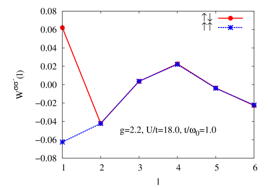
Figure 5: (Color online) Plot of correlation functions $W^{\sigma\sigma^{\prime}}(l)$ in the correlated singlet phase for $g=2.2$, $U/t=18.0$, and $t/\omega_{0}=1.0$.

The transition from an AF cluster to correlated singlets can be explained by invoking Bethe ansatz results. Suppose we have a Hamiltonian of the type $H=\tilde{J}\sum\limits_{j}S_{j}.S_{j+1}+\tilde{V}\sum\limits_{j}n_{j}n_{j+1}$. Then, for the cluster regime, Bethe ansatz yields energy/site $=-0.443\tilde{J}+2\frac{\tilde{V}}{2}$ where as for separated singlets in the correlated singlet phase the energy/site $=-\tilde{J}(0.375)+\frac{\tilde{V}}{2}$. Thus the cluster regime prevails when $-0.443\tilde{J}+\tilde{V}\leq-\tilde{J}(0.375)+\frac{\tilde{V}}{2}$, i.e., $\tilde{V}\leq 0.136\tilde{J}$. Now, if in Eq. (11) we neglect all the hopping terms (which is true for large $g$), based on the above analysis, we obtain the condition for existence of the cluster phase to be $(2V-\frac{J}{4})\lesssim 0.136J$ or equivalently $U/t\lesssim 3.544g^{2}\omega_{0}/t$. This condition gives a very good estimation of the actual phase boundary in the phase diagram given in Fig. 6.

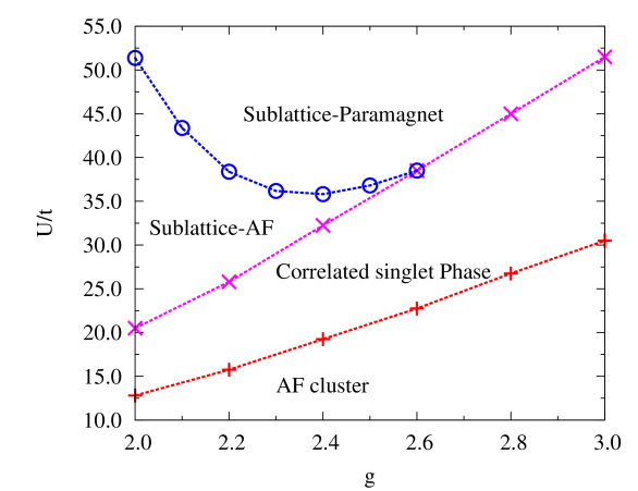
Figure 6: (Color online) The phase diagram of the Hubbard-Holstein model at quarter-filling in the $t/\omega_{0}=1.0$ plane.

IV.2 Transition from correlated singlets to spins in one sublattice

Here we discuss how, for a fixed $g$ and larger values of $U/t$, the correlated singlets break up into spins occupying only one sublattice . It is clear from Fig. 3(a) that this is a second-order phase transition at smaller values of $g$ (such as $g=2.2$) because NCP(1) [NCP(2)] increases [decreases] continuously as $U/t$ is raised. On the other hand, this transition tends towards first-order at larger values of $g$ [say $g=2.8$ as shown in Fig. 3(b)]. This transition can be explained as follows. As $U/t$ is increased, $J$ gets reduced and NN repulsion starts dominating over spin interaction leading to the break up of singlets and single spins separating out to occupy one sublattice only.

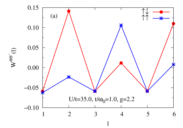
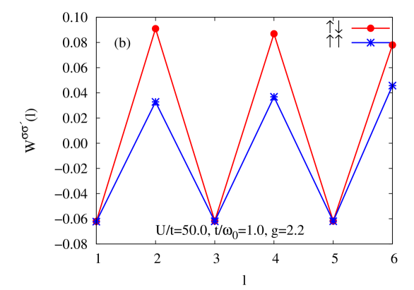
Figure 7: (Color online) Correlation functions $W^{\sigma\sigma^{\prime}}(l)$ at $t/\omega_{0}=1.0$, $g=2.2$, and for (a) $U/t=35.0$ depicting AF order in one sublattice; and for (b) $U/t=50.0$ displaying paramagnetic phase in one sublattice.

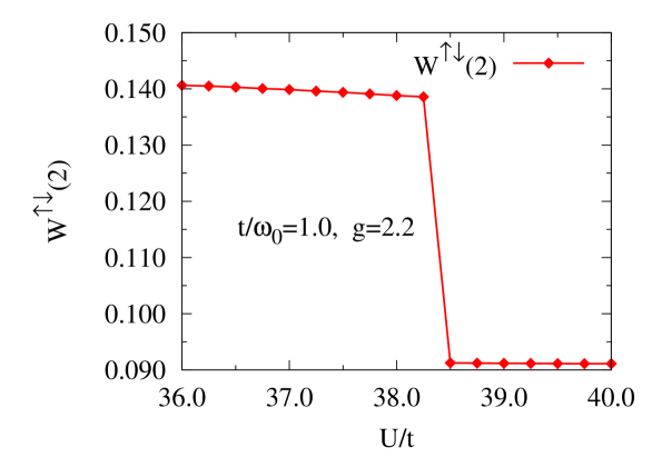
Figure 8: (Color online) Plot of the correlation function $W^{\uparrow\downarrow}(2)$ versus $U/t$.

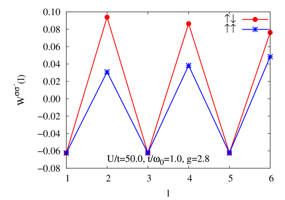
Figure 9: (Color online) Correlation functions $W^{\sigma\sigma^{\prime}}(l)$ depicting spin disorder in one sublattice for $U/t=50.0$, $t/\omega_{0}=1$, and $g=2.8$.

IV.2.1 Transitions at smaller $g$

For smaller values of $g$ (i.e., $2<g<2.6$), the QPT is not so sharp. In fact, for $g=2.2$ [as shown in Fig. 3(a)], the singlet pairs and separated single spins coexist in the range $23<U/t<30$. But when $U/t$ is increased further, almost all the pairs are broken and the electrons occupy one sublattice only. The correlation functions $W^{\uparrow\downarrow}(l)$ and $W^{\uparrow\uparrow}(l)$, depicted in Fig. 7$(a)$ for $U/t=35.0$ and $g=2.2$, show that the dominant structure has AF order in one sublattice (i.e, the spins arrange themselves as $\uparrow-\downarrow-\uparrow-\downarrow-...$). This can be surmised from the fact that the correlation functions $W^{\uparrow\downarrow}(l)$ and $W^{\uparrow\uparrow}(l)$ have dominant peaks at alternate even values of $l$. This spin arrangement is preferred by the system because it can gain energy due to AF interaction $(J)$ by virtual hopping to NN site and returning back. For very large values of $U/t$, the spin interaction strength $J$ becomes negligible and the electrons do not shown any spin order but still occupy only one sublattice. For this spin disordered situation, the values of $W^{\uparrow\downarrow}(l)$ and $W^{\uparrow\uparrow}(l)$ for the system under consideration [i.e., $12$ sites with $6$ electrons ($3\uparrow,3\downarrow$)] can be calculated as follows. The probability of getting one $\uparrow$ spin at any site, in a $12$-site system, is $0.25$. Now, as the spins are residing in only one sublattice, the probabilities of finding the remaining $3\downarrow$ and $2\uparrow$ electrons, in any of the remaining $5$ sites of the same sublattice, are $3/5$ and $2/5$ respectively. Hence, $W^{\uparrow\downarrow}(l)=0.25(3/5)-0.0625=0.0875$ and $W^{\uparrow\uparrow}(l)=0.25(2/5)-0.0625=0.0375$ for $l=2,4,6,8,10$. The above predicted values of the correlation functions $W^{\uparrow\downarrow}(l)$ and $W^{\uparrow\uparrow}(l)$ match well with the calculated values of these functions for $U/t=50.0,g=2.2$ as shown in Fig. 7(b). Another interesting point is that there is a first-order phase transition from AF order to paramagnetic order in one sublattice of the system as can be seen from the sudden jump (when $U/t$ is varied) in the correlation function $W^{\uparrow\downarrow}(2)$ depicted in Fig. 8.

IV.2.2 Transition for larger $g$ values

For $g\gtrsim 2.6$, when $U/t$ is increased, the correlated singlet phase transits to a paramagnetic state (in one sublattice) directly unlike the earlier case for smaller values of $g$ such as $g=2.2$ (see Fig. 9). This transition is of first-order character as shown in Fig.3$(b)$ where NCP(1) and NCP(2) show simultaneous sharp jumps in opposing directions.

V The Phase Diagram

The phase diagram of the Hubbard-Holstein model at quarter-filling in a twelve-site system for the $t/\omega_{0}=1.0$ plane is shown in Fig. 6. This is obtained by producing plots of NCP(n) versus $U/t$ for various values of $g$. Two such plots are shown in Fig. $(\ref{NCP})$ for values of $g=2.2$ and $g=2.8$. Then, from the NCP plots, we find phase transition points in the $g-U/t$ plane to obtain the phase diagram. Furthermore, using selective choice of parameter values, we also found that the qualitative features of the phase diagram remained the same even for the larger sixteen-site system.

In the phase diagram shown in Fig. 6, the system transits, for all values of $g$ in the range $2\leq g\leq 3$, from an AF cluster to a correlated singlet phase discontinuously when $U/t$ is increased. For $g\lesssim 2.6$, further increase in $U/t$ drives the system continuously from a correlated singlet phase to a single-sublattice AF phase. Next, at even higher values of $U/t$ and again for $g\lesssim 2.6$, the system jumps discontinuously from an AF order to a paramagnetic order in a single sublattice. Contrastingly, for $g\gtrsim 2.6$, the system transforms directly from a correlated singlet phase to a paramagnetic phase by a close-to-discontinuous jump.

VI Conclusions

By analyzing the probability of occurrence of different cluster sizes and by studying various correlation functions that result from our effective Hubbard-Holstein Hamiltonian, we deduced the ground state phase diagram (Fig. 6) at quarter-filling and in the non-adiabatic regime. In particular we find that strong electron-phonon coupling stabilizes a correlated singlet phase that is charge-density-wave like, which would be absent in the pure Hubbard model. Notice that this phase is also quite distinct from a Peierls-like ( “bond-order”) wave, being driven by onsite correlations alone. Our analysis and results should be of relevance to systems such as fullerides, lower-dimensional organic conductors, magnetic oxides, interfaces between oxides, where there is evidence for both strong Coulomb correlation as well as electron-phonon coupling. In higher dimensions, the concurrent NN spin-spin and NN repulsion interactions, could lead to even richer physics such as competition between or coexistence of charge ordering and superconductivity, non-Fermi liquid behavior, etc.

Appendix A

In this appendix, we will demonstrate the validity of Eq. (9). Let us assume a Hamiltonian of the form $H=H_{0}+H_{1}$ where the eigenstates of $H_{0}$ are all separable and are of the form $|n,m\rangle=|n\rangle_{el}\otimes|m\rangle_{ph}$ and $H_{1}$ is the electron-phonon interaction perturbation term of the form given in Eq. (8).

After a canonical transformation, we get

$$\tilde{H} = e^{S}He^{-S}$$ (12)

$$= \!\!H_{0}\!+\!H_{1}\!+\![H_{0}+H_{1},S]\!\!+\!\frac{1}{2}\left[[H_{0}\!+\!H_{1},S],S\right].$$

In the ground state energy, we know that the first-order perturbation term is zero. To eliminate the first-order term in $H_{1}$, we let $H_{1}+[H_{0},S]=0$. Consequently, we obtain

$$\langle n_{1},m_{1}|S|n_{2},m_{2}\rangle=-\frac{\langle n_{1},m_{1}|H_{1}|n_{2},m_{2}\rangle}{(E_{n_{1},m_{1}}-E_{n_{2},m_{2}})}.$$ (13)

We now assume that both the exponentially reduced electronic NN hopping energy $te^{-g^{2}}$ and the Heisenberg spin interaction energy $J$ are negligible compared to the phononic energy $\omega_{0}$ which is true for large values of $g$. This implies that $(E_{n_{1},m_{1}}-E_{n_{2},m_{2}})\simeq(E_{m_{1}}^{ph}-E_{m_{2}}^{ph})$. Then, Eq. (13) simplifies to the form

$${{}_{ph}\!\langle m_{1}|S|m_{2}\rangle_{ph}}=-\frac{{{}_{ph}\!\langle m_{1}|H_{1}|m_{2}\rangle_{ph}}}{(E_{m_{1}}^{ph}-E_{m_{2}}^{ph})}.$$ (14)

Now, using Eqs. (12) and (14), we obtain

$${{}_{ph}\!\langle m_{1}|\tilde{H}|m_{2}\rangle_{ph}} \simeq {{}_{ph}\!\langle m_{1}|H_{0}|m_{2}\rangle_{ph}}+\frac{1}{2}\sum_{\bar{m}}\left[~{}{{}_{ph}\!\langle m_{1}|H_{1}|\bar{m}\rangle_{ph}}~{}{{}_{ph}\!\langle\bar{m}|S|m_{2}\rangle_{ph}}-{{}_{ph}\!\langle m_{1}|S|\bar{m}\rangle_{ph}}~{}{{}_{ph}\!\langle\bar{m}|H_{1}|m_{2}\rangle_{ph}}\right]$$ (15)

$$\simeq {{}_{ph}\!\langle m_{1}|H_{0}|m_{2}\rangle_{ph}}+\frac{1}{2}\sum_{\bar{m}}{{{}_{ph}\!\langle m_{1}|H_{1}|\bar{m}\rangle_{ph}}~{}{{}_{ph}\!\langle\bar{m}|H_{1}|m_{2}\rangle_{ph}}}\left[\frac{1}{E_{m_{2}}^{ph}-E_{\bar{m}}^{ph}}+\frac{1}{E_{m_{1}}^{ph}-E_{\bar{m}}^{ph}}\right].$$

Appendix B Projection onto singly occupied subspace

In this appendix we evaluate each term in Eq. (10) by projecting out double occupancy. Every fermionic operator $c_{j\sigma}$ is subject to the replacement$c_{j\sigma}\rightarrow c_{j\sigma}(1-n_{j\bar{\sigma}})$ so as to incorporate the action of the single subspace projection operator $P_{s}$. In the first two terms of Eq. (10), the action of $P_{s}$ implies that spin index $\sigma=\sigma{{}^{\prime}}$. Thus, these first two terms correspond to the process where an electron hops to a neighboring site and comes back. Then, the projected form of the first term is evaluated to be

$$P_{s}\left(c_{j+1\sigma}^{\dagger}c_{j\sigma}P_{s}^{2}c_{j\sigma}^{\dagger}c_{j+1\sigma}\right)P_{s} = (1-n_{j+1\bar{\sigma}})c_{j+1\sigma}^{\dagger}c_{j\sigma}(1-n_{j\bar{\sigma}})(1-n_{j\bar{\sigma}})c_{j\sigma}^{\dagger}c_{j+1\sigma}(1-n_{j+1\bar{\sigma}})$$ (16)

$$= (1-n_{j+1\bar{\sigma}})c_{j+1\sigma}^{\dagger}c_{j\sigma}c_{j\sigma}^{\dagger}c_{j+1\sigma}(1-n_{j\bar{\sigma}}).$$

Similarly, for the second term we get

$$P_{s}c_{j\sigma}^{\dagger}c_{j+1\sigma}P_{s}^{2}c_{j+1\sigma}^{\dagger}c_{j\sigma}P_{s}=(1\!-\!\!\!n_{j+1\bar{\sigma}})c_{j\sigma}^{\dagger}c_{j+1\sigma}c_{j+1\sigma}^{\dagger}c_{j\sigma}(1\!-\!\!\!n_{j\bar{\sigma}}).$$ (17)

The above two processes are depicted in Figs. 1(b) and 1(a) respectively and add up to

$$P_{s}c_{j+1\sigma}^{\dagger}c_{j\sigma}P_{s}^{2}c_{j\sigma}^{\dagger}c_{j+1\sigma}P_{s}+P_{s}c_{j\sigma}^{\dagger}c_{j+1\sigma}P_{s}^{2}c_{j+1\sigma}^{\dagger}c_{j\sigma}P_{s}=(1\!-\!\!\!n_{j+1\bar{\sigma}})(1\!-\!\!\!n_{j\bar{\sigma}})(n_{j\sigma}-n_{j+1\sigma})^{2}.$$ (18)

Next, let us consider the third and fourth terms in Eq. (10). These two terms depict the process of an electron hopping to its neighboring site and then to the next-neighboring site. The process described by the fourth term is shown in Fig. 1(c) and the third term is hermitian conjugate to it. Obviously, both neighboring and next-neighboring sites should be empty and here too we should take $\sigma=\sigma{{}^{\prime}}$. On using the projection operator $P_{s}$, these two terms yield

$$P_{s}c_{j-1\sigma}^{\dagger}c_{j\sigma}P_{s}^{2}c_{j\sigma}^{\dagger}c_{j+1\sigma}P_{s}+P_{s}c_{j+1\sigma}^{\dagger}c_{j\sigma}P_{s}^{2}c_{j\sigma}^{\dagger}c_{j-1\sigma}P_{s}$$ (19)

$$= (1-n_{j+1\bar{\sigma}})(1-n_{j\bar{\sigma}})(1-n_{j-1\bar{\sigma}})\left[c_{j+1\sigma}^{\dagger}(1-n_{j\sigma})c_{j-1\sigma}+{\rm H.c.}\right].$$

Finally, we will consider the last two terms in Eq. (10). These two terms represent the consecutive hopping processes where an electron of spin $\sigma$ at site $j$ hops to its neighboring site $j+1$ $(j-1)$ followed by another electron of spin $\sigma{{}^{\prime}}$ at site $j-1$ $(j+1)$ hopping to site $j$. This successive hopping process may be termed $\sigma{{}^{\prime}}\sigma$ pair hopping. Here, the spin indices $\sigma$ and $\sigma{{}^{\prime}}$ can be same or different.

Now, the fifth term can be decomposed into two terms as follows of which :

$$P_{s}c_{j\sigma}^{\dagger}c_{j+1\sigma}P_{s}^{2}c_{j-1\bar{\sigma}}^{\dagger}c_{j\bar{\sigma}}P_{s}+P_{s}c_{j\sigma}^{\dagger}c_{j+1\sigma}P_{s}^{2}c_{j-1\sigma}^{\dagger}c_{j\sigma}P_{s}$$ (20)

$$= (1-n_{j+1\bar{\sigma}})(1-n_{j-1\sigma})c_{j\sigma}^{\dagger}c_{j+1\sigma}c_{j-1\bar{\sigma}}^{\dagger}c_{j\bar{\sigma}}+(1-n_{j+1\bar{\sigma}})(1-n_{j\bar{\sigma}})(1-n_{j-1\bar{\sigma}})c_{j-1\sigma}^{\dagger}(-n_{j\sigma})c_{j+1\sigma}$$

The sixth term is the hermitian conjugate of the fifth term. Thus, upon adding the last two terms in Eq. (10), we arrive at the expression

$$\!\!\!(1-n_{j+1\bar{\sigma}})(1-n_{j-1\sigma})\left[c_{j\sigma}^{\dagger}c_{j+1\sigma}c_{j-1\bar{\sigma}}^{\dagger}c_{j\bar{\sigma}}+{\rm H.c.}\right]$$

$$+(1-n_{j+1\bar{\sigma}})(1-n_{j\bar{\sigma}})(1-n_{j-1\bar{\sigma}})\left[c_{j+1\sigma}^{\dagger}(-n_{j\sigma})c_{j-1\sigma}+{\rm H.c.}\right]$$ (21)

The second term in Eq. (21) corresponds to the process depicted in Fig. $\ref{hop_fig}(d)$ and the hermitian conjugate part of the first term is indicated by Fig. $\ref{hop_fig}(e)$.

Appendix C Definition of n-particle normalized clustering probability [NCP(n)]

We are dealing with a system of $N$ sites containing an even number $N/2$ electrons. The ground state has equal number of $\uparrow$ and $\downarrow$ spin electrons. We get the basis states $(\phi_{i})$ in occupation number representation by populating $N$ sites with $N/2$ electrons using all possible combinations with the constraint that each site can have only $3$ possibilities (i.e., ↑, ↓,  and no particle) with double occupancy being excluded. The ground state $|\psi_{0}\rangle$ is obtained as a linear combination of these basis states: $|\psi_{0}\rangle=\sum\limits_{i}a_{i}\phi_{i}$ where $a_{i}$ are the probability amplitudes. Then, we calculate the $n-$particle Normalized Clustering Probability, i.e., NCP(n) from the ground state using the following procedure:

1. Initialize the clustering probability ${\rm CP(n)}=0.0$ for $n=1$ to $N/2$.

2. Consider a basis state $\phi_{i}$ with a corresponding coefficient $a_{i}$.

3. Find an empty site (say $j$) in the basis state $\phi_{i}$.

4. Start searching sequentially from site $j+1$ onwards for occupied sites with index larger than $j$.

5. Count the number of occupied sites until another empty site, say $k(>j)$, is reached. Since the size $n$ of the unbroken cluster of electrons between the two empty sites $j$ and $k$ is given by $n=k-j-1$, add $a^{2}_{i}$ to ${\rm CP(k-j-1)}$. Then, again start searching for electrons from site $k+1$ onwards until the next empty site is reached and again obtain the next unbroken cluster size $n_{1}$. Similar to the previous case, add $a^{2}_{i}$ to ${\rm CP(n_{1})}$. Continue the searching process for the whole system, i.e., from site $j$ to site $(j+N)$ with site $(j+N)$ being equivalent to site $j$.

6. Repeat steps $3$ to $5$ successively for all the basis states $\phi_{i}$ with corresponding coefficients $a_{i}$ to get $\rm{CP(n)}$ where $1\leqslant n\leqslant N/2$.

7. Finally, by normalization, calculate NCP for $n-$particle cluster using the expression $\rm{NCP(n)=CP(n)/{\sum\limits_{n=1}^{N/2}CP(n)}}$ for $1\leqslant n\leqslant N/2$.

References

- (1) A. Lanzara, P. V. Bogdanov, X. J. Zhou, S. A. Kellar, D. L. Feng, E. D. Lu, T. Yoshida, H. Eisaki, A. Fujimori, K. Kishio, J.-I. Shimoyama, T. Noda, S. Uchida, Z. Hussain, and Z. X. Shen, Nature (London) 412, 510 (2001).
- (2) G.-H. Gweon, T. Sasagawa, S. Y. Zhou, J. Graf, H. Takagi, D.-H. Lee, and A. Lanzara, Nature (London) 430, 187 (2004).
- (3) O. Gunnarsson, Rev. Mod. Phys. 69, 575 (1997).
- (4) A. Lanzara, N. L. Saini, M. Brunelli, F. Natali, A. Bianconi, P. G. Radaelli, and S.-W. Cheong Phys. Rev. Lett. 81, 878 (1998).
- (5) J. E. Hirsch and E. Fradkin, Phys. Rev. B 27, 4302 (͑1983͒).
- (6) J. E. Hirsch, Phys. Rev. B 31, 6022 (͑1985͒).
- (7) E. Berger, P. Valášek, and W. von der Linden, Phys. Rev. B 52, 4806 (͑1995͒).
- (8) Z. B. Huang, W. Hanke, E. Arrigoni, and D. J. Scalapino, Phys. Rev. B 68, 220507(R)͑ (2003͒).
- (9) R. P. Hardikar and R. T. Clay, Phys. Rev. B 75, 245103 (2007).
- (10) A. Macridin, G. A. Sawatzky, and M. Jarrell, Phys. Rev. B 69, 245111 (2004).
- (11) A. Dobry, A. Greco, J. Lorenzana, and J. Riera, Phys. Rev. B 49, 505 (͑1994͒).
- (12) A. Dobry, A. Greco, J. Lorenzana, J. Riera, and H. T. Diep, Europhys. Lett. 27, 617 (͑1994͒).
- (13) B. Bäuml, G. Wellein, and H. Fehske, Phys. Rev. B 58, 3663 ͑(1998͒).
- (14) M. Tezuka, R. Arita, and H. Aoki, Phys. Rev. B 76, 155114 (2007).
- (15) J. K. Freericks and M. Jarrell, Phys. Rev. Lett. 75, 2570 (͑1995͒).
- (16) M. Capone, G. Sangiovanni, C. Castellani, C. Di Castro, and M. Grilli, Phys. Rev. Lett. 92, 106401 (͑2004͒).
- (17) W. Koller, D. Meyer, Y. Ōno, and A. C. Hewson, Europhys. Lett. 66, 559 (͑2004͒).
- (18) W. Koller, D. Meyer, and A. C. Hewson, Phys. Rev. B 70, 155103 (͑2004͒).
- (19) G. S. Jeon, T.-H. Park, J. H. Han, H. C. Lee, and H.-Y. Choi, Phys. Rev. B 70, 125114 (͑2004͒).
- (20) G. Sangiovanni, M. Capone, C. Castellani, and M. Grilli, Phys. Rev. Lett. 94, 026401 (͑2005͒).
- (21) G. Sangiovanni, M. Capone, and C. Castellani, Phys. Rev. B 73, 165123 (͑2006͒).
- (22) J. Bauer and A. C. Hewson Phys. Rev. B 81, 235113 (2010).
- (23) M. Grilli and C. Castellani, Phys. Rev. B 50, 16880 (͑1994͒).
- (24) J. Keller, C. E. Leal, and F. Forsthofer, Physica B 206-207, 739 (͑1995͒).
- (25) E. Koch and R. Zeyher, Phys. Rev. B 70, 094510 (͑2004͒).
- (26) R. Zeyher and M. L. Kulić, Phys. Rev. B 53, 2850 (͑1996͒).
- (27) Y. Takada and A. Chatterjee, Phys. Rev. B 67, 081102 (͑2003).
- (28) A. Di Ciolo, J. Lorenzana, M. Grilli, G. Seibold, Phys. Rev. B 79, 085101 (͑2009).
- (29) I.G. Lang and Yu.A. Firsov, Zh. Eksp. Teor. Fiz. 43, 1843 (1962) [Sov. Phys. JETP 16, 1301 (1962)].
- (30) S. Datta, A. Das, and S. Yarlagadda, Phys. Rev. B 71, 235118 (2005).
- (31) A. Avella and F. Mancini, Eur. Phys. J. B 41, 149 (͑2004͒).
- (32) S. Yarlagadda, arXiv:0712.0366v2.
- (33) Section V of S. Datta and S. Yarlagadda, Phys. Rev. B, 75, 035124 (2007).
- (34) Eduardo R. Gagliano, Elbio Dagotto, Adriana Moreo, and Francisco C. Alcaraz, Phys. Rev. B 34, 1677 (1986); Phys. Rev. B 35, 5297 (1987).
- (35) S. Reja, S. Yarlagadda, and P. B. Littlewood (unpublished).