Testing universality and
automatic O($a$) improvement
in massless lattice QCD with Wilson quarks

Abstract:

The chirally rotated Schrödinger functional provides a test bed for universality and automatic O(a) improvement. We here report on extensive quenched simulations of lattice QCD with Wilson quarks in the massless limit. We demonstrate that, after proper tuning of a dimension 3 boundary counterterm, the expected chirally rotated boundary conditions are indeed obtained. This implies automatic O($a$) improvement which we then verify in a few examples. Universality of properly renormalized correlation functions is confirmed by comparing to the standard set-up of the Schrödinger functional. As a by-product of this study the non-singlet current renormalisation constants $Z_{\rm A}$ and $Z_{\rm V}$ are obtained from ratios of 2-point functions.

1 Introduction

The Schrödinger functional (SF) is a useful tool to solve renormalization problems in lattice gauge theories [1–4]. A drawback of the standard formulation of the SF for Wilson fermions [2] consists in large bulk O($a$) effects even in the massless limit. While these O($a$) effects can be cancelled by the usual Sheikholeslami-Wohlert term and O($a$) counterterms to the composite fields [5, 6], it is surprising that these bulk O($a$) counterterms are required at all, given the fact that Wilson fermions at zero mass enjoy the property of automatic O($a$) improvement [7, 8]. The origin of this problem is the explicit breaking of chiral symmetry by the standard SF boundary conditions for the fermions. Rendering automatic O($a$) improvement compatible with SF-like boundary conditions has been shown to be possible for theories with even flavour numbers [8, 9]. An attractive solution are chirally rotated SF boundary conditions, which, for $N_{\rm f}=2$ flavours take the form

$$\tilde{Q}_{+}\psi(x)|_{x_{0}=0}=0=\tilde{Q}_{-}\psi(x)|_{x_{0}=T},\qquad\bar{\psi}(x)\tilde{Q}_{+}|_{x_{0}=0}=0=\bar{\psi}(x)\tilde{Q}_{-}|_{x_{0}=T},$$ (1)

with $\tilde{Q}_{\pm}=\frac{1}{2}(1\pm i\gamma_{0}\gamma_{5}\tau^{3})$ and Pauli matrices $\tau^{1,2,3}$ acting in flavour space. The non-trivial flavour structure implies that $\gamma_{5}\tau^{1}$ commutes with $\tilde{Q}_{\pm}$, and can be used to resurrect the argument of automatic O($a$) improvement. Chirally rotated SF boundary conditions derive their name from the fact that they arise from the standard SF boundary conditions by performing a non-anomalous chiral rotation of the flavour doublet fields,

$$\psi\rightarrow R(\alpha)\psi,\qquad\bar{\psi}\rightarrow\bar{\psi}R(\alpha),\qquad R(\alpha)=\exp(i\alpha\gamma_{5}\tau^{3}/2).$$ (2)

The rotated fields satisfy boundary conditions involving the projectors $P_{\pm}(\alpha)=\frac{1}{2}\left[1\pm\gamma_{0}\exp(i\gamma_{5}\tau^{3})\right]$, which interpolate between the standard SF boundary conditions ($P_{\pm}(0)\equiv P_{\pm}$) and the chirally rotated ones in Eq. (1), as $P_{\pm}(\pi/2)=\tilde{Q}_{\pm}$. Since chiral rotations are symmetries of the massless QCD bulk action, one may derive universality relations between correlation functions calculated at different values of $\alpha$,

$$\left\langle O[\psi,\bar{\psi}]\right\rangle_{(\tilde{Q}_{\pm})}=\left\langle O[R(-\pi/2)\psi,\bar{\psi}R(-\pi/2)]\right\rangle_{(P_{\pm})}.$$ (3)

Here we have indexed the correlation functions by the projectors appearing in the boundary conditions. On the lattice with Wilson quarks and the standard Wilson bulk action, one expects to recover such universality relations between appropriately renormalised correlation functions in the continuum limit. However, note that with Wilson quarks it is a nontrivial matter to implement the chirally rotated boundary conditions (1), as it requires the fine tuning of a dimension 3 boundary counterterm (s. below). In this contribution we would like to address three questions: first, how difficult is it to implement the boundary conditions (1)? Second, given such an implementation, can we confirm relations following from universality, Eq. (3)? And finally, is automatic O($a$) improvement indeed realised?

2 Lattice set-up

The lattice set-up is taken from [9], with the fermion part of the action,

$$S_{f}=a^{4}\sum_{x_{0}=0}^{T}\sum_{{\bf x}}\bar{\psi}(x)({\cal D}_{W}+\delta{\cal D}_{W}+m_{0})\psi(x),$$ (4)

and the Wilson-Dirac operator:

$$a{\cal D}_{W}\psi(x)=\begin{cases}-U_{0}(x)P_{-}\psi(x+a\hat{\bf 0})+(K+i\gamma_{5}\tau^{3}P_{-})\psi(x),&\text{if $x_{0}=0$,}\\ -U_{0}(x)P_{-}\psi(x+a\hat{\bf 0})+K\psi(x)-U_{0}(x-a\hat{\bf 0})^{\dagger}P_{+}\psi(x-a\hat{\bf 0}),&\text{if $0<x_{0}<T$,}\\ (K+i\gamma_{5}\tau^{3}P_{+})\psi(x)-U_{0}(x-a\hat{\bf 0})^{\dagger}P_{+}\psi(x-a\hat{\bf 0}),&\text{for $x_{0}=T$.}\\ \end{cases}$$ (5)

The time diagonal operator $K$ is defined by

$$K\psi(x) = \left(1+\frac{1}{2}\sum_{k=1}^{3}\left\{a(\nabla_{k}+\nabla^{\ast}_{k})\gamma_{k}-a^{2}\nabla^{\ast}_{k}\nabla_{k}\right\}\right)\psi(x)\mbox{}+c_{\rm sw}\frac{i}{4}a\sum_{\mu,\nu=0}^{3}\sigma_{\mu\nu}\hat{F}_{\mu\nu}(x)\psi(x).$$ (6)

Finally, the counterterm action is specified by

$$\delta{\cal D}_{W}\psi(x) = \left(\delta_{x_{0},0}+\delta_{x_{0},T}\right)\Bigl{[}\left(z_{f}-1\right)+\left(d_{s}-1\right)a{\bf D}_{s}\Bigr{]}\psi(x),$$ (7)

where the operator ${\bf D}_{s}$ should reduce to $\sum_{k=1}^{3}\gamma_{k}D_{k}$ in the continuum limit [9]. With our conventions the tree-level coefficients are given by $z_{f}^{(0)}=1$ and $d_{s}^{(0)}=1/2$. While we set $d_{s}=d_{s}^{(0)}$ throughout, the finite renormalisation constant $z_{f}$ must be determined non-perturbatively.

3 Definition of correlation functions

We need correlation functions for both the standard and the chirally rotated SF. In the standard SF we follow the conventions used in the literature [10] by defining

$$f_{\rm X}(x_{0})=-\frac{1}{2}\left\langle X^{f_{1}f_{2}}(x){\cal O}_{5}^{f_{2}f_{1}}\right\rangle_{(P_{\pm})},\qquad k_{\rm Y}(x_{0})=-\frac{1}{6}\sum_{k=1}^{3}\left\langle Y_{k}^{f_{1}f_{2}}(x){\cal O}_{k}^{f_{2}f_{1}}\right\rangle_{(P_{\pm})}.$$ (8)

Here the fields $X^{a}$ and $Y^{a}_{k}$ stand for the quark bilinear fields,

$$X=A_{0},V_{0},S,P,\qquad Y_{k}=A_{k},V_{k},T_{k0},\tilde{T}_{k0}.$$ (9)

which are defined as usual, e.g. $A_{\mu}^{f_{1}f_{2}}=\bar{\psi}_{f_{1}}\gamma_{\mu}\gamma_{5}\psi_{f_{2}}$. We also use the boundary-to-boundary correlators,

$$f_{1}=-\frac{1}{2}\left\langle{\cal O}_{5}^{f_{1}f_{2}}{\cal O}_{5}^{{}^{\prime}f_{2}f_{1}}\right\rangle_{(P_{\pm})},\qquad k_{1}=-\frac{1}{6}\sum_{k=1}^{3}\left\langle{\cal O}_{k}^{f_{1}f_{2}}{\cal O}_{k}^{{}^{\prime}f_{2}f_{1}}\right\rangle_{(P_{\pm})}.$$ (10)

For the chirally rotated SF we define correlation functions in the same way. Since the boundary conditions distinguish up and down type flavours we keep track of the flavour assignments by a superscript to the correlation functions. In order to avoid diagrams with disconnected fermion lines, we imagine a setup with 4 flavours, such that there are 2 up-type flavours and 2 down-type flavours. This greatly increases the flexibility when performing a chiral rotation, which can either rotate two flavours of the same type or two flavours of different types, while avoiding any Wick contractions corresponding to diagrams with disconnected fermion lines. The correlation functions in the chirally rotated set-up are denoted by $g_{\rm X}$ and $l_{\rm Y}$, as well as $g_{1}$ and $l_{1}$. Their definition is such that universality implies the following relations from Eq. (3):

$$f_{\rm A} =g_{\rm A}^{uu^{\prime}}=-ig_{\rm V}^{ud}, \qquad f_{\rm P} =ig_{\rm S}^{uu^{\prime}}=g_{\rm P}^{ud}, \qquad k_{\rm V} =l_{\rm V}^{uu^{\prime}}=-il_{\rm A}^{ud},$$ (11)

$$k_{\rm T} =il_{\rm\tilde{T}}^{uu^{\prime}}=l_{\rm T}^{ud}, \qquad f_{1} =g_{1}^{uu^{\prime}}=g_{1}^{ud}, \qquad k_{1} =l_{1}^{uu^{\prime}}=l_{1}^{ud}.$$ (12)

Here the flavour indices correspond to the quark bilinear operator being inserted, and the conventions for the quark boundary fields are taken from ref. [9]. All remaining correlation functions, such as $f_{\rm V}$ or $g_{\rm V}^{uu^{\prime}}$ are expected to vanish by parity and flavour symmetries (as defined in the standard SF basis).

4 Numerical simulations and results

We have carried out a quenched simulation measuring the correlation functions for both the standard SF and chirally rotated SF on the same gauge configurations with vanishing gauge boundary fields. Both unimproved and non-perturbatively O($a$) improved Wilson quarks were used [11]. The chosen lattice sizes were $(L/a)^{4}$ with $L/a=8,12,16,24,32$. The physical size of the lattice was kept fixed in terms of Sommer’s scale $r_{0}$ [12], $L/r_{0}=1.436$, using the parameterisation [13] and the interpolation [14]. The critical mass $m_{\rm cr}$ was set by requiring the PCAC mass to vanish in the standard SF. The simulation code is a customized version of M. Lüscher’s DDHMC code [15], and the simulations were run on PC clusters and on a BlueGene/L system.

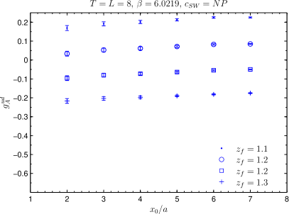
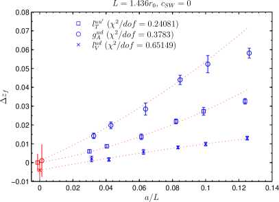
Figure 1: Left panel: varying $z_{f}$ does not change the slope of $g_{\rm A}^{ud}(x_{0})$, which is proportional to $m_{\mathrm{PCAC}}$. Right panel: different tuning conditions for $z_{f}$ yield O($a$) differences.

4.1 Tuning of $z_{f}$, boundary conditions

The tuning of $z_{f}$ can be performed by requiring any $\gamma_{5}\tau^{1}$-odd quantity to vanish [9]. Examples for such quantities are $g_{\rm P}^{uu^{\prime}}(x_{0})$, or $g_{\rm A}^{ud}(x_{0})$. Fortunately, the tuning of the parameters $m_{0}$ and $z_{f}$ is straightforward, as the respective tuning conditions are almost independent of each other (cf. also [16]). Given the critical value $m_{\rm cr}$ of $m_{0}$, we have also checked that the differences $\Delta z_{f}$ between $z_{f}$ values obtained from different conditions vanish with a rate $\propto a$, as expected (cf. fig. 1). Given $z_{f}(g_{0})$ one then expects that the boundary conditions (1) are correctly implemented up to cutoff effects. To test this hypothesis we have reverted the projectors $\tilde{Q}_{\pm}\rightarrow\tilde{Q}_{\mp}$ in the boundary sources and indicate this change by a subscript ”$-$” to the correlation functions. In the left panel of fig. 2 one indeed observes that the effect is very small and decreases towards zero. The corresponding result for the standard SF is very similar and given in the right panel of fig. 2.

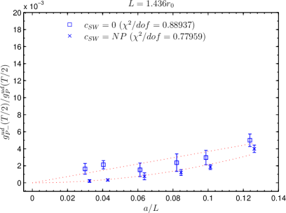
Figure 2: Check of boundary conditions, cf. main text for an explanation.

4.2 Universality relations

The universality relations (11),(12) are expected to hold between renormalized correlation functions. For instance one should then find that the ratios

$$\left[g_{\rm A}^{uu^{\prime}}(T/2)/\sqrt{g_{1}})\right]\times\left[f_{\rm A}(T/2)/\sqrt{f_{1}}\right]^{-1},\qquad\left[g_{\rm P}^{ud}(T/2)/\sqrt{g_{1}})\right]\times\left[f_{\rm P}(T/2)/\sqrt{f_{1}}\right]^{-1},$$ (13)

approach unity in the continuum limit. As seen in fig. 3, this is well satisfied within errors.

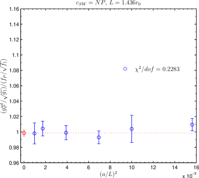
Figure 3: Universality checks: we consider ratios which should approach unity in the continuum limit.

4.3 Automatic O($a$) improvement

Automatic bulk O($a$) improvement relies on the fact that the bulk O($a$) effects are located in $\gamma_{5}\tau^{1}$-odd correlation functions. By projecting on the $\gamma_{5}\tau^{1}$-even correlators one thus gets rid of the bulk O($a$) effects. Here we study the $\gamma_{5}\tau^{1}$-odd correlators and verify that these vanish in the continuum limit with a rate $\propto a$, as can be seen in fig. 4 for $l_{\rm T}^{uu^{\prime}}(T/2)$. The corresponding standard SF correlator is also shown and vanishes exactly after gauge average, as expected due to parity and flavour symmetries. Another example is the counterterm contribution $\propto c_{\rm A}(a/L)$ needed to improve correlation functions of the axial current [6]. The result in this case is shown in the right panel of fig. 4. While the continuum limit vanishes in the chirally rotated SF, it is finite in the standard SF. Hence its contribution to axial current correlators is of O($a^{2}$) and O($a$), respectively, thereby confirming the expectation from automatic O($a$) improvement.

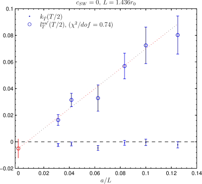
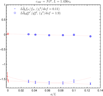
Figure 4: Check of automatic O($a$) improvement, cf. main text for details.

4.4 Determination of $Z_{\rm A,V}$

Having checked universality we may turn the tables and use universality to determine a number of finite renormalization constants which are usually determined from chiral Ward identities. For instance, the continuum relations (11) imply that $Z_{\rm A,V}$ can be determined by the ratios,

$$Z_{\rm A}=ig^{ud}_{\bar{\rm V}}(T/2)/g_{\rm A}^{uu^{\prime}}(T/2),\qquad Z_{\rm V}=g^{ud}_{\bar{\rm V}}(T/2)/g_{\rm V}^{ud}(T/2),$$ (14)

where $\bar{V}_{\mu}$ denotes the conserved vector current. The results in fig. 5 are subject to an O($a^{2}$) uncertainty, which perfectly explains the discrepancy with the Ward identity results of ref. [17].

5 Conclusions

We have presented a successful implementation of the chirally rotated Schödinger functional. Universality could be confirmed by comparing with standard SF correlation functions and automatic O($a$) improvement has been verified. In the future, we expect this framework to yield better controlled continuum extrapolations for step-scaling functions. Furthermore it provides new methods to determine finite renormalizaiton constants and O($a$) improvement coefficients for gauge theories with Wilson-type fermions.

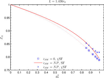
Figure 5: Determination of current normalization constants. The solid line is the fit function from the Ward identity determination [17] with non-perturbatively tuned $c_{\rm sw}$ [11].

Acknowledgments

The numerical simulations have been performed at the Trinity Centre for High Performance Computing and the Irish Centre for High End Computing. We thank both institutions for their support. B.L. has been partially supported by Science Foundation Ireland under grant 06/RFP/PHY061. Funding by the EU unter Grant Agreement number PITN-GA-2009-238353 (ITN STRONGnet) is gratefully acknowledged.

References

- [1] M. Lüscher, R. Narayanan, P. Weisz and U. Wolff, Nucl. Phys. B 384 (1992) 168.
- [2] S. Sint, Nucl. Phys. B 421 (1994) 135.
- [3] S. Sint, Nucl. Phys. B 451 (1995) 416.
- [4] K. Jansen et al., Phys. Lett. B 372 (1996) 275.
- [5] B. Sheikholeslami and R. Wohlert, Nucl. Phys. B 259 (1985) 572.
- [6] M. Lüscher, S. Sint, R. Sommer and P. Weisz, Nucl. Phys. B 478 (1996) 365.
- [7] R. Frezzotti and G. C. Rossi, JHEP 0408 (2004) 007.
- [8] S. Sint, PoS LAT2005 (2006) 235.
- [9] S. Sint, arXiv:1008.4857 [hep-lat].
- [10] S. Sint and P. Weisz, Nucl. Phys. B 502 (1997) 251.
- [11] M. Lüscher, S. Sint, R. Sommer, P. Weisz and U. Wolff, Nucl. Phys. B 491 (1997) 323.
- [12] R. Sommer, Nucl. Phys. B 411 (1994) 839.
- [13] S. Necco and R. Sommer, Nucl. Phys. B 622 (2002) 328.
- [14] M. Guagnelli, R. Petronzio and N. Tantalo, Phys. Lett. B 548 (2002) 58.
- [15] M. Lüscher, Comput. Phys. Commun. 165 (2005) 199; http://luscher.web.cern.ch/luscher/DD-HMC/index.html.
- [16] J. G. Lopez, K. Jansen, D. B. Renner and A. Shindler, PoS LAT2009 (2009) 199.
- [17] M. Lüscher, S. Sint, R. Sommer and H. Wittig, Nucl. Phys. B 491 (1997) 344.