Event-based simulation of light propagation in lossless dielectric media

Abstract

We describe an event-based approach to simulate the propagation of an electromagnetic plane wave through dielectric media. The basic building block is a deterministic learning machine that is able to simulate a plane interface. We show that a network of two of such machines can simulate the propagation of light through a plane parallel plate. With properly chosen parameters this setup can be used as a beam splitter. The modularity of the simulation method is illustrated by constructing a Mach-Zehnder interferometer from plane parallel plates, the whole system reproducing the results of wave theory. A generalization of the event-based model of the plane parallel plate is also used to simulate a periodically stratified medium.

1 Introduction

Maxwell’s theory of electrodynamics forms the basis of the understanding of the properties of light [1]. The Maxwell equations describe the evolution of electromagnetic fields in space and time [1]. They apply to a wide range of different physical situations and play an important role in a large number of engineering applications. Maxwell’s theory describes physical phenomena in terms of waves of electromagnetic radiation, yielding a simple explanation for the observation of interference phenomena. For many applications, computer simulation methods are required to solve Maxwell’s equations, the work horse being the finite-difference time-domain (FDTD) method [2].

In this paper, we present an alternative to the FDTD method. In contrast to a wave-based description, our approach uses particles (photons) that interact with matter. The simulation proceeds event-by-event, that is particle-by-particle. There is no direct communication/interaction between different particles: Indirect communication takes place via the interaction with matter, an interaction that is modeled by means of a deterministic learning machine (DLM) [3, 4, 5]. As we show in the paper, our approach is modular and yields the same stationary-state results as those obtained from Maxwell’s theory.

In section 2, we introduce the simulation approach and explain how it can be used to describe the reflection properties of a single interface, including interference effects (section 3). The modularity of our approach is illustrated by combining two or more DLMs to describe a homogeneous dielectric film (section 4) and a multilayer (section 5). Finally, we show that the basic building blocks can be re-used without modification to simulate more complex optical devices such as a Mach-Zehnder interferometer (MZI) (section 6).

2 Reflection and refraction at an interface

2.1 Wave theory

Figure 1: Reflection and refraction of light at a plane interface in the plane of incidence. The angle of refraction $\theta_{t}$ is determined by the angle of incidence $\theta_{i}$ and the refractive indices of both media $n_{1}$ and $n_{2}$ (Eq. 2). The angle of reflection $\theta_{r}$ is equal to the angle of incidence $\theta_{i}$.

In classical electrodynamics the laws of reflection and refraction are derived from Maxwell’s theory. In case of a plane wave incident on an interface between two homogeneous isotropic media with different optical properties, there is in general a transmitted wave and a reflected wave. The angle of incidence and the refractive indices of both media determine the direction of the transmitted and reflected part. Figure 1 shows a schematic picture in the plane of incidence. The relation between the angle of the incident ray $\theta_{i}$ and that of the reflected ray $\theta_{r}$ is determined by the law of reflection,

$$\theta_{r}=\theta_{i}.$$ (1)

The direction of the transmitted wave is determined by the law of refraction,

$$\frac{\sin\theta_{i}}{\sin\theta_{t}}=\frac{n_{2}}{n_{1}},$$ (2)

where $\theta_{t}$ is the angle of the transmitted ray, $n_{1}$ is the refractive index of the first and $n_{2}$ is that of the second medium (see Fig. 1).

For lossless, perfectly transparent media, the wave amplitudes are given by the Fresnel formulae [1]:

$$T_{\parallel} = \frac{2n_{1}\cos\theta_{i}}{n_{2}\cos\theta_{i}+n_{1}\cos\theta_{t}}A_{\parallel},$$ (3)

$$T_{\perp} = \frac{2n_{1}\cos\theta_{i}}{n_{1}\cos\theta_{i}+n_{2}\cos\theta_{t}}A_{\perp},$$ (4)

$$R_{\parallel} = \frac{n_{2}\cos\theta_{i}-n_{1}\cos\theta_{t}}{n_{2}\cos\theta_{i}+n_{1}\cos\theta_{t}}A_{\parallel},$$ (5)

$$R_{\perp} = \frac{n_{1}\cos\theta_{i}-n_{1}\cos\theta_{t}}{n_{1}\cos\theta_{i}+n_{2}\cos\theta_{t}}A_{\perp}.$$ (6)

The components of the electric field vector of the incident electromagnetic field parallel and perpendicular to the plane of incidence are denoted by $A_{\parallel}$ and $A_{\perp}$, respectively. $T_{\parallel}$ and $T_{\perp}$ are the amplitudes of the transmitted wave and $R_{\parallel}$ and $R_{\perp}$ are the amplitudes of the reflected wave.

The reflectivity $\mathcal{R}$ and the transmissivity $\mathcal{T}$ are given by

$$\mathcal{R}=\frac{|R|^{2}}{|A|^{2}},$$ (7)

and

$$\mathcal{T}=\frac{n_{2}}{n_{1}}\frac{\cos{\theta_{t}}}{\cos{\theta_{i}}}\frac{|T|^{2}}{|A|^{2}}.$$ (8)

Equations (7) and (8) are both valid for the parallel as well as for the perpendicular part and both components can be treated separately. Combining Eqs. (3) to (8) and simplifying the expressions gives [1]

$$\mathcal{R}_{\parallel} = \frac{\tan^{2}(\theta_{i}-\theta_{t})}{\tan^{2}(\theta_{i}+\theta_{t})},$$ (9)

$$\mathcal{R}_{\perp} = \frac{\sin^{2}(\theta_{i}-\theta_{t})}{\sin^{2}(\theta_{i}+\theta_{t})},$$ (10)

$$\mathcal{T}_{\parallel} = \frac{\sin 2\theta_{i}\sin 2\theta_{t}}{\sin^{2}(\theta_{i}+\theta_{t})\cos^{2}(\theta_{i}-\theta_{t})},$$ (11)

$$\mathcal{T}_{\perp} = \frac{\sin 2\theta_{i}\sin 2\theta_{t}}{\sin^{2}(\theta_{i}+\theta_{t})}.$$ (12)

2.2 Event-based simulation

We simulate the behavior of reflection and transmission at an interface by using an event-by-event, particle-only approach [3, 4, 5]. Clearly, in an event-based model of refraction and reflection at a dielectric, lossless interface, there can be no loss of particles: An incident particle must either bounce back from or pass through the interface. If such a model is to reproduce the results of Maxwell’s theory, the boundary conditions on the wave amplitudes in Maxwell’s theory must translate into a rule that determines how a particle bounces back or crosses the interface. In this section, we specify these rules.

We call an event the arrival of a single photon at the interface. This photon carries a message that can be interpreted as phase or time-of-flight information. As events occur one at a time only, there is no communication between individual photons, but the exchange and the processing of information takes place within the apparatus that describes the interface. An incoming photon will either be reflected or transmitted, depending on the state of the processing unit.

For later use, in addition to the input port and two output ports as depicted in Fig. 1, we add an additional input port that captures light incident from the opposite direction in such a way that the direction of a refracted outgoing particle coincides with the direction of a reflected particle of the opposite input port and vice versa (see Fig. 2).

Figure 2: Reflection and refraction of light at a plane interface in the plane of incidence. There are two input ports (0 and 1) and two output ports (0 and 1). The angles are chosen such that the direction of a refracted outgoing photon coincides with the direction of a reflected photon of the opposite input port and vice versa, allowing for interference to occur.

The processing unit in this case is a DLM [3, 4, 5] that takes messages from two input ports and sends out messages on either of two possible output ports depending on the internal state. The internal state is updated with each message that the DLM receives, i.e. it learns from the events that it processes.

The deterministic learning machine consists of three stages (see Fig. 3): The first stage receives an input from the n^th event, in this case the phase information $\phi$ of the photon and the angle of polarization $\varpi$, for practical reasons encoded as a four-dimensional vector $\mathbf{y}_{n}=((y_{n})_{0,\parallel},(y_{n})_{1,\parallel},(y_{n})_{0,\perp},(y_{n})_{1,\perp}),$ with $(y_{n})_{0,\parallel}=\cos(\phi)\cos(\varpi)$, $(y_{n})_{1,\parallel}=\sin(\phi)\cos(\varpi)$, $(y_{n})_{0,\perp}=\cos(\phi)\sin(\varpi)$, and $(y_{n})_{1,\perp}=\sin(\phi)\sin(\varpi)$. Upon arrival of a photon at one of its two input ports, the DLM stores the message in its internal register $\mathbf{Y}_{k}$ with $k=0$ or $k=1$ if the input was on port 0 or 1, respectively. There is also an internal vector $\mathbf{x}=(x_{0},x_{1})$ with $x_{i}\in[0,1],i=\{0,1\}$ and $x_{0}+x_{1}=1$. This vector is updated for each event received on port $k$ according to

$$(x_{n+1})_{i}=\alpha(x_{n})_{i}+(1-\alpha)\delta_{i,k},$$ (13)

where $0<\alpha<1$ is a parameter that determines the speed of learning. Since $(x_{n})_{0}+(x_{n})_{1}=1$ for all $n$, we can interpret $(x_{n})_{k}$ as (an estimate of) the frequency for the occurrence of an event on port $k$.

Figure 3: Schematic diagram of a DLM that performs an event-based simulation of a plane interface. There are two input ports and two output ports. The first stage (DLM) updates the internal registers $\mathbf{Y}_{0}$, $\mathbf{Y}_{1}$ and $\mathbf{x}$ according to the input $\mathbf{y}$. The second stage (T) processes the information stored in these registers according to a specific rule (Eq. (14)) and the third stage (O) prepares the outgoing message and sends it through one of the output ports.

The second stage processes the information stored in the registers $\mathbf{Y}_{0},\mathbf{Y}_{1}$ and $\mathbf{x}$ according to the rule

$$\mathbf{T}\left(\begin{array}[]{c}(Y_{0})_{0,\parallel}\sqrt{x_{0}}\\ (Y_{0})_{1,\parallel}\sqrt{x_{0}}\\ (Y_{1})_{0,\parallel}\sqrt{x_{1}}\\ (Y_{1})_{1,\parallel}\sqrt{x_{1}}\\ (Y_{0})_{0,\perp}\sqrt{x_{0}}\\ (Y_{0})_{1,\perp}\sqrt{x_{0}}\\ (Y_{1})_{0,\perp}\sqrt{x_{1}}\\ (Y_{1})_{1,\perp}\sqrt{x_{1}}\\ \end{array}\right)=\left(\begin{array}[]{c}r_{\parallel}(Y_{0})_{0,\parallel}\sqrt{x_{0}}+t_{\parallel}(Y_{1})_{0,\parallel}\sqrt{x_{1}}\\ r_{\parallel}(Y_{0})_{1,\parallel}\sqrt{x_{0}}+t_{\parallel}(Y_{1})_{1,\parallel}\sqrt{x_{1}}\\ t_{\parallel}(Y_{0})_{0,\parallel}\sqrt{x_{0}}-r_{\parallel}(Y_{1})_{0,\parallel}\sqrt{x_{1}}\\ t_{\parallel}(Y_{0})_{1,\parallel}\sqrt{x_{0}}-r_{\parallel}(Y_{1})_{1,\parallel}\sqrt{x_{1}}\\ r_{\perp}(Y_{0})_{0,\perp}\sqrt{x_{0}}+t_{\perp}(Y_{1})_{0,\perp}\sqrt{x_{1}}\\ r_{\perp}(Y_{0})_{1,\perp}\sqrt{x_{0}}+t_{\perp}(Y_{1})_{1,\perp}\sqrt{x_{1}}\\ t_{\perp}(Y_{0})_{0,\perp}\sqrt{x_{0}}-r_{\perp}(Y_{1})_{0,\perp}\sqrt{x_{1}}\\ t_{\perp}(Y_{0})_{1,\perp}\sqrt{x_{0}}-r_{\perp}(Y_{1})_{1,\perp}\sqrt{x_{1}}\\ \end{array}\right),$$ (14)

with

$$r_{\parallel} = \sqrt{\mathcal{R}_{\parallel}},$$ (15)

$$t_{\parallel} = \sqrt{\mathcal{T}_{\parallel}},$$ (16)

$$r_{\perp} = \sqrt{\mathcal{R}_{\perp}},$$ (17)

$$t_{\perp} = \sqrt{\mathcal{T}_{\perp}}.$$ (18)

Here we have omitted the event label $n$.

The third stage of the DLM prepares the messages

$$\mathbf{w}_{n}=\left(\begin{array}[]{c}t_{\parallel}(Y_{0})_{0,\parallel}\sqrt{x_{0}}-r_{\parallel}(Y_{1})_{0,\parallel}\sqrt{x_{1}}\\ t_{\parallel}(Y_{0})_{1,\parallel}\sqrt{x_{0}}-r_{\parallel}(Y_{1})_{1,\parallel}\sqrt{x_{1}}\\ t_{\perp}(Y_{0})_{0,\perp}\sqrt{x_{0}}-r_{\perp}(Y_{1})_{0,\perp}\sqrt{x_{1}}\\ t_{\perp}(Y_{0})_{1,\perp}\sqrt{x_{0}}-r_{\perp}(Y_{1})_{1,\perp}\sqrt{x_{1}}\\ \end{array}\right),$$ (19)

and

$$\mathbf{w}^{\prime}_{n}=\left(\begin{array}[]{c}r_{\parallel}(Y_{0})_{0,\parallel}\sqrt{x_{0}}+t_{\parallel}(Y_{1})_{0,\parallel}\sqrt{x_{1}}\\ r_{\parallel}(Y_{0})_{1,\parallel}\sqrt{x_{0}}+t_{\parallel}(Y_{1})_{1,\parallel}\sqrt{x_{1}}\\ r_{\perp}(Y_{0})_{0,\perp}\sqrt{x_{0}}+t_{\perp}(Y_{1})_{0,\perp}\sqrt{x_{1}}\\ r_{\perp}(Y_{0})_{1,\perp}\sqrt{x_{0}}+t_{\perp}(Y_{1})_{1,\perp}\sqrt{x_{1}}\\ \end{array}\right),$$ (20)

and generates a uniform random number $0<r<1$. If $\|\mathbf{w}_{n}\|>r$, the final stage sends $\mathbf{z}_{n}=\mathbf{w}_{n}/\|\mathbf{w}_{n}\|$ through port 0. Otherwise it sends $\mathbf{z}^{\prime}_{n}=\mathbf{w}^{\prime}_{n}/\|\mathbf{w}^{\prime}_{n}\|$ through port 1.

From the above construction of the DLM, it is clear that the connection between Maxwell’s wave description and the event-based, particle-like simulation model enters through Eqs. (15)-(18), where the expressions in the left-hand-sides of the latter are given by Eqs. (9)-(12).

2.3 Simulation results

As a first validation of the simulation model, we simulate a single interface with our event-based method. The initial values of the registers $\mathbf{Y}_{0},\mathbf{Y}_{1}$ and $\mathbf{x}$ are chosen randomly, but properly normalized. For each point in Fig. 4, 100000 events were simulated by sending messages on port 0 with a randomly chosen but fixed phase. The parameters were set to $\alpha=0.99$, $n_{1}=1$, and $n_{2}=1.52$. At the end we count, how many events we have detected on output port 0, i.e. the fraction of reflected particles. This normalized intensity corresponds to the reflectivity $\mathcal{R}$.

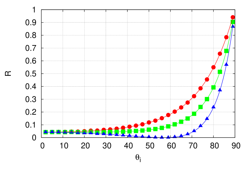
Figure 4: Reflectivity $\mathcal{R}$ of a plane interface between homogeneous dielectric media with refractive indices $n_{1}=1$ and $n_{2}=1.52$ as a function of the angle of incidence $\theta_{i}$. Triangles: Polarization angle $\varpi=0$; Squares: $\varpi=\pi/4$; Circles: $\varpi=\pi/2$. Each marker represents a simulation of 100000 events with $\alpha=0.99$. The simulation data are in very good agreement with the wave theoretical predictions (solid lines).

2.4 Discussion

We have shown that the reflectivity of a single interface can be simulated by our event-based approach. The simulation results are in excellent agreement with the theoretical predictions of Maxwell’s wave theory. Features such as the polarization dependence or reflection at the Brewster angle are faithfully reproduced. However, this good agreement does not show yet that our model correctly simulates interference phenomena. Such a demonstration is given in section 3.

3 Interference effects at an interface

In section 2, we dealt with the case of input on a single input port only. Here we consider the case where particles can arrive, one-by-one, on both sides of the interface, that is on both input ports.

3.1 Wave theory

According to Maxwell’s theory, if particles enter on input port 0 with a probability of $p_{0}$, carrying a phase $\phi_{0}$ and on input port 1 with probability $1-p_{0}$ and phase $\phi_{1}$ the amplitudes on the output ports are given by

$$\left(\begin{array}[]{c}b_{0}\\ b_{1}\end{array}\right)=\left(\begin{array}[]{cc}r_{\{\parallel,\perp\}}&t_{\{\parallel,\perp\}}\\ t_{\{\parallel,\perp\}}&-r_{\{\parallel,\perp\}}\end{array}\right)\left(\begin{array}[]{c}\sqrt{p_{0}}e^{i\phi_{0}}\\ \sqrt{1-p_{0}}e^{i\phi_{1}}\end{array}\right),$$ (21)

with $r_{\{\parallel,\perp\}}$ and $t_{\{\parallel,\perp\}}$ given by Eqs. (15) to (18). For S-polarization, i.e. the $\perp$-component ($\varpi=\pi/2$), the normalized intensity on output port 0 or the reflectivity $\mathcal{R}_{\perp}$ is given by

$$|b_{0,\perp}|^{2}=\frac{\sin^{2}(\theta_{i}-\theta_{t})}{\sin^{2}(\theta_{i}+\theta_{t})}p_{0}+\frac{\sin 2\theta_{i}\sin 2\theta_{t}}{\sin^{2}(\theta_{i}+\theta_{t})}(1-p_{0})\\ -2\frac{\sin(\theta_{i}-\theta_{t})\sqrt{\sin 2\theta_{i}\sin 2\theta_{t}}\cos(\phi_{0}-\phi_{1})}{\sin^{2}(\theta_{i}+\theta_{t})}\sqrt{p_{0}(1-p_{0})}.$$ (22)

For P-polarization ($\varpi=0$), the corresponding expression reads

$$|b_{0,\parallel}|^{2}=\frac{\tan^{2}(\theta_{i}-\theta_{t})}{\tan^{2}(\theta_{i}+\theta_{t})}p_{0}+\frac{\sin 2\theta_{i}\sin 2\theta_{t}}{\sin^{2}(\theta_{i}+\theta_{t})\cos^{2}(\theta_{i}-\theta_{t})}(1-p_{0})\\ +2\frac{\tan(\theta_{i}-\theta_{t})\sqrt{\sin 2\theta_{i}\sin 2\theta_{t}}\cos(\phi_{0}-\phi_{1})}{\tan(\theta_{i}+\theta_{t})\sin(\theta_{i}+\theta_{t})\cos(\theta_{i}-\theta_{t})}\sqrt{p_{0}(1-p_{0})}.$$ (23)

3.2 Simulation results

In Fig. 5 we compare the event-based simulation results to the wave theoretical predictions Eqs. (22) and (23). In these simulations, we send, one-by-one, photons with phase $\phi_{0}$ on port 0 with probability $p_{0}$ and photons with phase $\phi_{1}$ on port 1 with probability $1-p_{0}$. Of course, the results depend on the incident angle $\theta_{i}$.

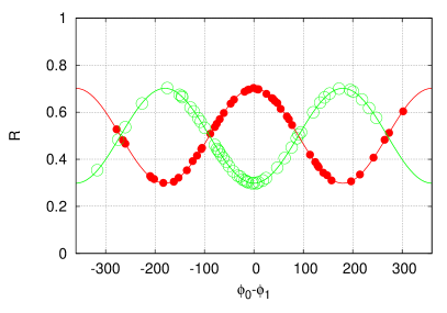
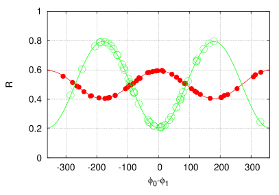
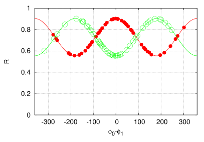
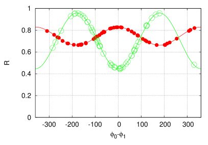
Figure 5: Single interface between a $n_{1}=1$ and a $n_{2}=1.52$ dielectric with input from both sides. Single photons arrive on port 0 with probability $p_{0}$, carrying a phase $\phi_{0}$ and on port 1 with probability $1-p_{0}$ and phase $\phi_{1}$. At any time there is at most one single photon in the system. Each marker represents a simulation of 100000 events with $\alpha=0.98$. The phase difference $\phi_{0}-\phi_{1}$ is generated from randomly chosen values of $\phi_{0}$ and $\phi_{1}$ (which are then fixed for 100000 events). Solid circles: Polarization angle $\varpi=0$; Open circles: $\varpi=\pi/2$. (a): $p_{0}=1/2$, $\theta_{i}=0$; (b): $p_{0}=1/2$, $\theta_{i}=\pi/4$; (c): $p_{0}=1/4$, $\theta_{i}=0$; (c): $p_{0}=1/4$, $\theta_{i}=\pi/4$. The simulation results are in excellent agreement with the theoretical expressions derived from wave theory (Eqs. (22) and (23)), shown here as solid lines.

3.3 Discussion

Our event-based simulation results are in excellent agreement with the wave theoretical description. For a single interface and a single input port there are no interference effects and the results are in agreement with wave theory, independent of the parameter $\alpha$. However, in the case of two input ports where interference can occur, the value of $\alpha$ is important: The wave theoretical predictions can only be reproduced by the event-based simulation if $\alpha$ is close to one [3, 4, 5].

4 Light propagation through a homogeneous dielectric film (plane-parallel plate)

A homogeneous dielectric film between two homogeneous media can be regarded as two plane parallel interfaces. Figure 6 shows a schematic picture of the system.

4.1 Wave theory

Figure 6: Homogeneous dielectric film built from two plane parallel interfaces. The film thickness is denoted by $h$. For a plate surrounded by air the refractive indices $n_{1}=n_{3}=1$ and $\theta_{1}=\theta_{3}$.

According to Maxwell’s theory, the reflectivity and transmissivity of the film are given by [1]

$$\mathcal{R}=\frac{r_{12}^{2}+r_{23}^{2}+2r_{12}r_{23}\cos 2\beta}{1+r_{12}^{2}r_{23}^{2}+2r_{12}r_{23}\cos 2\beta},$$ (24)

and

$$\mathcal{T}=\frac{n_{3}\cos\theta_{3}}{n_{1}\cos\theta_{1}}\frac{t_{12}^{2}t_{23}^{2}}{1+r_{12}^{2}r_{23}^{2}+2r_{12}r_{23}\cos 2\beta},$$ (25)

with

$$r_{12}=\frac{n_{1}\cos\theta_{1}-n_{2}\cos\theta_{2}}{n_{1}\cos\theta_{1}+n_{2}\cos\theta_{2}},$$ (26)

$$t_{12}=\frac{2n_{1}\cos\theta_{1}}{n_{1}\cos\theta_{1}+n_{2}\cos\theta_{2}},$$ (27)

for a S-polarized wave ($\varpi=\pi/2$) and

$$r_{12}=\frac{n_{2}\cos\theta_{1}-n_{1}\cos\theta_{2}}{n_{2}\cos\theta_{1}+n_{1}\cos\theta_{2}},$$ (28)

$$t_{12}=\frac{2n_{1}\cos\theta_{1}}{n_{2}\cos\theta_{1}+n_{1}\cos\theta_{2}},$$ (29)

for a P-polarized wave ($\varpi=0$), describing the process at the interface from medium 1 to medium 2 and analogous expressions for $r_{23}$ and $t_{23}$. The variable $\beta$ is determined by

$$\beta=\frac{2\pi}{\lambda_{0}}n_{2}h\cos\theta_{2},$$ (30)

with $\lambda_{0}$ being the wavelength of the incident wave and $h$ denoting the thickness of the film.

4.2 Event-based simulation

We simulate a homogeneous dielectric film by connecting two DLMs, one for each interface and each working as described in section 2. For each interface, we use the appropriate expressions for $r$ and $t$ as given by Eqs. (15)–(18) and Eqs. (9)–(12), that is we do not use the expressions from Maxwell’s theory for the film (Eqs. (24)–(30)). We recover the results of Maxwell’s theory by the event-based simulation without solving the wave equation for the film. This modularity allows us to re-use the DLM model of an interface for simulating films, multilayers etc.

We assume that the path of the particles is as depicted in Fig. 7. The incident particle is either reflected or refracted as it hits the first interface. In case of reflection it leaves the system on the front side of the film. If it is refracted, the particle refracted from the first interface acts as the incident particle of the second interface. While traveling from the first to the second interface it acquires a phase shift $\exp(i\Phi)$, with $\Phi=\beta$ (Eq. (30)), depending on the width of the film. Hitting the second interface there are again two options; either the particle is refracted and leaves the system on the back side of the film or it is reflected towards the first interface again, but this time entering the other input port after acquiring another phase shift on the way. Subsequently, a refraction leads to an exit on the front side of the film and on reflection the particle is sent back to the first input port of the second interface. This continues until eventually, the particle leaves on the front or the back side of the film.

Figure 7: A homogeneous dielectric film built from two plane parallel interfaces. Upon incidence on either of the two interfaces a photon can either be reflected or refracted. This can continue until it leaves on any side of the film. Due to the translational invariance when dealing with plane waves, corresponding translated paths can be regarded as superimposed.

The arrangement of the two DLMs is depicted in Fig. 8. This setup corresponds to the behavior described and shown in Fig. 7.

Figure 8: Arrangement of two DLMs simulating a homogeneous dielectric film. The output on port 0 of the second DLM is fed back into the input port 1 of the first machine. The symbol $\Phi$ denotes a phase shift that a message acquires when travelling that specific path.

4.3 Simulation results

With the setup of Fig. 8, we simulate the behavior of homogeneous dielectric films. The first analysis considers a plate of thickness $h=n_{2}\lambda_{0}/4$ (quarter-wave plate) under normal incidence for various values of refractive indices. The results for 100000 events and $\alpha=0.99$, together with the results of Maxwell’s theory, can be found in Fig. 9.

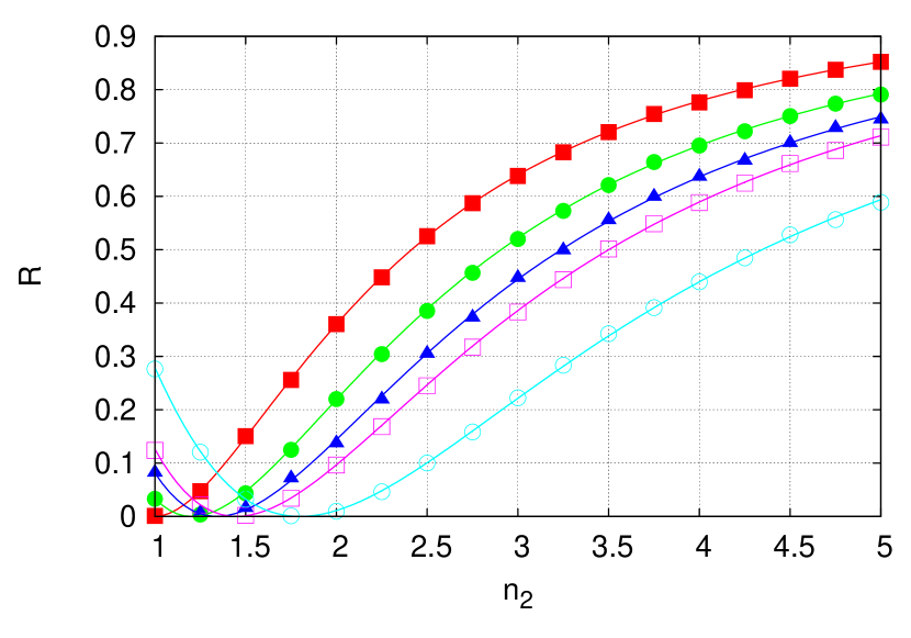
Figure 9: Simulation results of the reflectivity $\mathcal{R}$ of a quarter-wave plate, built from two plane parallel interfaces, for normal incidence and for various choices of refractive indices $n_{1}$, $n_{2}$ and $n_{3}$. Symbols represent simulation results with $\alpha=0.99$ and 100000 events per data point. Solid squares: $n_{1}=n_{3}=1$; Solid circles: $n_{1}=1$ and $n_{3}=1.45$; Triangles: $n_{1}=1$ and $n_{3}=1.8$; Open squares: $n_{1}=n_{3}=1.45$; Open circles: $n_{1}=n_{3}=1.8$; The solid lines are the wave theoretical predictions (Eq. (24)).

The values of the reflectivity predicted by wave theory (Eq. 24) are reproduced with high precision by the event-based simulation. Figure 10 shows the reflectivity under normal incidence of various plates surrounded by air ($n_{1}=n_{3}=1$) depending on the thickness of the plate.

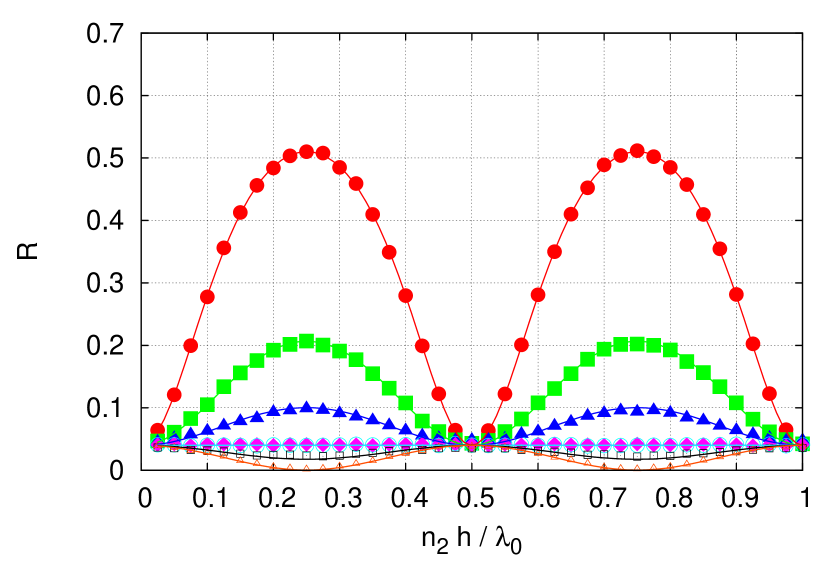
Figure 10: Simulation results of the reflectivity $\mathcal{R}$ of a homogeneous dielectric film for normal incidence ($\theta_{i}=0$) in air ($n_{1}=n_{3}=1$) as a function of its thickness $h$ for various values of $n_{2}$. Solid circles: $n_{2}=3$; Solid squares: $n_{2}=2$; Triangles: $n_{2}=1.7$; Open circles: $n_{2}=1$; Diamonds: $n_{2}=1.5$; Open squares: $n_{2}=1.4$; Open triangles: $n_{2}=1.2$. The parameter $\alpha=0.99$ and 100000 events were processed for each set of parameters. The simulation results (markers) are in very good agreement with the wave theoretical expressions (solid lines, Eq. (24)).

Again, the agreement with wave theory is very good. The variation with the incident angle for different polarizations is shown in Fig. 11.

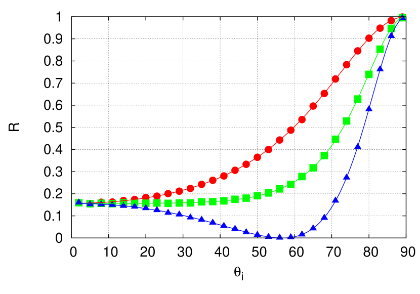
Figure 11: Simulation data of the reflectivity $\mathcal{R}$ of a quarter wave plate as a function of the angle of incidence $\theta_{i}$ for different polarizations $\varpi$. Triangles: Polarization angle $\varpi=0$; Squares: $\varpi=\pi/4$; Circles: $\varpi=\pi/2$. The parameter $\alpha=0.99$ and 100000 events were processed for each data point. The simulation results (markers) are in very good agreement with the wave theoretical expressions (solid lines, Eq. (24))

The wave theoretical predictions are all reproduced by the event-based simulation, including features like zero reflectivity under the Brewster angle for P-polarized ($\varpi=0$) light .

4.4 Application: beam splitter

Having shown that the event-based model of the homogeneous dielectric film works as expected, we now illustrate the modularity of the simulation approach by building a 50/50-beam splitter. The setup is shown in Fig. 12.

Figure 12: Beam splitter built from two plane parallel interfaces. The incident angle is set to $45^{\circ}$, the width to $h=\lambda_{0}/4n_{2}$, i.e. to an optical path length of a quarter wave and the refractive index $n_{2}$ is set to $n_{2}=1.86$, so that we get a 50/50-beam splitter ($n_{1}=n_{3}=1$, $\varpi=\pi/2$). There are two input ports and two output ports. Due to the translational invariance of plane waves, parallel paths (indicated by dotted lines) can be matched. This is also true for paths emerging from multiple reflections within the plate (not shown here, compare Fig. 7).

The incident angles are fixed to $45^{\circ}$, the width $h$ of the plate is set to $h=\lambda_{0}/4n_{2}$ and the refractive index $n_{2}$ of the plate is set to $n_{2}=1.86$, such that we get a 50/50-beam splitter for $\varpi=\pi/2$ (see Eq. (24)).

The incident particles on both input ports hit the beam splitter such that the direction of the transmitted particle from one port coincides with the direction of the reflected particle from the other input port. Due to the translational invariance of plane waves, parallel paths can be overlayed, as in the case of the plane parallel plate.

Next, we consider an experiment where we send, one-by-one, particles carrying the phase information $\phi_{0}$ ($\phi_{1}$) to input port 0 (1). The probability for a message to arrive on port 0 is $p_{0}$ and with probability of $1-p_{0}$ a message arrives on port 1. According to wave theory, the amplitudes $b_{0}$ and $b_{1}$ on the output ports 0 and 1 are given by [1]

$$\left(\begin{array}[]{c}b_{0}\\ b_{1}\end{array}\right)=\left(\begin{array}[]{cc}t&r\\ r&t\end{array}\right)\left(\begin{array}[]{c}\sqrt{p_{0}}e^{i\phi_{0}}\\ \sqrt{1-p_{0}}e^{i\phi_{1}}\end{array}\right),$$ (31)

with $r$ and $t$ given by

$$r=\frac{r_{12}+r_{23}e^{2i\beta}}{1+r_{12}r_{23}e^{2i\beta}},$$ (32)

and

$$t=\frac{t_{12}t_{23}e^{i\beta}}{1+r_{12}r_{23}e^{2i\beta}}.$$ (33)

The definitions of $r_{12}$ and $t_{12}$ are given in Eqs. (26) and (27), $r_{23}$ and $t_{23}$ are defined analogously.

Depending on the phase difference $\phi_{0}-\phi_{1}$ the probability for a particle to exit on the output port 0 is given by

$$|b_{0}|^{2}=\frac{1}{2}+\sqrt{p_{0}(1-p_{0})}\sin(\phi_{0}-\phi_{1}).$$ (34)

We have run the single-event simulation with $\alpha=0.98$ and $N_{0}+N_{1}=100000$ events for each value of the phase difference, where $N_{0}$ and $N_{1}$ denote the number of events on the output port 0 and 1, respectively. We determined the normalized intensity $N_{0}/(N_{0}+N_{1})$ detected on output port 0. The results for various values of $p_{0}$ are shown in Fig. 13.

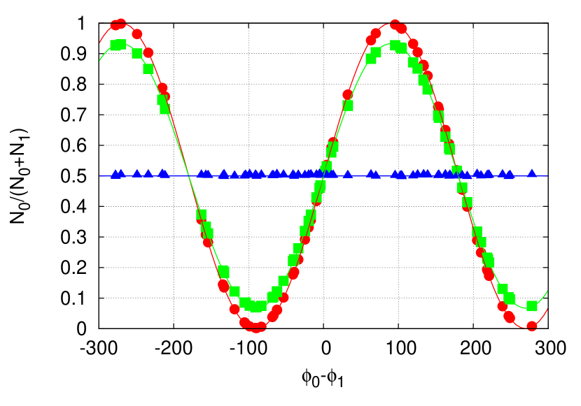
Figure 13: Simulation results for a 50/50-beam splitter built from two plane interfaces. The parameter $\alpha=0.98$ and 100000 events have been processed for each data point. The phases $\phi_{0}$ and $\phi_{1}$ were drawn from uniform random distributions. We measured the normalized intensity $N_{0}/(N_{0}+N_{1})$, with $N_{0}$ and $N_{1}$ being the number of events on the corresponding output port. Depending on the probability $p_{0}$ of an event entering on input port 0, we get different results which agree very well with the wave theoretical predictions (solid lines). Triangles: $p_{0}=1$; Circles: $p_{0}=0.5$; Squares: $p_{0}=0.25$.

The event-based simulation is in very good agreement with the behavior predicted by wave theory.

4.5 Discussion

We have shown that we can use an event-based simulation approach to describe the behavior of a homogeneous dielectric film. With the proper choice of parameters we can use this as a beam splitter. This beam splitter can be used as building block for optics experiments like the Mach-Zehnder interferometer (see section 6).

5 Light propagation through a periodic multilayer

5.1 Wave theory

A periodic multilayer consists of a succession of homogeneous layers of alternating refractive indices, $n_{2}$ and $n_{3}$, and thicknesses, $h_{2}$ and $h_{3}$, between two homogeneous media with refractive indices $n_{1}$ and $n_{4}$ (see Fig. 14).

Figure 14: Scheme of a periodic multilayer. It consists of a stack of layers with alternating refractive indices, $n_{2}$ and $n_{3}$, and thicknesses, $h_{2}$ and $h_{3}$ between two media with refractive indices $n_{1}$ and $n_{4}$. Drawn here are only three periods, but the number of periods can be chosen arbitrarily. It is also possible to end with the transition from $n_{2}$ to $n_{4}$ skipping the last layer with refractive index $n_{3}$.

For quarter wave layers ($n_{2}h_{2}=n_{3}h_{3}=\lambda_{0}/4$) at normal incidence the reflectivity for a total of $N$ interfaces is given by [1]

$$\mathcal{R}_{N}=\left(\frac{1-\left(\frac{n_{4}}{n_{1}}\right)\left(\frac{n_{2}}{n_{3}}\right)^{N-1}}{1+\left(\frac{n_{4}}{n_{1}}\right)\left(\frac{n_{2}}{n_{3}}\right)^{N-1}}\right)^{2},\quad\text{if $N$ is odd},$$ (35)

i.e., if the stack ends on $n_{3}\rightarrow n_{4}$, and

$$\mathcal{R}_{N}=\left(\frac{1-\left(\frac{n_{2}}{n_{1}}\right)\left(\frac{n_{2}}{n_{4}}\right)\left(\frac{n_{2}}{n_{3}}\right)^{N-2}}{1+\left(\frac{n_{2}}{n_{1}}\right)\left(\frac{n_{2}}{n_{4}}\right)\left(\frac{n_{2}}{n_{3}}\right)^{N-2}}\right)^{2},\quad\text{if $N$ is even},$$ (36)

i.e., if the stack ends on $n_{2}\rightarrow n_{4}$.

5.2 Event-based simulation

The method for simulating a plate consisting of two interfaces (section 4) can be generalized to the case of a multilayer. In this case we concatenate $N$ DLMs, each one simulating the behavior of a single interface. The schematic diagram of the DLM network is depicted in Fig. 15.

Figure 15: Network of DLMs for the simulation of a periodic multilayer. Here, only a single period ($n_{1}\rightarrow n_{2}\rightarrow n_{3}\rightarrow n_{4}$) with 3 interfaces is shown, but in principle it can be generalized to arbitrarily many periods. The first DLM on the left simulates a plane interface between media with refractive indices $n_{1}$ and $n_{2}$. The second DLM describes the transition from $n_{2}$ to $n_{3}$ and the third DLM simulates the interface between media with refractive indices $n_{3}$ and $n_{4}$. By inserting more DLMs before the rightmost one, it is possible to build any multilayer. For our simulation, we chose a periodic setup with alternating layers with reflective indices $n_{2}$ and $n_{3}$.

A message, that is sent into the network can propagate back and forth through any DLM, until eventually it leaves the network through port 0 of the first DLM or port 1 of the last DLM. This corresponds to multiple transmissions and reflections of a photon within the multilayer, until eventually it exits on the front or the back side.

5.3 Simulation results

We study the case of a periodic multilayer. The sequence of refractive indices along the stack is $n_{1}$, $n_{2}$, $n_{3}$, $n_{2}$, $n_{3}$, $\ldots$, $n_{2}$, ($n_{3}$), $n_{4}$ (figure 14). Figure 16 shows the reflectivity (normalized intensity on output port 0) depending on the number of interfaces.

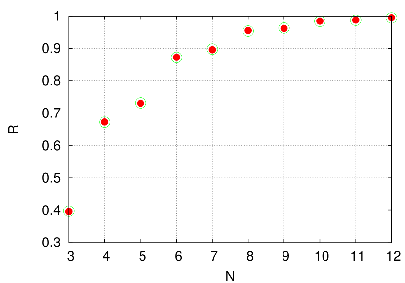
Figure 16: Reflectivity $\mathcal{R}$ of a periodic multilayer as a function of the number of interfaces $N$. Closed circles: Event-based simulation data. Open circles: Wave theory (Eqs. (35) and (36)). The parameters were chosen to resemble an experiment with quarter wave films of zinc sulphide and cryolite at normal incidence [1]: $n_{1}=1$, $n_{2}=2.3$, $n_{3}=1.35$, $n_{4}=1.52$, $n_{2}h_{2}=n_{3}h_{3}=\lambda_{0}/4$, $\theta_{i}=0$. The simulation was carried out with $\alpha=0.998$ and 1000000 events per data point. The results of our event-based approach agree very well with the predictions of wave theory.

Another analysis shows the reflectivity depending on the ratio $n_{2}/n_{3}$ (Fig. 17).

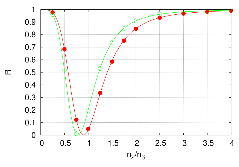
Figure 17: Reflectivity $\mathcal{R}$ of a periodic multilayer depending on the ratio $n_{2}/n_{3}$ of the refractive indices for $N=5$ (solid circles) and $N=6$ (open circles) interfaces. Data points are simulation results as obtained with $\alpha=0.99$ and 100000 events for each point. Solid lines are results derived from wave theory (Eqs. (35) and (36)). Model parameters are: $n_{1}=1$, $n_{2}=2$, $n_{4}=1.52$, $n_{2}h_{2}=n_{3}h_{3}=\lambda_{0}/4$, $\theta_{i}=0$, with $n_{3}$ varying. The event-by-event simulation gives the same results as the wave theoretical description (solid lines).

5.4 Discussion

We have shown that the approach introduced in section 2 can be generalized to multilayers by concatenating multiple DLMs. The basic building block is a DLM simulating a plane interface between two homogeneous dielectric media. A network of multiple DLMs can be used to form more complex structures. We studied the case of a periodic multilayer and found excellent agreement of the event-based simulation results with the wave theoretical description.

6 Event-based simulation of a Mach-Zehnder interferometer

6.1 Wave theory

The Mach-Zehnder interferometer is a device that is sensitive to relative phase shifts [1]. The schematic setup is depicted in Fig. 18.

Figure 18: Schematic setup of a Mach-Zehnder interferometer, consisting of two beam splitters and two devices that perform a specific phase shift. A photon is sent on one of the input ports and leaves the beam splitter on one of its output ports. Depending on which path of the interferometer a photon takes, its phase is changed by either $\psi_{0}$ or $\psi_{1}$. It then interacts with the second beam splitter and eventually, a photon is detected on one of the output ports of the interferometer. In the simulation we denote the photon numbers on each path with $N_{0}$, $N_{1}$, $N_{2}$, and $N_{3}$. The counts $N_{0}$ and $N_{1}$ give the number of particles that travel from the first to the second beamsplitter via one of the two pathways (but never via the two pathways simultaneously)

.

At any time, there is at most a single photon traveling through the system. After passing the first beam splitter the photon gets an additional phase shift depending on the path that it follows. It passes the second beam splitter and is detected on one of the output ports. According to wave theory the amplitudes of the photons $(b_{0},b_{1})$ in the output ports 0 ($N_{2}$) and 1 ($N_{3}$) are given by

$$\left(\begin{array}[]{c}b_{0}\\ b_{1}\end{array}\right)=\frac{1}{2}\left(\begin{array}[]{cc}1&i\\ i&1\end{array}\right)\left(\begin{array}[]{cc}e^{i\psi_{0}}&0\\ 0&e^{i\psi_{1}}\end{array}\right)\left(\begin{array}[]{cc}1&i\\ i&1\end{array}\right)\left(\begin{array}[]{c}a_{0}\\ a_{1}\end{array}\right),$$ (37)

with $(a_{0},a_{1})$ being the amplitudes in the input ports and $\psi_{0}$, $\psi_{1}$ describing the additional phase rotations in the specific arm of the interferometer.

For input on port 0 only, i.e. $(a_{0},a_{1})=(\cos\phi_{0}+i\sin\phi_{0},0)$, we get the probability distribution

$$|b_{0}|^{2}=\sin^{2}\left(\frac{\psi_{0}-\psi_{1}}{2}\right),\quad|b_{1}|^{2}=\cos^{2}\left(\frac{\psi_{0}-\psi_{1}}{2}\right).$$ (38)

6.2 Event-based simulation

We simulate a Mach-Zehnder interferometer with our event-based approach by using the same building blocks as shown in Fig. 18; we use two beam splitters, two phase shifters, one single-photon source (not shown) and two detectors (not shown). The beam splitters are built from more fundamental single interfaces as described in section 4.4. The communication between the components of the interferometer is mediated by single photons only. Each photon carries a message that is just its phase information.

The simulation results for input on a single port only, i.e. $(\cos\phi,\sin\phi)$ on port 0 and no input on port 1, are shown in Fig. 19. The phase $\phi$ is chosen randomly but fixed from an equal distribution in the range $[0,360^{\circ}]$. Each data point represents 100000 events $(N_{0}+N_{1}=N_{2}+N_{3}=100000)$ and $\alpha$ is set to $\alpha=0.98$. The angle of rotation $\psi_{0}$ is varying in steps of $10^{\circ}$ and the normalized intensities for the various ports are determined from the event-based simulation.

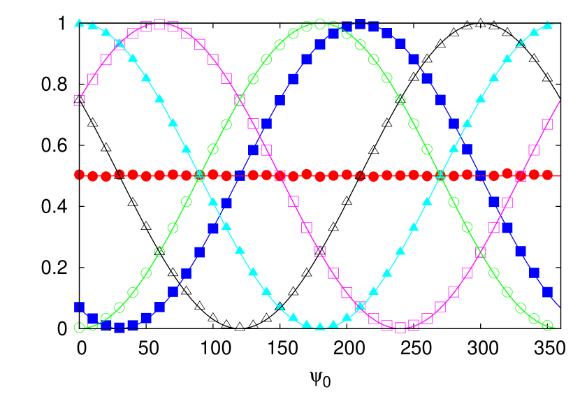
Figure 19: Normalized intensities in Mach-Zehnder interferometer (see Fig. 18) depending on the phase shift $\psi_{0}$ for various values of the phase shift $\psi_{1}$. The data points are simulation results using 100000 events and $\alpha=0.98$. Solid circles: $N_{0}/(N_{0}+N_{1})$ for $\psi_{1}=0$; Open circles: $N_{2}/(N_{2}+N_{3})$ for $\psi_{1}=0$; Solid squares: $N_{2}/(N_{2}+N_{3})$ for $\psi_{1}=30^{\circ}$; Open squares: $N_{2}/(N_{2}+N_{3})$ for $\psi_{1}=240^{\circ}$; Solid triangles: $N_{3}/(N_{2}+N_{3})$ for $\psi_{1}=0$; Open triangles: $N_{3}/(N_{2}+N_{3})$ for $\psi_{1}=300^{\circ}$; The solid lines are the predictions of wave theory.

The agreement between the event-based simulation and the wave theoretical description is very good if $\alpha$ is close to 1. This has been shown for event-based simulations with a DLM model that simulates a beam splitter as a whole [3, 4, 5], not as a collection of interfaces, as is done in the present work. Thus, we have shown that DLMs describing beam splitters can be built up from more fundamental building blocks, namely single interfaces, illustrating the modularity of our simulation method.

6.3 Discussion

Our event-based simulation of a MZI shows that this optics experiment can be simulated by building a network of a basic building block, the DLM-based machine that simulates an interfaces between two homogeneous media. The simulation results for the basic building block and the more complicated networks such as a plane parallel plate, a beam splitter, a periodic stratified medium, and a MZI are all in excellent agreement with the corresponding results of Maxwell’s theory, demonstrating that our event-based approach is modular. Crucial for the DLM-based simulation to yield the results of Maxwell’s theory is that the parameter $\alpha$ which controls the dynamics of the DLM is close to one [3, 4, 5].

7 Conclusion

We have shown that basic optical phenomena such as reflection, refraction and interference can be simulated by an event-based, particle-like approach. Our computational approach has the following features:

• It yields the stationary solution of the Maxwell equations by simulating particle trajectories only.

• Material objects are represented by DLM-based units placed on a boundary of these objects, which in practice involves some form of discretization. Apart from this discretization, all calculations are performed using Euclidean geometry.

• Unlike wave equation solvers, it does not suffer from artifacts due to the unavoidable termination of the simulation volume [2]: Particles that leave this volume can simply be removed from the simulation.

• Unlike wave equation solvers which may consume substantial computational resources (i.e. memory and CPU time) to simulate the propagation of waves in free space, it calculates the motion of the corresponding particles in free space at almost no computational cost.

• Modularity: Starting from the unit that simulates the behavior of a plane interface between two homogeneous media other optical components can be constructed by repeated use of the same unit.

We believe that the work presented in this paper may open a route to rigorously include the effects of interference in ray-tracing software. For this purpose, it is necessary to extend the DLM-based model for lossless dielectric materials to, say a Lorentz model for the response of material to the electromagnetic field [2]. This may be done by simple modifications of the DLM update rule, an extension that we leave for future research.

References

References

- [1] M. Born, E. Wolf, Principles of Optics, Pergamon, Oxford, 1964.
- [2] A. Taflove, S. Hagness, Computational Electrodynamics: The Finite-Difference Time-Domain Method, Artech House, Boston, 2005.
- [3] K. De Raedt, H. De Raedt, K. Michielsen, Deterministic event-based simulation of quantum interference, Comp. Phys. Comm. 171 (2005) 19 – 39.
- [4] H. De Raedt, K. De Raedt, K. Michielsen, New method to simulate quantum interference using deterministic processes and application to event-based simulation of quantum computation, J. Phys. Soc. Jpn. Suppl. 76 (2005) 16 – 25.
- [5] H. De Raedt, K. De Raedt, K. Michielsen, Event-based simulation of single-photon beam splitters and Mach-Zehnder interferometers, Europhys. Lett. 69 (2005) 861 – 867.