Fibred toric varieties in toric hyperkähler varieties

Abstract.

We introduce the fibred toric varieties as equivariant $\mathbb{C}P^{r}$ bundles over lower dimensional toric varieties. An equivalent characterization is that the natural morphisms on them degenerate to bundle projections in the context of variation of toric varieties as GIT quotients. Our main observation is that these fibred toric varieties also arise naturally in the variation of hyperkähler varieties, namely, the fibred toric varieties are contained in the exceptional sets of the hyperkähler natural morphisms and the Mukai flops.

1. Introduction

Toric varieties are defined by the combinatorial data of the fan (cf. [Ful93] or [Oda88]) as algebraic varieties, also studied by Delzant ([Del88]) in symplectic quotient perspective, associated to polytopes by moment maps, and later Guillemin ([Gui94b]) proved their canonical symplectic forms are in effect Kähler. More over, the symplectic quotient has natural connection with the Geometric Invariant Theory(short as GIT, cf. [MFK94]).

Toric hyperkähler varieties are quaternion analogue of toric varieties, which can be obtained as symplectic quotient of level set of the holomorphic moment map. Using symplectic quotient technique, in [BD00], Bielawski and Dancer studied their moment maps, cores, cohomologies, etc. While Hausel and Sturmfels study the toric hyperkähler varieties from a more algebraic view point([HS02]).

Choosing different level sets of moment map, conducting the symplectic quotient, we get different toric varieties and toric hyperkähler varieties respectively. It is natural to ask how the varieties change as the values of moment maps change. The symplectic quotient amounts to GIT quotient if we take the value of moment map to be the linearization of the torus action on line bundle. Thus the dependence of symplectic quotient to the level set is transferred to the dependence of GIT quotient to the linearization, which had been studied abstractly by Thaddeus in [Tha96], Dolgachev and Hu in [DH98]. In the toric case, there is some related discussion on toric varieties in [CLS11], and Konno studied the variation of toric hyperkähler varieties: the natural morphisms and Mukai flops, getting more special results(cf. [Kon03],[Kon08]).

In this article, we give the definition of fibred toric variety, then show that it takes key position in both variations of toric varieties and toric hyperkäher varieties. The advantages in toric category are the computation can be made directly based on the definitions of GIT, and more importantly, the variation of GIT quotients can be visualized by the variation of the hyperplane arrangements which can offer us more geometric information. In detail, this article is organized as follows. In section 2, after the symplectic quotient construction of toric variety, where the toric variety can be determined either by $\alpha$ a value of moment map or $\mathcal{A}$ a hyperplane arrangement, the fibred toric variety is defined.

Definition 1.1.

We call a $(r+s)$-dimensional toric variety $X$ fibred toric variety, if it is a $\mathbb{C}P^{r}$ bundle over $s$-dimensional toric variety $X_{1}$, and the bundle projection map is $T^{s}_{\mathbb{C}}$ equivariant, i.e. the $T^{s}_{\mathbb{C}}$ torus action of $X_{1}$ lifted to $X$ as a subgroup of $T^{r+s}_{\mathbb{C}}$, making the following diagram commutes.

$$\begin{CD}X@>{\rm T^{s}_{\mathbb{C}}\subset T^{r+s}_{\mathbb{C}}}>{}>X\\ @V{}V{}V@V{}V{}V\\ X_{1}@>{\rm T^{s}_{\mathbb{C}}}>{}>X_{1}\\ \end{CD}$$

In the end of section, the regularity of the toric variety $X(\alpha)$ is precisely described by the chamber structure on $\mathfrak{m}^{*}_{+}$.

In section 3, we establish the GIT quotient construction of toric variety, which is equivalent to the former symplectic one. Then we focus on the variation of toric varieties as GIT quotient where the following theorem is proven. Here $\alpha^{\pm}$ are two regular value in adjacent chambers, $\alpha_{1}$ is a singular lying on the generic position of the wall and $\pi^{\pm}$ are the natural morphisms form toric varieties $X(\alpha^{\pm})$ to $X(\alpha_{1})$.

Theorem 1.2.

(1) If we set $V_{1}=\{[z]\in X(\alpha_{1})|z\zeta=z,\ for\ \zeta\in G_{1}\}$, then $V_{1}$ is a toric variety.

(2) If we set $V^{+}=(\pi^{+})^{-1}(V_{1})$, $V^{-}=(\pi^{-})^{-1}(V_{1})$, then $\pi^{\pm}|_{V^{\pm}}:V^{\pm}\rightarrow V_{1}$ are fiber bundles whose fibers are biholomorphic to $\mathbb{C}P^{\#J_{1}^{\pm}-1}$, where $\#J_{1}^{+}$ $\#J_{1}^{-}$ are the numbers of elements in $J_{1}^{+}$ and $J_{1}^{-}$ respectively.

(3) Natural morphisms $\pi^{\pm}|_{X(\alpha^{\pm})\backslash V^{\pm}}:X(\alpha^{\pm})\backslash V^{\pm}\rightarrow X(\alpha_{1})\backslash V_{1}$ are both biholomorphic maps.

In the case $\alpha_{1}$ lies in a wall which is the boundary of $\mathfrak{m}^{*}_{+}$, $X(\alpha^{-})$ is empty, thus the natural morphism $\pi^{+}$ from $X(\alpha^{+})$ to $X(\alpha_{1})$ degenerates to a bundle projection with fiber a projective space. Hence $X(\alpha^{+})$ is a fibred toric variety. And it is showed that all fibred toric variety comes in this way.

Section 4 is parallel to section 2. Most properties of toric variety have their analogues in toric hyperkähler case. Additionally, we mainly review the result in [Pro08] and [BD00] concerning the extended core and core of toric hyperkähler variety, which establishes the deep connection between toric variety and toric hyperkähler variety.

Our discussion in section 5 on the variation of toric hyperkähler variety is highly influenced by Konno’s works. He described toric hyperkähler varieties as GIT quotient and studied the natural morphisms and Mukai flops of them, which take similar forms with the toric varieties.

Theorem 1.3.

[Kon03, Kon08]

(1) If we set $V_{1}=\{[z,w]\in Y(\alpha_{1},\beta)|(z,w)\zeta=(z,w)\ \text{for}\ \zeta\in G_{1}\}$, then $V_{1}$ is a toric hyperkähler variety.

(2) If we set $V^{\pm}=(\pi^{\pm})^{-1}(V_{1})$, then $\pi|_{V^{\pm}}:V^{\pm}\rightarrow V_{1}$ are fiber bundles whose fiber is biholomorphic to $\mathbb{C}P^{\#J_{1}-1}$. Moreover, the complex codimension of $V_{1}$ and $V^{\pm}$ in $Y(\alpha_{1},\beta)$ and $Y(\alpha^{\pm},\beta)$ are $2(\#J_{1}-1)$ and $\#J_{1}-1$ respectively, where $\#J_{1}$ is the number of elements in $J_{1}$.

(3) The natural morphism $\pi^{\pm}|_{Y(\alpha^{\pm},\beta)\backslash V^{\pm}}:Y(\alpha^{\pm},\beta)\backslash V^{\pm}\rightarrow Y(\alpha_{1},\beta)\backslash V_{1}$ are biholomorphic maps.

Take $\beta=0$, consider the natural morphism between $4n$ dimensional toric hyperähler varieties $\pi^{\pm}:Y(\alpha^{\pm},0)\rightarrow Y(\alpha_{1},0)$, it can be encoded as the variation of a smooth hyperplane arrangement $\mathcal{A}$ to a non-simplicial one $\mathcal{A}_{1}$ with $\mathcal{S}$ a lower dimensional arrangement as singular set. We have

Theorem 1.4.

Let $Z_{1}$ be the extended core of $V_{1}$ which is the toric varieties $X(\mathcal{S}_{\tilde{\epsilon}})$ intersecting together, Restrict $V^{\pm}$ these $\mathbb{C}P^{r}$ fiber bundles to $Z_{1}$, then $V^{\pm}|_{X(\mathcal{S}_{\tilde{\epsilon}})}$ the $\mathbb{C}P^{r}$ fiber bundles over each $X(\mathcal{S}_{\tilde{\epsilon}})$ are all fibred toric varieties of complex dimension $n$.

Acknowledgement: Both authors want to thank Prof. Bin Xu, Prof. Bailin Song, Dr. Yalong Shi and Dr. Yihuang Shen for valuable conversations and the second author want to thank his supervisor Prof. Yuxin Dong for constant encouragement.

2. Toric variety

Various descriptions of toric variety have their own advantages. We first consider the symplectic quotient, then shift to GIT quotient for the study of variation in next section.

2.1. Symplectic quotient(Kähler quotient)

The real torus $T^{d}=\{(\zeta_{1},\zeta_{2},\cdots,\zeta_{d})\in\mathbb{C}^{d},|\zeta_{i}|=1\}$ acts on $\mathbb{C}^{d}$ freely. Denote $M$ the $m$-dimensional connected subtorus of $T^{d}$ whose Lie algebra $\mathfrak{m}\subset\mathfrak{t}^{d}$ is generated by integer vectors(which is always taken to be primitive), then we have the following exact sequences

$$0\rightarrow\mathfrak{m}\xrightarrow{\iota}\mathfrak{t}^{d}\xrightarrow{\pi}\mathfrak{n}\rightarrow 0,$$

$$0\leftarrow{\mathfrak{m}}^{*}\xleftarrow{\iota^{*}}(\mathfrak{t}^{d})^{*}\xleftarrow{\pi^{*}}{\mathfrak{n}}^{*}\leftarrow 0,$$

where $\mathfrak{n}=\mathfrak{t}^{d}/\mathfrak{m}$ is the Lie algebra of the $n$-dimensional quotient torus $N=T^{d}/M$ and $m+n=d$. For simplicity, we omit the superscript $d$ over $\mathfrak{t}$ from now on.

Let $\{e_{i}\}_{i=1}^{d}$ be the standard basis of $\mathfrak{t}$, then $\pi(e_{i})=u_{i}$ are also primitive. Denote $\{e^{*}_{i}\}_{i=1}^{d}$ the dual basis of $\mathfrak{t}^{*}$ and $\{\theta_{i}\}_{i=1}^{m}$ some basis span $\mathfrak{m}$. The action of $M$ on $\mathbb{C}^{d}$ admits a moment map

$$\mu(z)=\frac{1}{2}\sum_{i=1}^{d}|z_{i}|^{2}\iota^{*}e^{*}_{i}.$$

For any $\alpha\in\mathfrak{m}^{*}$, the symplectic quotient $\mu^{-1}(\alpha)/M$ is a toric variety, denoted as $X(\alpha)$, inheriting Kähler metric from $\mathbb{C}^{d}$ on it’s smooth part(cf. [Gui94a]).

The quotient torus $N$ has a residue circle action on $X(\alpha)$ and gives rise to a moment map to $\mathfrak{n}^{*}$,

$$\bar{\mu}([z])=\frac{1}{2}\sum_{i=1}^{d}|z_{i}|^{2}e^{*}_{i}.$$

The image of this map is a convex polytope $\Delta$ called the Delzant polytope of $X(\alpha)$(cf. [Del88]). Conversely, any smooth compact toric variety $X$ of complex dimension $n$, with a Kähler metric invariant under some torus $N$ comes from Delzant’s construction. Unfortunately, this polytope does not recover all the data of the quotient construction, and the worse is that it does not cooperate well with the toric hyperkähler theory. We use the notion of hyperplane arrangement with orientation(cf. [Pro04]) to replace polytope. In detail, consider a set of rational oriented hyperplanes $\mathcal{A}=\{(H_{i},u_{i})\}_{i=1}^{d}$,

$$H_{i}=\{x\in\mathfrak{n}^{*}|\langle u_{i},x\rangle+\lambda_{i}=0\},$$

where $H_{i}$ is the hyperplane and $u_{i}$ is fixed primitive vector in $\mathfrak{n}_{\mathbb{Z}}$ specifying the orientation, called the normal of $H_{i}$. We define several subspaces related to these oriented hyperplanes,

$$H^{\geq 0}_{i}=\{x\in\mathfrak{n}^{*}|\langle u_{i},x\rangle+\lambda_{i}\geq 0\},$$

$$H^{\leq 0}_{i}=\{x\in\mathfrak{n}^{*}|\langle u_{i},x\rangle+\lambda_{i}\leq 0\}.$$

A ploytope is naturally associated to this arrangement,

$$\Delta=\bigcap^{d}_{i=1}H^{\geq 0}_{i},$$

which could be empty or unbounded.

The arrangement $\mathcal{A}$ will decide a toric variety the same as $\Delta$ does. Since $u_{i}$ define a map $\pi:\mathfrak{t}\rightarrow\mathfrak{n}$, where $\mathrm{Ker}\pi=\mathfrak{m}$, let $M$ be the Lie group corresponding to $\mathfrak{m}$ and set $\alpha=\sum\lambda_{i}\iota^{*}e_{i}^{*}$, then we call $\mu^{-1}(\alpha)/M$ the toric variety corresponding to $\mathcal{A}$ and $\lambda=(\lambda_{1},\cdots,\lambda_{d})$ a lift of $\alpha$. For fixed normal vectors, the hyperplane arrangements corresponding to two different lifts of same moment map value $\alpha$ only differ by a parallel transport, thus produce same toric variety(cf. [Pro04]). So we can abuse the notations $X(\alpha)$ and $X(\mathcal{A})$. Moreover, denote $\Theta$ the set of maps form $\{1,\dots,d\}$ to $\{-1,1\}$. For $\epsilon\in\Theta$, let $\mathcal{A}_{\epsilon}$ be the arrangement changing the normal of $H_{i}$ if $\epsilon(i)=-1$, and when $\epsilon(i)=1$ for all $i$, we abbreviate the subscript $\epsilon$ for simplicity. Notice that the toric variety $X(\mathcal{A}_{\epsilon})$ for various $\epsilon$ could be totally different.

Example 2.1 (see [BD00]).

We take $u_{1}=-f_{1}$, $u_{2}=u_{3}=f_{1}$ in $\mathfrak{n}^{1}$ where $f_{1}$ is the standard basis, and $\lambda_{1}=1$, $\lambda_{2}=-\frac{1}{2}$, $\lambda_{3}=0$. Hence $\mathfrak{m}$ is spanned by $\iota\theta_{1}=e_{1}+e_{2}$, $\iota\theta_{2}=e_{1}+e_{3}$, for short, $(1,1,0)$ and $(1,0,1)$. The toric variety is $\mathbb{C}P^{1}$. See Figure 1.

(a) the fan, where $u_{2}$, $u_{3}$ superposition

(b) the hyperplane arrangement and polytope which is represented by the bold line

Figure 1. the fan and hyperplane arrangement in Example 2.1

Example 2.2 (see [BD00] or [Pro04]).

Let $n=2$, $u_{1}=f_{1}$, $u_{2}=f_{2}$, $u_{3}=-f_{1}-f_{2}$, $u_{4}=-f_{2}$, and $\lambda_{1}=\lambda_{2}=\lambda_{3}=\lambda_{4}=1$. The toric variety is Hirzebruch surface $\mathbb{P}(\mathcal{O}\oplus\mathcal{O})$. See Figure 2.

(a) the fan

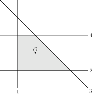
(b) the hyperplane arrangement and polytope which is represented by the shade area

Figure 2. the fan and hyperplane arrangement in Example 2.2

2.2. Definition of fibred toric variety

Now we state the definition of fibred toric variety.

Definition.

We call a $(r+s)$-dimensional toric variety $X$ fibred toric variety, if it is a $\mathbb{C}P^{r}$ bundle over $s$-dimensional toric variety $X_{1}$, and the bundle projection map is $T^{s}_{\mathbb{C}}$ equivariant, i.e. the $T^{s}_{\mathbb{C}}$ torus action of $X_{1}$ lifted to $X$ as a subgroup of $T^{r+s}_{\mathbb{C}}$, making the following diagram commutes.

$$\begin{CD}X@>{\rm T^{s}_{\mathbb{C}}\subset T^{r+s}_{\mathbb{C}}}>{}>X\\ @V{}V{}V@V{}V{}V\\ X_{1}@>{\rm T^{s}_{\mathbb{C}}}>{}>X_{1}\\ \end{CD}$$

The first nontrivial fibred toric variety is the Hirzebruch surface in Example 2.2, a $\mathbb{C}P^{1}$ bundle over $\mathbb{C}P^{1}$. And we will see this kind of toric varieties is very important in the variation of toric varieties and toric hyperkähler varieties.

2.3. Regularity

If the rational vectors $u_{i}$ is regular, i.e. every collection of $n$ linearly independent vectors $\{u_{i_{1}},\cdots,u_{i_{n}}\}$ span $\mathfrak{n}_{\mathbb{Z}}$ as a $\mathbb{Z}$-basis, then $\mathcal{A}$ is called regular. The arrangement $\mathcal{A}$ is called simplicial if every subset of $k$ hyperplanes with nonempty intersection intersects in codimension $k$. For a non-simplicial arrangement, all the points in the intersection of $k$ hyperplanes whose codimension is lower than $k$ are called singular set. $\mathcal{A}$ is smooth if it is both regular and simplicial.

Theorem 2.3 ([BD00],[Pro04]).

$X(\mathcal{A})$ is an orbifold, if and only if $\mathcal{A}$ is simplicial, and $X(\mathcal{A})$ is smooth if and only if $\mathcal{A}$ is smooth. When $\mathcal{A}$ is regular but non simplicial, it may attain Ablean quotient singularity.

From now on, $\mathcal{A}$ is always assumed regular to exclude the general orbifold singularities. The smoothness of hyperplane arrangement is closed related to the the moment map’s regularity. Let $\mathfrak{m}^{*}_{+}$ be the positive cone spanned by $\mathbb{R}_{\geq 0}\iota^{*}e_{i}^{*}$. Denote the isotropy subgroup of $M$ at $z\in\mathbb{C}^{d}$ by $M_{z}$, set $\Lambda=\{M_{z}|z\in\mathbb{C}^{d}\}$ and

$$\Lambda(k)=\{G\in\Lambda|\mathrm{dim}G=k\}\ \text{for}\quad k=0,\cdots,m.$$

Focusing on the set of one dimensional isotropy groups $\Lambda(1)=\{G_{s}\}_{s=1}^{l}$, we call the subspace in $\mathfrak{m}^{*}$ of codimension one

$$W_{s}=\{v^{*}\in\mathfrak{m}_{+}^{*}|\langle v^{*},\mathrm{Lie}G_{s}\rangle=0\}\subset\mathfrak{m}_{+}^{*}$$

a wall. Notice that the wall $W_{s}$ is spanned by $\{\mathbb{R}^{+}\iota^{*}e_{i}^{*}|\langle\iota^{*}e_{i}^{*},\mathrm{Lie}G_{s}\rangle=0\}$.

Proposition 2.4.

$$\mathfrak{m}^{*}_{+reg}=\mathfrak{m}^{*}_{+}\backslash\bigcup^{l}_{s=1}W_{s}$$

Proof.

Let $f:\mathbb{C}\rightarrow\mathbb{R}$ be a map defined by $f(a)=|a|^{2}$. We can easily observe that $a\in\mathbb{C}$ is a regular point of $f$ if and only if $a\neq 0$. Since $(\mathrm{d}\mu)(z)=\sum_{i=1}^{d}(\mathrm{d}f)_{z_{i}}\otimes\iota^{*}e_{i}^{*}\in\mathfrak{m}^{*}$, $(z)\in\mathbb{C}^{d}$ is a critical point of $\mu$ if and only if span $\{\iota^{*}e_{i}^{*}|z_{i}\neq 0\}\subsetneqq\mathfrak{m}^{*}$. This implies the proposition. ∎

There is an one to one correspondence between $\alpha$ and $\mathcal{A}$, if the fan $\{u_{i}\}$ is regular, then the smoothness of $\mathcal{A}$ and the regularity of moment map at $\alpha$ coincide. To see this, for fixed $\alpha\in\mathfrak{m}^{*}$, $\lambda$ is one of its lift, consider the equation

$$\alpha=\sum_{i=1}^{d}x_{i}\iota^{*}e_{i}^{*}.$$

Denoting the solution space as $\mathfrak{N}_{\alpha}$, a $n$-plane in $\mathbb{R}^{d}$, we have

Proposition 2.5.

Regarding the point $\lambda$ in $\mathfrak{N}_{\alpha}$ as the origin , projecting of $\mathfrak{N}_{\alpha}$ onto some standard $\mathbb{R}^{n}$, then we can identify $\pi_{\mathbb{R}^{n}}(\mathfrak{N}_{\alpha})$ with $\mathfrak{n}^{*}$, and the hyperplane arrangement $H_{i}$ is defined by $\pi_{\mathbb{R}^{n}}(\mathfrak{N}_{\alpha}\bigcap\{x_{i}=0\})$, where $\{x_{i}=0\}$ is the coordinate hyperplane in $\mathbb{R}^{d}$.

The proof can be found in [vCZ11]. Consequentially, $\mathcal{A}$ is non-simplicial means that there is a point $\lambda^{\prime}$ in $\mathfrak{N}_{\alpha}$ more than $n+1$ hyperplanes intersect in, i.e. more than $n+1$ coordinates $\lambda_{i}^{\prime}$ are zero. For $\lambda^{\prime}$ is also a new lift of $\alpha$, and $\alpha=\lambda_{i}^{\prime}\iota^{*}e_{i}^{*}$ at most involve $m-1$ terms, thus $\alpha$ must lie in a wall and vice versa.

Reader should notice that, even if $\alpha$ is singular or equivalently $\mathcal{A}$ is non-simplicial, the toric variety still has possibility to be smooth. For instance, $\lambda=(1,0,0)$, then $\alpha=\theta_{1}^{*}$ in Example 2.1, gives rise to $\mathbb{C}P^{1}$; or $\lambda=(1,1,1,2)$, then $\alpha=3(\theta_{1}^{*}+\theta_{2}^{*})$ in Example 2.2, gives rise to $\mathbb{C}P^{2}$.

The connected components of $\mathfrak{m}^{*}_{+reg}$ are called chambers. Within a chamber, the toric varieties are all biholomorphic. Therefore the only interesting variations are $\alpha$ moving into the wall or across the wall.

Example 2.6.

For the fan in Example 2.2, we have $\iota^{*}e_{1}^{*}=\iota^{*}e_{3}^{*}=\theta_{1}^{*}$, $\iota^{*}e_{2}^{*}=\theta_{1}^{*}+\theta_{2}^{*}$, $\iota^{*}e_{4}^{*}=\theta_{2}^{*}$. It’s chamber is drawn in Figure 3(a). If we change the fan to: $u_{1}=f_{1}$, $u_{2}=u_{4}=-f_{2}$, $u_{3}=-f_{1}-f_{2}$, i.e. change the direction of $u_{2}$, then we will have $\iota^{*}e_{1}^{*}=\iota^{*}e_{3}^{*}=\theta_{1}^{*}$, $\iota^{*}e_{2}^{*}=-\theta_{1}^{*}-\theta_{2}^{*}$, $\iota^{*}e_{4}^{*}=\theta_{2}^{*}$, as Figure 3(b).

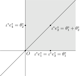
(a) the chamber of Example 2.2

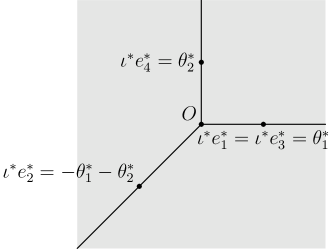
(b) the chamber of same arrangement but different orientation

Figure 3. two examples of chamber

3. Variation of toric variety

Since symplectic quotient is not suitable for the study of variation, a more intrinsic way to describe toric variety is necessary.

3.1. GIT quotient

Let us consider the GIT quotient of $\mathbb{C}^{d}$ by $M_{\mathbb{C}}$ with respect to the linearization induced by $\alpha\in\mathfrak{m}^{*}_{\mathbb{Z}}$. The element $\alpha$ induces the character $\chi_{\alpha}:M_{\mathbb{C}}\rightarrow\mathbb{C}^{\times}$ by $\chi_{\alpha}(\mathrm{Exp}(\rho\theta))=e^{\langle\alpha,\theta\rangle\rho}$, where $M_{\mathbb{C}}$ is the complexfication of $M$ and $\theta\in\mathfrak{m}$, $\rho\in\mathbb{C}$. Let $L^{\otimes m}=\mathbb{C}^{d}\times\mathbb{C}$ be the trivial holomorphic line bundle on which $M_{\mathbb{C}}$ acts as

$$((z),v)_{m}\zeta=((z)\zeta,v\chi_{\alpha}(\zeta)^{m})_{m}.$$

A point $(z)$ is $\alpha$-semi-stable if and only if there exists $m\in\mathbb{Z}_{>0}$ and a polynomial $f(p)$, where $p\in\mathbb{C}^{d}$, such that $f(p)$ viewed as a section of $L^{\otimes m}$ is invariant under the action, that is $f((p)\zeta)=f(p)\chi_{\alpha}(\zeta)^{m}$ for any $\zeta\in M_{\mathbb{C}}$, and additionally $f(z)\neq 0$. We denote the set of $\alpha$-semi-stable points in $\mathbb{C}^{d}$ by $(\mathbb{C}^{d})^{\alpha-ss}$, then there is a categorical quotient $\phi:(\mathbb{C}^{d})^{\alpha-ss}\rightarrow(\mathbb{C}^{d})^{\alpha-ss}//M_{\mathbb{C}}$, where $(\mathbb{C}^{d})^{\alpha-ss}//M_{\mathbb{C}}$ is the GIT quotient of $\mathbb{C}^{d}$ by $M_{\mathbb{C}}$ respect to $\alpha$(cf. [MFK94], and the readers are highly recommended to consult the lecture notes [Dol03] or [Tho06] if they prefer the variety rather than the abstract scheme setup). Sometimes $\mathbb{C}^{d}//_{\alpha}M_{\mathbb{C}}$ stands for this GIT quotient. We cite several basic properties of GIT quotient without proof.

Lemma 3.1.

For any point $p\in(\mathbb{C}^{d})^{\alpha-ss}//M_{\mathbb{C}}$, the fiber $\phi^{-1}(p)$ consists of finitely many $M_{\mathbb{C}}$-orbits. Moreover, each fiber contains the unique closed $M_{\mathbb{C}}$-orbits in $(\mathbb{C}^{d})^{\alpha-ss}$. Thus the categorical quotient $(\mathbb{C}^{d})^{\alpha-ss}//M_{\mathbb{C}}$ can be identified with the set of closed $M_{\mathbb{C}}$-orbits in $(\mathbb{C}^{d})^{\alpha-ss}$.

Unfortunately, the definition of stability respect to linearization is only effective when $\alpha\in\mathfrak{m}^{*}_{\mathbb{Z}}$, i.e. only corresponds to the algebraic toric variety with line bundle described by Newton ploytope with integer vertices. Following Konno’s method in hyperkähler case, it can be generalized to any complex manifold.

Definition 3.2.

Suppose that $\alpha\in\mathfrak{m}^{*}$,

(1) A point $z\in\mathbb{C}^{d}$ is $\alpha$-semi-stable if and only if

(3.1) $$\alpha\in\sum^{d}_{i=1}\mathbb{R}_{\geq 0}|z_{i}|^{2}\iota^{*}e_{i}^{*}.$$

(2) Suppose $z\in(\mathbb{C}^{d})^{\alpha-ss}$. Then the $M_{\mathbb{C}}$-orbit through $z$ is closed in $(\mathbb{C}^{d})^{\alpha-ss}$ if and only if

(3.2) $$\alpha\in\sum^{d}_{i=1}\mathbb{R}_{>0}|z_{i}|^{2}\iota^{*}e_{i}^{*}.$$

This definition of stability coincides the original GIT one when $\alpha\in\mathfrak{m}^{*}_{\mathbb{Z}}$. For convenience we give the proof of (1), and readers can find the essential proof of (2) in [Kon08]. Suppose $(z)\in(\mathbb{C}^{d})^{\alpha-ss}$. Then there exists $m\in\mathbb{Z}_{>0}$ and a polynomial $f(p_{1},\dots,p_{d})$ such that $f((p)\zeta)=f(p)\chi_{\alpha}(\zeta)^{m}$ and $f(z)\neq 0$. So we can select out a monomial $f_{0}(p)=\prod_{i=1}^{d}p_{i}^{a_{i}}$, where $a_{i}\in\mathbb{Z}_{>0}$, such that $f_{0}((p)\zeta)=f_{0}(p)\chi_{\alpha}(\zeta)^{m}$ and $f_{0}(z)\neq 0$. The second condition implies that $a_{i}=0\ \text{if}\ z_{i}=0$. Moreover, the first condition implies $m\alpha=\sum_{i=1}^{d}a_{i}\iota^{*}e_{i}^{*}$. To see this, let $\theta_{k}$ be the standard basis of $\mathfrak{m}$ and $\rho\in\mathbb{C}^{\times}$, we have $\chi(\mathrm{Exp}(\rho\theta_{k}))=e^{\rho\langle\alpha,\theta_{k}\rangle}$ and $(p)\mathrm{Exp}(\rho\theta_{k})=(p_{i}e^{\rho\langle\iota\theta_{k},e_{i}^{*}\rangle})=(p_{i}e^{\rho\langle\iota^{*}e_{i}^{*},\theta_{k}\rangle})$. Thus we proved Equation (3.1).

Proposition 3.3.

(1)If we fix $\alpha\in\mathfrak{m}^{*}$, then the natural map $\sigma:X(\alpha)\rightarrow(\mathbb{C}^{d})^{\alpha-ss}//M_{\mathbb{C}}$ is a homeomorphism(if $\alpha\notin\mathfrak{m}_{+}^{*}$, both sets are empty).

(2)If $\alpha\in\mathfrak{m}_{+reg}^{*}$, then every $M_{\mathbb{C}}$-orbit is closed in $(\mathbb{C}^{d})^{\alpha-ss}$. So the categorical quotient $(\mathbb{C}^{d})^{\alpha-ss}//M_{\mathbb{C}}$ is a geometric quotient $(\mathbb{C}^{d})^{\alpha-ss}/M_{\mathbb{C}}$.

Readers could consult [Kon08] for the proof. Thus the symplectic quotient $X(\alpha)$ can be identified with the GIT quotient $(\mathbb{C}^{d})^{\alpha-ss}//M_{\mathbb{C}}$ in both algebraic and holomorphic case. This principle was established in [KN78], [MFK94] in the algebraic case. The general holomorphic version is proved in [Nak99]. Variation of a toric variety with respect to fixed fan, means changing $\alpha$ the value of moment map in $\mathfrak{m}^{*}$(more precisely $\mathfrak{m}_{+}^{*}$), equals to altering the linearization of the GIT quotient. The variation of abstract GIT quotient had been studied thoroughly in [Tha96] and [DH98], but the toric variety case has its independent interest. This is because how $X(\alpha)$ varies can be read off from the variation of $\mathcal{A}$ directly. We will reprove some of their results in toric variety case, leading to more special consequence.

3.2. Natural morphism and flip

The phenomena of $\alpha$ moving from the interior of chamber into the wall is described by the so called natural morphism. Suppose $\alpha_{1}$ is in a generic position of the wall $W_{1}$ and $\alpha^{+}$, $\alpha^{-}$ lie in the chamber $\mathcal{C}^{+}$ and $\mathcal{C}^{-}$, s.t. $W_{1}\subset\overline{\mathcal{C}^{\pm}}$. By the stability condition Equation (3.1), $(\mathbb{C}^{d})^{\alpha^{\pm}-ss}\subset(\mathbb{C}^{d})^{\alpha_{1}-ss}$, inducing the natural morphisms between GIT quotients $\pi^{\pm}:X(\alpha^{\pm})\rightarrow X(\alpha_{1})$. The toric variety $X(\alpha_{1})$ may have singularity and these natural morphisms are kinds of “desingularization”. To see this, let $G_{1}$ be the 1-dimensional isotropy subgroup orthogonal to the wall $W_{1}$, and $\theta_{1}$ is a non-zero element in $\mathrm{Lie}G_{1}$ s.t. $\langle\theta_{1},\alpha_{1}\rangle>0$, set $J_{1}=\{i\in\{1,\cdots,d\}|\langle\iota^{*}e_{i}^{*},\theta_{1}\rangle\neq 0\}$, then $J_{1}$ divides into $J_{1}^{+}=\{i\in J_{1}\}|\langle\iota^{*}e_{i}^{*},\theta_{1}\rangle>0\}$ and $J_{1}^{+}=\{i\in J_{1}\}|\langle\iota^{*}e_{i}^{*},\theta_{1}\rangle<0\}$. Following Konno’s methods in hyperkähler case, we can prove Theorem 1.2.

The proof of Theorem 1.2: (1) Note that $W_{1}$ can be identified with the dual space of the Lie algebra $\mathfrak{m}_{1}$ of the quotient torus $M_{1}=M/G_{1}$. So $\alpha$ can be considered as a regular element of $\mathfrak{m}_{1}$. Then $V_{1}$ is a Kähler quotient of $\mathbb{C}^{\{1,...,d\}\backslash J_{1}}=\{(z)\in\mathbb{C}^{d}|z_{i}=0\ if\ i\in J_{1}\}$ by $M_{1}$.

(2) Choosing $\theta_{1}\in\mathrm{Lie}G_{1}$, by Equation (3.1) we know that $(\mathbb{C}^{d})^{\alpha^{+}-ss}$ is exactly the points in $(\mathbb{C}^{d})^{\alpha_{1}-ss}$ satisfying

(3.3) $$\text{there exists}\ i\in J_{1}^{+}\ \text{such that}\ z_{i}\neq 0.$$

For $\alpha^{+}$ is a regular value in $\mathfrak{m}^{*}$ and $\alpha_{1}$ a regular value in $\mathfrak{m}_{1}^{*}$, every orbit is closed respectively. Thus $V^{+}$ and $V_{1}$ are both geometric quotient, and $\pi^{+}|_{V^{+}}:V^{+}\rightarrow V_{1}$ can be interpreted as replacing $z_{i}$ with 0 in $[z]$ for any $i\in J_{1}^{+}$. Notice that if $(z)\in(\mathbb{C}^{d})^{\alpha^{+}-ss}$, then

(3.4) $$[z]\in V^{+}\ \text{is equivalent to}\ z_{i}=0\ \text{for all}\ i\in J^{-}_{1}.$$

Thus the fiber of $\pi^{+}|_{V^{+}}:V^{+}\rightarrow V_{1}$ is biholomorphic to $(\mathbb{C}^{\#J_{1}^{+}}\backslash\{0\})/G_{1\mathbb{C}}$, i.e. $\mathbb{C}P^{\#J_{1}^{+}-1}$. The case of $\pi^{-}$ is tautological.

(3) If $(z)\in(\mathbb{C}^{d})^{\alpha_{1}-ss}$, by Equation (3.3) and (3.4), then $[z]\in X(\alpha^{+})\backslash V^{+}$ equals to

$$\text{there exists}\ i\in J_{1}^{+}\ \text{such that}\ z_{i}\neq 0\ \text{and}\ j\in J_{1}^{-}\ \text{such that}\ z_{j}\neq 0.$$

This means nothing but

$$X(\alpha^{+})\backslash V^{+}=((\mathbb{C}^{d})^{\alpha^{+}-ss}\cap(\mathbb{C}^{d})^{\alpha^{-}-ss})/M_{\mathbb{C}},$$

and similarly

$$X(\alpha^{-})\backslash V^{-}=((\mathbb{C}^{d})^{\alpha^{-}-ss}\cap(\mathbb{C}^{d})^{\alpha^{+}-ss})/M_{\mathbb{C}}.$$

On the other hand, by Equation (3.2) in Definition 3.2, $(z)\in(\mathbb{C}^{d})^{\alpha^{+}-ss}\cap(\mathbb{C}^{d})^{\alpha^{-}-ss}$ implies the orbit $(z)M_{\mathbb{C}}$ is closed in $(\mathbb{C}^{d})^{\alpha_{1}-ss}$, finishing the proof. ∎

Recall there are two different kinds of walls in $\mathfrak{m}_{+}^{*}$: one is the boundary of $\mathfrak{m}^{*}_{+}$(may be boundaryless, for example Figure 3(b)), called boundary wall; the other lies in interior of $\mathfrak{m}^{*}_{+}$, called interior wall.

We focus on the boundary wall. Since $J_{1}^{-}$ is empty, $(\mathbb{C}^{d})^{\alpha^{-}-ss}$ is empty and $X(\alpha^{-})\backslash V^{-}$ is empty either. Thus by (3) in Theorem 1.2, $\pi^{+}$ degenerates to a bundle projection from $X(\alpha^{+})$ to $X(\alpha_{1})$ with fiber $\mathbb{C}P^{\#J_{1}-1}$. In effect, we have another way to see it directly. For $\alpha_{1}$ is on the boundary, by the closeness criterion Equation (3.2), the coefficients before $\iota^{*}e_{i}^{*},i\in J_{1}$ must all be zero, i.e. the only closed orbit in $(\mathbb{C}^{d})^{\alpha_{1}-ss}$ is the orbit through the point $\{z|z_{i}=0,\ for\ i\in J_{1}\}$. These points have a common isotropy group $G_{1}$, hence $X(\alpha_{1})$ can be viewed as a lower dimensional smooth toric variety corresponding to the group action of $M_{1}=M/G_{1}$ on $\mathbb{C}^{\{1,\dots,d\}\backslash J_{1}}$, and $\alpha_{1}\in(\mathfrak{m}^{*}_{1})_{reg}$. Thus we have $V_{1}=X(\alpha_{1})$ and $V^{+}=X(\alpha^{+})$, and $\pi^{+}:X(\alpha^{+})\rightarrow X(\alpha_{1})$ is a fiber bundle whose fiber is biholomorphic to $\mathbb{C}P^{\#J_{1}-1}$(the general case refers to the material in [Tha96], Corollary 1.13 and below).

In the interior wall case, since we know little about how $J_{1}$ divides into $J_{1}^{+}$ and $J_{1}^{-}$, the natural morphism related is much more complicated. This kind of natural morphism can not degenerate to bundle projection, and roughly speaking, is the generalization of blowup.

We are ready to investigate the variation of $\alpha$ cross the interior wall. The cross wall phenomena can be recovered by the two adjacent natural morphisms. For both natural morphisms $\pi^{+}$, $\pi^{-}$ can not degenerate, the exceptional sets $V^{+}$ and $V^{-}$ of $V_{1}$ are lower dimensional. Thus $\pi^{+}\circ(\pi^{-})^{-1}:X(\alpha^{+})\backslash V^{+}\rightarrow X(\alpha^{-})\backslash V^{-}$ is a biholomorphic map, and a birational map between $X(\alpha^{+})$ and $X(\alpha^{-})$, which is called flip by Thaddeus(cf. [Tha96]).

3.3. Relation with fibred toric variety

Based on above discussion, we know that for a given toric variety $X(\alpha)$, if $\alpha$ lies in the chamber next to the boundary wall, then $X(\alpha)$ is a fibred toric variety. In fact, we will show that all fibred toric varieties come from this kind construction.

We’d better give some configuration of the arrangement and the polytope of the variation of the fibred toric variety. By Proposition 2.5, up to biholomorphic equivalent class, the variation of $\alpha$ into the wall or cross the wall is equivalent to moving some hyperplane $H_{i}$, $i\in J_{1}$ in $\mathcal{A}$ into or cross singular set of $\mathcal{A}_{1}$. Thus fibred toric variety is characterized as the hyperplane $H_{i}$ will never cross any other vertex of its polytope $E$ before the volume of this polytope tends to zero, i.e. $E$ degenerates to a lower dimensional polytope. Based on this observation, we can give a configuration of the fibred polytope.

Proposition 3.4.

The polytope $E$ defines a fibred toric variety has form of a product: $E=\Delta(r)\times F$ where $\Delta(r)$ is the standard polytope defining $\mathbb{C}P^{r}$, and $F$ is a $s$-dimensional polytope.

Proof.

Let $H$ be the moving hyperplane, move $H$ to a non-simplicial arrangement, we denote the singular set as $F$. Restricting $F$ to $E$, it is a face of the polytope $E$, and itself a lower dimensional smooth polytope, still denoted as $F$. At the same time, the restriction of $H$ to $E$ is also a smooth polytope of dimension $n-1$, still denoted as $H$.

We can first assume that $E$ is bounded. Suppose $H$ has $q$ vertices, and $F$ has $p$ vertices $\{o_{i},i=1,\dots,p\}$. For $E$ is smooth, each vertex has $n$ edges. The proof divides into three steps as follows.

Step1, notice the following two facts: one is the each vertex $o_{i}$ in $F$ has $r$ edges come from $F$. Another is $H$ can smoothly shrink to $F$ without passing any other vertex, so all other $s$ edges of $o_{i}$ come from the vertices belong to $H$. This means $s$ vertices of $H$ will map to one vertex in $F$, i.e. $q=p\cdot s$. Thus the vertices of $H$ can be labeled as $\{a_{i}^{j}\},j=1,\dots,s$, divide into $p$ groups.

Step2, consider the edges between different groups, we claim that there are at most $r$ edges shed from one vertex in $H$ to the vertices in other groups. This is because that by the parallel moving, we know all the edges shed from one vertex $a_{1}^{j}$ in $H$ come from parallel moving the edges shed from $o_{1}$ in $F$, while there are only $r$ edges shed from $o_{1}$.

So there are at most $\frac{q\cdot r}{2}$ edges between different groups in $H$. Hence the sum of edges inside each groups are at least:

(3.5) $$\frac{q(n-1)}{2}-\frac{q\cdot r}{2}=\frac{q(s-1)}{2}=\frac{p\cdot s(s-1)}{2},$$

where $\frac{q(n-1)}{2}$ is number of total edges in the polytope $H$.

Step3, for in each individual group, there is at most $\frac{s(s-1)}{2}$ edges between $s$ points, by Equation (3.5), each vertex must have exactly $r$ edges joining other groups, and $s-1$ edges joining other $s-1$ point in its own group constituting a $\Delta(s-1)$.

In conclusion $H$ can be written as $\Delta(s-1)\times F$, then $E$ is of the form $\Delta(s)\times F$.

If $E$ is unbounded, firstly, we apply above argument to its bounded faces, combining the fact each radial in $H$ comes form the radial in $F$ by parallel moving, accomplish the proof. ∎

For a fibred toric variety $X$, we endow a fixed fiber $\mathbb{C}P^{r}$ the Fubini-Study metric, pull back the Fubini-Study metric to all the fibers by the $T^{s}_{\mathbb{C}}$ action. Then we give $X_{1}$ the $T^{s}$ invariant Kähler metric, and $X$ the horizontal part metric which makes the projection a Riemann submersion. For the projection is $T^{s}_{\mathbb{C}}$ equivariant, the Kähler metric on $X$ is $T^{r+s}$ equivariant. If we rescale the Fubini-Study metric by a number tends to zero, then $X$ will degenerate to $X_{1}$, while the $n$ dimensional moment polytope of $X$ degenerate to a $s$ dimensional moment polytope. This procedure reproduce the variation above. Thus all fibred toric varieties arise in this way.

4. Toric hyperkähler variety

A $4n$-dimensional manifold is hyperkähler if it possesses a Riemannian metric $g$ which is Kähler with respect to three complex structures $I_{1}$; $I_{2}$; $I_{3}$ satisfying the quaternionic relations $I_{1}I_{2}=-I_{2}I_{1}=I_{3}$ etc. To date the most powerful technique for constructing such manifolds is the hyperkähler quotient method of Hitchin, Karlhede, Lindstrom and Rocek([HKLR87]). We specialized on the class of hyperkähler quotients of flat quaternionic space $\mathbb{H}^{d}$ by subtori of $T^{d}$. The geometry of these spaces turns out to be closely connected with the theory of toric varieties.

4.1. Symplectic quotient(hyperkähler quotient)

Since $\mathbb{H}^{d}$ can be identified with $T^{*}\mathbb{C}^{d}\cong\mathbb{C}^{d}\times\mathbb{C}^{d}$, it has three complex structures $\{I_{1},I_{2},I_{3}\}$. The real torus $T^{d}=\{(\zeta_{1},\zeta_{2},\cdots,\zeta_{d})\in\mathbb{C}^{d},|\zeta_{i}|=1\}$ acts on $\mathbb{C}^{d}$ inducing a action on $T^{*}\mathbb{C}^{d}$ keeping the hyperkähler structure,

$$(z,w)\zeta=(z\zeta,w\zeta^{-1}).$$

The subtours $M$ acts on it admitting a hyperkähler moment map $\mu=(\mu_{\mathbb{R}},\mu_{\mathbb{C}}):\mathbb{H}^{d}\rightarrow\mathfrak{m}^{*}\times\mathfrak{m}^{*}_{\mathbb{C}}$, given by,

$$\mu_{\mathbb{R}}(z,w)=\frac{1}{2}\sum_{i=1}^{d}(|z_{i}|^{2}-|w_{i}|^{2})\iota^{*}e^{*}_{i},$$

$$\mu_{\mathbb{C}}(z,w)=\sum_{i=1}^{d}z_{i}w_{i}\iota^{*}e^{*}_{i}.$$

where the complex moment map $\mu_{\mathbb{C}}:\mathbb{H}^{d}\rightarrow\mathfrak{m}^{*}_{\mathbb{C}}$ is holomorphic with respect to $I_{1}$. Bielawski and Dancer introduced the definition of toric hyperkähler varieties, and generally speaking, they are not toric varieties.

Definition 4.1 ([BD00]).

A toric hyperkähler variety $Y(\alpha,\beta)$ is a hyperkähler quotient $\mu^{-1}(\alpha,\beta)/M$ for $(\alpha,\beta)\in\mathfrak{m}^{*}\times\mathfrak{m}^{*}_{\mathbb{C}}$.

The smooth part of $Y(\alpha,\beta)$ is a $4n$-dimensional hyperkähler manifold, whose hyperkähler structure is denoted by $(g,I_{1},I_{2},I_{3})$. The quotient torus $N=T/M$ acts on $Y(\alpha,\beta)$, preserving its hyperkähler structure. This residue circle action admits a hyperkähler moment map $\bar{\mu}=(\bar{\mu}_{\mathbb{R}},\bar{\mu}_{\mathbb{C}})$,

$$\bar{\mu}_{\mathbb{R}}([z,w])=\frac{1}{2}\sum_{i=1}^{d}(|z_{i}|^{2}-|w_{i}|^{2})e^{*}_{i},$$

$$\bar{\mu}_{\mathbb{C}}([z,w])=\sum_{i=1}^{d}z_{i}w_{i}e^{*}_{i}.$$

Differs from the toric case, the map $\bar{\mu}$ to $\mathfrak{n}^{*}\times\mathfrak{n}^{*}_{\mathbb{C}}$ is surjective, never with a bounded image.

Parallel with section 2, we use hyperplane arrangement encoding the quotient construction. For the moment map takes value in $\mathfrak{m}^{*}\times\mathfrak{m}^{*}_{\mathbb{C}}$, the lift of $(\alpha,\beta)$ is $(\lambda^{1},\lambda^{2},\lambda^{3})$, s.t.

$$\begin{cases}&\alpha=\sum\lambda_{i}^{1}\iota^{*}e_{i}^{*}\\ &\beta=\sum(\lambda_{i}^{2}+\sqrt{-1}\lambda_{i}^{3})\iota^{*}e_{i}^{*}\end{cases}$$

Then we can construct the arrangement of codimension 3 flats (affine subspaces) in $\mathbb{R}^{3n}$,

$$H_{i}=H_{i}^{1}\times H_{i}^{2}\times H_{i}^{3},$$

where

$$H_{i}^{h}=\{x\in\mathfrak{m}^{*}|\langle u_{i},x\rangle+\lambda_{i}^{h}=0\},\ (h=1,2,3,\ i=1,\dots,d)$$

a prior with orientation $u_{i}$. For simplicity, we still denote this arrangement of flats as $\mathcal{A}$. Vice versa, such a arrangement of $\mathcal{A}$ determines a hyperkähler quotient $Y(\alpha,\beta)$. Different from the toric variety, toric hyperkähler manifolds according to the a arrangement with different orientations will be biholomorphic to each other(cf. [vCZ11]).

Example 4.2.

Let $\beta=0$ and $\alpha$ corresponds to the arrangement in Example 2.1. The resulted toric hyperkähler variety is the desingulariztion of $\mathbb{C}^{2}/\mathbb{Z}_{3}$(cf. [HS02], section 10).

4.2. Regularity

Variation the hyperkähler structure on a toric hyperkähler variety means altering $(\alpha,\beta)$ in $\mathfrak{m}^{*}\times\mathfrak{m}^{*}_{\mathbb{C}}$, hence the regularity of $(\alpha,\beta)$ is a crucial premise.

The hyperkähler chamber structure can be defined on $\mathfrak{m}^{*}\times\mathfrak{m}^{*}_{\mathbb{C}}$ rather than the positive cone $\mathfrak{m}^{*}_{+}$ the same as the toric variety case, and the walls are entire hyperspaces. For simplicity, we still use the same notation. There is

Proposition 4.3 ([Kon08]).

(1) $(\mathfrak{m}^{*}\times\mathfrak{m}^{*}_{\mathbb{C}})_{reg}=\mathfrak{m}^{*}\times\mathfrak{m}^{*}_{\mathbb{C}}\backslash\bigcup^{l}_{s=1}W_{s}\otimes W_{s\mathbb{C}}$, where $W_{s\mathbb{C}}$ is the complexification of $W_{s}$.

(2) If $(\alpha,\beta)\in(\mathfrak{m}^{*}\times\mathfrak{m}^{*}_{\mathbb{C}})_{reg}$, then $X(\alpha,\beta)$ is a smooth manifold.

Similarly, we define the connected components of $(\mathfrak{m}^{*}\times\mathfrak{m}^{*}_{\mathbb{C}})_{reg}$ to be the chambers. Example 4.4 illustrates that although it has the same expression with the toric one, the underlining structure is different.

Example 4.4.

Take $\beta=0$, consider the toric hyperkähler varieties corresponding to the two arrangements in Example 2.6. We draw their real part chambers in $\mathfrak{m}^{*}$ in Figure 4.

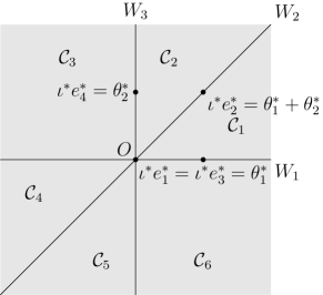
(a) the chamber of Example 2.2

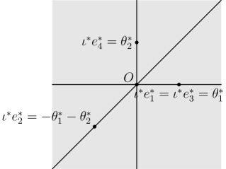
(b) the chamber of same arrangement but different orientation in Example 2.6

Figure 4. two identical chambers, compare with Figure 3

4.3. Extended core and core

In this part, $\beta$ is taken to be zero. It is enough to merely consider the hyperplanes arrangement $H^{1}$. We will abuse the notation using $H$ in stead of $H^{1}$.

The subset of $Y(\alpha,0)$

$$Z=\bar{\mu}_{\mathbb{C}}^{-1}(0)=\{[z,w]\in Y(\alpha,0)|z_{i}w_{i}=0\ \text{for all}\ i\},$$

is called the extended core by Proudfoot(cf. [Pro04]), which naturally breaks into components

$$Z_{\epsilon}=\{[z,w]\in Y(\alpha,0)|w_{i}=0\ if\ \epsilon(i)=1\ and\ z_{i}=0\ if\ \epsilon(i)=-1\}.$$

The variety $Z_{\epsilon}\subset Y(\alpha,0)$ is a $n$-dimensional isotropy Kähler subvariety of $Y(\alpha,0)$ with an effective hamiltonian $T^{n}$-action, hence a toric variety itself. It is not hard to see this is just the toric variety corresponding to the oriented hyperplane arrangement $\mathcal{A}_{\epsilon}$. Denote the associated polytope of $\mathcal{A}_{\epsilon}$ as $\Delta_{\epsilon}$. The set $Z_{cpt}=\bigcup_{\epsilon\in\Theta_{cpt}}Z_{\epsilon}$, where $\Theta_{cpt}=\{\epsilon|\Delta_{\epsilon}\ \text{bounded}\}$, is called the core, union of compact toric varieties $X(\mathcal{A}_{\epsilon}),\epsilon\in\Theta_{cpt}$.

5. Variation of toric hyperkähler variety

5.1. GIT quotient

It’s time to establish the GIT quotient description of toric hyperkähler variety. Consider the GIT quotient of the affine variety $\mu_{\mathbb{C}}^{-1}(\beta)$ by $M_{\mathbb{C}}$ with respect to the linearization on the trivial line bundle induced by $\alpha\in\mathfrak{m}^{*}_{\mathbb{Z}}$. Denote the set of $\alpha$-semi-stable points in $\mu_{\mathbb{C}}^{-1}(\beta)$ by $\mu_{\mathbb{C}}^{-1}(\beta)^{\alpha-ss}$, then there is a categorical quotient $\phi:\mu_{\mathbb{C}}^{-1}(\beta)^{\alpha-ss}\rightarrow\mu_{\mathbb{C}}^{-1}(\beta)^{\alpha-ss}//M_{\mathbb{C}}$. Parallel with toric case, the stability condition can be generalized to any $\alpha\in\mathfrak{m}^{*}$(cf. [Kon08]).

Definition 5.1.

Suppose that $\alpha\in\mathfrak{m}^{*}$,

(1) A point $(z,w)\in\mu_{\mathbb{C}}^{-1}(\beta)$ is $\alpha$-semi-stable if and only if

(5.1) $$\alpha\in\sum^{d}_{i=1}\mathbb{R}_{\geq 0}|z_{i}|^{2}\iota^{*}e_{i}^{*}+\sum^{d}_{i=1}\mathbb{R}_{\geq 0}|w_{i}|^{2}(-\iota^{*}e_{i}^{*}).$$

(2) Suppose $(z,w)\in\mu_{\mathbb{C}}^{-1}(\beta)^{\alpha-ss}$. Then the $M_{\mathbb{C}}$-orbit through $(z,w)$ is closed in $\mu_{\mathbb{C}}^{-1}(\beta)^{\alpha-ss}$ if and only if

(5.2) $$\alpha\in\sum^{d}_{i=1}\mathbb{R}_{>0}|z_{i}|^{2}\iota^{*}e_{i}^{*}+\sum^{d}_{i=1}\mathbb{R}_{>0}|w_{i}|^{2}(-\iota^{*}e_{i}^{*}).$$

And then

Lemma 5.2.

For any point $p\in\mu_{\mathbb{C}}^{-1}(\beta)^{\alpha-ss}//M_{\mathbb{C}}$, the fiber $\phi^{-1}(p)$ consists of finitely many $M_{\mathbb{C}}$-orbits. Moreover, each fiber contains the unique closed $M_{\mathbb{C}}$-orbits in $\mu_{\mathbb{C}}^{-1}(\beta)^{\alpha-ss}$. Thus the categorical quotient $\mu_{\mathbb{C}}^{-1}(\beta)^{\alpha-ss}//M_{\mathbb{C}}$ can be identified with a set of closed $M_{\mathbb{C}}$-orbits in $\mu_{\mathbb{C}}^{-1}(\beta)^{\alpha-ss}$.

Thus we can identify the symplectic quotient $Y(\alpha,\beta)$ with the GIT quotient $\mu_{\mathbb{C}}^{-1}(\beta)^{\alpha-ss}//M_{\mathbb{C}}$ for any $\alpha\in\mathfrak{m}^{*}$.

In the remain part of this subsection, we recall results about variation in [Kon08], and reinterpret them from the perspective of fibred toric variety. We discuss the natural morphism in detail, and the Mukai flop can be viewed as the adjunction of two adjoint natural morphisms.

5.2. Natural morphism and Mukai flop

Under the same set up of toric case, consider the real part chamber structure for a fixed $\beta$, $\alpha_{1}$ is in a generic position of the wall $W_{1}$ and $\alpha^{+}$, $\alpha^{-}$ lie in the chamber $\mathcal{C}^{+}$ and $\mathcal{C}^{-}$ beside the wall. By the definition of stability, we have

$$\mu_{\mathbb{C}}^{-1}(\beta)^{\alpha^{\pm}-ss}\subset\mu_{\mathbb{C}}^{-1}(\beta)^{\alpha_{1}-ss}.$$

Thus this inclusion induces a natural morphism from GIT quotients $\mu_{\mathbb{C}}^{-1}(\beta)^{\alpha^{\pm}-ss}//M_{\mathbb{C}}$ to another GIT quotient $\mu_{\mathbb{C}}^{-1}(\beta)^{\alpha_{1}-ss}//M_{\mathbb{C}}$, which we denote by $\pi^{\pm}:(Y(\alpha^{\pm},\beta),I_{1})\rightarrow(Y(\alpha_{1},\beta),I_{1})$. Without ambiguity we still utilize the notation in toric case. Konno proved Theorem 1.3, and for the reader’s convenience, we give the sketch of proof.

The Proof of Theorem 1.3: (1) Similar with the toric case, $(\alpha_{1},\beta)$ can be considered as a regular element of $\mathfrak{m}_{1}\times\mathfrak{m}_{1\mathbb{C}}$. Likewise $V_{1}$ is a hyperkähler quotient of $\mathbb{H}^{\{1,...,d\}\backslash J_{1}}=\{(z,w)\in\mathbb{H}^{d}|z_{i}=w_{i}=0\ if\ i\in J_{1}\}$ by $M_{1}$.

(2) Choosing $\theta_{1}\in\mathrm{Lie}G_{1}$, by Equation (5.1) we can show that $\mu_{\mathbb{C}}^{-1}(\beta)^{\alpha^{+}-ss}$ is exactly the points in $\mu_{\mathbb{C}}^{-1}(\beta)^{\alpha_{1}-ss}$ satisfying

$$\text{there exists}\ i\in J_{1}\ \text{such that}\ z_{i}\neq 0\ \text{if}\ i\in J^{+}_{1}\ \text{or}\ w_{i}\neq 0\ \text{if}\ i\in J^{-}_{1}.$$

It is also easy to see that, if $(z,w)\in\mu_{\mathbb{C}}^{-1}(\beta)^{\alpha^{+}-ss}$, then

$$[z,w]\in V_{1}\ \text{is equivalent to}\ w_{i}=0\ \text{for}\ i\in J^{+}_{1}\ \text{and}\ z_{i}=0\ \text{for}\ i\in J^{-}_{1}.$$

Thus the fiber of $\pi^{+}|_{V^{+}}:V^{+}\rightarrow V_{1}$ is biholomorphic to $(\mathbb{C}^{\#J_{1}}\backslash\{0\})/G_{1\mathbb{C}}$, i.e. $\mathbb{C}P^{\#J_{1}-1}$. Same thing happens for $\alpha^{-}$.

(3) Same with toric case, reader could consult [Kon08]. ∎

Konno also studied the cross wall phenomena, and show that it turns out to be the Mukai’s elementary transform.

Theorem 5.3.

Assume $\alpha^{+}\in\mathcal{C}^{+}$ and $\alpha^{-}\in\mathcal{C}^{-}$ at different sides of wall $W_{1}$, we can relate $(Y(\alpha^{+},\beta),I_{1})$ to $(Y(\alpha^{-},\beta),I_{1})$ by a Mukai flop. Especially, If $\#J_{1}=2$, there exists a biholomorphic map $\varphi:(Y(\alpha^{+},\beta),I_{1})\rightarrow(Y(\alpha^{-},\beta),I_{1})$ satisfying $\pi^{+}=\pi^{-}\circ\varphi$.

There is no boundary wall and in the interior wall case, toric hyperkähler version is much simpler than the toric one, for all the $J_{1}$ will contribute to the fiber rather than only the $J_{1}^{+}$. Now, we are ready to prove Theorem 1.4, and $\beta$ is set to be zero.

5.3. Relation with fibred toric variety

Take $\beta=0$, consider the natural morphism between $4n$-dimensional toric hyperähler varieties $\pi^{\pm}:Y(\alpha^{\pm},0)\rightarrow Y(\alpha_{1},0)$, it can be encoded as the variation of a regular hyperplane arrangement $\mathcal{A}$ to a non-simplicial one $\mathcal{A}_{1}$. There are some ploytopes belong to the hyperplane arrangement $\mathcal{A}$ vanish in this procedure. These ploytopes are fibred polytopes corresponding to fibred toric varieties. More precisely, the singular set of $\mathcal{A}$ is a $n-(\#J_{1}-1)$ dimensional arrangement $\mathcal{S}$ constituted by $d-\#J_{1}$ hyperplanes, then $V_{1}$ is the toric hyperkähler variety defined by $\mathcal{S}$. Denoting $\tilde{\epsilon}$ a map form $\{1,\dots,d-\#J_{1}\}$ to $\{-1,1\}$, we can state our main theorem as

Theorem.

Let $Z_{1}$ be the extended core of $V_{1}$ which is the toric varieties $X(\mathcal{S}_{\tilde{\epsilon}})$ intersecting together, Restrict $V^{\pm}$ these $\mathbb{C}P^{r}$ fiber bundles to $Z_{1}$, then $V^{\pm}|_{X(\mathcal{S}_{\tilde{\epsilon}})}$ the $\mathbb{C}P^{r}$ fiber bundles over each $X(\mathcal{S}_{\tilde{\epsilon}})$ are all fibred toric varieties of complex dimension $n$.

The proof of Theorem 1.4: Here we only consider $V^{+}$, the $V^{-}$ case is the same. We first show the bundle over $Z_{1}$ lies in the extended core $Z^{+}$ of $Y(\alpha^{+})$. This is merely a repeat of Konno’s proof for (2) of Theorem 1.3. We had already know that $[z,w]\in V^{+}$ is equivalent to $w_{i}=0$ for $i\in J^{+}_{1}$ and $z_{i}=0$ for $i\in J^{-}_{1}$, and the extended core of $V_{1}$ is $\{[z,w]\in\mathbb{H}^{\{1,...,d\}\backslash J_{1}}|z_{i}w_{i}=0,\text{for}\ i\in\{1,...,d\}\backslash J_{1}\}$. Combining these two facts, we know $z_{i}w_{i}=0$ for all $i$, thus the restricted bundle lies in $Z$. Secondly, By Theorem 1.3, $V^{+}$ is complex dimension $2n-2(\#J_{1}-1)$. Hence $X(\mathcal{S}_{\tilde{\epsilon}})$ has half dimension of $V_{1}$, $n-(\#J_{1}-1)$. While its fiber is $(\#J_{1}-1)$-dimensional complex projective space, thus the dimension counting tells us it is complex $n$-dimensional. Finally, the volume of these toric varieties vanishing during the variation, thus must be the fibred toric varieties associated to the fibred polytopes. ∎

This is equivalent to say that the hyperkähler natural morphisms restricted to the toric varieties in the extended core, are the natural morphisms of respect toric varieties. Especially to the fibred toric varieties, the natural morphisms degenerate to bundle projections. As we know, besides the bundle projection of fibred toric varieties, there are lots of ”flip” of toric varieties. Theorem 1.4 tells us that if we look at these flips in its ambient toric hyperkähler variety, then they are all contained in nearby bundle projections of fibred toric varieties. Thus the fibred toric varieties are both primary in the variation of toric varieties and toric hyperkähler varieties. Moreover, Theorem 1.4 directly implies

Corollary 5.4.

Every smooth toric hyperkähler manifold contain fibred toric varieties in its extended core.

We close this article by several examples.

Example 5.5.

We have diagonal action of $T^{1}$ on $\mathbb{H}^{2}$, trying to derive the natural morphism from $Y(1,0)$ to $Y(0,0)$. We already know $Y(1,0)=T^{*}\mathbb{C}P^{1}$. While in the case $\alpha=0$, for the whole affine set $\{z_{1}w_{1}+z_{2}w_{2}=0\}$ is semi-stable, the GIT quotient is just affine quotient. The invariant polynomial ring $K^{T}[z_{1},z_{2},w_{1},w_{2}]/\{z_{1}w_{1}+z_{2}w_{2}\}$ is of form $z_{1}^{p}z_{2}^{q}w_{1}^{r}w_{2}^{s}$ where $p+q=r+s$, which can be generated by $X=z_{1}w_{1}$, $Y=z_{1}w_{2}$, $Z=z_{2}w_{1}$ and $W=z_{2}w_{2}$. Thus the ring is isomorphic to $K[X,Y,Z,W]/\{XW-YZ,X+W\}$, i.e. $K[X,Y,Z]/\{X^{2}+YZ\}$. Its corresponding affine variety is the affine cone $X^{2}+YZ=0$ in $\mathbb{C}^{3}$, isomorphic to $\mathbb{C}^{2}/\mathbb{Z}_{2}$(cf. section 2.2 of [Ful93]). It means that the natural morphism from is just the Klein desigularization of $\mathbb{C}^{2}/\mathbb{Z}_{2}$ to $T^{*}\mathbb{C}P^{1}$.

It is easy to check, the extended core of $Y(1,0)$ is the union of two copies of $\mathbb{C}$ and $\mathbb{C}P^{1}$.

Example 5.6.

Taking $\beta=0$, we consider the fan in Example 2.2, and take $\alpha=3\theta_{1}^{*}+2\theta_{2}^{*}\in\mathcal{C}_{1}$ and $\alpha_{1}=3\theta_{1}^{*}\in W_{1}$, which corresponds to the lifts $\lambda=(1,1,1,1)$ and $\lambda_{1}=(1,1,1,-1)$, then the variation from $\alpha$ to $\alpha_{1}$ is equivalent to moving $H_{4}$ to the superposition of $H_{2}$(see Figure 5). In natural morphism $\pi:Y(\alpha,0)\rightarrow Y(\alpha_{1},0)$, the singular set $V_{1}$ in $Y(\alpha_{1},0)$ is $T^{*}\mathbb{C}P^{1}$, which corresponds to the induced arrangement on the singular set $H_{2}=H_{4}$, with extended core the union of two copies of $\mathbb{C}$ and $\mathbb{C}P^{1}$. The exceptional set $V$ in $Y(\alpha)$ is a $\mathbb{C}P^{1}$ bundle over $T^{*}\mathbb{C}P^{1}$. Restrict it to the extended core, we get two trivial $\mathbb{C}P^{1}$ bundles over $\mathbb{C}$ and a Hirzebrunch surface, which are the fibred toric varieties.

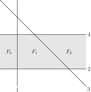
(a) the fibred toric varieties associated

(b) the non-simplicial arrangement, where ploytopes $F_{1}$, $F_{2}$ and $F_{3}$ vanish

Figure 5. variation of arrangement

Craig van Coevering, Email address: craigvan@ustc.edu.cn

Wei Zhang, Email address: zhangw81@ustc.edu.cn

School of Mathematical Sciences

University of Science and Technology of China

Hefei, 230026, P. R.China

References

• [BD00] R. Bielawski and A. Dancer. The geometry and topology of toric hyperkähler manifolds. Commun. Anal. Geom., 8:726–760, 2000.
• [CLS11] D. Cox, J. Little, and H. Schenck. Toric varieties. Graduate Studies in Mathematics. Amer. Math. Soc., Providence, RI, 2011.
• [Del88] T. Delzant. Hamiltioniens periodiques et images convexe de l’application moment. Bull. Soc. Math. France, 116:315–339, 1988.
• [DH98] I. Dolgachev and Y. Hu. Variations of geometric invariant theory quotients. Publ.Math.de l’IHES, 87:5–51, 1998.
• [Dol03] I. Dolgachev. Lectures on Invariant Theory. Cambridge Uni. Press, 2003.
• [Ful93] W. Fulton. Introduction to Toric Varieties. Princeton Uni. Press, 1993.
• [Gui94a] V. Guillemin. Kahler structures on toric varieties. J. Diff. Geom., 40:285–309, 1994.
• [Gui94b] V. Guillemin. Moment Maps and Combinatorial Invariants of Hamiltonian $T^{N}$-spaces. Birkhauser, 1994.
• [HKLR87] N. Hitchin, A. Karlhede, U. Lindstrom, and M. Rocek. Hyperkähler metrics and supersymmetry. Commun. Math. Phys., 108:535–589, 1987.
• [HS02] T. Hausel and B. Sturmfels. Toric hyperkähler varieties. Documenta Mathematica, 7:495–534, 2002.
• [KN78] G. Kempf and L. Ness. On the length of vectors in representation spaces, volume 732 of Lecture Notes in Math. 1978.
• [Kon03] H. Konno. Variation of toric hyperkähler manifolds. International Journal of Mathematics, 14:289–311, 2003.
• [Kon08] H. Konno. The geometry of toric hyperkähler varieties. In Toric Topology, Contemp. Math. 460, pages 241–260, Osaka, 2008.
• [MFK94] D. Mumford, J. Forgaty, and F. Kirwan. Geometric Invariant Theory. Springer, 1994.
• [Nak99] H. Nakajima. Lectures on Hilbert schemes of points on surfaces. American Math. Soc., 1999.
• [Oda88] T. Oda. Convex Bodies and Algebraic Geometry An Introduction to the Theory of Toric Varieties, volume 3 of Ergebnisse der Math. Springer-Verlag, 1988.
• [Pro04] N. Proudfoot. Hyperkähler Analogues of Kahler Quotients. PhD thesis, University of California, Berkeley, 2004.
• [Pro08] N. Proudfoot. A survey of hypertoric geometry and topology. In Toric Topology, Contemp. Math. 460, pages 323–338, Osaka, 2008.
• [Tha96] M. Thaddeus. Geometric invariant theory and flips. J. Amer. Math. Soc., 9(3):691–723, 1996.
• [Tho06] R. Thomas. Notes on GIT and symplectic reduction for bundles and varieties. Arxiv preprint math/0512411, 2006.
• [vCZ11] C. van Coevering and W. Zhang. Cotangent bundles of toric varieties and coverings of toric hyperkähler manifolds. arXiv:1101.5050, 2011.