Weighted genomic distance can hardly impose a bound on the proportion of transpositions
Abstract
Genomic distance between two genomes, i.e., the smallest number of genome rearrangements required to transform one genome into the other, is often used as a measure of evolutionary closeness of the genomes in comparative genomics studies. However, in models that include rearrangements of significantly different “power” such as reversals (that are “weak” and most frequent rearrangements) and transpositions (that are more “powerful” but rare), the genomic distance typically corresponds to a transformation with a large proportion of transpositions, which is not biologically adequate.
Weighted genomic distance is a traditional approach to bounding the proportion of transpositions by assigning them a relative weight . A number of previous studies addressed the problem of computing weighted genomic distance with .
Employing the model of multi-break rearrangements on circular genomes, that captures both reversals (modelled as 2-breaks) and transpositions (modelled as 3-breaks), we prove that for , a minimum-weight transformation may entirely consist of transpositions, implying that the corresponding weighted genomic distance does not actually achieve its purpose of bounding the proportion of transpositions. We further prove that for , the minimum-weight transformations do not depend on a particular choice of from this interval. We give a complete characterization of such transformations and show that they coincide with the transformations that at the same time have the shortest length and make the smallest number of breakages in the genomes.
Our results also provide a theoretical foundation for the empirical observation that for , transpositions are favored over reversals in the minimum-weight transformations.
1 Introduction
Genome rearrangements are evolutionary events that change genomic architectures. Most frequent rearrangements are reversals (also called inversions) that “flip” continuous segments within single chromosomes. Other common types of rearrangements are translocations that “exchange” segments from different chromosomes and fission/fusion that respectively “cut”/“glue” chromosomes.
Since large-scale rearrangements happen rarely and have dramatic effect on the genomes, the number of rearrangements (genomic distance222We remark that the term genomic distance sometimes is used to refer to a particular distance under reversals, translocations, fissions, and fusions.) between two genomes represents a good measure for their evolutionary remoteness and often is used as such in phylogenomic studies. Depending on the model of rearrangements, there exist different types of genomic distance [10].
Particularly famous examples are the reversal distance between unichromosomal genomes [12] and the genomic distance between multichromosomal genomes under all aforementioned types of rearrangements [11]. Despite that both these distances can be computed in polynomial time, their analysis is somewhat complicated, thus limiting their applicability in complex setups. The situation becomes even worse when the chosen model includes more “complex” rearrangement operations such as transpositions that cut off a segment of a chromosome and insert it into some other place in the genome. Computational complexity of most distances involving transpositions, including the transposition distance, remains unknown [13, 4, 8]. To overcome difficulties associated with the analysis of genomic distances many researchers now use simpler models of multi-break [3], DCJ [14], block-interchange [7] rearrangements as well as circular instead of linear genomes, which give reasonable approximation to original genomic distances [1].
Another obstacle in genomic distance-based approaches arises from the fact that transposition-like rearrangements are at the same time much rare and “powerful” than reversal-like rearrangements. As a result, in models that include both reversals and transpositions, the genomic distance typically corresponds to rearrangement scenarios with a large proportion of transpositions, which is not biologically adequate. A traditional approach to bounding the proportion of transpositions is weighted genomic distance defined as the minimum weight of a transformation between two genomes, where transpositions are assigned a relative weight [10]. A number of previous studies addressed the weighted genomic distance for . In particular, Bader and Ohlebusch [4] developed a 1.5-approximation algorithm for . For , Eriksen [9] proposed a -approximation algorithm (for any ).
Employing the model of multi-break rearrangements [3] on circular genomes, that captures both reversals (modelled as 2-breaks) and transpositions (modelled as 3-breaks), we prove that for , a minimum-weight transformation may entirely consist of transpositions. Therefore, the corresponding weighted genomic distance does not actually achieve its purpose of bounding the proportion of transpositions. We further prove that for , the minimum-weight transformations do not depend on a particular choice of from this interval (thus are the same, say, for and ), and give a complete characterization of such transformations. In particular, we show that these transformations coincide with those that at the same time have the shortest length and make the smallest number of breakages in the genomes, first introduced by Alekseyev and Pevzner [2].
Our results also provide a theoretical foundation for the empirical observation of Blanchette et al. [6] that for , transpositions are favored over reversals in the minimum-weight transformations.
2 Multi-break Rearrangements and Breakpoint Graphs
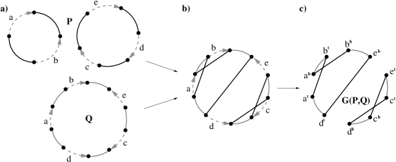
We represent a circular chromosome on genes as a cycle graph on edges alternating between directed “obverse” edges, encoding genes and their directionality, and undirected “black” edges, connecting adjacent genes (Fig. 1a). A genome consisting of chromosomes is then represented as such cycles. The edges of each color form a perfect matching.
A -break rearrangement [3] is defined as replacement of a set of black edges in a genome with a different set of black edges forming matching on the same vertices. In the current study we consider only 2-break (representing reversals, translocations, fissions, fusions) and 3-break rearrangements (including transpositions).
For two genomes and on the same set of genes,333From now on, we assume that given genomes are always one the same set of genes. represented as black-obverse cycles and gray-obverse cycles respectively, their superposition is called the breakpoint graph [5]. Hence, consists of edges of three colors (Fig. 1b): directed “obverse” edges representing genes, undirected black edges representing adjacencies in the genome , and undirected gray edges representing adjacencies in the genome . We ignore the obverse edges in the breakpoint graph and focus on the black and gray edges forming a collection of black-gray alternating cycles (Fig. 1c).
A sequence of rearrangements transforming genome into genome is called transformation. The length of a shortest transformation using -breaks ( or ) is called the -break distance between genomes and .
Any transformation of a genome into a genome corresponds to a transformation of the breakpoint graph into the identity breakpoint graph (Fig. 2). A close look at the increase in the number of black-gray cycles along this transformation, allows one to obtain a formula for the distance between genomes and . Namely, the 2-break distance is related to the number of black-gray cycles in , while the 3-break distance is related to the number of odd black-gray cycles (i.e., black-gray cycles with an odd number of black edges):
Theorem 1 ([14]).
The 2-break distance between genomes and is
Theorem 2 ([3]).
The 3-break distance between genomes and is
3 Breakages and Optimal Transformations
Alekseyev and Pevzner [2] studied the number of breakages444In [2], the term break is used. We use breakage to avoid confusion with -break rearrangements. in transformations. The number of breakages made by a rearrangement is defined as the actual number of edges changed by this rearrangement. A 2-break always makes 2 breakages, while a 3-break can make 2 or 3 breakages. A 3-break making 3 breakages is called complete 3-break. We treat non-complete 3-breaks as 2-breaks.
Alekseyev and Pevzner [2] proved that between any two genomes, there always exists a transformation that simultaneously has the shortest length and makes the smallest number of breakages. We call such transformations optimal.
For a 3-break , we let if makes 3 breakages (i.e., is a complete 3-break) and otherwise. For a transformation , we further define
that is, and are correspondingly the number of 2-breaks and complete 3-breaks in . If 2-breaks and complete 3-breaks are assigned respectively the weights and , then the weight of a transformation is
It is easy to see that a transformation has the length and makes breakages overall. Therefore, a transformation is optimal if and only if it simultaneously minimizes and . We generalize this result in Section 4 by showing that can be replaced with any .
For a rearrangement applied to a breakpoint graph, let and be the resulting increase in the number of respectively odd and even black-gray cycles, respectively. Clearly, gives the increase in the total number of black-gray cycles.
Lemma 3.
For any 3-break ,
-
•
;
-
•
is even and ;
-
•
.
Proof.
A 3-break operating on black edges in the breakpoint graph destroys at least one and at most three black-gray cycles. On the other hand, it creates at least one and at most three new black-gray cycles. Therefore, . Similarly, if , then .
By similar arguments, we also have and .
Since the total number of black edges in destroyed and created black-gray cycles is the same, must be even. Combining this with , we conclude that .
If , then the destroyed cycles must be odd, implying that . However, it is not possible for a 3-break to destroy two cycles and create three new cycles. Hence, . Similarly, , implying that . If (i.e., is a 2-break), similar arguments imply . ∎
Lemma 4.
A transformation between two genomes is shortest if and only if for every . Furthermore, if is a shortest transformation between two genomes, then for every ,
-
•
if , then ;
-
•
if , then or .
Proof.
A transformation of a genome into a genome increases the number of odd black-gray cycles from in to in with the total increase of . By Lemma 3, for every and thus
implying that (i.e., is a shortest transformation) if and only if for every .
Now let be a shortest transformation and thus for every . For a 2-break to have , it must be applied to an even black-gray cycle and split it into two odd black-gray cycles. Thus any such also decreases the number of even black-gray cycles by 1, i.e., .
If a complete 3-break has , then . By Lemma 3, we also have and , implying that or . ∎
By the definition, any optimal transformation is necessarily shortest. However, not every shortest transformation is optimal. The following theorem characterizes optimal transformations within the shortest transformations:
Theorem 5.
A shortest transformation between two genomes is optimal if and only if for any , .
Proof.
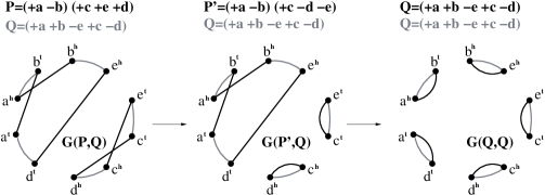
Let be a shortest transformation between two genomes. By Lemma 4, where is the number of complete 3-breaks with and is the number of complete 3-breaks with (Fig. 3).

With 2-breaks and complete 3-breaks is transformed into with trivial black-gray cycles, which are all odd. By Lemma 4, for the increase in the number of odd and even black-gray cycles in the breakpoint graph, we have:
implying that
which is minimal if and only if , i.e., for any . ∎
Corollary 6.
A transformation between two genomes is optimal if and only if for any ,
-
•
if , then and ;
-
•
if , then and .
Theorem 7.
A transformation between genomes and is optimal if and only if
| (1) |
Proof.
Let be an optimal transformation between genomes and . Then with 2-breaks and complete 3-breaks, it transforms into with trivial black-gray cycles, which are all odd. By Corollary 6, we have
implying formulae (1).
Vice versa, a transformation between genomes and , satisfying (1), has the length , implying that is a shortest transformation. By Lemma 4, for every 2-break and or for every complete 3-break . Let be the number of complete 3-breaks with . Then the increase in the number of even black-gray cycles along is
implying that and thus is optimal by Theorem 5. ∎
Theorem 7 implies that for some genomes, every optimal transformation consists entirely of complete 3-breaks:
Corollary 8.
For genomes and with , every optimal transformation has and thus consists entirely of complete 3-breaks.
Corollary 9.
For an optimal transformation between genomes and ,
4 Weighted multi-break distance
Let be the set of all transformations between genomes and . For a real number , we define the weighted distance between genomes and as
that is, the minimum possible weight of a transformation between and .
Two important examples of the weighted distance are the “unweighted” distance and the distance equal the half of the minimum number of breakages in a transformation between genomes and . By the definition of an optimal transformation, we have , where is an optimal transformation between genomes and . Below we prove that for any .
Theorem 10.
For ,
where is any optimal transformation between genomes and .
Furthermore, for , if for a transformation between genomes and , then is an optimal transformation.
Proof.
Let be any transformation and be any optimal transformation between genomes and .
We classify all possible changes in the number of even and odd black-gray cycles resulted from a single rearrangement . By Lemma 3, may take only values , while (if is a 2-break) or (if is a complete 3-break). The table below lists the possible values of and , satisfying these restrictions, along with the amount of rearrangements of each particular type in , denoted for 2-breaks and for complete 3-breaks.
| 0 | 0 | 0 | -2 | 2 | 0 | 0 | 0 | 0 | 0 | 2 | 2 | 2 | -2 | -2 | -2 | |
| 0 | 1 | -1 | 1 | -1 | 0 | 1 | -1 | 2 | -2 | 0 | -1 | -2 | 0 | 1 | 2 | |
| amount in | ||||||||||||||||
For the transformation , we have
Calculating the total increase in the number of odd and even black-gray cycles along , we have
Theorem 7 further implies
Now we can evaluate the difference between the weights of and as follows:
Since and , all summands in the last expression are nonnegative and thus . Since is an arbitrary transformation, we have
For , if then , implying that only and (appearing with zero coefficients in the expression for ) can be nonzero and thus is optimal by Corollary 6. ∎
5 Discussion
We proved that for , the minimum-weight transformations include the optimal transformations (Theorem 10) that may entirely consist of transposition-like operations (modelled as complete 3-breaks) (Corollary 8). Therefore, the corresponding weighted genomic distance does not actually impose any bound on the proportion of transpositions.
For , we proved even a stronger result that the minimum-weight transformations coincide with the optimal transformations (Theorem 10). As a consequence we have that a particular choice of imposes no restrictions for the minimum-weight transformations as compared to other values of from this interval. The value then proves that the optimal transformations coincide with those that at the same time have the shortest length and make the smallest number of breakages, studied by Alekseyev and Pevzner [2]. We further characterized the optimal transformations within the shortest transformations (i.e., the minimum-weight transformations for ) by showing that the optimal transformations avoid one particular type of rearrangements (Theorem 5, Fig. 3).
It is worth to mention that the weighted genomic distance with is useless, since it allows (for ) or even promotes (for ) replacement of every complete 3-break with two equivalent 2-breaks, thus eliminating complete 3-breaks at all.
The extension of our results to the case of linear genomes will be published elsewhere.
References
- [1] Alekseyev, M. A. Multi-Break Rearrangements and Breakpoint Re-uses: from Circular to Linear Genomes. Journal of Computational Biology 15, 8 (2008), 1117–1131.
- [2] Alekseyev, M. A., and Pevzner, P. A. Are There Rearrangement Hotspots in the Human Genome? PLoS Computational Biology 3, 11 (2007), e209.
- [3] Alekseyev, M. A., and Pevzner, P. A. Multi-Break Rearrangements and Chromosomal Evolution. Theoretical Computer Science 395, 2-3 (2008), 193–202.
- [4] Bader, M., and Ohlebusch, E. Sorting by weighted reversals, transpositions, and inverted transpositions. Journal of Computational Biology 14, 5 (2007), 615–636.
- [5] Bafna, V., and Pevzner, P. A. Genome rearrangements and sorting by reversals. SIAM Journal on Computing 25 (1996), 272–289.
- [6] Blanchette, M., Kunisawa, T., and Sankoff, D. Parametric genome rearrangement. Gene 172, 1 (1996), GC11 – GC17.
- [7] Christie, D. A. Sorting permutations by block-interchanges. Information Processing Letters 60, 4 (1996), 165 – 169.
- [8] Elias, I., and Hartman, T. A 1.375-approximation algorithm for sorting by transpositions. IEEE/ACM Transactions on Computational Biology and Bioinformatics 3 (2006), 369–379.
- [9] Eriksen, N. -Approximation of Sorting by Reversals and Transpositions. Lecture Notes in Computer Science 2149 (2001), 227–237.
- [10] Fertin, G., Labarre, A., Rusu, I., and Tannier, E. Combinatorics of Genome Rearrangements. The MIT Press, 2009.
- [11] Hannenhalli, S., and Pevzner, P. Transforming men into mouse (polynomial algorithm for genomic distance problem). Proceedings of the 36th Annual Symposium on Foundations of Computer Science (1995), 581–592.
- [12] Hannenhalli, S., and Pevzner, P. A. Transforming Cabbage into Turnip (polynomial algorithm for sorting signed permutations by reversals). In Proceedings of the 27th Annual ACM Symposium on the Theory of Computing (1995), pp. 178–189. (full version appeared in Journal of ACM, 46: 1–27, 1999).
- [13] Radcliffe, A. J., Scott, A. D., and Wilmer, E. L. Reversals and Transpositions Over Finite Alphabets. SIAM J. Discrete Math. 19 (2005), 224–244.
- [14] Yancopoulos, S., Attie, O., and Friedberg, R. Efficient sorting of genomic permutations by translocation, inversion and block interchange. Bioinformatics 21 (2005), 3340–3346.