Horizon area–angular momentum inequality for a class of axially symmetric black holes

Abstract

We prove an inequality between horizon area and angular momentum for a class of axially symmetric black holes. This class includes initial conditions with an isometry which leaves fixed a two-surface. These initial conditions have been extensively used in the numerical evolution of rotating black holes. They can describe highly distorted black holes, not necessarily near equilibrium. We also prove the inequality on extreme throat initial data, extending previous results.

1 Introduction

In a recent article [11] the following conjecture was formulated:

Conjecture 1.1.

Consider an asymptotically flat, vacuum, complete axially symmetric initial data set for Einstein equations. Then the following inequality holds

$$8\pi|J|\leq A,$$ (1)

where $A$ and $J$ are the area and angular momentum of a connected component of the apparent horizon.

See [11] for a physical interpretation and motivation of the inequality (1). In that article evidences for the validity of conjecture 1.1 were presented. These evidences are the following: in a particular class of initial data set, called extreme throat initial data, the first variation of the area, with fixed angular momentum, is zero and the second variation is positive definite evaluated at the extreme Kerr throat initial data. This indicates that the area of the extreme Kerr throat initial data is a minimum among this class of data. Since extreme Kerr initial data satisfy the equality in (1) it follows that the area of generic throat initial data satisfies (1). The key ingredient for this analysis is a formula that relates the variations of the area of extreme throat initial data with the variation of an appropriately defined mass functional.

However, as it was pointed out in [11], in order to use these arguments to prove conjecture 1.1, there are two main points that need to be addressed. The first one is the following. It is well known that a non-negative second variation is a necessary condition for a local minimum but it is not sufficient. To prove that extreme Kerr is a local minimum it is necessary to provide extra estimates in a similar way as in [9]. As remarked in [11] it is expected that the same analysis will apply to this case also. However, to prove that extreme Kerr is a global minimum (which is, of course, what we need to prove) a different ingredient is needed, since it is a priori not clear how to relate the area and the mass functional mentioned above far from the extreme Kerr solution.

The second point is how to extend the result on extreme throat initial data to include the physically relevant asymptotically flat black hole initial data mentioned in the conjecture. In [11] a limit procedure was proposed which could in principle reduce the general case to the extreme throat case. This limit procedure is similar in spirit to the extreme limit of the Kerr black hole initial data. However, it is far from clear how to construct this limit in general. A natural candidate would be initial data which are close to Kerr. Even for that class of data the construction appears to be difficult.

The purpose of this article is to address the two points mentioned above. For the first one we give a complete and optimal answer, namely, we prove that extreme Kerr throat initial data are a global minimum in this class. At the core of our argument lies a remarkable inequality that relates the area and the mass functional for extreme throat initial data. This inequality is the global generalization of the local arguments presented in [11].

For the second point we give a partial answer. We prove the conjecture for a class of initial data which has several technical restrictions. However, despite of that, this class is relevant by itself. It includes initial data which have an isometry that leaves fixed a two-dimensional surface. This kind of data can describe distorted rotating black holes far from equilibrium. They have been extensively used in numerical simulations [3]. The well known Bowen-York family of initial data [2] is a particular case, where the metric is conformally flat. Our proof does not rely on a limit procedure. Remarkable enough, it is a pure local argument, which uses the mass formula to estimate in a simple fashion the area of the minimal surface.

Finally, we extend the validity of conjecture 1.1 to include a non-negative cosmological constant (and hence non-asymptotically flat initial data). This generalization is relevant because there exists a counter-example of inequality (1) for the case of negative cosmological constant, as it was pointed out in [1]. It will be seen that the inclusion of the cosmological constant stresses the role of a non-negative Ricci scalar.

The plan of the article is the following. In section 2 we present our main result, given by theorem 2.1. We also discuss the scope of the theorem and analyze relevant examples. The proof of this result consists of two main parts, explained in sections 3 and 4.

The main result of section 3 is an estimate for the area in terms of the mass functional. In section 4 we present a variational argument that asserts that the global minimum of the mass functional is given by the extreme throat Kerr initial data.

2 Main Result

An initial data set for Einstein equations, with cosmological constant $\Lambda$, consists in a Riemannian 3-manifold $S$, together with its first and second fundamental forms, $h_{ij}$ and $K_{ij}$ respectively, which satisfy the vacuum Einstein constraints on $S$

$$R+K^{2}-K_{ij}K^{ij} =2\Lambda,$$ (2)

$$\nabla^{i}K_{ij}-\nabla_{j}K =0.$$ (3)

In these equations, $K=h^{ij}K_{ij}$, the Ricci scalar $R$, the contractions and covariant derivatives are computed with respect to $h_{ij}$. The presence of the cosmological constant $\Lambda$ allows for non asymptotically flat data describing initial data of de Sitter ($\Lambda>0$) or anti-de Sitter ($\Lambda<0$) type.

When the initial data are maximal (i.e. $K=0$) the constraint equations simplify considerably. In particular, when $\Lambda\geq 0$, the scalar curvature $R$ is non-negative. The condition $R\geq 0$ plays a crucial role in this article.

The initial data are axially symmetric if there exists an axial Killing vector field $\eta^{i}$ such that

$$\mathcal{L}_{\eta}h_{ij}=0,\qquad\mathcal{L}_{\eta}K_{ij}=0,$$ (4)

where $\mathcal{L}$ denotes the Lie derivative. The Cauchy development of such initial data will be an axially symmetric spacetime.

For an axially symmetric metric, it is always possible [4] to choose local coordinates ($r,\theta,\phi$) such that

$$h=e^{\sigma}\left[e^{2q}(dr^{2}+r^{2}d\theta^{2})+r^{2}\sin^{2}\theta(d\phi+v_{r}dr+v_{\theta}d\theta)^{2}\right],$$ (5)

where $\sigma,q,v_{r}$ and $v_{\theta}$ are regular functions of $r$ and $\theta$. In these coordinates, the Killing vector is given by

$$\eta^{i}=(\partial_{\phi})^{i},$$ (6)

and its square norm is

$$\eta=\eta^{i}\eta_{i}=e^{\sigma}r^{2}\sin^{2}\theta.$$ (7)

The regularity conditions on the metric $h$ at the axis imply that

$$q|_{\Gamma}=0,$$ (8)

where $\Gamma$ denotes the polar axis $r\sin\theta=0$.

The twist potential $\omega$ of the spacetime axial Killing field can be computed in terms of the second fundamental form $K_{ij}$ as follows (see [10] for details). Define the vector $S^{i}$ by

$$S_{i}=K_{ij}\eta^{j}-\eta^{-1}\eta_{i}K_{jk}\eta^{j}\eta^{k},$$ (9)

then, define $K_{i}$ by

$$K_{i}=\epsilon_{ijk}S^{j}\eta^{k},$$ (10)

where $\epsilon_{ijk}$ is the volume element with respect to the flat metric. In virtue of the constraint equations, the vector $K_{i}$ is the gradient of a scalar field which is the twist potential, namely

$$K_{i}=\frac{1}{2}\nabla_{i}\omega.$$ (11)

In this work, we will study the geometry of the 2-surfaces $r=constant$. For these surfaces there exist two relevant quantities. The first one is the angular momentum, which for such surfaces is defined by

$$J=\frac{1}{8}\left(\omega(r,\theta=\pi)-\omega(r,\theta=0)\right).$$ (12)

See [10] for a detailed discussion about angular momentum in axial symmetry.

The second quantity is the area of the surface. The induced 2-metric on such surfaces is

$$\gamma=e^{\sigma}r^{2}\left[e^{2q}d\theta^{2}+\sin^{2}\theta(d\phi+v_{\theta}d\theta)^{2}\right],$$ (13)

and, remarkably, its determinant does not depend on $v_{\theta}$ or $v_{r}$,

$$\det(\gamma)=e^{2\sigma+2q}r^{4}\sin^{2}\theta.$$ (14)

Then, the area of the surface $r=constant$ is given by

$$A=\int_{S^{2}}\sqrt{\det(\gamma)}d\theta d\phi=\int_{S^{2}}e^{\sigma+q}r^{2}dS=2\pi r^{2}\int_{0}^{\pi}e^{\sigma+q}\sin\theta d\theta,$$ (15)

where $dS=\sin\theta d\theta d\phi$ is the surface element on the unit 2-sphere and in the last equality we have made use of axial symmetry.

Another useful geometrical quantity is the second fundamental form $\chi_{ij}$ of the surface given by

$$\chi_{ij}=-\gamma_{i}^{k}\nabla_{k}n_{j}$$ (16)

where $n_{i}=e^{\sigma/2+q}(dr)_{i}$ is the unit normal to the surface. The mean curvature of the surface is an important concept in what follows and reads

$$\chi=\chi^{i}_{i}=e^{-\sigma/2-q}\left(\partial_{r}(\sigma+q)+\frac{2}{r}\right),$$ (17)

The mean curvature $\chi$ is related with the radial derivatives of the area $A$ as follows. For the first derivative we have

$$\partial_{r}A=\int_{S^{2}}e^{\frac{3}{2}\sigma+2q}r^{2}\chi\,dS,$$ (18)

and for the second derivative,

$$\partial_{r}^{2}A=\int_{S^{2}}\left[e^{\frac{3}{2}\sigma+2q}r^{2}\partial_{r}\chi+\chi\partial_{r}(r^{2}e^{\frac{3}{2}\sigma+2q})\right]\,dS.$$ (19)

The case $\chi=0$ will be relevant for our purposes. For that case we have

$$\partial_{r}^{2}A=\int_{S^{2}}e^{\frac{3}{2}\sigma+2q}r^{2}\partial_{r}\chi\,dS.$$ (20)

The following theorem constitutes the main result of the present work.

Theorem 2.1.

Consider axisymmetric, vacuum and maximal initial data, with a non-negative cosmological constant as described above. Assume there exists a surface $\Sigma=\{r=constant\}$ where the following local conditions are satisfied

$$\chi =0,$$ (21)

$$\partial_{r}\chi \geq 0,$$ (22)

$$\partial_{r}q =0.$$ (23)

Then we have

$$8\pi|J|\leq A$$ (24)

where $A$ is the area and $J$ the angular momentum of $\Sigma$.

Let us discuss the hypothesis of this theorem. The theorem is a pure local result, in particular there are no conditions on the asymptotics of the initial data. We have also introduced the cosmological constant, generalizing in this way the validity of conjecture 1.1. As we mention in the introduction, in [1] it has been presented a counter example to inequality (1) with negative cosmological constant. Maximal data with non-negative cosmological constant (as required in the hypothesis of the theorem) have non-negative Ricci scalar. This is the crucial property that allows us to prove (24).

The first important restriction of the theorem is that only surfaces $r=constant$ are allowed. In the general case, the horizon mentioned in the conjecture will not be such a surface. This particular choice of foliation adapted to the cylindrical coordinates simplifies considerably the estimates. A relevant open problem is how to extend these results to include general surfaces.

By equations (18) and (20), we deduce that conditions (21) and (22) imply that the area of the surface $\Sigma$ is a local minimum. That is, $\Sigma$ is a minimal surface . If these were the only hypothesis in the theorem, then conjecture 1.1 would be proved for initial data having a global minimal surface $r=constant$: by definition, the area of such minimal surface is less than or equal to the area of any surface, the horizon in particular. However, in order to prove the inequality (24) we require the extra condition (23). This is a technical condition which we do not expect to be necessary. However, it is important to emphasize that this is also a geometrical condition, since it can be written in terms of $\chi$ and the component $\chi_{ij}\eta^{i}\eta^{j}$ of the extrinsic curvature $\chi_{ij}$ of $\Sigma$, namely

$$\chi=0\qquad\mbox{and}\qquad\chi_{ij}\eta^{i}\eta^{j}=0\qquad\Rightarrow\qquad\partial_{r}q=0.$$ (25)

This result can be seen in the following way

$$\chi_{ij}\eta^{i}\eta^{j}=-\gamma^{k}_{i}\nabla_{k}n_{j}\eta^{i}\eta^{j}=-\nabla_{i}n_{j}\eta^{i}\eta^{j}=-\nabla_{i}(n_{j}\eta^{j})\eta^{i}+n_{j}(\nabla_{i}\eta^{j})\eta^{i},$$ (26)

but the first term in the last expression is zero because $\eta^{i}$ and $n_{i}$ are orthogonal. Then

$$\chi_{ij}\eta^{i}\eta^{j}=n^{j}(\nabla_{i}\eta_{j})\eta^{i}=-n^{j}(\nabla_{j}\eta_{i})\eta^{i}$$ (27)

since $\eta^{i}$ is a Killing vector field. Finally we have

$$\chi_{ij}\eta^{i}\eta^{j}=-\frac{1}{2}n^{j}\nabla_{j}\eta=-\frac{1}{2}n^{r}\partial_{r}\eta=-\frac{1}{2}n^{r}r^{2}\sin^{2}\theta e^{\sigma}\left(\partial_{r}\sigma+\frac{2}{r}\right),$$ (28)

where, in the second equality, we have made use of axial symmetry. Therefore, $\chi_{ij}\eta^{i}\eta^{j}=0$ together with $\chi=0$, imply $\partial_{r}q=0$ (see equation (17)).

This alternative way of writing the hypotheses of theorem 2.1 gives a more geometrical description of the surface considered. In particular, totally geodesic surfaces (i.e. surfaces such that $\chi_{ij}=0$) satisfy (25) and (21). Moreover, when $v_{r}\equiv v_{\theta}\equiv 0$, condition (25) implies that $\Sigma$ is totally geodesic.

There exists a particularly relevant class of initial data that satisfies all conditions imposed in theorem 2.1. Namely, initial data with an isometry that leaves the surface $\Sigma$ invariant. This isometry is also called “inversion through the throat” in the literature. Let us discuss this family of examples in more detail.

In [16] it has been proven that a compact 2-surface that is invariant under an isometry is a totally geodesic surface. Note that the isometry only imposes conditions on the first order derivatives of the initial data functions evaluated at the invariant surface $\Sigma$. Condition (22), which is a condition on the second derivatives of the metric, is not automatically satisfied. In fact, a surface could be a local maximum and still be invariant under the isometry. However, for a rich class of data this surface is a global minimum. To analyze this point it is better to discuss concrete examples.

A canonical example of this kind of isometric data is a slice $t=constant$ (in the standard Boyer-Lindquist coordinates) of the non-extreme Kerr black hole. The geometry of these data (which is the same as the Schwarzschild black hole) is the well known picture shown in figure 1. The global minimal surface that connects the two sheets satisfies all the hypothesis of the theorem. In this case the minimal surface coincides with the apparent horizon. The Kerr black hole initial data constitute a non-trivial example of the theorem. Although inequality (24) can be of course computed explicitly for Kerr, the theorem presents an alternative proof of it.

For more general black hole initial data, isometry conditions were introduced in [19] and since then they have been extensively used to construct initial data for black hole numerical simulations. A well known example is the conformally flat (i.e. $q=0$) family of black hole initial data introduced by Bowen and York [2]. Another conformally flat case was analyzed in [14]. Non-conformally flat examples have been studied in [3]. In all these examples black hole initial data with the geometry shown in figure 1 have been constructed. These data represent distorted black holes and can, in principle, be far from equilibrium. However, it is important to emphasize that in order for the isometry invariant surface $\Sigma$ to remain a global minimum of the area the distortion should not produce extra minimal surfaces, as in the case shown in figure 2. In that case the theorem still applies for the surface $\Sigma$ but since it is does not give the global minimum of the area, we can not prove the conjecture.

Conditions ensuring that the isometry surface gives a minimum for the area have been studied for some examples in [2]. There exists also a lot of numerical evidence for all these examples showing that if the distortion from Kerr is not too severe, then the isometry surface gives in fact a global minimum for the area (for example, see [7]). It is interesting to note that in many of these examples the horizon and the minimal surface do not coincide [7]. Also, this kind of isometry data can represent binary black hole initial data (this is in fact one of the main applications of these data, see [19], [2])). In the case of binary black holes, there exist two minimal surfaces which are invariant under the isometry. Remarkable enough, these surfaces also satisfy conditions (21), (22) and (23). But they are not $r=constant$ surfaces, and hence the theorem does not apply to them.

It is also important to mention that the isometry condition is preserved under the evolution (in fact it has been explicitly used for numerical evolution, see [3]) and hence it can play a useful role in the analytical study of the black hole stability problem for this kind of data.

We summarize the above discussion in the following corollary.

Corollary 2.2.

Consider axisymmetric, vacuum and maximal initial data, with a non-negative cosmological constant as described above. Assume there exists an isometry which leaves fixed a surface $\Sigma=\{r=constant\}$. Assume also that the area of this surface is a global minimum. Then conjecture 1.1 is proven for these data.

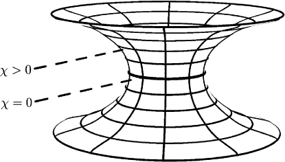
Figure 1: Initial data with an isometry. The data have a global minimal surface in the middle. The conjecture 1.1 is proven for this kind of data.

Figure 2: An example of data with an isometry. The theorem applies to the minimal surface in the middle, but the conjecture can not be proven in this case because there are other minimal surfaces with less area.

There exists another class of initial data that is not strictly included in the formulation of conjecture 1.1, but which plays an important role in the proof as a limit case. And also, it could have further interesting applications. These are the extreme throat initial data introduced in [11]. This kind of data is a special case of axially symmetric data discussed above where an additional symmetry is present. In order to introduce them, it is convenient to make the change of coordinates $s=-\ln r$ to the metric (5). We also define the function $\varsigma$ by

$$\varsigma=\sigma+2\ln r.$$ (29)

Then, the line element (5) is written as

$$h=e^{\varsigma}\left[e^{2q}(ds^{2}+d\theta^{2})+\sin^{2}\theta(d\phi+v_{s}ds+v_{\theta}d\theta)^{2}\right].$$ (30)

Assume that $\varsigma$, $q$, $v_{s}$ and $v_{\theta}$ do not depend on $s$, then $\partial_{s}$ is a Killing vector of $h$ (besides $\partial_{\phi}$). If also $\mathcal{L}_{\partial_{s}}K_{ij}=0$ then we call $(S,h_{ij},K_{ij})$ an extreme throat initial data set. The geometry of these data is cylindrical (see figure 3), as $S$ is $S^{2}\times\mathbb{R}$ and the sections $s=constant$ are topological spheres which are isometric to each other.

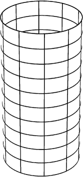
Figure 3: Cylindrical geometry of extreme throat initial data.

For these data the twist potential $\omega$ is defined in the same way as done for general axially symmetric data, and now it is a function that depends only on $\theta$. As the data are symmetric with respect to translations in the $s$ direction, the angular momentum and area associated with these data do not depend on $s$. They are given by

$$J=\frac{1}{8}(\omega(\pi)-\omega(0)),$$ (31)

$$A=2\pi\int_{0}^{\pi}e^{\varsigma+q}\sin\theta\,d\theta,$$ (32)

which are the corresponding expressions to (12) and (15).

A particularly relevant functional for this class of data is the mass functional ${\cal M}$, defined as (see [11])

$${\cal M}=\int_{0}^{\pi}\left(|\partial_{\theta}\varsigma|^{2}+4\varsigma+\frac{|\partial_{\theta}\omega|^{2}}{\eta^{2}}\right)\sin\theta\,d\theta.$$ (33)

This functional plays a fundamental role in the proof of theorem 2.1 and has two important properties. The first one is that it is possible to relate it with the area $A$. The second property is that it is essentially equivalent to the energy of an harmonic map. Both properties will constitute the core of the proof of theorem 2.1, they will be explained in sections 3 and 4 respectively.

Note that by the non-dependence on $s$ (and hence on $r$) of the functions, conditions (21), (22) and (23) are satisfied for extreme throat initial data. Hence we have the following corollary of theorem 2.1.

Corollary 2.3.

For an extreme throat initial data set the inequality

$$8\pi|J|\leq A.$$ (34)

holds, where $A$ and $J$ are the area and angular momentum of the data given by (31) and (32).

This corollary significantly extends the results presented in [11] in two directions. First, it applies to general extreme throat initial data. The Killing vector $\partial_{s}$ is not required to be hypersurface orthogonal. In fact, the result applies to a slightly more general class of data, the only condition required is that the functions $\varsigma$, $q$ and $\omega$ do not depend on $s$. But no condition is imposed on $v_{s}$ and $v_{\theta}$. These functions could depend on $s$, in that case the data will not admit the Killing field $\partial_{s}$ but the corollary will still hold.

The second extension with respect to [11] is that this is a global result and not a local one. As we mentioned in the introduction, to prove this result we will use a remarkable inequality relating the area and the mass functional. This is explained in section 3.

The importance of extreme throat initial data resides on that they naturally appear as the limit geometry of initial data with a cylindrical end. The canonical example of these data is the extreme Kerr black hole initial data. See figure 4 for a representation of the geometry of these data. At the cylindrical end, all the derivatives with respect to $r$ of the relevant functions decay to zero, but not the functions themselves. They have a well defined limit. These limit functions define extreme throat initial data (for the details of this construction see [11]).

Remarkably, the previous corollary applies to the limit area of the cylindrical end of extreme black hole initial data. This limit area is not directly related with conjecture 1.1 because it is not a horizon. But it still has interesting applications. Extreme Kerr is of course an example, where the equality holds. But there are also other examples as the ones constructed in [15] [13] [6] [12].

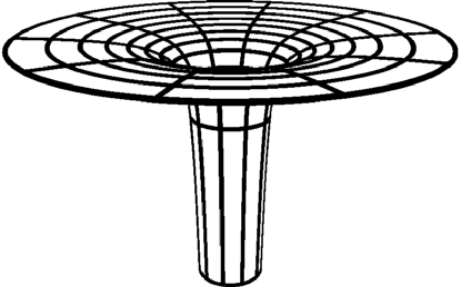
Figure 4: Geometry of extreme black hole initial data. The data have an asymptotically flat end (top) and a cylindrical end (bottom).

Finally, we present the proof of theorem 2.1.

Proof of theorem 2.1.

The proof is divided into two main parts described in sections 3 and 4. First we obtain an inequality relating the area with the mass functional. This is given by lemma 3.2. Here, we have made use of hypothesis (21), (22) and (23). Then, using lemma 4.1 we bound the mass functional by the angular momentum and we obtain the desired result. ∎

3 Area and mass functional

The purpose of this section is to get a lower bound on the area $A$ of the surface $\Sigma$ mentioned in theorem 2.1 in terms of the mass functional (33). All the calculations that follow are local, no asymptotic behavior being assumed.

The Hamiltonian equation (2), together with the maximality condition, $K=0$, give

$$R=K_{ij}K^{ij}+2\Lambda.$$ (35)

In [10] it has been proven that

$$K_{ij}K^{ij}\geq\frac{1}{2}\frac{|\partial\omega|^{2}}{\eta^{2}}e^{-\sigma-2q},$$ (36)

where $\omega$ is the twist potential introduced in (11). By inserting (36) in (35) and using the condition $\Lambda\geq 0$, one gets the bound

$$R\geq\frac{1}{2}\frac{|\partial\omega|^{2}}{\eta^{2}}e^{-\sigma-2q}.$$ (37)

The Ricci scalar $R$ in terms of the metric functions $\sigma$, $q$, $v_{r}$ and $v_{\theta}$ is

$$R=-2e^{-\sigma-2q}\Bigg{(}\Delta\sigma+\Delta_{2}q+\frac{1}{4}|\partial\sigma|^{2}+\frac{1}{4}\sin^{2}\theta e^{-2q}(v_{r,\theta}-v_{\theta,r})^{2}\Bigg{)},$$ (38)

where $\Delta$ and $\Delta_{2}$ are the flat Laplace operators in three and two dimensions respectively, and $\partial$ denotes partial derivatives. From (37) and (38) we finally obtain

$$|\partial\sigma|^{2}+\frac{|\partial\omega|^{2}}{\eta^{2}}\leq-4\left(\Delta\sigma+\Delta_{2}q\right).$$ (39)

We write this inequality explicitly in spherical coordinates and arrange terms in the following useful way

$$(\partial_{\theta}\sigma)^{2}+\frac{(\partial_{\theta}\omega)^{2}}{\eta^{2}}\leq-4(\partial_{\theta}^{2}q+\Delta_{0}\sigma)-f-g$$ (40)

where $\Delta_{0}$ is the Laplace operator on $S^{2}$ acting on axially symmetric functions

$$\Delta_{0}\sigma=\frac{1}{\sin\theta}\partial_{\theta}(\sin\theta\partial_{\theta}\sigma),$$ (41)

and

$$f=4r^{2}\partial^{2}_{r}(\sigma+q),$$ (42)

$$g=4r\partial_{r}(2\sigma+q)+r^{2}(\partial_{r}\sigma)^{2}+r^{2}\frac{(\partial_{r}\omega)^{2}}{\eta^{2}}.$$ (43)

Now we integrate (40) in the unit 2-sphere. Using

$$\int_{S^{2}}\Delta_{0}\sigma dS=0$$ (44)

and (see [11])

$$\int_{S^{2}}\partial_{\theta}^{2}qdS=-\int_{S^{2}}qdS,$$ (45)

we obtain

$$\int_{S^{2}}(\partial_{\theta}\sigma)^{2}+\frac{(\partial_{\theta}\omega)^{2}}{\eta^{2}}dS\leq 4\int_{S^{2}}qdS-F-G,$$ (46)

where we have defined

$$F=\int_{S^{2}}fdS,\qquad G=\int_{S^{2}}gdS.$$ (47)

In order to make contact with the mass functional $\mathcal{M}$, we write the left hand side of inequality (46) in terms of $\varsigma$, defined in (29),

$$\int_{S^{2}}(\partial_{\theta}\varsigma)^{2}+\frac{(\partial_{\theta}\omega)^{2}}{\eta^{2}}dS\leq 4\int_{S^{2}}qdS-F-G.$$ (48)

Adding up a term of the form $4\int_{S^{2}}\varsigma dS$ to both sides of (48) we obtain an upper bound for $\mathcal{M}$,

$$2\pi\mathcal{M}\leq 4\int_{S^{2}}(\varsigma+q)dS-F-G.$$ (49)

This is more conveniently written as

$$\frac{\mathcal{M}}{8}+\frac{F+G}{16\pi}\leq\frac{1}{2}\int_{0}^{\pi}(\varsigma+q)\sin\theta d\theta,$$ (50)

where we have integrated the right hand side over $\phi$. For our purposes later, it is useful to exponentiate the above inequality

$$e^{\frac{\mathcal{M}}{8}}e^{\frac{F+G}{16\pi}}\leq e^{\frac{1}{2}\int_{0}^{\pi}(\varsigma+q)\sin\theta d\theta}.$$ (51)

We want to remark that in going from (46) to (48) there appears to be an inconsistency concerning units. Nevertheless, since in the end we take the exponential of that inequality, the final result, (51), has the right dimension of area.

We want to use this inequality to bound the area of the surfaces $r=constant$. We write the area for these surfaces in the form (see equation (15))

$$\frac{A}{4\pi}=\frac{1}{2}\int_{0}^{\pi}e^{\varsigma+q}\sin\theta d\theta,$$ (52)

then, using Jensen’s inequality for the exponential function we have

$$\frac{1}{2}\int_{0}^{\pi}e^{\varsigma+q}\sin\theta d\theta\geq e^{\frac{1}{2}\int_{0}^{\pi}\varsigma+q\sin\theta d\theta}$$ (53)

which gives

$$\frac{A}{4\pi}\geq e^{\frac{1}{2}\int_{0}^{\pi}\varsigma+q\sin\theta d\theta}.$$ (54)

Finally, we put together inequalities (51) and (54) to obtain

$$A\geq 4\pi e^{\frac{\mathcal{M}}{8}}e^{\frac{F+G}{16\pi}},$$ (55)

and this gives a bound for the area of the surface $r=constant$ through the functional $\mathcal{M}$ and radial derivatives of $\sigma$ and $q$.

This result proves the following lemma.

Lemma 3.1.

The area $A$ of a surface $r=constant$ satisfies inequality (55), where $F$ and $G$ are defined in (47) and $\mathcal{M}$ is evaluated at $r$.

We remark that in order to get inequality (55) we have only made use of the Hamiltonian constraint, the maximality condition, the positivity of the cosmological constant $\Lambda$ and the bound (36) for the square of the extrinsic curvature. Moreover, it holds for any surface $r=constant$.

Inequality (55) is the crucial ingredient in proving the following lemma.

Lemma 3.2.

If conditions (21)-(23) of theorem 2.1 hold for the surface $\Sigma$ of constant $r$, then its area $A$ satisfies

$$A\geq 4\pi e^{\frac{(\mathcal{M}-8)}{8}}$$ (56)

where $\mathcal{M}$ is the mass functional (33) evaluated at the surface $\Sigma$.

Proof.

Take inequality (55) and evaluate it at the particular surface $\Sigma$ mentioned in theorem 2.1. Note that (21) and (23) restrict the first order radial derivatives of $\sigma$ and $q$, while (22) gives a condition on the second order radial derivative of $\sigma+q$. More precisely, in virtue of (21) and (22) we have

$$F|_{\Sigma}=\int_{\Sigma}4r^{2}\partial_{r}^{2}(\sigma+q)dS\geq 32\pi$$ (57)

and conditions (21) and (23) give

$$G|_{\Sigma}=\int_{\Sigma}\left[4r\partial_{r}(2\sigma+q)+r^{2}(\partial_{r}\sigma)^{2}+r^{2}\frac{(\partial_{r}\omega)^{2}}{\eta^{2}}\right]dS\geq-48\pi.$$ (58)

Therefore, inequality (55) evaluated at $\Sigma$ gives

$$A\geq 4\pi e^{\frac{(\mathcal{M}-8)}{8}},$$ (59)

where $\mathcal{M}$ must also be evaluated at $\Sigma$. ∎

4 Extreme Kerr is a global minimum of ${\cal M}$

The purpose of this section is to show that the extreme Kerr throat initial data is a global minimum of the mass functional (33), which completes the proof of theorem 2.1.

The extreme Kerr throat initial data depend only on one parameter, the angular momentum $J$, and is given by (using a subscript ‘$0$’ to indicate that we refer to this particular case)

$$\varsigma_{0}=\ln(4|J|)-\ln(1+\cos^{2}\theta),\hskip 14.22636pt\omega_{0}=-\frac{8J\cos\theta}{1+\cos^{2}\theta},\hskip 14.22636ptq_{0}=\ln\frac{1+\cos^{2}\theta}{2}.$$ (60)

See [11] for details. Evaluating (32) for these data we have

$$A_{0}=8\pi|J|,$$ (61)

and evaluating (33)

$$\mathcal{M}_{0}=8(\ln(2|J|)+1).$$ (62)

We need further properties of the functional $\mathcal{M}$. On the unit sphere, using $D$ to denote the covariant derivative with respect to the standard metric on $S^{2}$, this functional takes the form

$${\cal M}=\frac{1}{2\pi}\int_{S^{2}}\left(|D\varsigma|^{2}+4\varsigma+\frac{|D\omega|^{2}}{\eta^{2}}\right)dS,$$ (63)

where as before $\eta=e^{\varsigma}\sin^{2}\theta$. The Euler-Lagrange equations for $\cal M$ are

$$D_{A}D^{A}\varsigma-2=\frac{D_{A}\omega D^{A}\omega}{\eta^{2}},\hskip 56.9055ptD_{A}\left(\frac{D^{A}\omega}{\eta^{2}}\right)=0.$$ (64)

It is important to know that extreme Kerr throat initial data (60) satisfy the Euler Lagrange equations (64).

A crucial property of the functional $\cal{M}$ is that it is closely related to the energy associated with a particular harmonic map. To see this, let us restrict the domain of integration in (63), defining

$${\cal M}_{\Omega}=\frac{1}{2\pi}\int_{\Omega}\left(|D\varsigma|^{2}+4\varsigma+\frac{|D\omega|^{2}}{\eta^{2}}\right)dS,$$ (65)

where $\Omega\subset S^{2}$, such that $\Omega$ does not include the poles, and consider the functional

$$\tilde{\cal M}_{\Omega}=\frac{1}{2\pi}\int_{\Omega}\frac{|\partial\eta|^{2}+|\partial\omega|^{2}}{\eta^{2}}dS.$$ (66)

The relation between ${\cal M}_{\Omega}$ and $\tilde{\cal M}_{\Omega}$ is given by

$$\tilde{\cal M}_{\Omega}={\cal M}_{\Omega}+4\int_{\Omega}\log\sin\theta\,dS+\oint_{\partial\Omega}(4\varsigma+\log\sin\theta)\frac{\partial\log\sin\theta}{\partial n}ds,$$ (67)

where $n$ denotes the exterior normal to $\Omega$ and $ds$ is the surface element on the boundary $\partial\Omega$. The second term on the r.h.s. is a non divergent numerical constant, but the boundary term diverges at the poles.

The functional $\tilde{\cal M}$ defines an energy for maps $(\eta,\omega):S^{2}\rightarrow\mathbb{H}^{2}$, where $\mathbb{H}^{2}$ denotes the hyperbolic plane, that is, $\mathbb{H}^{2}=\{(\eta,\omega):\eta>0\}$ equipped with the negative constant curvature metric

$$ds^{2}=\frac{d\eta^{2}+d\omega^{2}}{\eta^{2}}.$$ (68)

Solutions to the Euler-Lagrange equations for the energy $\tilde{\cal M}$ are called harmonic maps from $S^{2}\rightarrow\mathbb{H}^{2}$. Since ${\cal M}$ and $\tilde{\cal M}$ differ only by a constant and boundary terms, they have the same Euler-Lagrange equations. Relation (67) will be central in the proof that the global minimum of $\cal{M}$ is attained by extreme Kerr throat initial data. This result is presented in the following lemma.

Lemma 4.1.

Let $\varsigma$ and $\omega$ regular functions on the sphere such that the functional $\mathcal{M}$ is finite. Assume also that $\partial_{\theta}\omega=0$ for $\theta=0,\pi$. Then

$$\mathcal{M}\geq 8(\ln(2|J|)+1).$$ (69)

where $J$ is defined in terms of $\omega$ by (31).

It is important to remark that the condition $\partial_{\theta}\omega=0$ for $\theta=0,\pi$ is automatically satisfied for smooth initial data, as a consequence of the regularity at the axis.

Proof.

The proof follows similar arguments as those used in [8] and [5].

The core of the proof is the use of a theorem due to Hildebrandt, Kaul and Widman [17] for harmonic maps. In that work it is shown that if the domain for the map is compact, connected, with nonvoid boundary and the target manifold has negative sectional curvature, then minimizers of the harmonic energy with Dirichlet boundary conditions exist, are smooth, and satisfy the associated Euler-Lagrange equations. That is, harmonic maps are minimizers of the harmonic energy for given Dirichlet boundary conditions. Also, solutions of the Dirichlet boundary value problem are unique when the target manifold has negative sectional curvature. Therefore, we want to use the relation between ${\cal M}$ and the harmonic energy $\tilde{\cal M}$ in order to prove that minimizers of $\tilde{\cal M}$ are also minimizers of ${\cal M}$. There are two main difficulties in doing this. First, the harmonic energy $\tilde{\cal M}$ is not defined for the functions that we are considering if the domain of integration includes the poles. Second, we are not dealing with a Dirichlet problem. To overcome this difficulties the sphere is split in three regions according to figure 5. The extent of the different regions depend on a chosen positive constant $\epsilon$, in such a way that when $\epsilon$ goes to zero regions $\Omega_{I}$ and $\Omega_{II}$ shrink towards the poles, while region $\Omega_{III}$ extends towards covering the sphere. Then a partition function is used to interpolate between extreme Kerr throat initial data in region $\Omega_{I}$ and general extreme throat initial data in region $\Omega_{III}$, constructing auxiliary interpolating data. This solves the two difficulties in the sense that now the Dirichlet problem on region $\Omega_{IV}=\Omega_{II}\cup\Omega_{III}$ can be considered, and the harmonic energy is well defined for this domain of integration. This allows us to show that the mass functional for Kerr data is less than or equal to the mass functional for the auxiliary interpolating data in the hole sphere. The final step is to show that as $\epsilon$ goes to zero the mass functional for the auxiliary data converges to the mass functional for the original general data. There is a subtlety in this step. Namely, the partition function needs to have been chosen suitably in order for the convergence to be possible.

Figure 5: The different regions in which the sphere is split.

The partition function that will be used and the extension of the regions in which the sphere is split are closely related. Therefore we start presenting the partition function, taken from [18], Lemma 3.1, and then define the different regions on the sphere. So, let $\chi:\mathbb{R}\rightarrow\mathbb{R}$ be a cut off function such that $\chi\in C^{\infty}(\mathbb{R})$, $0\leq\chi\leq 1$, $\chi(t)=1$ for $t\leq 1$, $\chi(t)=0$ for $2\leq t$ and $\left|\frac{d\chi}{dt}\right|\leq 1$. For given $\epsilon>0$ define

$$t_{\epsilon}(\rho)=\frac{\log(-\log\rho)}{\log(-\log\epsilon)},$$ (70)

and

$$\chi_{\epsilon}(\rho)=\chi(t_{\epsilon}(\rho)).$$ (71)

Then $\chi_{\epsilon}$ defines a smooth function for $0<\epsilon<1$ and $0\leq\rho<\infty$ (the function is trivially extended to be $1$ when $\rho\geq 1$). Also, $\chi_{\epsilon}(\rho)=0$ for $\rho\leq e^{-(\log\epsilon)^{2}}$ and $\chi_{\epsilon}(\rho)=1$ for $\rho\geq\epsilon$, so it has all the properties of a partition function. Of particular importance for us is that $\chi_{\epsilon}$ has the following property,

$$\lim_{\epsilon\rightarrow 0}\int_{0}^{\infty}|\partial_{\rho}\chi_{\epsilon}|^{2}\rho d\rho=0.$$ (72)

Accordingly to the definition of $\chi_{\epsilon}$ we define the following regions on the sphere

$$\Omega_{I}=\{\sin\theta\leq e^{-(\log\epsilon)^{2}}\},$$ (73)

$$\Omega_{II}=\{e^{-(\log\epsilon)^{2}}\leq\sin\theta\leq\epsilon\},$$ (74)

$$\Omega_{III}=\{\epsilon\leq\sin\theta\},$$ (75)

$$\Omega_{IV}=\Omega_{II}\cup\Omega_{III}.$$ (76)

Now we can define the interpolating functions. For this, let $u$ represent any of $(\varsigma,\omega)$, the general data, and let $u_{0}$ represent any of $(\varsigma_{0},\omega_{0})$, corresponding to the extreme Kerr throat data with the same angular momentum $J$ of $\omega$. We define $u_{\epsilon}$ to be

$$u_{\epsilon}=\chi_{\epsilon}(\sin\theta)\,u+(1-\chi_{\epsilon}(\sin\theta))\,u_{0}.$$ (77)

This gives $u_{\epsilon}|_{\Omega_{I}}=u_{0}|_{\Omega_{I}}$ and $u_{\epsilon}|_{\Omega_{III}}=u|_{\Omega_{III}}$ as desired. We also define the mass functional for these functions

$${\cal M}^{\epsilon}=\frac{1}{2\pi}\int_{S^{2}}\left(|D\varsigma_{\epsilon}|^{2}+4\varsigma_{\epsilon}+\frac{|D\omega_{\epsilon}|^{2}}{e^{2\varsigma_{\epsilon}}\sin^{4}\theta}\right)dS,$$ (78)

and correspondingly ${\cal M}^{\epsilon}_{\Omega}$ and $\tilde{\cal M}^{\epsilon}_{\Omega}$ when the domain of integration is restricted to some region $\Omega$ or when we are considering the harmonic energy for the given map. We also denote by a superscript ‘$0$’ these quantities calculated for $u_{0}$.

We have all the ingredients needed to make use of the result of [17]. For this, let us consider now a fixed value of $\epsilon$, and the functions $(\varsigma,\omega)$ on the set $\Omega_{IV}$. By [17] we know that there exists one and only one function that minimizes $\tilde{\cal M}$ on $\Omega_{IV}$ for given boundary data, and that this function satisfies the Euler-Lagrange equations of $\tilde{\cal M}$ on $\Omega_{IV}$. By construction of $u_{\epsilon}$ we have that $u_{\epsilon}$ and $u_{0}$ have the same boundary values on $\Omega_{IV}$,

$$u_{\epsilon}|_{\partial\Omega_{IV}}=u_{0}|_{\partial\Omega_{IV}}.$$ (79)

As we already know that $u_{0}$ is a solution of the Euler-Lagrange equations of $\tilde{\cal M}$ there, then $u_{0}$ is the only minimizer of $\tilde{\cal M}$ on $\Omega_{IV}$ with these boundary conditions. With respect to $u_{\epsilon}$ this means that

$$\tilde{\cal M}^{\epsilon}_{\Omega_{IV}}\geq\tilde{\cal M}^{0}_{\Omega_{IV}}.$$ (80)

Both ${\cal M}$ and $\tilde{\cal M}$ are well defined on $\Omega_{IV}$, and by (67) their difference is just a constant. This allows us to use (80) to get that

$${\cal M}^{\epsilon}_{\Omega_{IV}}\geq{\cal M}^{0}_{\Omega_{IV}}.$$ (81)

As we have already noted, $u_{\epsilon}|_{\Omega_{I}}=u_{0}|_{\Omega_{I}}$, and therefore ${\cal M}^{\epsilon}_{\Omega_{I}}={\cal M}^{0}_{\Omega_{I}}$. This together with (81) and the fact that $S^{2}=\Omega_{I}\cup\Omega_{IV}$ gives

$${\cal M}^{\epsilon}\geq{\cal M}^{0}.$$ (82)

Only the last step of the proof is lacking, that is, to show that

$$\lim_{\epsilon\rightarrow 0}{\cal M}^{\epsilon}={\cal M}.$$ (83)

To do this we start by splitting the integral in (78) according to the different domains of integration $\Omega_{I}$, $\Omega_{II}$ and $\Omega_{III}$. From the definition of $u_{\epsilon}$ (77) we have

$$Du_{\epsilon}=D(\chi_{\epsilon}(\sin\theta))(u-u_{0})+\chi_{\epsilon}(\sin\theta)Du+(1-\chi_{\epsilon}(\sin\theta))Du_{0},$$ (84)

and in particular $Du_{\epsilon}|_{\Omega_{I}}=Du_{0}|_{\Omega_{I}}$ and $Du_{\epsilon}|_{\Omega_{III}}=Du|_{\Omega_{III}}$. Then

$${\cal M}^{\epsilon} = \frac{1}{2\pi}\int_{\Omega_{I}}\left(|D\varsigma_{0}|^{2}+4\varsigma_{0}+\frac{|D\omega_{0}|^{2}}{e^{2\varsigma_{0}}\sin^{4}\theta}\right)dS$$ (87)

$$+\frac{1}{2\pi}\int_{\Omega_{II}}\left(|D\varsigma_{\epsilon}|^{2}+4\varsigma_{\epsilon}+\frac{|D\omega_{\epsilon}|^{2}}{e^{2\varsigma_{\epsilon}}\sin^{4}\theta}\right)dS$$

$$+\frac{1}{2\pi}\int_{\Omega_{III}}\left(|D\varsigma|^{2}+4\varsigma+\frac{|D\omega|^{2}}{e^{2\varsigma}\sin^{4}\theta}\right)dS.$$

The first and third integrals are not hard to deal with. As ${\cal M}_{0}$ is finite, and as $\Omega_{I}$ shrinks to a point as $\epsilon$ goes to zero, then

$$\lim_{\epsilon\rightarrow 0}\left[\frac{1}{2\pi}\int_{\Omega_{I}}\left(|D\varsigma_{0}|^{2}+4\varsigma_{0}+\frac{|D\omega_{0}|^{2}}{e^{2\varsigma_{0}}\sin^{4}\theta}\right)dS\right]=0$$ (88)

by the Lebesgue-dominated convergence theorem. Also, as ${\cal M}$ is finite, and as $\Omega_{III}$ extends to cover $S^{2}$ as $\epsilon$ goes to zero, then by the dominated convergence theorem we have that

$$\lim_{\epsilon\rightarrow 0}\left[\frac{1}{2\pi}\int_{\Omega_{III}}\left(|D\varsigma|^{2}+4\varsigma+\frac{|D\omega|^{2}}{e^{2\varsigma}\sin^{4}\theta}\right)dS\right]=$$ (89)

$$\hskip 56.9055pt=\frac{1}{2\pi}\int_{S^{2}}\left(|D\varsigma|^{2}+4\varsigma+\frac{|D\omega|^{2}}{e^{2\varsigma}\sin^{4}\theta}\right)dS={\cal M}.$$ (90)

As can be expected, the integral over $\Omega_{II}$ (87) is more tricky and we need to consider its different parts separately. Using the definition of $u_{\epsilon}$ (77) we have that $|u_{\epsilon}|\leq|u|+|u_{0}|$. Therefore

$$\left|\int_{\Omega_{II}}\varsigma_{\epsilon}dS\right|\leq\int_{\Omega_{II}}|\varsigma_{\epsilon}|dS\leq\int_{\Omega_{II}}(|\varsigma|+|\varsigma_{0}|)dS,$$ (91)

and by the Lebesgue-dominated convergence theorem

$$\lim_{\epsilon\rightarrow 0}\int_{\Omega_{II}}(|\varsigma|+|\varsigma_{0}|)dS=0,$$ (92)

so we get that

$$\lim_{\epsilon\rightarrow 0}\left|\int_{\Omega_{II}}\varsigma_{\epsilon}dS\right|=0.$$ (93)

From (84) we have

$$|Du_{\epsilon}|\leq|D(\chi_{\epsilon}(\sin\theta))|\,|u-u_{0}|+|Du|+|Du_{0}|,$$ (94)

then

$$|Du_{\epsilon}|^{2}\leq 3\left(|D(\chi_{\epsilon}(\sin\theta))|^{2}\,|u-u_{0}|^{2}+|Du|^{2}+|Du_{0}|^{2}\right).$$ (95)

For the first term in (87) this gives

$$\int_{\Omega_{II}}|D\varsigma_{\epsilon}|^{2}dS \leq 3\bigg{(}\int_{\Omega_{II}}|D(\chi_{\epsilon}(\sin\theta))|^{2}\,|\varsigma-\varsigma_{0}|^{2}dS$$ (97)

$$+\int_{\Omega_{II}}|D\varsigma|^{2}dS+\int_{\Omega_{II}}|D\varsigma_{0}|^{2}dS\bigg{)}.$$

The last two terms in the integral above converge to zero when $\epsilon$ goes to zero by the Lebesgue-dominated convergence theorem as $\cal{M}$ and ${\cal{M}}_{0}$ are finite. For the first term we have

$$\int_{\Omega_{II}}|D(\chi_{\epsilon}(\sin\theta))|^{2}\,|\varsigma-\varsigma_{0}|^{2}dS\leq\sup_{S^{2}}\left((|\varsigma|+|\varsigma_{0}|)^{2}\right)\int_{\Omega_{II}}|D(\chi_{\epsilon}(\sin\theta))|^{2}dS.$$ (98)

Making the change of variable $\rho=\sin\theta$ and integrating over the $\phi$ variable we have that

$$\int_{\Omega_{II}}|D(\chi_{\epsilon}(\sin\theta))|^{2}dS\leq 2\pi\int_{e^{-(\log\epsilon)^{2}}}^{\epsilon}|\partial_{\rho}(\chi_{\epsilon}(\rho))|^{2}\rho d\rho.$$ (99)

Here is where the important property (72) is used, together with (99), (98) and (97) gives

$$\lim_{\epsilon\rightarrow 0}\int_{\Omega_{II}}|D\varsigma_{\epsilon}|^{2}dS=0.$$ (100)

The last integral that needs consideration is

$$\int_{\Omega_{II}}\frac{|D\omega_{\epsilon}|^{2}}{e^{2\varsigma_{\epsilon}}\sin^{4}\theta}dS.$$ (101)

As $\varsigma$ and $\varsigma_{0}$ are bounded, then also is $\varsigma_{\epsilon}$ and therefore there exists a constant $C$ such that $e^{-2\varsigma_{\epsilon}}\leq C$, and then using (95)

$$\int_{\Omega_{II}}\frac{|D\omega_{\epsilon}|^{2}}{e^{2\varsigma_{\epsilon}}\sin^{4}\theta}dS \leq 3C\bigg{(}\int_{\Omega_{II}}\frac{|D(\chi_{\epsilon}(\sin\theta))|^{2}|\omega-\omega_{0}|^{2}}{\sin^{4}\theta}dS$$ (103)

$$+\int_{\Omega_{II}}\frac{|D\omega|^{2}}{\sin^{4}\theta}dS+\int_{\Omega_{II}}\frac{|D\omega_{0}|^{2}}{\sin^{4}\theta}dS\bigg{)}.$$

As before, the last two terms in the integral converge to zero when $\epsilon$ goes to zero by the Lebesgue-dominated convergence theorem as $\cal{M}$ and ${\cal{M}}_{0}$ are finite. For the first term we use the hypothesis $\partial_{\theta}\omega|_{\theta=0,\pi}=0$ and the fact that by construction $\omega|_{\theta=0,\pi}=\omega_{0}|_{\theta=0,\pi}$. Making a Taylor expansion of $\omega$, what we have just said translates into $\omega=\omega_{0}+O(\sin^{2}\theta)$ near the axis. This means that $\frac{|\omega-\omega_{0}|^{2}}{\sin^{4}\theta}$ is bounded, and together with (99) and (72) we conclude that

$$\lim_{\epsilon\rightarrow 0}\int_{\Omega_{II}}\frac{|D\omega_{\epsilon}|^{2}}{e^{2\varsigma_{\epsilon}}\sin^{4}\theta}dS=0.$$ (104)

This completes the proof of (83) and with (82) the proof of the lemma. ∎

References

- [1] Ivan Booth and Stephen Fairhurst. Extremality conditions for isolated and dynamical horizons. Phys. Rev., D77:084005, 2008.
- [2] Jeffrey M. Bowen and James W. York, Jr. Time-asymmetric initial data for black holes and black-hole collisions. Phys. Rev. D, 21(8):2047–2055, 1980.
- [3] S. Brandt and E. Seidel. Evolution of distorted rotating black holes i: Methods and tests. Phys. Rev. D, 52(2):856–869, 1995.
- [4] Piotr T. Chrusciel. Mass and angular-momentum inequalities for axi-symmetric initial data sets I. Positivity of mass. Annals Phys., 323:2566–2590, 2008.
- [5] Piotr T. Chruściel, Yanyan Li, and Gilbert Weinstein. Mass and angular-momentum inequalities for axi-symmetric initial data sets. II. Angular-momentum. Ann. Phys., 323(10):2591–2613, 2008.
- [6] María E Gabach Clément. Conformally flat black hole initial data with one cylindrical end. Classical and Quantum Gravity, 27(12):125010, 2010.
- [7] G. Cook and J. W. York. Apparent horizons for boosted or spinning black holes. Phys. Rev. D, 41(4):1077–1085, 1990.
- [8] Joao Lopes Costa. Proof of a Dain inequality with charge. Journal of Physics A: Mathematical and Theoretical, 43(28):285202, 2010.
- [9] Sergio Dain. Proof of the (local) angular momemtum-mass inequality for axisymmetric black holes. Class. Quantum. Grav., 23:6845–6855, 2006.
- [10] Sergio Dain. Proof of the angular momentum-mass inequality for axisymmetric black holes. J. Differential Geometry, 79(1):33–67, 2008.
- [11] Sergio Dain. Extreme throat initial data set and horizon area-angular momentum inequality for axisymmetric black holes. Phys. Rev. D, 82(10):104010, Nov 2010.
- [12] Sergio Dain and Maria E. Gabach Clement. Small deformations of extreme Kerr black hole initial data, 2010.
- [13] Sergio Dain and María Eugenia Gabach Clément. Extreme Bowen-York initial data. Class. Quantum. Grav., 26:035020, 2009.
- [14] Sergio Dain, Carlos O. Lousto, and Ryoji Takahashi. New conformally flat initial data for spinning black holes. Phys. Rev. D, 65(10):104038, 2002.
- [15] Sergio Dain, Carlos O. Lousto, and Yosef Zlochower. Extra-Large Remnant Recoil Velocities and Spins from Near- Extremal-Bowen-York-Spin Black-Hole Binaries. Phys. Rev. D, 78:024039, 2008.
- [16] G. W. Gibbons. The time symmetric initial value problem for black holes. Commun. Math. Phys., 27:87–102, 1972.
- [17] Stéfan Hildebrandt, Helmut Kaul, and Kjell-Ove Widman. An existence theorem for harmonic mappings of Riemannian manifolds. Acta Math., 138(1-2):1–16, 1977.
- [18] Yan Yan Li and Gang Tian. Regularity of harmonic maps with prescribed singularities. Commun. Math. Phys., 149(1):1–30, 1992.
- [19] C. W. Misner. The method of images in geometrostatics. Ann. Phys. (N.Y.), 24:102–117, 1963.