Non-singular exponential gravity: a simple theory for early- and late-time accelerated expansion
Abstract
A theory of exponential modified gravity which explains both early-time inflation and late-time acceleration, in a unified way, is proposed. The theory successfully passes the local tests and fulfills the cosmological bounds and, remarkably, the corresponding inflationary era is proven to be unstable. Numerical investigation of its late-time evolution leads to the conclusion that the corresponding dark energy epoch is not distinguishable from the one for the CDM model. Several versions of this exponential gravity, sharing similar properties, are formulated. It is also shown that this theory is non-singular, being protected against the formation of finite-time future singularities. As a result, the corresponding future universe evolution asymptotically tends, in a smooth way, to de Sitter space, which turns out to be the final attractor of the system.
I Introduction
Modified gravity is getting a lot of attention from the scientific community, owing in particular to the remarkable fact that it is able to describe early-time inflation as well as the late-time (dark energy) acceleration epoch in a unified way. This approach appears to be very economical, as it avoids the introduction of any extra dark component (inflaton or dark energy of any kind) for the explanation of both inflationary epochs. Moreover, it may be expected that, with some additional effort, it will be able to provide a reasonable resolution of the dark matter problem as well as of reheating, two other important issues in the description of the evolution of our universe. Furthermore, as a by-product, modified gravity has the potential to lead to a number of interesting applications in high-energy physics. In particular, gravity, which provides a simple example of modified gravity, may serve for the unification of all fundamental interactions, including quantum gravity, in an asymptotically-free theory [1]. Modified gravity may also be used to provide the scenario for the resolution of the hierarchy problem of high energy physics [2]. Finally, the corresponding string/M-theory approach modifies gravity already in the low-energy effective-action approximation, so that a theory of the kind considered appears to be quite natural from very fundamental considerations (see, for instance, [3]).
Presently, a number of viable gravities leading to a unified description as explained have been identified (for a recent review, see [4], and for a description of the observable consequences of such models, see [5]). It goes without saying that all those models are constrained to obey the known local tests, as well as cosmological bounds. However, this might not be such a severe problem, since already the first model proposed [6] which unified inflation with dark energy already satisfied many of these local tests. The real internal problem of gravity is related with its being a higher-derivative theory, which renders it highly non-trivial. This means that it is hard, in fact, to explicitly work with such theories and to get observable predictions from them.
The main aim of this paper is to propose a reasonably simple but indeed viable version of gravity which consistently describes the unification of the inflationary epoch with the dark energy stage, while satisfying the known local tests and cosmological bounds. Specifically, to address the issues above, we here propose exponential gravity, which on top of being simple is moreover free from any kind of finite-time future singularity and exhibits other very interesting properties, as we will see.
The paper is organized as follows. In the next section we briefly review gravity as well as the corresponding FRW cosmological equations. Special attention is paid to de Sitter and spherically-symmetric solutions. Sect. III is devoted to the discussion of the viability conditions in gravity. These conditions are investigated for the simple and realistic theory of exponential gravity, proposed as a dark energy model, in Sect. IV. In Sect. V we carry out a detailed analysis of our explicit proposal: exponential gravity which describes in a natural, unifying way both early-time inflation and late-time acceleration. It is there demonstrated, too, that the model leads to a satisfactory, graceful exit from inflation (the de Sitter inflationary solution being unstable). In Sect. VI we show that the theory does not lead to any sort of finite-time future singularities. A careful numerical investigation of late-time cosmological dynamics is carried out in Sect. VII. It will be demonstrated there that exponential gravity makes specific predictions which are not distinguishable from those of the CDM model in the dark energy regime. The asymptotic behavior of the theory at late times is investigated in Sect. VIII. Section IX is devoted to a somehow different model, a variant of exponential gravity which unifies unstable inflation with the dark energy epoch and which is protected against future singularities by construction. This opens the window to other variations of the basic model sharing all its good properties. In the discussion section X, a final summary and outlook are provided, and there is an Appendix on the Einstein frame.
II -gravity: general overview and FRW cosmology
II.1 The classical action
The action of modified theories is [4]:
| (II.1) |
where is the determinant of the metric tensor , is the matter Lagrangian and a generic function of the Ricci scalar, . In this paper we will use units where and denote the gravitational constant , with the Planck mass being . We shall write
| (II.2) |
The modification is represented by the function added to the classical term of the Einstein-Hilbert action of General Relativity (GR). In what follows we will analyze modified gravity in this form, explicitly separating the contribution of GR from its modification.
By variation of Eq. (II.1) with respect to , we obtain the field equations:
| (II.3) |
Here, is the Ricci tensor and the part of modified gravity is formally included into the ‘modified gravity’ stress-energy tensor , given by
| (II.4) |
The prime denotes derivative with respect to the curvature , is the covariant derivative operator associated with and is the d’Alembertian for a scalar field . is given by the non-minimal coupling of the ordinary matter stress-energy tensor with geometry, namely,
| (II.5) |
In general, , where and are, respectively, the matter energy-density and pressure. When , and .
It should be noted that, due to the diffeomorphism invariance of the total action, only is covariantly conserved and, formally, may be interpreted as an effective gravitational constant, assuming we are dealing with models such that .
The trace of Eq. (II.3) reads
| (II.6) |
with the trace of the matter stress-energy tensor. We can rewrite this equation as
| (II.7) |
where
| (II.8) |
being the so-called ‘scalaron’ or the effective scalar degree of freedom. On the critical points of the theory, the effective potential has a maximum (or minimum), so that
| (II.9) |
and
| (II.10) |
Here, is the curvature of the critical point. For example, in absence of matter, i.e. , one has the de Sitter critical point associated with a constant scalar curvature , such that
| (II.11) |
Performing the variation of Eq. (II.6) with respect to , by evaluating as
| (II.12) |
we find, to first order in ,
| (II.13) |
This equation can be used to study perturbations around critical points. By assuming (local approximation), and , we get
| (II.14) |
where
| (II.15) |
Here, Eq. (II.10) with has been used. Note that
| (II.16) |
The second derivative of the effective potential represents the effective mass of the scalaron. Thus, if (in the sense of the quantum theory, the scalaron, which is a new scalar degree of freedom, is not a tachyon), one gets a stable solution. For the case of the de Sitter solution, is positive provided
| (II.17) |
The value of the above mass will be later used to check the emergence of the Newtonian regime.
II.2 Modified FRW dynamics
The spatially-flat Friedman-Robertson-Walker (FRW) space-time is described by the metric
| (II.18) |
where is the scale factor of the universe. The Ricci scalar is
| (II.19) |
In the FRW background, from and the trace part of the components in Eq. (II.3), we obtain the equations of motion:
| (II.20) |
| (II.21) |
where and are the total effective energy density and pressure of matter and geometry, respectively, given by
| (II.22) |
| (II.23) |
Here, is the Hubble parameter and the dot denotes time derivative . This is the form that the total stress tensor in Eq. (II.3) assumes in the FRW space-time.
The standard matter conservation law is
| (II.24) |
and, for a perfect fluid,
| (II.25) |
being the thermodynamical EoS-parameter of matter.
We also introduce the effective EoS by using the corresponding parameter
| (II.26) |
and get
| (II.27) |
If the strong energy condition (SEC) is satisfied (), the universe expands in a decelerated way, and vice-versa. We are interested in the accelerating FRW cosmology below.
II.3 Spherically symmetric solutions
In this section we investigate spherically-symmetric solutions (like the Schwarschild black hole), which constitute an essential element for the local tests of modified gravity under consideration. For the metric, we start from a static, spherically symmetric ansatz of the type,
| (II.28) |
where and and are functions of .
Plugging this ansatz into the action (II.1), and noting that
| (II.29) | |||||
one arrives at the following equations of motion (in vacuum) [7]:
| (II.30) | |||
| (II.31) |
These equations form a system of ordinary differential equations in the three unknown quantities , , and . When , the above system of differential equations lead to the Schwarzschild solution, namely
| (II.32) |
| (II.33) |
with a dimensional constant, and .
Another well known case is the one associated with being constant. As a result, with , Eq. (II.31) is trivially satisfied, and the other two equations lead to the Schwarschild-de Sitter solution
| (II.34) |
with
| (II.35) |
and
| (II.36) |
III Viability conditions in -gravity
The viability conditions follow from the fact that the theory is consistent with the results of General Relativity if . In this way we can have the Minkowski solution. Recall that in order to avoid anti-gravity effects, it is required that , namely, the positivity of the effective gravitational coupling.
III.1 Existence of a matter era and stability of cosmological perturbations
On the critical points, , and from Eqs. (II.22) and (II.23), one has
| (III.1) |
| (III.2) |
During the matter dominance era, we have . As as consequence, neglecting the contribution of the radiation, namely , one has and
| (III.3) |
thus
| (III.4) |
and using Eq. (III.3), this leads to
| (III.5) |
so that, during the matter era, we have .
In order to reproduce the results of the standard model, where when matter drives the cosmological expansion, a -theory is acceptable if the modified gravity contribution vanishes during this era and . However, another condition is required on the second derivative of : it not only has to be very small, but also positive. This last condition arises from the stability of the cosmological perturbations. We consider a small region of space-time in the weak-field regime, so that the curvature is approximated by , where . From Eq. (II.10), we obtain
| (III.6) |
and, since and , we can expand this expression as
| (III.7) |
with . By evaluating it at , from Eq. (II.15) one has
| (III.8) |
which is in agreement with Ref. [8]. Since and as is very close to zero, if the theory will be strongly unstable. Thus, we have to require during the matter era.
III.2 Existence and stability of a late-time de Sitter point
It is convenient to introduce the following function, ,
| (III.9) |
On the zeros of we recover the condition in Eq. (II.11) and we have the de Sitter solution which describes the accelerated expansion of our universe. If the condition in Eq. (II.17) is satisfied, the solution will be stable.
A reasonable theory of modified gravity which reproduces the current acceleration of the universe needs to lead to an accelerating solution for , being the cosmological constant (typically ). Recall that in the de Sitter case, the EoS parameter , and all available cosmological data confirm that its value is actually very close to . The possibility of an effective quintessence/phantom dark energy is not excluded, but the most realistic solution for our current universe is a (asymptotically) stable de Sitter solution.
III.3 Local tests and the stability on a planet’s surface
GR was first confirmed by accurate local tests at the level of the Solar System. A theory of modified gravity has to admit an asymptotically flat (this is important in order to define the mass term) static spherically-symmetric solution of the type (II.34), with very small. The typical value of the curvature in the Solar System, far from sources, is , where (it corresponds to one hydrogen atom per cubic centimeter). If a Schwarzshild-de Sitter solution exists, it will be stable provided
| (III.10) |
The stability of the solution is necessary in order to find the post-Newtonian parameters in GR.
Concerning the matter instability [8, 6, 9], this might also occur when the curvature is rather large, as on a planet (), as compared with the average curvature of the universe today (). In order to arrive to a stability condition, we can start from Eq. (II.13), where assumes the typical curvature value on the planet and is a perturbation due to the curvature difference between the internal and the external solution. Since and depends on time only, one has
| (III.11) |
where
| (III.12) |
If is negative, then the perturbation becomes exponentially large and the whole system becomes unstable. Thus, the matter stability condition is
| (III.13) |
At the cosmological level this means that , in the matter era. If , Eq. (III.12) reads, simply, .
III.4 Existence of an early-time acceleration and the future singularity problem
In order to reproduce the early-time acceleration of our universe, namely the inflation epoch, the modified gravity models have to admit a solution for in Eq. (II.27) smaller than . An important point is that this solution should be unstable.
If the model reproduces the de Sitter solution when (this is the typical curvature value at inflation), we have to require that Eq. (II.17) is violated. Thus, the characteristic time of the instability is given by the inverse of the mass of the scalaron in Eq. (II.15):
| (III.14) |
Note that if the scalaron mass is equal to zero, a more detailed analysis, as in Sect. IX, is needed.
Furthermore, it is well-know that many of the effective quintessence/phantom dark energy models, including modified gravity, bring the future universe evolution to a finite-time singularity. The most familiar of them is the famous Big Rip [10], which is caused by phantom dark energy. Finite-time future singularities in modified gravity have been studied in Refs. [12, 13]. As is known, a finite-time future singularity occurs when some physical quantity (as, for instance, the scale factor, effective energy-density or pressure of the universe or, more simply, some of the components of the Riemann tensor) diverges. The classification of the (four) finite-time future singularities has been done in Ref. [11]. Some of these future singularities are softer than others and not all physical quantities necessarily diverge on the singularity.
The presence of a finite-time future singularity may cause serious problems to the cosmological evolution or to the corresponding black hole or stellar astrophysics [14]. Thus, it is always necessary to avoid such scenario in realistic models of modified gravity. It is remarkable that modified gravity actually provides a very natural way to cure such singularities by adding, for instance, an -term [15, 12]. Simultaneously with the removal of any possible future singularity, the addition of this term supports the early-time inflation caused by modified gravity. Remarkably, even in the case inflation were not an element of the alternative gravity dark energy model considered, it will eventually occur after adding such higher-derivative term. Hence, the removal of future singularities is a natural prescription for the unified description of the inflationary and dark energy epochs.
IV Realistic exponential gravity
In Refs. [16, 17, 18] several versions of viable modified gravity have been proposed, the so-called one-step models, which reproduce the current acceleration of the universe. They incorporate a vanishing (or fast decreasing) cosmological constant in the flat () limit, and exhibit a suitable, constant asymptotic behavior for large values of . The simplest one was proposed in Ref. [18]
| (IV.1) |
Here, is the cosmological constant and a curvature parameter. In flat space one has and recovers the Minkowski solution. For , , and the theory mimics the CDM model. Note that late-time cosmology of such exponential gravity was also considered in Ref. [19].
For simplicity, we will set
| (IV.2) |
and thus
| (IV.3) |
| (IV.4) |
Since , the model is protected against anti-gravity during the whole cosmological evolution, until the de Sitter solution () of today’s universe is reached. For large values of the curvature, , and we can reconstruct the matter-dominated era, as in GR. In particular, , and we do not have any instability problems related to the matter epoch, obtaining matter stability on a planet’s surface and at the solar system scale.
Let us consider the function of Eq. (III.9),
| (IV.5) |
Since , one has a trivial de Sitter solution for . Consider now
| (IV.6) |
Since , the function becomes negative and starts to increase after . For , , and . It means that and we find the de Sitter solution of the dark energy phase which is able to describe the current acceleration of our universe. After this stage, and we do not find other de Sitter solutions. Note that the de Sitter solution for is stable, since the first term in Eq. (II.17) diverges. On the other hand, the Minkowski space solution is unstable. Summing up, we have two FRW-vacuum solutions, which correspond to the trivial de Sitter point for and to the stable de Sitter point of current acceleration, for .
Finally, we have to consider the existence of spherically-symmetric solution. In we find the Schwarzschild solution, which is unstable. On the other hand, the physical Schwarzschild-de Sitter solutions are obtained for . For example, in the Solar System, . In this case () we find the Schwarzschild-de Sitter solution as in Eq.(II.34), which can be approximated with the Schwarzschild solution of Eqs. (II.32)-(II.33), owing to the fact that is very small. For , Eq. (III.10) with is satisfied and the solution is stable.
The description of the cosmological evolution in exponential gravity has been carefully studied in Refs. [19, 20] where it was explicitly demonstrated that the late-time cosmic acceleration following the matter-dominated stage, as final attractor of the universe, can indeed be realized. By carefully fitting the value of , the correct value of the rate between matter and dark energy of the current universe follows (see Sect. VI). Our next step will be to generalize the model in order to describe inflation. We will follow the method first suggested in Ref. [18].
V Inflation
A simple modification of the one-step model which incorporates the inflationary era is given by a combination of the function discussed above with another one-step function reproducing the cosmological constant during inflation. A quite natural possibility is
| (V.1) |
For simplicity, we call
| (V.2) |
where and assume the typical values of the curvature and expected cosmological constant during inflation, namely , , while is a natural number larger than one. The presence of this additional parameter is motivated by the necessity to avoid the effects of inflation during the matter era, when , so that, for , one gets
| (V.3) |
The last term in Eq. (V.1), namely , where is a positive dimensional constant and a real number, is necessary to obtain the exit from inflation. If and , the effects of this term vanish in the small curvature regime, when and
| (V.4) |
Note that and . We also obtain
| (V.5) |
| (V.6) |
The first derivative has a minimum at , where . One gets
| (V.7) |
Thus, in order to avoid the anti-gravity effects (), it is sufficient to require . This leads to
| (V.8) |
For example, one can choose . In this case Eq. (V.8) is satisfied for . A reasonable choice is . The last power-term of Eq. (V.1) does not give any problem with anti-gravity, because its first derivative is positive.
It is necessary that the modification of gravity describing inflation does not have any influence on the stability of the matter era in the small curvature range. When , the second derivative of such modification, namely
| (V.9) |
must be positive, that is
| (V.10) |
We require the existence of the de Sitter critical point which describes inflation in the high-curvature regime of , so that and . In this region, the role of the first term of Eq. (V.1) is negligible, while the term needs to be taken into account. For simplicity, we shall assume that . The function in Eq. (III.9),
| (V.11) |
has to be zero on the de Sitter solution. We get
| (V.12) |
Since , in order to satisfy the last two conditions simultaneously, one has to choose
| (V.13) |
Let us consider the effective scalar mass of Eq. (II.15) on the de Sitter solution:
| (V.14) |
It is negative if . In this case inflation is strongly unstable. Using Eq. (III.14) we derive the characteristic time of the instability as
| (V.15) |
in accordance with the expected value. The new condition on , in order to have unstable inflation, is
| (V.16) |
Now, we will try to reconstruct the evolution of the function in Eq. (V.11),
| (V.17) |
When , we find a trivial de Sitter point and . For the first derivative of ,
| (V.18) |
and increases. Since starts being positive for (where is expressed as in Eq. (V.7)) and , it is easy to see that begins to decrease at around and that it is zero when . After this point, and we do not have other de Sitter solutions. On the other hand, it is possible to have a fluctuation of along the -axis just before the de Sitter point describing inflation takes over. In order to avoid other de Sitter solutions (i.e., possible final attractors for the system), we need to verify the fulfillment of the following condition:
| (V.19) |
Precise analysis of this condition leads to a transcendental equation. In the next subsection we will limit ourselves to a graphical evaluation. In general, it will be enough to choose sufficiently large in order to avoid such effects.
V.1 Construction of a realistic model for inflation
By taking into account all the conditions met in the previous paragraph, the simplest choice of parameters to introduce in the function of Eq. (V.1) is
| (V.20) |
while the curvature is set as
| (V.21) |
In this way, and we avoid undesirable instability effects in the small-curvature regime. satisfies Eq. (V.8) and we have no anti-gravity effects. From Eq. (V.12) one recovers the unstable de Sitter solution describing inflation as
| (V.22) |
We note that, due to the large value of , is sufficiently large with respect to , and . One can also expect that, on top of this graceful exit from inflation, the effective scalar degree of freedom may also give rise to reheating, in analogy with Ref. [21].
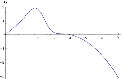
In Fig. 1 a plot of is shown. The zeros of correspond to de Sitter solutions. One can see that the only non-trivial zero is the de Sitter point of Eq. (V.22), and here the function crosses the -axis up-down, according to the instability of such solution (since , we get <0). This means that the inflationary de Sitter point corresponds to a maximum of the theory (without matter/radiation). The system gives rise to the de Sitter solution where the universe expands in an accelerating way but, suddenly, it exits from inflation and tends towards the minimal attractor at , unless the theory develops a singularity solutions for . In such case, the model could exit from inflation and move in the wrong direction, where the curvature would grow up and diverge, and a singularity would appear. In the next section we will recall some important facts about singularities, which will be considered in the context of exponential gravity.
VI Finite-time future singularities
In general, future singularities appear when the Hubble parameter has the form
| (VI.1) |
where and are positive constants, and , because it should correspond to an expanding universe. Here is a positive constant or a negative non-integer number, so that, when is close to , or some derivatives of , and therefore the curvature, become singular.
Note that such a choice of the Hubble parameter corresponds to an accelerated universe, because on the singular solution of Eq. (VI.1) it is easy to see that the strong energy condition () is always violated when , or for small values of when . What means that, in any case, a singularity could emerge at the final evolution stage of an accelerating universe.
The finite-time future singularities can be classified as follows [11]:
-
•
Type I (Big Rip): for , , and . It corresponds to and .
-
•
Type II (sudden): for , , and . It corresponds to .
-
•
Type III: for , , and . It corresponds to .
-
•
Type IV: for , , , and higher derivatives of diverge. The case in which and/or tend to finite values is also included. It corresponds to but is not any integer number.
Here, and are positive constants.
It is easy to see that in the case of Type I and Type III singularities we have . Those types are the most dangerous in the cosmological scenario. On the other hand, also the soft Type II and Type IV () singularities may cause various problems related , for instance, to the description of stellar astrophysics.
VI.1 Singularities in exponential gravity
Let us now consider the exponential model of Eq. (V.1), but avoiding the last term, . When , we have , , while the high-order derivatives of tend to zero in an exponential way. This means that in Eq. (II.22), by neglecting the matter contribution, tends to a constant on the singular solution of Eq. (VI.1) with (namely, ). For this reason, neither Type I nor Type III singularities, where has to diverge, can appear in exponential gravity. However, a model of this kind, which mimics the cosmological constant in the high-curvature regime, can be affected by Type II or IV singularities.
Regarding Type II singularities, we have to consider the behavior of the model when is negative, which is very different from the case of positive values of the curvature. This is the reason why this kind of singularities does not appear: when , of Eq. (II.22) exponentially diverge, and the sudden singularity, where has to tend to a constant, cannot be realized.
Also Type IV singularities are not realized: when , , and it is easy to see that of Eq. (II.22) behaves as , and it is larger than (), when . For this reason, Eq. (II.20) is inconsistent with Type IV singularities. The argument is valid also if we consider the more general case where and tends to the positive constant in the asymptotic singular limit: also in this situation approaches a constant like , while the time dependent part of behaves as .
Consider now adding back the term . This becomes relevant just when , so that it can produce Type I or III singularities, only. However, in Ref. [13] it is explicitly demonstrated that the model is protected against singularities of this kind if .
Thus, we have found our theory to be free from singularities. In particular, when our model is approximated as
| (VI.2) |
Type I or III singularities do not occur. When inflation ends, the model moves to the attractor de Sitter point. In this way, the small curvature regime arises, the first term of Eq. (V.1) becomes dominant and the physics of the CDM model are reproduced.
VII Dark energy epoch
We will now be interested in the cosmological evolution of the dark energy density in the case of the two-step model of Eq. (V.1), near the late-time acceleration era describing the current universe. We assume the spatially-flat FRW metric of Eq. (II.18). Let us follow the method first suggested in Ref. [16] and more recently used in Ref. [20].
To this end, we introduce the variable
| (VII.1) |
Here, is the energy density of matter at present time, is the mass scale
| (VII.2) |
and is defined as
| (VII.3) |
where is the energy density of radiation at present (the contribution from radiation is also taken into consideration).
The EoS-parameter for dark energy is
| (VII.4) |
By combining Eq. (II.20) with Eq. (II.19) and using Eq. (VII.1), one gets
| (VII.5) |
where
| (VII.6) |
| (VII.7) |
| (VII.8) |
and thus, we have
| (VII.9) |
The parameters of Eq. (V.1) are chosen as follows:
| (VII.10) |
Eq. (VII.5) can be solved in a numerical way, in the range of (matter era/current acceleration). is then found as a function of the red shift ,
| (VII.11) |
In solving Eq. (VII.5) numerically we have taken the following initial conditions at
| (VII.12) |
which correspond to the ones of the CDM model. This choice obeys to the fact that in the high red shift regime the exponential model is very close to the CDM Model. The values of have been chosen so that , assuming . We have , , for , , , respectively. In setting the parameters, we have used the last results of the MAP, BAO and SN surveys [23].
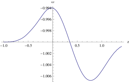
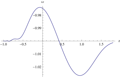
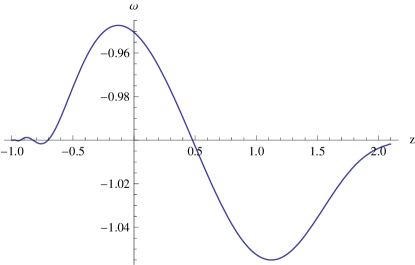
Using Eq. (VII.4), one derives from . In Figs. 2, 3 and 4, we plot as a function of the redshift for , , , respectively. Note that is very close to minus one. In the present universe (), one has , , for , , . The smaller is, our model becomes more indistinguishable from the CDM model, where .
We can also extrapolate the behavior of the density parameter of dark energy, ,
| (VII.13) |
Plots of as a function of the redshift for , , , are shown in Figs. 5, 6 and 7. For the present universe (), one has , , for , , , respectively.
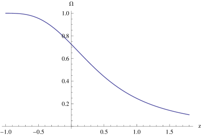
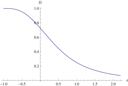

The data are in accordance with the last and very accurate observations of our present universe, where:
| (VII.14) |
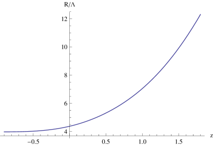
As last point, we want to analyze the behavior of the Ricci scalar in Eq. (VII.9) for , , . Results are shown in Figs. 8, 9 and 10. We clearly see that the transition crossing the phantom divide does not cause any serious problem to the accuracy of the cosmological evolution arising from our model. In particular, tends to , which is an effective cosmological constant (note that is small and we are close to the value of the CDM model, where ). As a consequence, the de Sitter solution is a final attractor of our system and describes an eternal accelerating expansion.


VIII Asymptotic behavior
As a last issue, we will analyze the solutions of our model when is very large in comparison with the de Sitter curvature . This means that Eq. (V.1) can be approximated by
| (VIII.1) |
which is proved by the fact that and, by setting , one has . In order to check for solutions, we use Eq. (II.22) and verify Eq. (II.20). A class of asymptotic solutions of the model of Eq. (VIII.1) at the limit is
| (VIII.2) |
where is a large positive constant and a positive parameter so that or . It follows from Eq. (II.19),
| (VIII.3) |
Eq. (II.22) gets
| (VIII.4) |
Here, is a positive constant and Eq. (II.20), in the limit , is perfectly consistent. This result shows that in the limit the model exhibits a past singularity, which could be identified with the Big Bang one. It is important to stress that this kind of solution is disconnected from the de Sitter inflationary solution, where the term is of the same order of and is therefore not negligible as in Eq. (VIII.1). We may assume that, just after the Big Bang, a Planck epoch takes over where physics is not described by GR and where quantum gravity effects are dominant. When the universe exits from the Planck epoch, its curvature is bound to be the characteristic curvature of inflation and the de Sitter solution takes over.
IX On the stability of de Sitter space and a realistic model without singularities
We here investigate in more detail the stability of the de Sitter solution (or its absence) and construct another model which does not generate any singularity. The de Sitter condition (II.11) can be rewritten as
| (IX.1) |
Let be a solution of (IX.1). Then has the form
| (IX.2) |
Here, is a constant, which should be positive if we require . We now assume that is an integer bigger or equal than : . Assume the function does not vanish at , . Since , one finds
| (IX.3) |
which tells us that in (II.15) vanishes. Therefore, a more detailed investigation is necessary in order to check stability. Using the expression of ,
| (IX.4) |
one can investigate the sign of in the region . Note that the Eq. (II.15) is not used since this expression is only valid at the point . Hence, we get
| (IX.5) |
Eq. (IX.5) indicates that, when is an even integer, the de Sitter solution is stable provided but it is unstable if . On the other hand, when is an odd integer, the de Sitter solution is always unstable. Note, however, that when , we find if , but if . Therefore when , becomes small but when , becomes large. The stability condition can thus be used to get realistic (unstable) de Sitter inflation for a specific gravity.
The following model, instead of (V.1), is considered (compare with [24]),
| (IX.6) |
Here is assumed to be an odd integer . We also assume that , , and are positive constants and that satisfies the condition . We choose to be small enough. When , we find and therefore the model (IV.1) is reproduced. When , behaves as in (IX.2), with
| (IX.7) |
Since and it is assumed that , we find
| (IX.8) |
and, therefore, there exists a de Sitter solution and the curvature always becomes smaller, slowly decreasing from the de Sitter point. Therefore, no future singularity is generated. When , behaves as
| (IX.9) |
Since , the singularity cannot emerge. Using the same numerical techniques as in the above sections, one can numerically fit this non-singular model with actual observable data coming from the dark energy epoch.
X Discussion
In summary, we have investigated in this paper some models corresponding to the quite simple exponential theory of modified gravity which are able to explain the early- and late-time universe accelerations in a unified way. The viability conditions of the models have been carefully investigated and it has been demonstrated that the theory quite naturally complies with the local tests as well as with the observational bounds. Moreover, the inflationary era has been proven to be unstable and graceful exit from inflation has been established. A numerical investigation of the dark energy epoch shows that the theory is basically non-distinguishable from the latest observational predictions of the standard CDM model in this range. Special attention has been paid in the paper to the occurrence of finite-time future singularities in the theory under consideration. It has been shown that it is indeed protected against the appearance of such singularities. Moreover, its evolution turns out to be asymptotically de Sitter (it has a late-time de Sitter universe as an attractor of the system). Hence, the future of our universe, according to such modified gravity, is eternal acceleration. We have also demonstrated that slight modifications of the theory may lead to other non-singular exponential gravities with similar predictions, what points towards a sort of stable class of well-behaved theories.
Very nice properties of exponential gravity are its extreme analytic simplicity, as well as the noted singularity avoidance. In this respect, the theory considered seems to be a very natural candidate for the study of cosmological perturbations and structure formation, which are among the most basic issues of evolutional cosmology. However, the theory remains in the class of higher-derivative gravities, which is not yet well understood, even concerning its canonical formulation [25]. In this respect, the covariant perturbation theory developed in [26] could presumably be applied for such investigation. This will be pursued elsewhere.
Acknowledgments
We are grateful to G. Cognola for his participation at the early stages of this work. This research has been supported in part by the INFN (Trento)-CSIC (Barcelona) exchange project 2010-2011, by MICINN (Spain) project FIS2006-02842, by CPAN Consolider Ingenio Project and AGAUR (Catalonia) 2009SGR-994 (EE and SDO), and by the Global COE Program of Nagoya University (G07) provided by the Ministry of Education, Culture, Sports, Science & Technology of Japan and the JSPS Grant-in-Aid for Scientific Research (S) # 22224003 (SN).
Appendix A The Einstein frame
gravity may be rewritten in scalar-tensor or Einstein frame form. In this case, one can present the Jordan frame action of modified gravity of Eq. (II.1) by introducing a scalar field which couples to the curvature. Of course, this is not exactly a physically-equivalent formulation, as explained in Ref. [27]. However, Einstein frame formulation may be used for getting some of the intermediate results in a simpler form (especially, when matter is not accounted for).
Let us introduce the field into Eq. (II.1):
| (I.1) |
Here “” means “Jordan frame”. By making the variation of the action with respect to , we have . The scalar field is defined as
| (I.2) |
Consider now the following conformal transformation of the metric,
| (I.3) |
for which Eq. (I.1) is invariant. By using Eq. (I.3), we get the Einstein frame () action of the scalar field :
| (I.4) |
where
| (I.5) |
is the solution of Eq. (I.2):
| (I.6) |
In order to pass to the scalar-tensor theory, we need the explicit form of the potential . In principle, the result of Eq. (I.6) will be in the form of a complicated transcendental function. However, in exponential gravity the calculation simplifies a lot.
References
- [1] I.L. Buchbinder, S.D. Odintsov and I.L. Shapiro, Effective Action in Quantum Gravity (IOP, Bristol, 1992).
- [2] G. Cognola, E. Elizalde, S. Nojiri, S.D. Odintsov and S. Zerbini, Phys. Rev. D 73, 084007 (2006); hep-th/0601008.
- [3] S. Nojiri and S. D. Odintsov, Phys. Lett. B 576, 5 (2003) [arXiv:hep-th/0307071].
- [4] S. Nojiri and S. D. Odintsov, arXiv:1011.0544 [gr-qc]; eConf C0602061, 06 (2006), Int. J. Geom. Meth. Mod. Phys. 4, 115, hep-th/0601213 (2007).
-
[5]
S. Capozziello and M. Francaviglia,
Gen. Rel. Grav. 40, 357 (2008)
[arXiv:0706.1146 [astro-ph]];
S. Capozziello, M. De Laurentis and V. Faraoni, arXiv:0909.4672 [gr-qc]. - [6] S. Nojiri and S. D. Odintsov, Phys. Rev. D 68, 123512 (2003) [arXiv:hep-th/0307288].
- [7] L. Sebastiani, S. Zerbini, [arXiv:1012.5230 [gr-qc]].
-
[8]
A. D. Dolgov and M. Kawasaki,
Phys. Lett. B 573, 1 (2003)
[arXiv:astro-ph/0307285];
V. Faraoni, Phys. Rev. D 74 (2006) 104017 [arXiv:astro-ph/0610734]. - [9] S. Nojiri and S. D. Odintsov, Phys. Lett. B 652, 343 (2007) [arXiv:0706.1378 [hep-th]].
-
[10]
R. R. Caldwell, M. Kamionkowski and N. N. Weinberg,
Phys. Rev. Lett. 91, 071301 (2003)
[arXiv:astro-ph/0302506];
B. McInnes, JHEP 0208 (2002) 029 [arXiv:hep-th/0112066];
S. Nojiri and S. D. Odintsov, Phys. Lett. B 562, 147 (2003) [arXiv:hep-th/0303117];
E. Elizalde, S. Nojiri and S. D. Odintsov, Phys. Rev. D 70, 043539 (2004) [arXiv:hep-th/0405034];
V. Faraoni, Int. J. Mod. Phys. D 11, 471 (2002) [arXiv:astro-ph/0110067];
P. F. Gonzalez-Diaz, Phys. Lett. B 586, 1 (2004) [arXiv:astro-ph/0312579];
C. Csaki, N. Kaloper and J. Terning, Annals Phys. 317, 410 (2005) [arXiv:astro-ph/0409596];
P. X. Wu and H. W. Yu, Nucl. Phys. B 727, 355 (2005) [arXiv:astro-ph/0407424];
S. Nesseris and L. Perivolaropoulos, Phys. Rev. D 70, 123529 (2004) [arXiv:astro-ph/0410309];
M. Sami and A. Toporensky, Mod. Phys. Lett. A 19, 1509 (2004) [arXiv:gr-qc/0312009];
H. Stefancic, Phys. Lett. B 586, 5 (2004) [arXiv:astro-ph/0310904];
L. P. Chimento and R. Lazkoz, Mod. Phys. Lett. A 19, 2479 (2004) [arXiv:gr-qc/0405020];
E. Babichev, V. Dokuchaev and Yu. Eroshenko, Class. Quant. Grav. 22, 143 (2005) [arXiv:astro-ph/0407190];
X. F. Zhang, H. Li, Y. S. Piao and X. M. Zhang, Mod. Phys. Lett. A 21, 231 (2006) [arXiv:astro-ph/0501652];
M. P. Dabrowski and T. Stachowiak, Annals Phys. 321, 771 (2006) [arXiv:hep-th/0411199];
I. Y. Aref’eva, A. S. Koshelev and S. Y. Vernov, Phys. Rev. D 72, 064017 (2005) [arXiv:astro-ph/0507067];
E. M. Barboza and N. A. Lemos, Gen. Rel. Grav. 38, 1609 (2006) [arXiv:gr-qc/0606084]. - [11] S. Nojiri, S. D. Odintsov and S. Tsujikawa, Phys. Rev. D 71, 063004 (2005); [arXiv:hep-th/0501025].
-
[12]
K. Bamba, S. Nojiri and S. D. Odintsov,
JCAP 0810, 045 (2008)
[arXiv:0807.2575 [hep-th]];
S. Nojiri and S. D. Odintsov, Phys. Rev. D 78, 046006 (2008) [arXiv:0804.3519 [hep-th]]; AIP Conf. Proc. 1241, 1094 (2010) [arXiv:0910.1464 [hep-th]]. - [13] K. Bamba, S. D. Odintsov, L. Sebastiani and S. Zerbini, Eur. Phys. J. C 67, 295 (2010) [arXiv:0911.4390 [hep-th]].
-
[14]
T. Kobayashi and K. I. Maeda,
Phys. Rev. D 78, 064019 (2008)
[arXiv:0807.2503 [astro-ph]];
S. Capozziello, M. De Laurentis, S. Nojiri and S. D. Odintsov, Phys. Rev. D 79, 124007 (2009) [arXiv:0903.2753 [hep-th]]. - [15] M. C. B. Abdalla, S. Nojiri and S. D. Odintsov, Class. Quant. Grav. 22, L35 (2005) [arXiv:hep-th/0409177].
- [16] W. Hu and I. Sawicki, Phys. Rev. D 76, 064004 (2007) [arXiv:0705.1158 [astro-ph]].
- [17] S. A. Appleby and R. A. Battye, Phys. Lett. B 654, 7 (2007) [arXiv:0705.3199 [astro-ph]].
- [18] G. Cognola, E. Elizalde, S. Nojiri, S. D. Odintsov, L. Sebastiani and S. Zerbini, Phys. Rev. D 77, 046009 (2008) [arXiv:0712.4017 [hep-th]].
- [19] E. V. Linder, Phys. Rev. D 80, 123528 (2009) [arXiv:0905.2962 [astro-ph.CO]].
- [20] K. Bamba, C. Q. Geng and C. C. Lee, JCAP 1008, 021 (2010) [arXiv:1005.4574 [astro-ph.CO]].
- [21] D. S. Gorbunov and A. G. Panin, arXiv:1009.2448 [hep-ph].
- [22] L. Yang, C. C. Lee, L. W. Luo and C. Q. Geng, arXiv:1010.2058 [astro-ph.CO].
- [23] E. Komatsu et al. [WMAP Collaboration], Astrophys. J. Suppl. 180, 330 (2009) [arXiv:0803.0547 [astro-ph]].
- [24] S. Nojiri and S. D. Odintsov, arXiv:1008.4275 [hep-th].
- [25] R. P. Woodard, Lect. Notes Phys. 720, 403 (2007) [arXiv:astro-ph/0601672].
- [26] S. Carloni, P. K. S. Dunsby and A. Troisi, Phys. Rev. D 77, 024024 (2008) [arXiv:0707.0106 [gr-qc]].
- [27] S. Capozziello, S. Nojiri, S. D. Odintsov and A. Troisi, Phys. Lett. B 639, 135 (2006) [arXiv:astro-ph/0604431].