Cross-Phase Modulation and Population Redistribution in a Periodic Tripod Medium

Abstract

The cross-Kerr effect is studied for two weak beams, probe and trigger, propagating in an atomic medium in a tripod configuration, dressed by a strong standing wave coupling beam in a regime of electromagnetically induced transparency. The nonlinear phase shifts for both transmitted and reflected probe beams induced by the trigger’s presence are found to depend on the probe detuning, the control beams intensity, the relaxation rates and, in particular, on the redistribution of the population among the atomic levels. Such a quantitative analysis indicates that the transmitted and reflected probe beam components and their respective phase shifts can be easily controlled and optimized.

I Introduction

All-optical nonlinearities at low light levels are instrumental to the optical implementation of quantum information processing systems. Large nonlinearities can be achieved when the light-matter interaction is resonant, in which case however absorption typically plays a detrimental role. A great deal of attention has thus been devoted to a variety of schemes based on the regime of electromagnetically induced transparency (EIT) fleischhauer in which this counterbalance can be overcome. In a typical EIT configuration, a strong control field, coupling two unpopulated levels of a $\Lambda$ system, creates a transparency window for a weak probe beam. This basic scheme was extended by including additional atomic levels coupled by laser or microwave fields in the double-$\Lambda$ my04 , tripod paspalakis ; mazets ; my07 , $N$ kang ; wilson or inverted-$Y$ joshi configurations, just to name a few. Under EIT-like conditions the weak interaction between two photons (or weak classical pulses) may become largely enhanced. In particular, very large cross nonlinear effects have been predicted leading to new types of polarization phase gates in an optically dressed medium in the $M$ ottaviani , tripod rebic ; petr or inverted-$Y$ joshi2 configuration. Relevant experimental work has very recently been reported in Ref. yang . In these instances, a significant change of the phase of one of the propagating pulses is achieved due to the cross-Kerr effect induced by the other pulse. Analogous effects have recently been studied, both theoretically and experimentally, for an inverted-$Y$ system kou , as well as for a four-level $N$-type lo and five-level system wang . Important developments concern also the dynamic control of the process leading, e.g., to light slowdown, storage and release liu ; matsko . These results are expected to pave the way towards constructing all-optical logical devices.

Unlike most typical EIT configurations employing a running wave coupling field, using a control standing wave coupling beam opens the possibility of creating an all-optically tunable Bragg mirror. In such a novel kind of dynamically tunable metamaterial andre ; my09 an incoming probe light encounters a spatially periodic optical structure and is subject to Bragg scattering. For specific frequency ranges transmission and stop bands appear, the properties of which can be steered by a proper choice of the control field. The field-induced dispersion of the medium and the transmission and reflection spectra have been analyzed, e.g., in Refs. andre ; my09 ; myNowa , including the case of a quasi-standing wave coupling field artoni2 . It was also possible to stop and store a pulse inside the medium, and then retrieve it in the form of a stationary light pulse which could not leave the medium due to the standing wave character of the releasing control beam andre ; bajcsy . It has also been shown that high nonlinearities can be achieved for stored light pulses newchen . An all-optical dynamic cavity for the confinement of light pulses based on standing wave EIT Bragg mirrors has recently been proposed wucav .

Very recently, we have pointed out that in the presence of a trigger beam in a tripod configuration, a probe partially reflected from the periodic structure induced by a strong standing wave EIT coupling field undergoes large cross-Kerr nonlinear phase shifts. Such a novel configuration is specifically apt for developing a phase-tunable beam splitter in which both the amplitudes and the phases of the trasmitted and reflected beam can be controlled. We have given some illustrative results valid in a narrow range of frequencies owing to the restrictive assumption that the atomic population is symmetrically distributed between the two lower levels that are coupled with the upper level respectively by the probe and trigger pulses myScripta . Here, we provide a comprehensive theoretical study of the problem, including a proper treatment of the population redistribution. The latter point turns out to be crucial to extend the range of possible probe detunings and, thus, optimize the control possibilities. Our approach combines analytical methodologies used to describe propagation effects in both nonlinear and spatially periodic media, and allow us to numerically examine the phase shifts of the reflected and transmitted probe field induced by the trigger’s presence over a wide range of probe detunings as well as their dependence on various parameters characterizing both the atomic medium and the three laser fields. Our results indicate that the tripod standing wave EIT configuration makes control over the cross-Kerr effect more versatile than for a running wave EIT configuration rebic ; petr in which no reflected beam appears.

The paper is organized as follows. In Section II, we present the basic theoretical approach to calculate the cross-Kerr effect in a medium additionally dressed by a quasi-standing wave EIT coupling field, based on expanding the medium susceptibility into a power series with respect to the probe and trigger fields and into a Fourier series appropriate to the spatial periodicity imposed by the coupling field. In Appendix A we derive in detail the formulae for the susceptibility’s expansion coefficients, while in Appendix B we present the way to evaluate the population redistribution. In Section III, we present and discuss the numerical results for the trigger induced nonlinear phase shifts of the reflected and transmited probe fields as functions of the probe detuning for various combinations of control field intensities, relaxation rates and sample length. Finally, we draw our conclusions.

II Theory

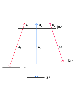
Figure 1: (color online). The level and coupling scheme of the tripod configuration.

We consider a tripod system driven by a strong control field ($\mathcal{E}_{c}$) coupling the ground level $2$ and the upper level $0$, and by two weaker laser fields called probe ($\mathcal{E}_{p}$) and trigger ($\mathcal{E}_{t}$), coupling $0$ with $1$ and $3$, respectively, as shown in Fig. 1. We express the fields through their complex amplitudes $\epsilon_{p,c,t}$ slowly varying in time:

$$\mathcal{E}_{p,c,t}=\epsilon_{p,c,t}e^{-i\omega_{1,2,3}t}+\epsilon_{p,c,t}^{*}e^{i\omega_{1,2,3}t}.$$

Each of the couplings is detuned by $\delta_{j}\equiv E_{j}+\hbar\omega_{j}-E_{0}$, $j=1,2,3$. Here $E_{j}$ stands for the energy of the state $j$ and $\omega_{j}$ denotes the frequency of the $j$-th field.

All the fields propagate along the $z$ axis. In general the control wave is allowed to have two counter-propagating components of arbitrary ratio. In the case of a running control wave, the component antiparallel to the incoming probe and trigger fields is zero. In the case of a perfect standing wave, both components are equal. Thus, the control field provides a spatial lattice of period $\frac{\pi}{k_{2}}$, $k_{2}$ being the field’s wave number. In the configuration proposed below $k_{2}$ may be slightly different from the probe and trigger fields’ wave vectors $k_{1,3}$, but that can be corrected by tilting both components of the control field by an angle $\theta$ with respect to the $z$-axis so that $\omega_{2}\cos\theta/c\approx k_{1,3}$ artoni2 .

Such a configuration can be realized in a cold gas of ⁸⁷Rb atoms. The states $1$ and $3$ may correspond, e.g., to Zeeman sublevels $|5S_{\frac{1}{2}},F=2,m=\{-1,1\}>$, state $2$ to $|5S_{\frac{1}{2}},F=1,m=1>$, and the upper state $0$ to the level $|5P_{\frac{3}{2}},F=1,m=0>$. The scheme could be used as a polarization phase gate, as was first proposed in Ref. rebic . Each of the two pulses interacts with the medium when it has the proper circular polarization: right for the probe and left for the trigger. When both pulses are properly polarized the nonlinear interaction between them gives rise to a cross-phase modulation.

The Bloch equations for the atom + field system in the rotating wave approximation read:

$$i\dot{\sigma}_{00} = \Omega_{p}\sigma_{10}+\Omega_{c}\sigma_{20}+\Omega_{t}\sigma_{30}-\Omega_{p}^{*}\sigma_{01}-\Omega_{c}^{*}\sigma_{02}-$$

$$- \Omega_{t}^{*}\sigma_{03}-i(\gamma_{11}+\gamma_{22}+\gamma_{33})\sigma_{00}$$

$$i\dot{\sigma}_{11} = \Omega_{p}^{*}\sigma_{01}-\Omega_{p}\sigma_{10}+i\gamma_{11}\sigma_{00}-i\gamma_{12}\sigma_{11}+i\gamma_{13}\sigma_{33}$$

$$i\dot{\sigma}_{22} = \Omega_{c}^{*}\sigma_{02}-\Omega_{c}\sigma_{20}+i\gamma_{22}\sigma_{00}+i\gamma_{12}\sigma_{11}+i\gamma_{23}\sigma_{33}$$

$$i\dot{\sigma}_{33} = \Omega_{t}^{*}\sigma_{03}-\Omega_{t}\sigma_{30}+i\gamma_{33}\sigma_{00}-i(\gamma_{13}+\gamma_{23})\sigma_{33}$$

$$i\dot{\sigma}_{10} = \Delta_{10}^{*}\sigma_{10}-\Omega_{p}^{*}(\sigma_{11}-\sigma_{00})-\Omega_{c}^{*}\sigma_{12}-\Omega_{t}^{*}\sigma_{13}$$

$$i\dot{\sigma}_{20} = \Delta_{20}^{*}\sigma_{20}-\Omega_{c}^{*}(\sigma_{22}-\sigma_{00})-\Omega_{p}^{*}\sigma_{21}-\Omega_{t}^{*}\sigma_{23}$$ (1)

$$i\dot{\sigma}_{30} = \Delta_{30}^{*}\sigma_{30}-\Omega_{t}^{*}(\sigma_{33}-\sigma_{00})-\Omega_{c}^{*}\sigma_{32}-\Omega_{p}^{*}\sigma_{31}$$

$$i\dot{\sigma}_{12} = \Delta_{12}^{*}\sigma_{12}+\Omega_{p}^{*}\sigma_{02}-\Omega_{c}\sigma_{10}$$

$$i\dot{\sigma}_{13} = \Delta_{13}^{*}\sigma_{13}+\Omega_{p}^{*}\sigma_{03}-\Omega_{t}\sigma_{10}$$

$$i\dot{\sigma}_{23} = \Delta_{23}^{*}\sigma_{23}+\Omega_{c}^{*}\sigma_{03}-\Omega_{t}\sigma_{20}$$

where $\sigma_{mm}=\varrho_{mm}$, $\sigma_{0j}=\varrho_{0j}e^{i\omega_{j}t}$, $\sigma_{jk}=\varrho_{jk}e^{-i(\omega_{j}-\omega_{k})t}$, and $\varrho$ is the density matrix of the atoms in the Schrödinger picture, $\Delta_{j0}=\delta_{j}+i\gamma_{j0}$, $\Delta_{jk}=\delta_{j}-\delta_{k}+i\gamma_{jk}$, $\gamma_{jk}=\gamma_{kj}$, $j,k=1,2,3$, $m=0,1,2,3$. The Rabi frequencies are defined by $\Omega_{p,c,t}=-\frac{d_{01,02,03}\epsilon_{p,c,t}}{\hbar}$, where $d_{0j}$ is the electric dipole moment matrix element.

The simplified model of relaxations adopted in the above equations takes into account spontaneous emission from the upper state $0$ to a lower state $k$, described by the relaxation rates $\gamma_{0k}$ and $\gamma_{kk}$ with $\gamma_{0k}=\frac{1}{2}(\gamma_{11}+\gamma_{22}+\gamma_{33})$, as well as deexcitation and decoherence between the lower levels $\gamma_{jk}$, $j\neq k=1,2,3$, due to atomic collisions. The relaxation rates for the coherences $\sigma_{jk}$, $j\neq k$, and those for the collision-induced population relaxations were taken equal for simplicity (cf. Ref. rebic ).

The propagation equation for the positive frequency part of the probe field, slowly varying in time, i.e. when $|\frac{\partial\epsilon_{p}}{\partial t}|<<\omega_{1}|\epsilon_{p}|$, reads in the Fourier picture, with the Fourier frequency variable identified with the probe detuning

$$\left[\frac{\partial^{2}}{\partial z^{2}}+\frac{1}{c^{2}}\left(\omega_{1}^{2}+2\omega_{1}\delta_{1}\right)\right]\epsilon_{p}(z,\delta_{1})=-\frac{\omega_{1}^{2}}{c^{2}}\chi_{p}(z,\delta_{1})\epsilon_{p}(z,\delta_{1}),$$ (2)

with the medium susceptibility for the probe given by

$$\chi_{p}=-\lim_{t\rightarrow\infty}\frac{N|d_{10}|^{2}}{\hbar\epsilon_{0}}\frac{\sigma_{01}}{\Omega_{p}},$$ (3)

where $N$ is the number of atoms per unit volume. The time limit means that we need to find the steady state solutions to the Bloch equations.

The assumption that the probe and trigger are weak with respect to the control field $|\Omega_{p}|^{2},|\Omega_{t}|^{2}<<|\Omega_{c}|^{2}$ allows us to expand the susceptibility into the Taylor series:

$$\chi_{p}\approx\chi_{p}^{(1)}+\chi_{pp}^{(3)}|\Omega_{p}|^{2}+\chi_{pt}^{(3)}|\Omega_{t}|^{2}.$$ (4)

The explicit form of the Taylor expansion coefficients can be found in Appendix A. The term $\chi_{p}^{(1)}$ corresponds to the linear susceptibility, while the third-order terms $\chi_{pp}^{(3)}$ and $\chi_{pt}^{(3)}$ represent the self- and cross-Kerr effect, respectively. The latter is of particular importance, as we are interested in the cross-phase modulation.

We now write the control field as:

$$\Omega_{c}=\Omega_{c}^{+}e^{ik_{2}z}+\Omega_{c}^{-}e^{-ik_{2}z},$$ (5)

where $\Omega_{c}^{\pm}$ of constant values are its forward and backward propagating parts. As the field is periodic in space, so are the medium optical properties. Therefore we expand the susceptibilities for both probe and trigger into the Fourier series:

$$\chi_{p}=\sum_{n=-\infty}^{\infty}\left[\chi_{p,2n}^{(1)}+\chi_{pt,2n}^{(3)}|\Omega_{t}|^{2}+\chi_{pp,2n}^{(3)}|\Omega_{p}|^{2}\right]e^{2ink_{2}z}.$$ (6)

The pulses propagating in a periodic medium acquire their reflected components. In the two-mode approximation (for details see artoni2 ; my09 ) we write:

$$\Omega_{p,t}=\Omega^{+}_{p,t}e^{ik_{2}z}+\Omega^{-}_{p,t}e^{-ik_{2}z},$$ (7)

where $\Omega^{\pm}_{p,t}$ are slowly varying in space.

We now insert Eqs. (6,7) into Eq. (2) and drop terms rapidly oscillating in space. To write the propagation equations in the final form we make use of the relation $k_{2}=\frac{\omega_{2}}{c}$ and set $\omega_{2}=\omega_{1}+\Delta\omega_{1}$. For the probe we find:

$$\left(i\frac{\partial}{\partial z}+\frac{\delta_{1}}{c}-\frac{\Delta\omega_{1}}{c}\right)\Omega_{p}^{+} = -\frac{\omega_{1}}{2c}\left(X\Omega_{p}^{+}+Y\Omega_{p}^{-}\right),$$ (8)

$$\left(-i\frac{\partial}{\partial z}+\frac{\delta_{1}}{c}-\frac{\Delta\omega_{1}}{c}\right)\Omega_{p}^{-} = -\frac{\omega_{1}}{2c}\left(X\Omega_{p}^{-}+Z\Omega_{p}^{+}\right),$$ (9)

where

$$X = \chi_{p,0}^{(1)}+\chi_{pt,0}^{(3)}S_{t}^{2}+\chi_{pp,0}^{(3)}S_{p}^{2}+$$

$$+ 2\chi_{pt,2}^{(3)}\Re(\Omega_{t}^{+}{\Omega_{t}^{-*}})+2\chi_{pp,2}^{(3)}\Re(\Omega_{p}^{+}{\Omega_{p}^{-*}}),$$

$$Y = \chi_{p,2}^{(1)}+\chi_{pt,2}^{(3)}S_{t}^{2}+\chi_{pp,2}^{(3)}S_{p}^{2}+\chi_{pt,0}^{(3)}\Omega_{t}^{+}{\Omega_{t}^{-*}}+$$

$$+ \chi_{pt,4}^{(3)}\Omega_{t}^{-}{\Omega_{t}^{+*}}+\chi_{pp,0}^{(3)}\Omega_{p}^{+}{\Omega_{p}^{-*}}+\chi_{pp,4}^{(3)}\Omega_{p}^{-}{\Omega_{p}^{+*}},$$

$$Z = \chi_{p,2}^{(1)}+\chi_{pt,2}^{(3)}S_{t}^{2}+\chi_{pp,2}^{(3)}S_{p}^{2}+\chi_{pt,0}^{(3)}\Omega_{t}^{+*}{\Omega_{t}^{-}}+$$

$$+ \chi_{pt,4}^{(3)}\Omega_{t}^{-*}{\Omega_{t}^{+}}+\chi_{pp,0}^{(3)}\Omega_{p}^{+*}{\Omega_{p}^{-}}+\chi_{pp,4}^{(3)}\Omega_{p}^{-*}{\Omega_{p}^{+}},$$

with $S_{p,t}^{2}\equiv|\Omega_{p,t}^{+}|^{2}+|\Omega_{p,t}^{-}|^{2}$. The trigger equations are obtained by interchanging the indices $\{p,1\}\leftrightarrow\{t,3\}$. Explicit formulae for the susceptibilities Fourier components as well as their detailed deriviation can be found in Appendix A.

As we will change the probe detuning $\delta_{1}$ in a wide range while keeping the trigger detuning $\delta_{3}$ constant, we introduce an asymmetry in the populations $\sigma_{11}$ and $\sigma_{33}$ even for $\Omega_{p}=\Omega_{t}$. Additionally, the symmetry may be spoiled by the fact that $E_{1}$ (the energy of the state $1$) is slightly smaller than $E_{3}$, and in a cold medium transitions from $3$ to $1$ are possible while those from $1$ to $3$ are not. In previous works (see Refs. rebic ; myScripta ) the probe and trigger fields were only allowed detunings such that $\delta_{1}\approx\delta_{3}$. In that case the stationary population distribution was assumed to be $\sigma_{11}=\sigma_{33}=\frac{1}{2}$. Such an approach is simple, but it is well justified only in the resonance region of frequencies. As we show in the section III, for a wider range of pulse detunings it is necessary to make a better estimation of the population distribution. In Appendix B we present the way to evaluate the populations in the case of a quasi-standing coupling beam ($\Omega_{c}^{+}\neq\Omega_{c}^{-}$, as in Ref.artoni2 ).

III Results and discussion

In this section we present numerical results illustrating the cross-Kerr effect in our system and its dependence on the system parameters. In particular, we discuss how the cross-phase modulation is affected by the population redistribution.

We have solved the propagation equations (8,9) with the boundary conditions corresponding to both probe and trigger originally propagating towards positive $z$:

$$\Omega_{p,t}^{+}(z=0,\delta_{1,3}) = {\Omega_{0}}_{p,t},$$ (10)

$$\Omega_{p,t}^{-}(z=L,\delta_{1,3}) = 0,$$

where ${\Omega_{0}}_{p,t}$ describes the amplitude of the incoming probe/trigger pulse and $L$ is the sample length. We have used the susceptibilities’ Fourier components as presented in Appendix A. The level populations have been evaluated as described in Appendix B, using the initial amplitudes of the probe and trigger fields as input data. Note that, strictly speaking, the populations in the standing wave case are also modulated in space. However, as discussed below, the latter effect should not play a very important role in the case of an quasi-standing wave.

The equations are solved iteratively until self-consistency is achieved, alternately for the probe and trigger, with the susceptibilities calculated using the fields obtained in the preceding step. In the first iteration for the probe the initial constant value of the trigger has been used. The numerical task in each step is thus solving a linear equation. We find two independent solutions with one-point boundary conditions and combine them to obtain the solution with the proper two-point boundary conditions given by Eqs. (10).

The transmission and reflection coefficients for the probe and trigger beams are defined by:

$$T_{p,t}(\delta_{1,3}) = \left|\frac{\Omega_{p,t}^{+}(L,\delta_{1,3})}{{\Omega_{0}}_{p,t}}\right|^{2},$$ (11)

$$R_{p,t}(\delta_{1,3}) = \left|\frac{\Omega_{p,t}^{-}(0,\delta_{1,3})}{{\Omega_{0}}_{p,t}}\right|^{2},$$

while the phases of the transmitted and reflected fields are given by:

$$\varphi^{+}_{p,t}(\delta_{1,3}) = \arg(\Omega_{p,t}^{+}(L,\delta_{1,3})),$$ (12)

$$\varphi^{-}_{p,t}(\delta_{1,3}) = \arg(\Omega_{p,t}^{-}(0,\delta_{1,3})).$$

Unless otherwise specified, we use the following set of input data which are of order of those of typical atomic systems: $\Omega_{c}^{+}=4$ MHz, $\Omega_{c}^{-}=2$ MHz, $\Omega_{p0}=\Omega_{t0}=0.67$ MHz, $\gamma_{10,20,30}=0.67$ MHz, $\gamma_{12,32,13}=6.67\times 10^{-4}$ MHz, $\gamma_{11,22,33}=0.44$ MHz, $\delta_{2}=6.67$ MHz, $\delta_{3}=1.002\times 6.67$ MHz, $L=1.06$ mm, $d_{10}=d_{30}=8\times 10^{-30}$ C^.m, $N=1.3\times 10^{13}$ cm^-3. Our choosing a quasi-standing wave is connected with the fact that for a perfect one the steady state population in the node regions is trapped in the state $2$ due to relaxation effects and the medium becomes transparent to both probe and trigger. Therefore, it is reasonable to only consider the cases in which the control field at the quasinodes is still strong enough to pump the population from the level $2$.

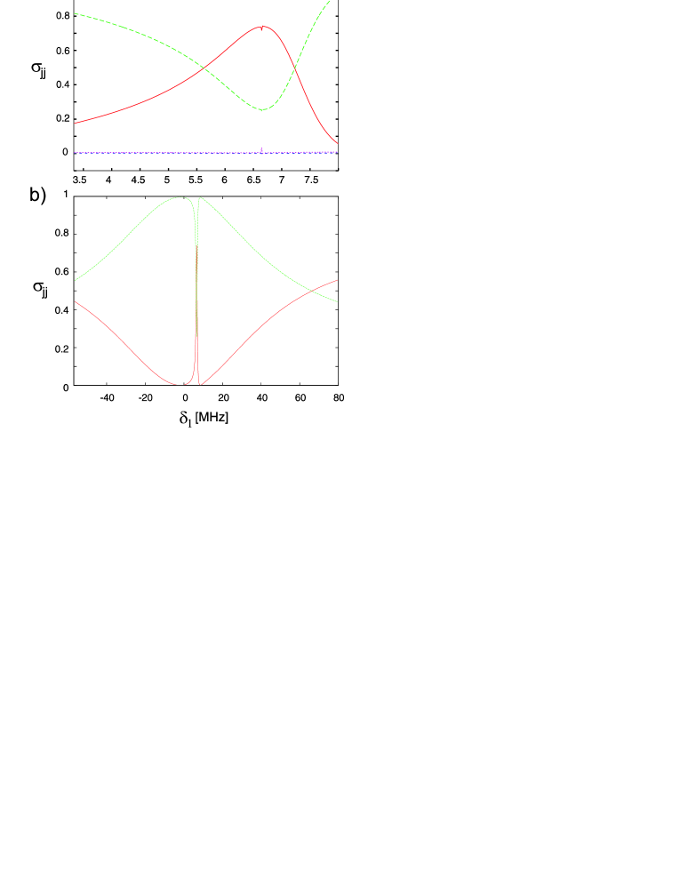
Figure 2: (color online). The population distribution in the case of trigger present: $\sigma_{11}$ - solid red line, $\sigma_{33}$ - dashed green line, $\sigma_{00}$ - short-dashed blue line, $\sigma_{22}$ - dotted violet line, for a narrow (a) and wide (b) frequency range. The populations $\sigma_{00}$ and $\sigma_{22}$ are negligible and thus not shown in the case (b).

We first calculate the corrected values of the populations which are shown in Fig. 2 in a narrow (plot (a)) and wide (plot (b)) ranges of the probe detunings. Note that the populations $\sigma_{11}$ and $\sigma_{33}$ may significantly differ from $\frac{1}{2}$. They may vary rapidly within the transparency window and the maximum value of $\sigma_{33}$ may be close to unity which apparently occurs when the frequency of the probe suits the energy interval between $E_{0}$ and the energy of one of the lower states dressed by $\Omega_{c}$ and $\Omega_{t}$. Between the maxima there is a deep minimum of $\sigma_{33}$ due to the population trapping in the state $1$. The populations of $\sigma_{00}$ and $\sigma_{22}$ are negligible, which is consistent with our assumption.

If there are no relaxations in the system, then the steady state solution for the no-trigger case is trivial: $\sigma_{33}=1$, $\sigma_{11}=\sigma_{00}=\sigma_{22}=0$ due to spontaneous emission from the upper level to all the lower levels. There is no mechanism yet pumping the population out from $3$. The nonnegligible relaxations provide such a mechanism and the plot illustrating the $\sigma_{33}$ dependence on the probe detuning is of a similar shape as in the trigger-present case (not shown).

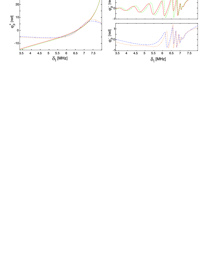
Figure 3: (color online). Probe field’s phase shift $\varphi_{p}(\delta_{1})$ vs the probe detuning in the presence (solid red) or absence (dashed green) of the trigger for balanced population distributions $\sigma_{11}=\sigma_{33}=0.5$. Phase shift in the presence (dash-dotted blue) or absence (dotted orange) of the trigger when instead the population distribution is given by Eqs. (B.3). The frame (a) refers to the transmitted probe phase shift ($\varphi_{p}^{+}(\delta_{1})$) acquired in the running wave configuration, whereas the frame (b) refers to the reflected probe phase shift ($\varphi_{p}^{-}(\delta_{1})$) acquired in the quasi-standing wave configuration.

The phase shifts for a running control field ($\Omega_{c}^{+}=4$ MHz, $\Omega_{c}^{-}=0$, the other parameters unchanged) are shown in Fig. 3a. We compare the results for the transmitted probe beam in the cases of equal or corrected values of the populations $\sigma_{11}$ and $\sigma_{33}$ and for the trigger pulse present or absent. The values of the obtained phase shifts $\varphi_{p}^{+}(\delta_{1})$ differ significantly for the two approximations concerning the populations, except for three points: when the calculated population distribution is almost exact: $\sigma_{11}=\sigma_{33}\approx 0.5,\sigma_{22}=\sigma_{00}\approx 0$ and within the resonance region $\delta_{1}\approx\delta_{2}\approx\delta_{3}$. The trigger-induced (Kerr) phase shifts (the differences between the values given by pairs of curves) in the two cases are also different and there are frequency intervals in which the Kerr shifts are significantly larger in the case in which the populations have been calculated according to Eqs. (B.3). In this way the results of Ref. rebic can be generalized for a wider range of the probe detunings.

In Fig. 3b we make a similar comparison for a reflected beam in the case of a quasi - standing control field ($\Omega_{c}^{+}=4.19$ MHz, $\Omega_{c}^{-}=2$ MHz, the other parameters unchanged). Again taking into account the population redistribution (lower plot) caused a qualitative change of the behaviour of the phase shifts as well as of their differences (the Kerr shifts) compared with the case of equal populations. The results are in agreement at the same three points as before. However, at $\delta_{1}\approx\delta_{2}\approx\delta_{3}$, due to a numerical instability in the algorithm used to find the solutions of Eq. (B.3), the calculated density matrix is no longer positive definite and our results in this very narrow spectral region are unphysical (see the sharp spikes appearing in Fig. 2).

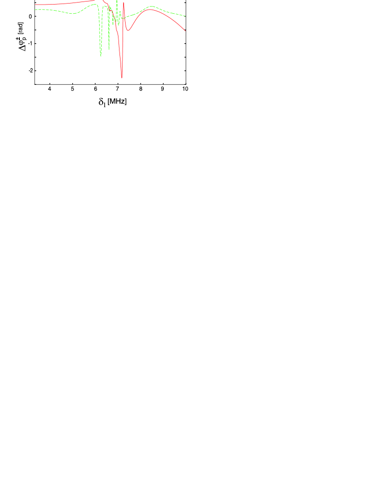
Figure 4: (color online). Trigger-induced probe phase shifts $\Delta\varphi^{\pm}_{p}$ as a function of the probe detuning for transmission (solid red) and reflection (dashed green). The population distribution is given by Eqs. (B.3) while all other parameters are as in Fig. 3b.

In Fig. 4 we show the cross-Kerr phase shifts $\Delta\varphi^{\pm}_{p}(\delta_{1})$ due to the trigger’s presence for both the transmitted and reflected probe beams defined as $\Delta\varphi^{\pm}_{p}=\varphi_{p}^{\pm}$(trigger on)$-\varphi_{p}^{\pm}$(trigger off). One can see that the shifts may be of order of one radian and there is a frequency range in which they do not change rapidly. The narrow minima or maxima in Fig. 4 correspond to the situation in which the phases $\varphi^{\pm}_{p}$ vary rapidly. The present results show how our system behaves as an all-optically controlled Kerr medium. In particular, it may serve as a tunable beam splitter for the probe beam in which the phases of the reflected and/or trasmitted beam are significantly affected by the trigger beam. For example, for detunings of $\delta_{1}\sim 5.5$ MHz or of $\delta_{1}\sim 6.4$ MHz at which both the transmission and reflection coefficients are large (see Fig. 6), the trigger induced phase shift of the trasmitted and reflected probe beams are both appreciable. On the contrary, for a detuning of $\delta_{1}\sim 6.25$ MHz at which both the transmission and reflection coefficients are considerable (see Fig. 6), while the trigger induced phase shift for the transmitted probe beam is significant, that of the reflected beam is negligible. This beam splitting action accompanied by a trigger induced phase shift of the reflected and/or transmitted probe components is a unique feature of the tripod standing wave EIT configuration with respect to others previously considered. Taking into account the redistribution of the population among the atomic levels is however crucial. If the redistribution were ignored the phase shifts could only be estimated within rather limited ranges of frequencies. In particular, while for $\delta_{1}\sim 5.5$ MHz the approximation $\sigma_{11}=\sigma_{33}=0.5$ is still reasonable as shown in Fig. 2, for $\delta_{1}\sim 6.4$ MHz or $\delta_{1}\sim 8.7$ MHz it fails. In the following, in order to illustrate the dependence of the Kerr effect on various parameters, we discuss several numerical results obtained over a large detuning range using the method here developed to calculate the population redistribution.

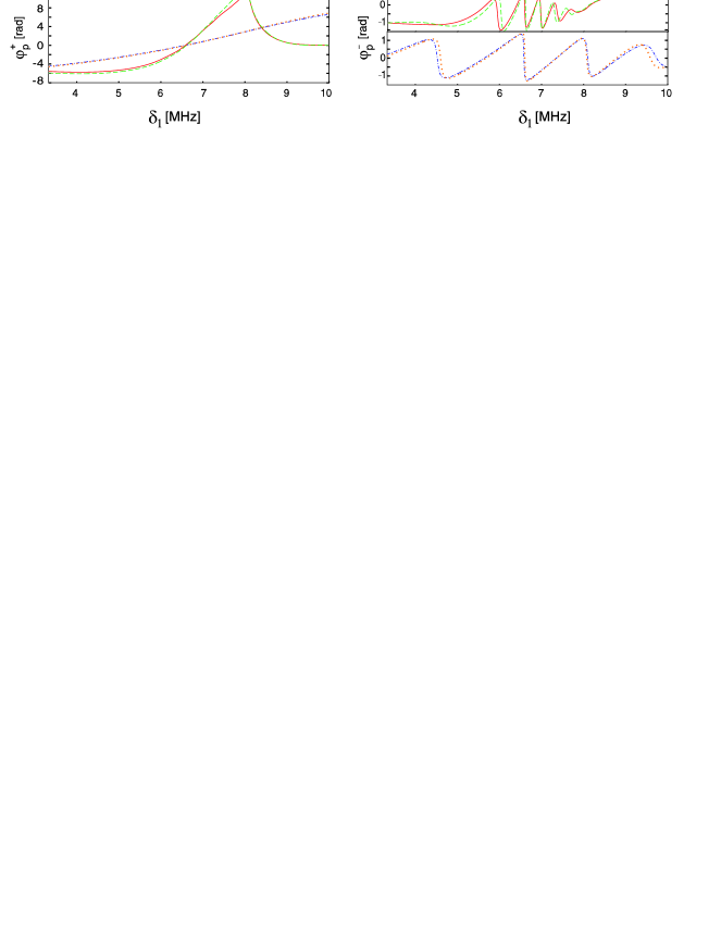
Figure 5: (color online). A comparison of the trigger-induced probe field’s phase shifts (a) $\varphi_{p}^{+}(\delta_{1})$, (b) $\varphi_{p}^{-}(\delta_{1})$, vs the probe detuning $\delta_{1}$ for different control fields: $\Omega_{c}^{+}=6.67$ MHz, trigger present - solid red line, trigger absent - dashed green line, $\Omega_{c}^{+}=10$ MHz, trigger present - dot-dashed blue line, trigger absent - dotted orange line (cf. Fig. 3b, lower plot, in which $\Omega_{c}^{+}=4$ MHz).

We now check how the phase shifts of both the transmitted field and reflected one depend on ’how much standing’ the control field is. We change the right-propagating part of the control field $\Omega_{c}^{+}$ while keeping the left-moving part constant: $\Omega_{c}^{-}=2$ MHz. All the other parameters remain unchanged. The results are shown in Fig. 5a for the transmitted beam and Fig. 5b for the reflected one. All the plots cross in the resonance region where the phase shift is small. The phase shift $\varphi_{p}^{+}$ reaches a maximal value for some $\delta_{1}$ which depends on $\Omega_{c}^{+}$. The more intense is the control field the flatter is the plot and the larger is the peak’s shift towards higher frequencies, which provides a way of controlling the phases. We find the same effect of the peak moving to the right when decreasing the left-propagating part of the control field $\Omega_{c}^{-}$ while keeping $\Omega_{c}^{+}$ constant (not shown). The more intense is the control field the smaller is the trigger-induced phase shift. Around the resonance the reflected phase shift $\varphi_{p}^{-}$ shows an oscillatory dependence on the probe detuning. The width of the frequency range where the oscillations are present grows with $\Omega_{c}^{+}$ but the number of peaks remains constant - again the phase shift’s plot becomes flatter when the control field is increased. The curves are complicated now but roughly we can say that the trigger-induced phase shift decreases when the control field becomes stronger. The extrema of the Kerr phase shifts $\Delta\varphi^{-}_{p}$ in the intervals in which $\varphi_{p}^{-}$ vary rapidly become less prominent and the distance between them increases for growing control fields. In general a too strong control field is not advantegous for generating considerable trigger-induced phase shifts. Then the results gradually turn into those typical of the usual EIT case.

As expected, the transmission coefficient (see Fig. 6a) grows with $\Omega_{c}^{+}$ and so does the width of the transparency window. Again the plots corresponding to the reflection are more complex, as shown in Fig. 6b. In general the reflection coefficient decreases when $\Omega_{c}^{+}$ is increased, but there are some frequency ranges where the dependence is more complicated. Yet if both parts of the control field are increased simultaneously, so that $\frac{\Omega_{c}^{-}}{\Omega_{c}^{+}}$ is constant, then not only the transmission but also the reflection coefficient increases for most of the probe frequencies. This is due to the absorption cancellation by a strong control field.

We have also checked how our results depend on the relaxation rates $\gamma_{ij}$, $j\neq i=1,2,3$, due to interatomic collisions. The main observation is that the trigger-induced phase shift decreases for growing $\gamma_{ij}$. On the other hand, as the relaxation rates grow, the frequency range where the reflected field’s phase dependence is oscillatory becomes wider and the number of oscillations increases. As expected, the transmission and reflection coefficients decrease in general when the relaxation rates grow, but there are some frequency ranges where the reflection coefficient is a nonmonotonic function of $\gamma_{ij}$. Populations $\sigma_{00}$ and $\sigma_{22}$ are negligible except for very large values of the relaxations ($\gamma_{ij}\sim 10^{-1}$ MHz) when they are of the order of a few percent. For increasing $\gamma_{ij}$ the phase shifts become less steep and an approximation consisting in adopting constant values of the populations $\sigma_{11}$ and $\sigma_{33}$ may be better justified.

Increasing the length of the sample leads to increasing the trigger-induced phase shift of the transmitted field. For the considered lengths of the sample the nonlinear phase shift increases for growing $L$. However, for an extended sample both pulses become partially absorbed and their mutual impact is smaller. Elongating the sample leads to no significant change in the amplitude of oscillations in the reflected field’s phase but it does influence the reflection coefficient in a nonmonotonic way, which provides another way of controlling the cross-Kerr effect. Thus, in order to have a considerable phase shift the coupling field cannot be too strong and the relaxation rates between the lower tripod states should not be too large; also the length of the sample should be appropriately optimized.

IV Conclusions

We have presented a comprehensive study of the cross Kerr effect in the propagation of two weak laser fields, a trigger and a probe, in a medium of four-level atoms in the tripod configuration, dressed by a third strong coupling field in the quasi-standing wave configuration. This has been done by taking into the proper account the population redistribution. Using the relevant terms of the Fourier expansion of the linear and nonlinear susceptibilities, we have numerically solved the propagation equations for the right- (incoming) and left- (reflected) running components of the two weak fields. In particular, the phase shifts of the transmitted and reflected probe induced by the trigger turn out to be as large as one radian. We have further shown that the population redistribution significantly affects the phase shifts of the transmitted and reflected beams unless very specific values of probe detuning are used. Over a wide range of probe detunings, on the contrary, we find that the trigger induced phase shifts for the reflected and transmitted probe can be flexibly and independently changed. We have finally characterized the Kerr effect’s dependence on the strength of the coupling field, the relaxation rates and the sample’s length.

In summary, by using a quasi-standing wave configuration the amplitudes of the transmitted and reflected parts of the probe beam and their respective trigger-induced phase shifts can be controlled and optimized by acting on various parameters, and especially on the probe detuning. While previous work has shown the usefulness of the tripod configuration in a running wave EIT regime to achieve a large cross-Kerr effect on the transmitted probe beam, our results extend such findings to the standing wave EIT regime in which both the reflected and transmitted probe beams can be separately controlled.

APPENDIX A

The medium susceptibilities can be written as:

$$\chi_{p} = -\lim_{t\rightarrow\infty}\frac{N|d_{10}|^{2}}{\hbar\epsilon_{0}}\frac{\sigma_{01}}{\Omega_{p}},$$

$$\chi_{t} = -\lim_{t\rightarrow\infty}\frac{N|d_{30}|^{2}}{\hbar\epsilon_{0}}\frac{\sigma_{03}}{\Omega_{t}}.$$

and can be calculated with the use of the steady state solutions of the Bloch equations.

From the last three of Eqs. (1) we find the steady state spin coherences:

$$\sigma_{12}=\frac{\Omega_{c}\sigma_{10}-\Omega_{p}^{*}\sigma_{02}}{\Delta_{12}^{*}},$$

$$\sigma_{32}=\frac{\Omega_{c}\sigma_{30}-\Omega_{t}^{*}\sigma_{02}}{\Delta_{32}^{*}},$$

$$\sigma_{13}=\frac{\Omega_{t}\sigma_{10}-\Omega_{p}^{*}\sigma_{03}}{\Delta_{13}^{*}}.$$

We substitute these expressions into the stationary form of the equations $5-7$ in Eqs. (1) and thus obtain a set of three coupled equations for $\sigma_{10}$, $\sigma_{20}$, $\sigma_{30}$. As the control field is much stronger than any other field present in the system, it prevents the states $0$ and $2$ from being populated. Therefore we set $\sigma_{00}=\sigma_{22}=0$, as was done in Ref. rebic . However, contrary to Ref. rebic , here we do not assume the probe and trigger detunings to be almost equal. Hence the population distribution between the states $1$ and $3$ may be asymmetric and in general $\sigma_{11}\neq\sigma_{33}$. This crucial issue has been discussed in Section III. Next we eliminate $\sigma_{20}$ and arrive at:

$$\left(\Delta_{10}-\frac{|\Omega_{c}|^{2}}{\Delta_{12}}-\frac{|\Omega_{t}|^{2}}{\Delta_{13}}+\frac{|\Omega_{c}|^{2}|\Omega_{p}|^{2}}{D\Delta_{12}^{2}}\right)\sigma_{01}+$$

$$+\frac{\Omega_{t}\Omega_{p}}{\Delta_{13}}\sigma_{30}+\frac{|\Omega_{c}|^{2}\Omega_{p}\Omega_{t}^{*}}{D\Delta_{12}\Delta_{32}}\sigma_{03}=\Omega_{p}\sigma_{11}$$

$$\left(\Delta_{30}-\frac{|\Omega_{c}|^{2}}{\Delta_{32}}-\frac{|\Omega_{p}|^{2}}{\Delta_{31}}+\frac{|\Omega_{c}|^{2}|\Omega_{t}|^{2}}{D\Delta_{32}^{2}}\right)\sigma_{03}+$$

$$+\frac{\Omega_{t}\Omega_{p}}{\Delta_{31}}\sigma_{10}+\frac{|\Omega_{c}|^{2}\Omega_{t}\Omega_{p}^{*}}{D\Delta_{12}\Delta_{32}}\sigma_{01}=\Omega_{t}\sigma_{33}$$

where $D=\Delta_{20}^{*}+\frac{|\Omega_{p}|^{2}}{\Delta_{12}}+\frac{|\Omega_{t}|^{2}}{\Delta_{32}}$.

We combine the above expressions to obtain $\frac{\sigma_{01}}{\Omega_{p}}$ and $\frac{\sigma_{03}}{\Omega_{t}}$. The solutions of the above set of equations expanded into the Taylor series have the form of Eq. (4), with:

$$\chi_{p}^{(1)}(\delta_{1}) = -\frac{N|d_{10}|^{2}\sigma_{11}}{\hbar\epsilon_{0}}\frac{\Delta_{12}}{\Delta_{10}\Delta_{12}-|\Omega_{c}|^{2}},$$ (A.1)

$$\chi_{pp}^{(3)}(\delta_{1}) = \frac{N|d_{10}|^{2}}{\hbar\epsilon_{0}}\frac{\sigma_{11}}{\Delta_{20}^{*}}\frac{|\Omega_{c}|^{2}}{(\Delta_{10}\Delta_{12}-|\Omega_{c}|^{2})^{2}},$$ (A.2)

$$\chi_{pt}^{(3)}(\delta_{1}) = -\frac{N|d_{10}|^{2}}{\hbar\epsilon_{0}}\left[\frac{\Delta_{12}}{\Delta_{13}}\frac{1}{\Delta_{10}\Delta_{12}-|\Omega_{c}|^{2}}\right.\times$$

$$\times \left(\frac{\sigma_{11}\Delta_{12}}{\Delta_{10}\Delta_{12}-|\Omega_{c}|^{2}}+\frac{\sigma_{33}\Delta_{23}}{-\Delta_{30}^{*}\Delta_{23}-|\Omega_{c}|^{2}}\right)-$$

$$- \left.\frac{\sigma_{33}}{\Delta_{20}^{*}}\frac{|\Omega_{c}|^{2}}{(\Delta_{10}\Delta_{12}-|\Omega_{c}|^{2})(\Delta_{30}\Delta_{32}-|\Omega_{c}|^{2})}\right].$$

The trigger susceptibilities are obtained by interchanging the indices $\{p,1\}\leftrightarrow\{t,3\}$.

For the control field being in the form of a quasi-standing wave $\Omega_{c}=\Omega_{c}^{+}e^{ik_{2}z}+\Omega_{c}^{-}e^{-ik_{2}z}$ the medium susceptibilities can be then expanded into the Fourier series:

$$\chi_{p}^{(1)}=\chi_{p,0}^{(1)}+2\sum_{n=1}^{\infty}\chi_{p,2n}^{(1)}\cos(2nk_{c}z),$$

and similarly for $\chi_{pt,2n}^{(3)}$, etc. To find the explicit form of the Fourier coefficients we rewrite the expressions (A.1 - IV):

$$\chi_{p}^{(1)} = \frac{N|d_{10}|^{2}\sigma_{11}}{\hbar\epsilon_{0}}\frac{A\Delta_{12}}{1+B\cos(2k_{c}z)},$$

$$\chi_{pt}^{(3)} = -\frac{N|d_{10}|^{2}}{\hbar\epsilon_{0}}\left[\frac{\nu}{(1+B\cos(2k_{c}z))^{2}}\right.-$$

$$- \frac{\eta A}{1+B\cos(2k_{c}z)}+\frac{\eta C}{1+D\cos(2k_{c}z)}+$$

$$+ \left(\frac{\eta^{\prime}A}{1+B\cos(2k_{c}z)}-\frac{\eta^{\prime}C^{*}}{1+D^{*}\cos(2k_{c}z)}\right)\times$$

$$\times \left.\left(S_{c}^{2}+2\Omega_{c}^{+}\Omega_{c}^{-}\cos(2k_{c}z)\right)\right],$$

$$\chi_{pp}^{(3)} = \frac{N|d_{10}|^{2}}{\hbar\epsilon_{0}}\frac{\nu^{\prime}}{\Delta_{20}^{*}}\frac{S_{c}^{2}+2\Omega_{c}^{+}\Omega_{c}^{-}\cos 2k_{c}z}{\left[1+B\cos(2k_{c}z)\right]^{2}},$$

where: $A=\left(S_{c}^{2}-\Delta_{10}\Delta_{12}\right)^{-1}$, $B=2\Omega_{c}^{+}\Omega_{c}^{-}A$, $S_{c}^{2}={\Omega_{c}^{+}}^{2}+{\Omega_{c}^{-}}^{2}$, $\nu=\frac{\Delta_{12}^{2}}{\Delta_{13}}\nu^{\prime}$, $\nu^{\prime}=\sigma_{11}A^{2}$, $\eta=-\frac{\sigma_{33}\Delta_{12}\Delta_{23}/\Delta_{13}}{\Delta_{30}^{*}\Delta_{23}+\Delta_{10}\Delta_{12}}$, $\eta^{\prime}=\frac{\sigma_{33}/\Delta_{20}^{*}}{\Delta_{30}\Delta_{32}-\Delta_{10}\Delta_{12}}$, $C=\left(S_{c}^{2}+\Delta_{30}^{*}\Delta_{23}\right)^{-1},D=2\Omega_{c}^{+}\Omega_{c}^{-}C$.

Let us denote:

$$F^{(1)}_{n}(\mu) \equiv \frac{1}{2\pi}_{-\pi}\int^{\pi}\frac{\cos(nx)dx}{1+\mu\cos(x)}=\frac{1}{\sqrt{1-\mu^{2}}}\left(\frac{\sqrt{1-\mu^{2}}-1}{\mu}\right)^{n},$$

$$F^{(2)}_{0}(\mu) \equiv \frac{1}{2\pi}_{-\pi}\int^{\pi}\frac{dx}{[1+\mu\cos(x)]^{2}}=\frac{1}{\sqrt{1-\mu^{2}}^{3}},$$

$$F^{(2)}_{1}(\mu) \equiv \frac{1}{2\pi}_{-\pi}\int^{\pi}\frac{\cos(x)dx}{[1+\mu\cos(x)]^{2}}=\frac{-\mu}{\sqrt{1-\mu^{2}}^{3}},$$

$$F^{(2)}_{2}(\mu) \equiv \frac{1}{2\pi}_{-\pi}\int^{\pi}\frac{\cos(2x)dx}{[1+\mu\cos(x)]^{2}}=\frac{2}{\mu^{2}}+\frac{3-\frac{2}{\mu^{2}}}{\sqrt{1-\mu^{2}}^{3}},$$

$$F^{(2)}_{3}(\mu) \equiv \frac{1}{2\pi}_{-\pi}\int^{\pi}\frac{\cos(3x)dx}{[1+\mu\cos(x)]^{2}}=-\frac{8}{\mu^{3}}+\frac{\frac{8}{\mu^{3}}-\frac{12}{\mu}+3\mu}{\sqrt{1-\mu^{2}}^{3}}.$$

The above integrals have been calculated with the use of the residues method. The Fourier coefficients of the susceptibilities read then:

$$\chi_{p,2n}^{(1)} = \frac{N\sigma_{11}|d_{10}|^{2}}{\hbar\epsilon_{0}}A\Delta_{12}F^{(1)}_{n}(B),$$

$$\chi_{pt,0}^{(3)} = -\frac{N|d_{10}|^{2}}{\hbar\epsilon_{0}}\left[\nu F^{(2)}_{0}(B)\right.-$$

$$- \eta\left(AF^{(1)}_{0}(B)-CF^{(1)}_{0}(D)\right)$$

$$+ \eta^{\prime}S_{c}^{2}\left(AF^{(1)}_{0}(B)-C^{*}F^{(1)}_{0}(D^{*})\right)+$$

$$+ \left.\eta^{\prime}2\Omega_{c}^{+}\Omega_{c}^{-}\left(AF^{(1)}_{1}(B)-C^{*}F^{(1)}_{1}(D^{*})\right)\right],$$

$$\chi_{pt,2}^{(3)} = -\frac{N|d_{10}|^{2}}{\hbar\epsilon_{0}}\left[\nu F^{(2)}_{1}(B)\right.-$$

$$- \eta\left(AF^{(1)}_{1}(B)-CF^{(1)}_{1}(D)\right)$$

$$+ \eta^{\prime}S_{c}^{2}\left(AF^{(1)}_{1}(B)-C^{*}F^{(1)}_{1}(D^{*})\right)+$$

$$+ \eta^{\prime}\Omega_{c}^{+}\Omega_{c}^{-}A\left(F^{(1)}_{0}(B)+F^{(1)}_{2}(B)\right)-$$

$$- \left.\eta^{\prime}\Omega_{c}^{+}\Omega_{c}^{-}C^{*}\left(F^{(1)}_{0}(D^{*})+F^{(1)}_{2}(D^{*})\right)\right],$$

$$\chi_{pt,4}^{(3)} = -\frac{N|d_{10}|^{2}}{\hbar\epsilon_{0}}\left[\nu F^{(2)}_{2}(B)\right.-$$

$$- \eta\left(AF^{(1)}_{2}(B)-CF^{(1)}_{2}(D)\right)+$$

$$+ \eta^{\prime}S_{c}^{2}\left(AF^{(1)}_{2}(B)-C^{*}F^{(1)}_{2}(D^{*})\right)-$$

$$+ \eta^{\prime}\Omega_{c}^{+}\Omega_{c}^{-}A\left(F^{(1)}_{1}(B)+F^{(1)}_{3}(B)\right)-$$

$$- \left.\eta^{\prime}\Omega_{c}^{+}\Omega_{c}^{-}C^{*}\left(F^{(1)}_{1}(D^{*})+F^{(1)}_{3}(D^{*})\right)\right],$$

$$\chi_{pp,0}^{(3)} = \frac{N|d_{10}|^{2}}{\hbar\epsilon_{0}}\frac{\nu^{\prime}}{\Delta_{20}^{*}}\left[S_{c}^{2}F^{(2)}_{0}(B)+2\Omega_{c}^{+}\Omega_{c}^{-}F^{(2)}_{1}(B)\right],$$

$$\chi_{pp,2}^{(3)} = \frac{N|d_{10}|^{2}}{\hbar\epsilon_{0}}\frac{\nu^{\prime}}{\Delta_{20}^{*}}\left[S_{c}^{2}F^{(2)}_{1}(B)+\Omega_{c}^{+}\Omega_{c}^{-}\left(F^{(2)}_{0}(B)+F^{(2)}_{2}(B)\right)\right],$$

$$\chi_{pp,4}^{(3)} = \frac{N|d_{10}|^{2}}{\hbar\epsilon_{0}}\frac{\nu^{\prime}}{\Delta_{20}^{*}}\left[S_{c}^{2}F^{(2)}_{2}(B)+\Omega_{c}^{+}\Omega_{c}^{-}\left(F^{(2)}_{1}(B)+F^{(2)}_{3}(B)\right)\right],$$

As shown above, only these coefficients are present in the pulse propagation equations. Note that the corresponding formulae given in Ref. myScripta included some misprints.

APPENDIX B

To evaluate the population redistribution we proceed as follows. We first use equations 2-4 of the stationary version of Eqs. (1) to express $\sigma_{00}$ through $\sigma_{j0}$ and $\sigma_{jj}$:

$$\sigma_{00} = \frac{2}{\gamma_{11}}\Im(\Omega_{p}\sigma_{10})+\xi(\sigma_{11}-\sigma_{33}),$$

$$= \frac{2}{\gamma_{22}}\Im(\Omega_{c}\sigma_{20})-\xi(\sigma_{11}+\sigma_{33}),$$

$$= \frac{2}{\gamma_{33}}\Im(\Omega_{t}\sigma_{30})+2\xi\sigma_{33},$$

where $\xi=\frac{\gamma_{ij}}{\gamma_{kk}}$, $i,j,k=1,2,3$. Note that here we do not assume any of the populations negligible. Next we express $\sigma_{j0}$ through the diagonal elements of $\sigma$ in the lowest-order approximation with respect to the probe and trigger:

$$\sigma_{10} = \frac{\Omega_{p}^{*}(\sigma_{11}-\sigma_{00})}{\Delta_{10}^{*}-\frac{|\Omega_{c}|^{2}}{\Delta_{12}^{*}}}-\frac{\Omega_{p}^{*}|\Omega_{c}|^{2}(\sigma_{22}-\sigma_{00})}{D^{*}(\Delta_{10}^{*}\Delta_{12}^{*}-|\Omega_{c}|^{2})},$$

$$\sigma_{20} = \frac{\Omega_{c}^{*}}{D}\left[(\sigma_{22}-\sigma_{00})+\frac{|\Omega_{p}|^{2}(\sigma_{11}-\sigma_{00})}{\Delta_{10}\Delta_{12}-|\Omega_{c}|^{2}}-\frac{|\Omega_{p}|^{2}|\Omega_{c}|^{2}(\sigma_{22}-\sigma_{00})}{\Delta_{12}D(\Delta_{10}\Delta_{12}-|\Omega_{c}|^{2})}+\right.$$

$$+ \left.\frac{|\Omega_{t}|^{2}(\sigma_{33}-\sigma_{00})}{\Delta_{30}\Delta_{32}-|\Omega_{c}|^{2}}-\frac{|\Omega_{t}|^{2}|\Omega_{c}|^{2}(\sigma_{22}-\sigma_{00})}{\Delta_{32}D(\Delta_{30}\Delta_{32}-|\Omega_{c}|^{2})}\right],$$

$$\sigma_{30} = \frac{\Omega_{t}^{*}(\sigma_{33}-\sigma_{00})}{\Delta_{30}^{*}-\frac{|\Omega_{c}|^{2}}{\Delta_{32}^{*}}}-\frac{\Omega_{t}^{*}|\Omega_{c}|^{2}(\sigma_{22}-\sigma_{00})}{D^{*}(\Delta_{30}^{*}\Delta_{32}^{*}-|\Omega_{c}|^{2})},$$

where $D=\Delta_{20}^{*}+\frac{|\Omega_{p}|^{2}}{\Delta_{12}}+\frac{|\Omega_{t}|^{2}}{\Delta_{32}}$. Combining the two latter steps we obtain a set of linear equations for the diagonal elements:

$$\sigma_{00} = \alpha(\sigma_{11}-\sigma_{00})-\alpha_{1}(\sigma_{22}-\sigma_{00})+\xi(\sigma_{11}-\sigma_{33}),$$

$$\sigma_{00} = \beta(\sigma_{33}-\sigma_{00})-\beta_{1}(\sigma_{22}-\sigma_{00})+2\xi\sigma_{33},$$ (B.1)

$$\sigma_{00} = \gamma(\sigma_{11}-\sigma_{00})+\delta(\sigma_{33}-\sigma_{00})+\epsilon(\sigma_{22}-\sigma_{00}),$$

$$\sigma_{00} + \sigma_{11}+\sigma_{22}+\sigma_{33}=1,$$

where:

$$\alpha = \frac{2}{\gamma_{11}}|\Omega_{p}|^{2}\Im\left(\frac{1}{\Delta_{10}^{*}-\frac{|\Omega_{c}|^{2}}{\Delta_{12}^{*}}}\right),$$

$$\alpha_{1} = \frac{2}{\gamma_{11}}|\Omega_{p}|^{2}|\Omega_{c}|^{2}\Im\left(\frac{1}{D^{*}(\Delta_{10}^{*}\Delta_{12}^{*}-|\Omega_{c}|^{2})}\right),$$

$$\beta = \frac{2}{\gamma_{33}}|\Omega_{t}|^{2}\Im\left(\frac{1}{\Delta_{30}^{*}-\frac{|\Omega_{c}|^{2}}{\Delta_{32}^{*}}}\right),$$

$$\beta_{1} = \frac{2}{\gamma_{33}}|\Omega_{t}|^{2}|\Omega_{c}|^{2}\Im\left(\frac{1}{D^{*}(\Delta_{30}^{*}\Delta_{32}^{*}-|\Omega_{c}|^{2})}\right),$$

$$\gamma = \frac{2}{\gamma_{22}}|\Omega_{c}|^{2}|\Omega_{p}|^{2}\Im\left(\frac{1}{D(\Delta_{10}\Delta_{12}-|\Omega_{c}|^{2})}\right),$$ (B.2)

$$\delta = \frac{2}{\gamma_{22}}|\Omega_{c}|^{2}|\Omega_{t}|^{2}\Im\left(\frac{1}{D(\Delta_{30}\Delta_{32}-|\Omega_{c}|^{2})}\right),$$

$$\epsilon = \frac{2}{\gamma_{22}}|\Omega_{c}|^{2}\left[\Im\left(\frac{1}{D}\right)-|\Omega_{c}|^{2}|\Omega_{p}|^{2}\Im\left(\frac{1}{\Delta_{12}D^{2}(\Delta_{10}\Delta_{12}-|\Omega_{c}|^{2})}\right)-\right.$$

$$+ \left.|\Omega_{c}|^{2}|\Omega_{t}|^{2}\Im\left(\frac{1}{\Delta_{32}D^{2}(\Delta_{30}\Delta_{32}-|\Omega_{c}|^{2})}\right)\right].$$

The solutions of Eqs. (B.1) are

$$\sigma_{11} = \frac{1}{M}\left\{(1+\alpha)(\beta_{1}\delta+\beta\epsilon)+(3+2\alpha+\beta)\epsilon\xi+\beta_{1}(-\alpha+\delta+\gamma)\xi+\right.$$

$$+ \left.\alpha_{1}\left[-\delta+3\xi+2(\delta+\gamma)\xi+\beta(1+\gamma+\xi)\right]\right\},$$

$$\sigma_{22} = \frac{1}{M}\left\{(-1+\alpha_{1})\beta\gamma+\left[(-1+\beta_{1})\delta+\beta(2-\alpha_{1}+\epsilon)+\gamma(-3+2\alpha_{1}+\beta_{1})\right]\xi+\right.$$ (B.3)

$$+ 2(3-\alpha_{1}-\beta_{1}+\beta+\delta+\gamma+\epsilon)\xi^{2}+$$

$$+ \left.\alpha\left[(-1+\beta_{1})\delta+(3-\beta_{1})\xi+2\xi(\delta+\epsilon+\xi)+\beta(1+\epsilon+2\xi)\right]\right\},$$

$$\sigma_{33} = \frac{1}{M}\left\{-\beta_{1}\gamma+\alpha_{1}(1+\beta)(\gamma-\xi)+\left[(1+\beta)\epsilon+\beta_{1}(2+\delta+\gamma)\right]\xi+\right.$$

$$+ \left.\alpha\left[(1+\beta)\epsilon+\beta_{1}(1+\delta+\epsilon)\right]\right\},$$

while the value of $\sigma_{00}$ follows from the probability conservation. The denominator $M$ reads:

$$M = \beta_{1}(\delta-\gamma)+\beta(\epsilon-\gamma+4\alpha_{1}\gamma)+\alpha_{1}(\beta+\gamma-\delta)+$$

$$+ \left[2\beta-\delta+4\epsilon+4\beta\epsilon-3\gamma+2\alpha_{1}(1-\beta+3\gamma+\delta)+\beta_{1}(2+4\gamma+4\delta)\right]\xi+$$

$$+ 2(3-2\alpha_{1}-2\beta_{1}+\beta+\gamma+\delta+2\epsilon)\xi^{2}+$$

$$+ \alpha\left[\beta-\delta+\epsilon+4\beta\epsilon+\beta_{1}(1+4\delta-2\xi)+3\xi+2\xi(\beta+\delta+3\epsilon+\xi)\right].$$

Using the above equations with constant initial values of probe and trigger fields and a given value of the control field we are able to estimate the population distribution.

References

Figure 6: (color online). Transmission (a) and reflection (b) coefficients in the presence of a trigger and for different values of the control field $\Omega_{c}^{+}=4$ MHz (solid red), $\Omega_{c}^{+}=5.33$ MHz (dashed green), $\Omega_{c}^{+}=6.67$ MHz (dotted blue) when the other coupling beam is set to $\Omega_{c}^{-}=2$ MHz.