Abstract

Multiplication of spin qubits arises at double resonance in a bichromatic field when the frequency of the radio-frequency (rf) field is close to that of the Rabi oscillation in the microwave field, provided its frequency equals the Larmor frequency of the initial qubit. We show that the operational multiphoton transitions of dressed qubits can be selected by the choice of both the rotating frame and the rf phase. In order to enhance the precision of dressed qubit operations in the strong-field regime, the counter-rotating component of the rf field is taken into account.

PACS: 03.67.Pp, 33.40.+f, 33.35.+r

Theoretical models of quantum computations assume the existence of an ideal two-level quantum system (qubit) and the possibility of an exact description of the qubit’s interaction with external electromagnetic fields [1]. It is known that the resonant interaction between electromagnetic radiation and qubit induces Rabi oscillations, which are the basis for quantum operations. The Rabi frequency $\omega_{R}$ is defined by the amplitude of the electromagnetic field and usually is much smaller than the energy difference $\omega_{0}$ (in frequency units) between the qubit’s states. The ”dressing” of qubit by the electromagnetic field splits each level into two giving rise to two new qubits with energy difference $\omega_{R}$. The spectrum of the multilevel ”qubit + field” system consists of three lines at the frequencies $\omega_{0}$ and $\omega_{0}\pm\omega_{R}$ (the Mollow triplet [2]). The second low-frequency electromagnetic field with the frequency close to the Rabi frequency $\omega_{R}$ could induce an additional Rabi oscillation on dressed states of new qubits. These qubits are attracting interest because their coherence time is longer than that of the initial qubit  [3 – 5]. The results of studies of qubits dressed by bichromatic radiation formed by fields with strongly different frequencies are important for a wide range of physical objects, including, among others, nuclear and electron spins, double-well quantum dots, flux and charge qubits in superconducting systems. In NMR [6, 7], EPR [5, 8, 9] and optical resonance [10] such investigations are used in the development of line-narrowing methods.

In this letter, we describe the multiplication of spin qubits at double resonance in a bichromatic field with strongly different frequencies. We then show that the operational multiphoton transitions of dressed qubits can be selected by the choice of both the rotating frame and the phase of the low-frequency field. Two important examples of such transitions in the rotating and doubly rotating frames are presented.

Let an electron spin qubit be in three fields: a microwave (mw) one directed along the x axis of the laboratory frame, a radio-frequency (rf) one directed along the $z$ axis, and a static magnetic one also directed along the $z$ axis. The Hamiltonian of the qubit in these fields can be written as follows:

$$H=H_{0}+H_{\bot}\left(t\right)+H_{\parallel}\left(t\right).$$ (1)

Here $H_{0}=\omega_{0}s^{z}$ is the Hamiltonian of the Zeeman energy of a spin in the static magnetic field $B_{0}$, where $\omega_{0}=\gamma B_{0}$, and $\gamma$ is the electron gyromagnetic ratio. Moreover, $H_{\bot}\left(t\right)=2\omega_{1}\cos\left(\omega t+\phi\right)s^{x}$ and $H_{\parallel}\left(t\right)=2\omega_{2}\cos\left(\omega_{rf}t+\psi\right)s^{z}$ are the Hamiltonians of the spin interaction with linearly polarized mw and rf fields, respectively. $B_{1}$ and $B_{2}$, $\omega$ and $\omega_{rf}$, and $\varphi$ and $\psi$ denote the respective amplitudes, frequencies, and phases of the mw and rf fields. Finally, $\omega_{1}=\gamma B_{1}$ and $\omega_{2}=\gamma B_{2}$ stand for the Rabi frequencies, whereas $s^{x,y,\,z}$ are the components of the spin operator.

The evolution of the system with the Hamiltonian 1 is described by the Liouville equation for the density matrix $\rho$:

$$i\frac{\partial\rho}{\partial t}=[H,\rho]$$ (2)

(we set the Planck constant $\hbar=1$). We perform the transformation ($\rho\to\rho_{1}=U_{1}^{+}\rho U_{1}$, $U_{1}=e^{-i\omega ts^{z}}$) to the singly rotating frame, which rotates with frequency $\omega$ around the z axis of the laboratory frame. In this frame, Eq. 2 turns into:

$$i\frac{\partial\rho_{1}}{\partial t}=[H_{1},\rho_{1}],$$ (3)

where $H_{1}=U_{1}^{+}HU_{1}=\Delta s^{z}+(\omega_{1}/2)(s^{+}+s^{-})+2\omega_{2}\cos(\omega_{rf}t+\psi)s^{z}$ and $\Delta=\omega_{0}-\omega$. The mw phase $\varphi=0$ and the counter-rotating component of the mw field is neglected. We also assume that the exact resonance condition is fulfilled $\Delta=0$, and that $\omega_{1}$, $\omega_{rf}\gg\omega_{2}$. Upon rotation of the frame around the y axis by the angle of $\pi/2$ ($\rho_{1}\to\rho_{2}=U_{2}^{+}\rho_{1}U_{2}$, $U_{2}=e^{-i\pi s^{y}/2}$, where $s^{y}=(s^{+}-s^{-})/2i$), we obtain:

$$i\frac{\partial\rho_{2}}{\partial t}=[H_{2},\rho_{2}],$$ (4)

where $H_{2}=U_{2}^{+}H_{1}U_{2}=\omega_{1}s^{z}-\omega_{2}\cos(\omega_{rf}t+\psi)(s^{+}+s^{-})$.

Now, we pass to the interaction representation by choosing the frame rotating with frequency $\omega_{1}$ around the $z$ axis ($\rho_{2}\to\rho_{3}=U_{3}^{+}\rho_{2}U_{3}$, $U_{3}=e^{-i\omega_{1}ts^{z}}$). In this frame we have:

$$i\frac{\partial\rho_{3}}{\partial t}=[H_{3},\rho_{3}],$$ (5)

where

$H_{3}=U_{3}^{+}H_{2}U_{3}=-(\omega_{2}/2)s^{+}\left(e^{i\delta t}e^{-i\psi}+e^{i(2\omega_{rf}+\delta)t}e^{i\psi}\right)-h.c.$, $\delta=\omega_{1}-\omega_{rf}$, and $\left|\delta\right|\ll\omega_{1},\,\omega_{rf}$ in our case. Rapidly oscillating ($e^{\pm i2\omega_{rf}t}$) terms in the Hamiltonian $H_{3}$ can be eliminated by the Krylov–Bogoliubov–Mitropolsky method [5, 11, 12]. Averaging over the period $2\pi/\omega_{rf}$, we obtain the following effective Hamiltonian up to the second order in $\omega_{2}/\omega_{rf}$:

$$H_{3}\to H_{eff}=H_{eff}^{(1)}+H_{eff}^{(2)}.$$ (6)

In the above equation we have put:

$H_{eff}^{\ref{GrindEQ__1_}}=\langle H_{3}(t)\rangle=-(\omega_{2}/2)(s^{+}e^{i\delta t}e^{-i\psi}+h.c.)$, $H_{eff}^{\ref{GrindEQ__2_}}=\frac{i}{2}\langle[\int^{t}d\tau\left(H_{3}(\tau)-\langle H_{3}(\tau)\rangle\right),\,H_{3}(t)]\rangle=\Delta_{BS}s^{z}$. The symbol $<...>$ denotes time averaging: $\langle A(t)\rangle={\frac{1}{T}}\int_{0}^{T}A(t)dt$, where $T=2\pi/\omega_{rf}$ and $\Delta_{BS}\approx\omega_{2}^{2}/4\omega_{rf}$ is the Bloch–Siegert-like frequency shift.

After the canonical transformation $\rho_{3}\to\rho_{4}=U_{4}^{+}\rho_{3}U_{4}$, $U_{4}=e^{-i(\delta t-\psi)s^{z}}$, the equation

$$i\frac{\partial\rho_{3}}{\partial t}=[H_{eff},\rho_{3}]$$ (7)

is transformed into

$$i\frac{\partial\rho_{4}}{\partial t}=[H_{4},\rho_{4}],$$ (8)

where $H_{4}=U_{4}^{+}H_{eff}U_{4}=(\delta+\Delta_{BS})s^{z}-(\omega_{2}/2)(s^{+}+s^{-})$.

The diagonalization of the Hamiltonian $H_{4}$ by means of the rotation operator $U_{5}=e^{-i\xi s^{y}}$ ($\rho_{5}\to\rho_{5}=U_{5}^{+}\rho_{4}U_{5}$, $H_{5}=U_{5}^{+}H_{4}U_{5}$) yields:

$$i\frac{\partial\rho_{5}}{\partial t}=[H_{5},\rho_{5}].$$ (9)

Here $H_{5}=\varepsilon s^{z}$, $\varepsilon=\sqrt{(\omega_{1}-\omega_{rf}+\Delta_{BS})^{2}+\omega_{2}^{2}}$ is the frequency of the Rabi oscillations between the spin states dressed simultaneously by the mw and rf field while $\sin\xi=-\omega_{2}/\varepsilon$, $\cos\xi=(\omega_{1}-\omega_{rf}+\Delta_{BS})/\varepsilon$.

By using Eqs. 2 – 9, the density matrix in the laboratory frame (LF) can be written as:

$$\rho(t)=U_{1}U_{2}U_{3}U_{4}U_{5}e^{-iH_{5}t}\rho_{5}(0)e^{iH_{5}t}U_{5}^{+}U_{4}^{+}U_{3}^{+}U_{2}^{+}U_{1}^{+},$$ (10)

where

$$\rho_{5}(0)=U_{5}^{+}U_{4}^{+}(0)U_{3}^{+}(0)U_{2}^{+}U_{1}^{+}(0)\rho(0)U_{5}U_{4}(0)U_{3}(0)U_{2}U_{1}(0),$$ (11)

and $U_{1}(0)=1$, $U_{3}(0)=1$, $U_{4}(0)=e^{-i\psi s^{z}}$.

Initially, the qubit is in the ground state and $\rho(0)=1/2-s^{z}$. The absorption signal $\upsilon(t)=Sp\{\rho(t)(s^{+}-s^{-})\}/2i$ in the laboratory frame can be derived from Eqs. 10 and 11:

$$\upsilon(t)=\left(\langle 1|\rho(t)|2\rangle-\langle 2|\rho(t)|1\rangle\right)/2i=$$

$$=(1/2)\sin\xi\cos\xi\cos\psi\sin\omega t+(1/16)\{4\sin\xi\sin\psi[\cos(\omega+\varepsilon)t-\cos(\omega-\varepsilon)t]+$$

$$-4\sin\xi\cos\xi\cos\psi[\sin(\omega-\varepsilon)t+\sin(\omega+\varepsilon)t]+2\sin^{2}\xi\sin 2\psi[\cos(\omega+\omega_{rf})t+\cos(\omega-\omega_{rf})t]+$$

$$+\left(\left(\cos\xi-1\right)^{2}+\left(\cos^{2}\xi-1\right)\cos 2\psi\right)\times[\sin(\omega+\omega_{rf}-\varepsilon)t-\sin(\omega-\omega_{rf}+\varepsilon)t]+$$

$$+\left(\cos^{2}\xi-1\right)\sin 2\psi\times[\cos(\omega-\omega_{rf}+\varepsilon)t+\cos(\omega+\omega_{rf}-\varepsilon)t]+$$

$$+\left(\left(\cos\xi+1\right)^{2}+\left(\cos^{2}\xi-1\right)\cos 2\psi\right)\times[\sin(\omega+\omega_{rf}+\varepsilon)t-\sin(\omega-\omega_{rf}-\varepsilon)t]+$$

$$+\left(\cos^{2}\xi-1\right)\sin 2\psi\times[\cos(\omega-\omega_{rf}-\varepsilon)t+\cos(\omega+\omega_{rf}+\varepsilon)t]\}.$$ (12)

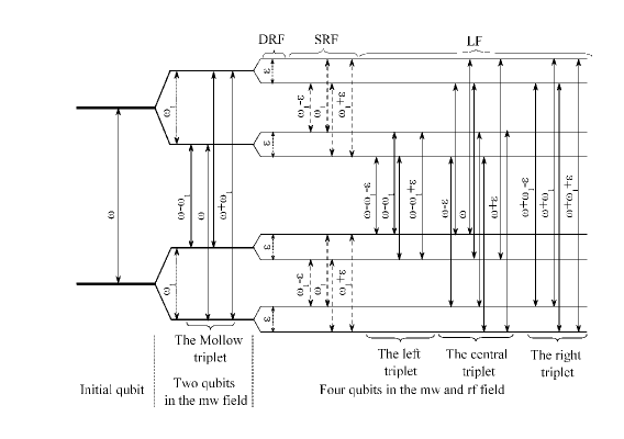
Figure 1: Energy-level diagram of a qubit and transitions created by a bichromatic field at double resonance ($\omega_{0}=\omega$, $\omega_{1}=\omega_{rf}$).

The resonant interaction between the mw field and the qubit creates its dressed states and two new qubits with energy splitting equal to the Rabi frequency $\omega_{1}$, as shown in Fig.1. The rf field with the frequency $\omega_{rf}$, which is close to the Rabi frequency $\omega_{1}$ of the new qubits, ”dresses” these qubits, giving rise to four qubits with the energy splitting $\epsilon$. Allowed transitions between states of these qubits afford nine spectral lines observed in the laboratory frame.

Figs. 2 and 3 show the time evolution of absorption signals and their Fourier spectra of dressed qubits under conditions typical for EPR.

Figure 2: Time evolution of the absorption signals in the laboratory (solid line), singly rotating (dot line) and doubly rotating (dash line) frames. The signals were obtained for the following parameters of the bichromatic field: $\omega=\omega_{0}$, $\omega_{1}=\omega_{rf}=2\pi$1.0 MHz, $\omega_{2}=2\pi$0.24 MHz, using the exponential decay function with T = 16 $\mu$s.	Figure 3: Fourier spectra of the absorption signals in the laboratory frame shown in Fig. 2 by a solid line.

For the rf phase $\psi=0$, three triplets with the intensive central lines at $\omega-\omega_{1}$, $\omega$ and $\omega+\omega_{1}$ are formed (Fig. 3a). The less intensive sidebands have the frequencies $\pm\varepsilon$ relative to each of the central lines. For the rf phase $\psi=\pi/2$, the central lines in the triplets vanish (Fig. 3b), each triplet turning into an doublet. When the rf phase is random, averaging over a sufficiently large number of experiments (at the uniform distribution of the phase in the interval from 0 to 2$\pi$) leads to a complete removal of the central triplet. The differences of line’s intensities in the two residual triplets ($\omega-\omega_{1}$, $\omega-\omega_{1}\pm\varepsilon$ and $\omega+\omega_{1}$, $\omega+\omega_{1}\pm\varepsilon$) become smaller (Fig. 3c).

There is the possibility of selecting the observed transitions of four qubits by employing the rotating frame. In the singly rotating frame (SRF), the absorption signal described by the density matrix $\rho_{1}(t)$ (Eq. (4)) can by written as

$$\begin{array}[]{l}{\upsilon_{1}\left(t\right)=(1/8)\left[2\sin^{2}\xi\left(\sin\omega_{rf}t+\sin\left(\omega_{rf}t+2\psi\right)\right)+\right.}\\ {+\left(1+\cos\xi\right)^{2}\sin\left(\omega_{rf}+\varepsilon\right)t-}\\ {-\left(1-\cos^{2}\xi\right)\sin\left(\left(\omega_{rf}+\varepsilon\right)t+2\psi\right)+}\\ {\left.+\left(1-\cos\xi\right)^{2}\sin\left(\omega_{rf}-\varepsilon\right)t-\right.}\\ {\left.-\left(1-\cos^{2}\xi\right)\sin\left(\left(\omega_{rf}-\varepsilon\right)t+2\psi\right)\right].}\end{array}$$ (13)

Fig. 4 shows the Fourier spectra of signals given by Eq. 13 under the same conditions as in Figs. 2 and 3. For the random rf phase, the absorption signal has three comparable oscillating components with frequencies $\omega_{1}$ and $\omega_{1}\pm\sqrt{\omega_{2}^{2}+\Delta_{BS}^{2}}$ (Fig. 4c). For the rf phase $\psi=0$, the sidebands are smaller than those at the random rf phase by the factor $\Delta_{BS}/\sqrt{\omega_{2}^{2}+\Delta_{BS}^{2}}$ (Fig. 4a). When we use $\psi=\pi/2$, the component with frequency $\omega_{1}$ vanishes and the sidebands are comparable to those at the random rf phase (Fig. 4b). Note that the high-frequency sideband is always more intensive than the low-frequency one.

Figure 4: Fourier spectra of the absorption signals in the singly rotating frame shown in Fig. 2 by a dot line.

Upon the rotating wave approximation ($\Delta_{BS}\to 0$), it follows from Eq. 13 that for $\psi=0$ only the component with frequency $\omega_{1}$ remains. At the same time, for both $\psi=\pi/2$ and the random rf phase, the intensities of the sidebands are equal. The equalization of sidebands can be used to indicate the validity of the rotating wave approximation. On the contrary, their asymmetry reveals the effect of the counter-rotating component of the rf field. Such asymmetry was observed in the dressed Rabi oscillations using the EPR experiment with random rf phase [5].

Note that, upon the resonant monochromatic interaction, the Mollow triplet is formed by the transitions between the dressed states of the ground and excited levels of the initial qubit. Similarly, at the doubly resonant bichromatic interaction, the triplet in the singly rotating frame is formed by the transitions between the split states of both the ground and excited levels of the initial qubit (Fig. 1).

We now provide the expression for the absorption signal in the frame described by the density matrix $\rho_{5}(t)=e^{-iH_{5}t}\rho_{5}(0)e^{iH_{5}t}$, where $\rho_{5}(0)$ is given by Eq. 11. In this doubly rotating frame (DRF), the absorption signal can be written as follows:

$$\upsilon_{5}(t)=\left(\langle 1|\rho_{5}(t)|2\rangle-\langle 2|\rho_{5}(t)|1\rangle\right)/2i=\left(\cos\xi\cos\psi\sin\varepsilon t-\sin\psi\cos\varepsilon t\right)/2.$$ (14)

According to Eq. 14, the absorption signal in the doubly rotating frame is caused by the transitions between spin states dressed simultaneously by the mw and rf fields. At the exact resonance ($\omega_{1}=\omega_{rf}$), the signal for $\psi=0$ is smaller than the signal for $\psi=\pi/2$ by the factor $\Delta_{BS}/\sqrt{\omega_{2}^{2}+\Delta_{BS}^{2}}$. If $\Delta_{BS}\to 0$, the signal for $\psi=0$ disappears. In this case, for $\psi=\pi/2$, the absorption signal oscillates with the Rabi frequency $\omega_{2}$. So, for $\psi=0$, the absorption signal $\upsilon_{5}$ is fully due to the counter-rotating component of the rf field and its amplitude is proportional to the value of the Bloch–Siegert shift $\Delta_{BS}$.

In conclusion, we have studied the evolution of spin qubits at the double resonance ($\omega_{0}=\omega$, $\omega_{1}=\omega_{rf}$) with a bichromatic field, consisting of transverse (high-frequency) and longitudinal (low-frequency) components. We have found that the double ”dressing” of an initial qubit by the bichromatic field forms four new qubits with a smaller energy splitting, giving rise to multiphoton transitions. In the laboratory frame, three triplets correspond to the transitions between states of these qubits. The transition amplitudes depend strongly on the phase of the low-frequency field. The counter-rotating component of the low-frequency field causes the asymmetry of sidebands in the triplets. After taking into account this component, the errors in operations with qubits on dressed states in the strong-field regime are minimized. The types of operational multiphoton transitions can be selected by the choice of the rotating frame: one triplet, ($\omega_{1}$, $\omega_{1}\pm\varepsilon$), can be observed in the singly rotating frame, and only the transition at the frequency $\varepsilon$ is realized in the doubly rotating frame.

References

• [1] M. de Belas, Introduction to Quantum Information and Quantum Computation, (Cambridge University Press, Cambridge, U.K., 2006).
• [2] B. R. Mollow, Phys. Rev. 188 1969 (1969).
• [3] Ya. S. Greenberg, E. Il’ichev and A. Izmalkov, Europhys. Lett. 72 880 (2005).
• [4] Ya. S. Greenberg, Phys. Rev. B76, 104520 (2007).
• [5] A. P. Saiko and G. G. Fedoruk, JETP Lett. 87, 128 (2008).
• [6] A. G. Redfield, Phys. Rev. 98, (1955) 1787-1809.
• [7] H. Hatanaka, M. Sugiyama and N. Tabuchi. J. Magn. Res. 165, 293 (2003).
• [8] G. Jeschke, Chem. Phys. Lett. 301, 524 (1999).
• [9] G. G. Fedoruk, Phys. Solid State 46, 1631 (2004).
• [10] Y. Prior, J. A. Kash, and E. L. Hahn. Phys. Rev. A18, 2603 (1978).
• [11] A. P. Saiko, G. G. Fedoruk, and S. A. Markevich, JETP 105, 893 (2007).
• [12] 12. A. P. Saiko, Theor. Math. Phys. 161, 1567 (2009).