Periodic windows distribution resulting from homoclinic bifurcations in the two-parameter space

Abstract

Periodic solution parameters, in chaotic dynamical systems, form periodic windows with characteristic distribution in two-parameter spaces. Recently, general properties of this organization have been reported, but a theoretical explanation for that remains unknown. Here, for the first time we associate the distribution of these periodic windows with scaling laws based in fundamental dynamic properties. For the Rössler system, we present a new scenery of periodic windows composed by multiple spirals, continuously connected, converging to different points along of a homoclinic bifurcation set. We show that the bi-dimensional distribution of these periodic windows unexpectedly follows scales given by the one-parameter homoclinic theory. Our result is a strong evidence that, close to homoclinic bifurcations, periodic windows are aligned in the two-parameter space.

I Introduction

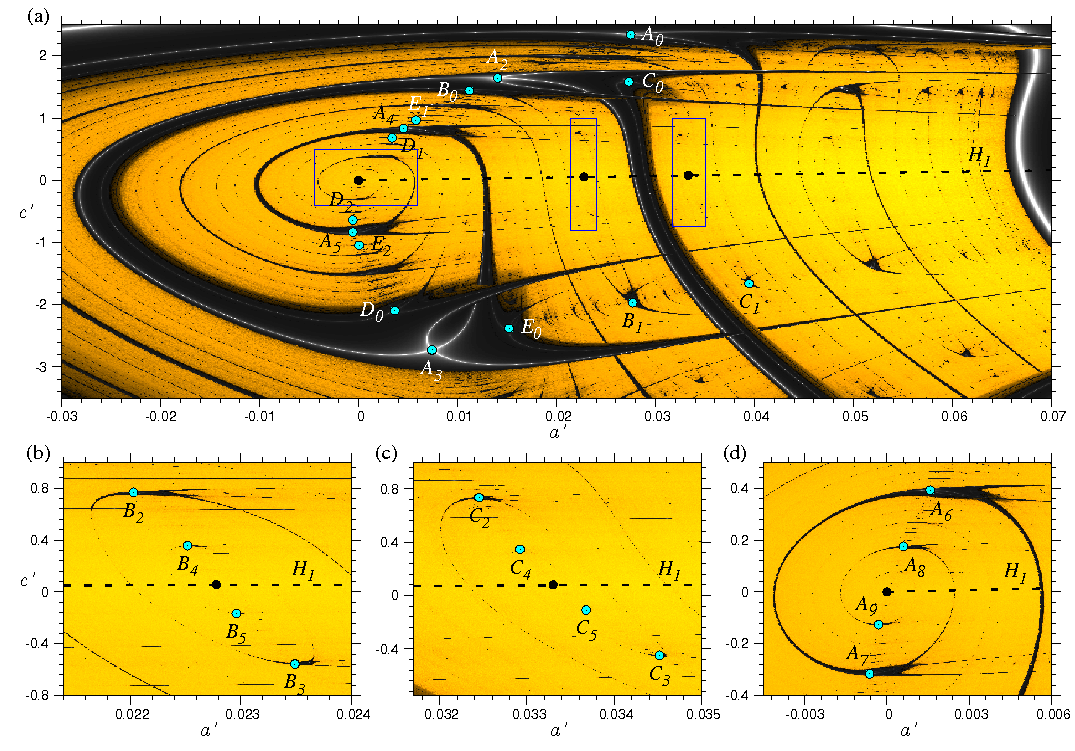
Figure 1: (Color online) (a) Parameter space $c^{\prime}\times a^{\prime}$. The phase space has an chaotic attractor for parameters in yellow and periodic for parameters in gray. The sets $A_{2}$ to $A_{5}$ are shrimps connected in a spiral way converging asymptotically to the onset of $H_{1}$ homoclinic curve (dashed line). $B$, $C$, $D$, and $E$ are shrimp families emerging by flip bifurcations in $A_{2}$ and $A_{3}$. The blue square regions are magnified in (b), (c), and (d). The black dots are the spiral focus and the blue dots indicate the shrimp positions.

For several smooth nonlinear maps and differential equations, stable periodic orbits and their dependence on the system control parameters are well known. The existence of these orbits can be properly visualized on a bi-dimensional parameter space, where generally we find periodic windows, i.e., continuous sets of parameters, embedded into chaotic regions, for which periodical orbits exist Fraser1982 ; Gallas1993 . There is an intricate periodic window, quite general in dynamical systems, whose local nature was explained in Fraser1982 ; Gallas1994 but the global features, despite the great number of studies Gaspard1984 ; Fraser1984 ; Mira1987 ; Ullmann1996 ; Baptista1997 ; Glass2001 ; Bonatto2005 ; Bonatto2007 ; Bonatto2008b ; Albuquerque2009 ; Albuquerque2009b ; Lorenz2008 ; Medeiros2010 , remain not well understood. For local and global features we mean typically qualities of an isolated and a multiple periodic windows, respectively. Recently, it has been found that these periodic windows, baptized shrimp Gallas1993 , are continuously connected along spirals emerging from in a homoclinic bifurcation point Feo2000 ; Bonatto2008c (set of parameters for which a bi-asymptotic curve, the homoclinic orbit, converges to a saddle-focus equilibrium point). These spiral structures were verified experimentally in Feo2003 ; Stoop2010 and are also observed in Gaspard1984 ; Veen2007 ; Albuquerque2008 .

However, in these researches the distribution of shrimps in the parameter space have not yet been clearly associated to any fundamental dynamical property. To accomplish this, we investigate the relation between the shrimps and the homoclinic curves in the parameter space Medrano2008 ; Medrano2010 . For the Rössler system, we present a new and remarkable two-parameter space scenery where from each shrimp emerge infinity spirals with focus in discrete points along of a homoclinic bifurcation curve (continuous parameter sets for which homoclinic orbits exist). Each spiral is composed by a shrimp family, i.e., infinite shrimps continuously connected in a spiral sequence. We show that, even the shrimps are a codimension-two phenomena (two parameters are necessary to obtain it), they are accumulating at the spiral focus following scaling laws predicted by the one-parameter space homoclinic theory Kuznetsov2004 . We also show that the reported period adding cascades observed in shrimps accumulations Bonatto2007 ; Bonatto2008b is a consequence of the spiral periodic windows approach to the homoclinic bifurcation point.

Recently was published a work Stoop2010 about scaling laws in a electronic homoclinic system where the authors associate scales of tangent bifurcation with the shrimp distribution. Here we discuss this issue in details and show that, in the two-parameter space, the scales measured in shrimps correspond to the distance between crosses of superstable periodic curves. Furthermore, we call the attention to the necessity of a rigorous prove of these scales in shrimp distributions which was done in Medrano2011 .

In section II we present the spiral scenery of periodic windows, in III we show the scaling laws concerning its distribution and periodicity, and in section IV we present the conclusions.

II Shrimp distributions

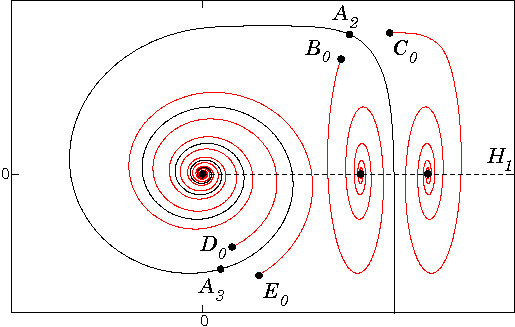
Figure 2: (Color online) Schematic scenery. Spiral in black corresponds to family $A$. In red are spirals emerging from shrimps $A_{2}$ and $A_{3}$. The dashed line is the $H_{1}$ homoclinic bifurcation. The dots along $H_{1}$ are the spiral focus points while the points in the spirals represent the crosses of superstables of $A_{2}$, $A_{3}$, $B_{0}$, $C_{0}$, $D_{0}$, and $E_{0}$.

We consider the homoclinic Rössler system given by

$$\begin{split}\dot{x}&=-y-z\\ \dot{y}&=x+ay\\ \dot{z}&=bx-cz+xz,\end{split}$$ (1)

where we fix $b=0.3$ and analyze the parameter space $c^{\prime}\times a^{\prime}$, where $a=a^{\prime}\sin(\theta)+c^{\prime}\cos(\theta)+a_{0}$ and $c=a^{\prime}\cos(\theta)-c^{\prime}\sin(\theta)+c_{0}$ with $a_{0}=0.3301$, $c_{0}=4.9305$, and $\theta=88.8^{\circ}$. For the region investigated (Fig. 1) the origin phase space ($P_{0}$) is a saddle-focus and the eigenvalues of Eqs. (1) Jacobian matrix evaluated at $P_{0}$ are $\lambda_{1,2}=\rho\pm i\omega$ and $\lambda_{3}=\lambda$, where $\lambda$, $\rho$, and $\omega$ are $\mathbb{R}^{*}$.

Periodic and chaotic asymptotic solutions of Eqs. (1) are determined numerically by evaluating the largest nonzero Lyapunov exponent $l$. In Fig. 1, from black to white ($l<0$) the periodic orbits increase their stability: in black these orbits bifurcate ($l=0$) and in white they are superstable ($l$ achieve the most negative value). Otherwise, from black to yellow ($l>0$) the behavior is asymptotically chaotic. The structure labeled $A_{3}$ is a particular region of the parameter space where a typical periodic window, the shrimp, can be visualized. The big shadow region, from which extends four narrow antennae, is its central body and corresponds to the fundamental periodic window where is the fundamental periodic orbit of the shrimp Lorenz2008 . The central body is bordered by tangent bifurcations, where we find chaotic regions, and by flip bifurcations, where we find sequences of doubled periodic regions with similar shape to the central body. The white lines form the shrimp skeleton (parameters set where the periodic regions are around) and represent superstable periodic orbits with behavior strongly attractive. Note that, in the central body, there is a cross between two remarkable superstable curves (blue dots in Fig. 1). We consider this point as a shrimp position and localize it identifying these intersections. In this sense, shrimps are codimensio-two structures.

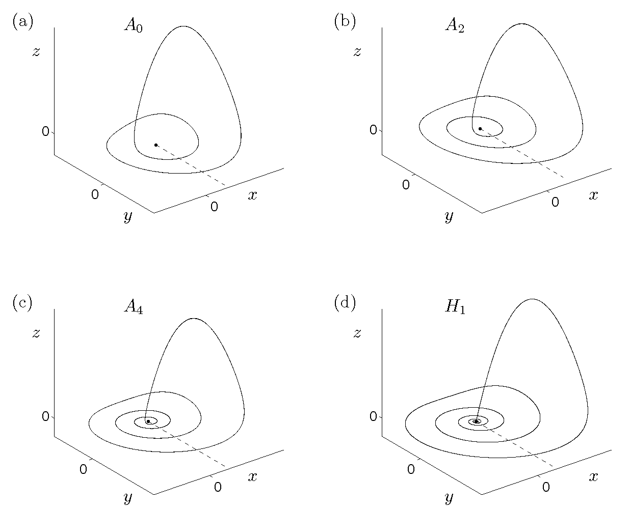
Figure 3: Period adding of $A$ shrimp family. The periodic trajectories cross the Poincaré section (dashed lines) two, three, four, and infinity times from (a) to (d), respectively.

To obtain the parameter sets of the homoclinic bifurcation $H_{1}$ associated with the saddle-focus point $P_{0}$, we determine numerically the parameters for which the stable and unstable manifolds of $P_{0}$ merge constituting a homoclinic orbit (To obtain homoclinic orbits in piecewise systems, see Ref. Medrano2003 ). The labels $A$, $B$, $C$, $D$, and $E$, in Fig. 1, indicate different shrimp families associated with $H_{1}$. Note that, in each family, shrimps are continuously connected along a spiral sequence around a homoclinic bifurcation point [Typically, two antennae of each shrimp central body is connected with the previous and the next shrimp and the other two antennae connect the shrimp to the divergence region ($a^{\prime}>0.2$)]. The index $i$, in the label families, indicates the element of these sequence. The first shrimp of the sequence is indexed by $i=1$, the second by $i=2$, and so on. The index $i=0$ indicates the structure that connect different families. Thus, $B_{0}$ connect family $A$ with family $B$. Furthermore, excluding the central body of $A_{2}$, for example, $B_{0}$ has the same features that characterize family $B$.

We observe that each shrimp generates many others spiral sequences by flip bifurcations. The central bodies of $A_{2}$ and $A_{3}$, in Fig. 1(a), bifurcate in $B_{0}$, $C_{0}$, $D_{0}$, and $E_{0}$, which connect the family $A$ with the families $B$, $C$, $D$, and $E$. The family $B$ converges to the region close the point ($a^{\prime}$ = 0.0228, $c^{\prime}$ = 0.0550) in an anti-clockwise direction and the family $C$ converges to the region close the point ($a^{\prime}$ = 0.0333, $c^{\prime}$ = 0.0800) in a clockwise direction. Both focus seems to be along the $H_{1}$ homoclinic bifurcation curve [see magnifications in Figs. 1(b) and (c)]. The families $A$, $D$ and $E$ converge to the $H_{1}$ onset point (0,0) [see Figs. 1(a) and (d)]. The schematic scenery is shown in Fig. 2. As far we could check, the same is observed in any element of any family suggesting the existence of a fractal structure of spiral self-replications converging asymptotically to the homoclinic bifurcation curve. Moreover, we identify shrimps concentrated in two sets, between the two shrimp antennae that converge to the divergence region (as $B$ and $C$ families), and between two shrimps, $i$ and $i+2$, of the same family (as $D$ and $E$ families).

With respect the trajectory behavior, following continuously a shrimp spiral sequence, we observe that the orbit time-period grows smoothly tending to infinity close the homoclinic orbit. So that, the fundamental periodic orbit add one cycle from $i$-shrimp to the $(i+2)$-shrimp forming a period adding cascade accumulating into the $H_{1}$ curve, as shown in Figs. 3 (a)-(d). The period adding can be identified considering a flat Poincaré section in $x=0$ with $y<0$ close to the plan $xy$ (represented by the dashed lines). The orbits cross the Poincaré section two times in (a), three times in (b), and four times in (c). The homoclinic orbit $H_{1}$ has infinite cycles in (d). Note that here we considered $A_{0}$ as a shrimp as discussed before.

III Scaling laws for shrimp distributions

Next we analyse our numerical results presented in the last section from the homoclinic theory described by Shilnikov theorem. We focus in the characterization of the two-parameter shrimp structures from these one-parameter theory.

Shilnikov theorem can be applied to systems which saddle-focus equilibrium point have homoclinic orbits ($\Gamma$) solutions and, in its normal form, can be represented by

$$\begin{split}\dot{x^{\prime}}&=\rho x^{\prime}-\omega y^{\prime}+O(x^{\prime},y^{\prime},z^{\prime})\\ \dot{y^{\prime}}&=\omega x^{\prime}+\rho y^{\prime}+P(x^{\prime},y^{\prime},z^{\prime})\\ \dot{z^{\prime}}&=-\lambda z^{\prime}+Q(x^{\prime},y^{\prime},z^{\prime}),\end{split}$$ (2)

where $O$, $P$, and $Q$ are analytic functions with $\dot{O}(\vec{x}^{\prime})=\dot{P}(\vec{x}^{\prime})=\dot{Q}(\vec{x}^{\prime})=0$, for the equilibrium saddle-focus point $\vec{x}^{\prime}=0$, and $\lambda$, $\rho$, and $\omega$ are $\mathbb{R}_{+}^{*}$.

If the saddle-focus form $\Gamma$ with saddle index $\nu<1/2$ ($\nu=\rho/\lambda$), the Shilnikov Theorem shows that, close to $\Gamma$, in a one-parameter space, there are infinite countable sets of periodic and homoclinic bifurcations accumulating into $\Gamma$, namely: (I) Stable periodic solutions emerge distributed as $S_{p}=\lim_{i\to\infty}(\mu_{i+1}/\mu_{i})=\exp{-(\pi\rho/\omega)}$ where $\mu_{i}$ and $\mu_{i+1}$ are two consecutive tangent bifurcation parameters Kuznetsov2004 ; Glendinning1984 ; Gaspard1984 . The period difference between two consecutive periodic orbits is $\Delta T=\lim_{i\to\infty}(T_{i+1}-T_{i})=\pi/\omega$, where $T_{i}$ is the period of the $i$-periodic orbit; (II) Infinite classes of homoclinic orbit, characterized by similar orbits, called secondary homoclinic orbits [double-pulse ($\Gamma_{2}$), triple-pulse ($\Gamma_{3}$), and $n$-pulse ($\Gamma_{n}$)] are distributed following $S_{\Gamma_{n}}=\lim_{i\to\infty}(\mu^{\prime}_{i+1}/\mu^{\prime}_{i})=\exp{-(\pi\lambda/\omega)}$, where $\mu^{\prime}_{i}$ and $\mu^{\prime}_{i+1}$ are two consecutive homoclinic bifurcation parameters of $\Gamma_{n}$ Medrano2005 . The limit $i=\infty$ is related with the primary single-pulse ($\Gamma_{1}$).

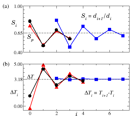
Figure 4: (Color online) (a) and (b) show, respectively, measure of distribution and difference time-period scalings of shrimps. The dashed lines are the theoretical values, $S_{p}=0.6498$ and $\Delta T=3.1840$, in the limit $i\to\infty$, of the family $A$. The symbols square, triangle, and circle are respect families $A$, $B$, and $C$.

To associate the shrimps with this theory, we verify these scaling laws in our numerical simulation. For the family $A$, the homoclinic orbit parameter is $(a^{\prime}_{\infty},c^{\prime}_{\infty})=(0,0)$ for which the eigenvalues calculated at the fixed point $P_{0}$ are $\lambda_{1,2}=0.1354\pm i0.9867$ and $\lambda_{3}=-4.8713$. Thus, the scaling laws are $S_{p}=0.6498$, $\Delta T=3.1840$, and $S_{\Gamma}\thickapprox 2.10^{-7}$. To measure numerically the periodic orbit scaling $S_{p}$, we define $S_{i}=d_{i+1}/d_{i}$, with $d_{i}=[(\tilde{a}_{i+1}^{\prime}-\tilde{a}_{i}^{\prime})^{2}+(\tilde{c}_{i+1}^{\prime}-\tilde{c}_{i}^{\prime})^{2}]^{1/2}$, where $(\tilde{a}_{i}^{\prime},\tilde{c}_{i}^{\prime})$ is an intersection point between two superstable curves as defined before the $i$-shrimp position. The measured $S_{i}$ for the shrimp family $A$ converges quickly to the theoretical scaling parameter $S_{p}$ as shown in Fig. 4(a) (curve with square symbol). Figure 4(b) shows that the measured time-period differences $\Delta T_{i}=T_{i+1}-T_{i}$ also converge quickly to the theoretical scaling $\Delta T$. Thus, in the limit $i\to\infty$, the period difference between $A_{i}$ and $A_{i+2}$ is $2\pi/\omega=6.3681$. This interval time corresponds to one periodic orbit revolution close to the unstable manifold (plan $xy$) and explains the period adding phenomenon in homoclinic systems. It suggests that similar mechanism can explain the period adding in other systems. For the family $B$, we consider $(a^{\prime}_{\infty},c^{\prime}_{\infty})=(0.0228,0.0550)$. The eigenvalues calculated at $P_{0}$ are $\lambda_{1,2}=0.1524\pm i0.9831$ and $\lambda_{3}=-4.7799$. Thus, the scaling laws are $S_{p}=0.6144$, $\Delta T=3.1956$, and $S_{\Gamma}\thickapprox 2.10^{-7}$, similarly to the family $A$. And, for the family $C$, $(a^{\prime}_{\infty},c^{\prime}_{\infty})=(0.0333,0.0800)$, $\lambda_{1,2}=0.1522\pm i0.9831$ and $\lambda_{3}=-4.7910$ with $S_{p}=0.6148$, $\Delta T=3.1955$, and $S_{\Gamma}\thickapprox 2.10^{-7}$. The scalings $S_{i}$ and $\Delta T_{i}$ of $B$ and $C$ families are in agreement to the theoretical estimated $S_{p}$ and $\Delta T$ as shown in Fig. 4(a) and (b) (triangle and circle symbols for $B$ and $C$ families, respectively). Although the homoclinic scaling law parameters is very low for being verified numerically, we have observed the existence of many different bifurcations $H_{n}$ close to the primary $H_{1}$ homoclinic curve parameter. The scalings measured of families $D$ and $E$ have values very similar to the family $A$ and it was omitted in Fig. 4.

We emphasize that it is not expected that the scaling laws here considered match with the shrimps scalings, since shrimps are a codimension-two phenomena. Our results suggest strongly that shrimps are distributed along lines in regions close to the homoclinic orbit bifurcation [See Figs. 1 (b)-(d)].

IV Conclusions

We used the knowledge of homoclinic orbits distribution in the bi-dimensional parameter space to explain the distribution of periodic windows in this space. We found infinite periodic structures with spiral shape distributed along the homoclinic bifurcation curve $H_{1}$. Each spiral has two extremities: one is a point in $H_{1}$, which is its focus, and the other is a shrimp. In the other side, from each shrimp derive infinite spirals with different focus along $H_{1}$. Thus, the spiral are composed by infinite shrimps, which compose infinite spirals which have infinite shrimps which compose infinite spirals and son on. This characterize the fractality of this scenery of spirals.

It is worth to mention that, excluding family $A$, each spiral is composed by a family of shrimps that, close the $H_{1}$ curve, the shape of its orbit in the phase space approaches the shape of an secondary homoclinic orbit $\Gamma_{n}$ (also called subsidiary homoclinic orbit). It suggest that the real focus of each spiral is a point close $H_{1}$ where is formed a $\Gamma_{n}$ orbit. As discussed before, the classes of homoclinic orbit are organized close $H_{1}$ following the scale $S_{\Gamma_{n}}$. Thus we argue that the spiral distribution in the parameter space should follows the scale $S_{\Gamma_{n}}$.

We have also identified properties of the homoclinic theory in the shrimps organization. We notice that this result is not expected since the homoclinic scalings are valid just in a one-parameter space and shrimps are two-parameter structures. It indicates that shrimps, close to the homoclinic bifurcation, are organized along a line that intersects $H_{1}$. The analytical prove of this is merit of investigation Medrano2011 .

Acknowledgments

We would like to thank Dr. Adilson E. Motter for important comments and suggestions about this paper, Dr. Manuel A. Matías for helpful discussions about bifurcation theory and Prof. Jason Gallas for previous discussions about shrimp properties. This research has a financial support of FAPESP and CNPq.

References

- (1) S. Fraser, R. Kapral, Phys. Rev. A 25 (1982) 3223.
- (2) J. A. C. Gallas, Phys. Rev. Lett. 70 (1993) 2714.
- (3) J. A. C. Gallas, Physica A 202 (1994) 196.
- (4) P. Gaspard, R. Kapral, G. Nicolis, J. Stat. Phys. 35 (1984) 697.
- (5) S. Fraser, R. Kapral, Phys. Rev. A 30 (1984) 1017.
- (6) C. Mira, Chaotic dynamics, World Scientific, Singapore, 1987.
- (7) K. Ullmann, I. L. Caldas, Chaos, Solitons and Fractals 7 (1996) 1913.
- (8) M. S. Baptista, I. L. Caldas, Int. J. Bifurcation Chaos 7 (1997) 447.
- (9) L. Glass, Nature 410 (2001) 277.
- (10) C. Bonatto, J. C. Garreau, J. A. C. Gallas, Phys. Rev. Lett. 95 (2005) 143905.
- (11) C. Bonatto, J. A. C. Gallas, Phys. Rev. E 75 (2007) 055204.
- (12) C. Bonatto, J. A. C. Gallas, Philos. Trans. R. Soc. A 366 (2008) 505.
- (13) O. C. D. Cardoso, H. A. Albuquerque, R. M. Rubinger, Phys. Lett. A 373 (2009) 2050.
- (14) H. A. Albuquerque, P. C. Rech, Int. J. Bifurcation Chaos 19 (2009) 1351.
- (15) E. N. Lorenz, Physica D 237 (2008) 1689.
- (16) E. S. Medeiros, S. L. T. de Souza, R. O. Medrano-T, I. L. Caldas, Phys. Lett. A 374 (2010) 2628.
- (17) O. Feo, G. M. Maggio, M. P. Kennedy, Int. J. Bifurcation Chaos 10 (2000) 935.
- (18) C. Bonatto, J. A. C. Gallas, Phys. Rev. Lett. 101 (2008) 054101.
- (19) O. De Feo, G. M. Maggio, Int. J. Bifurcation Chaos 13 (2003) 2917.
- (20) R. Stoop, P. Benner, Y. Uwate, Phys. Rev. Lett. 105 (2010) 074102.
- (21) L. van Veen,D. Liley, Phys. Rev. Lett. 97 (2007) 208101.
- (22) H. A. Albuquerque, R. M. Rubinger, P. C. Rech, Phys. Lett. A 372 (2008) 4793.
- (23) R. O. Medrano-T, COMPLEX SYSTEMS 2008, http://www.lac.inpe.br/WSACS/programme.jsp, 2008.
- (24) R. O. Medrano-T, I. L. Caldas, Dynamics Days South America 2010, http://urlib.net/sid.inpe.br/mtc-m19@80/2010/08.11.01.46, 2010.
- (25) Y. A. Kuznetsov, Elements of applied bifurcation theory, Springer, United States of America, 2004.
- (26) R. O. Medrano-T, I. L. Caldas (in preparation).
- (27) R. O. Medrano-T, M. S. Baptista, I. L. Caldas, Physica D 186 (2003) 133.
- (28) P. Glendinning, C. Sparrow, J. Stat. Phys. 35 (1984) 645.
- (29) R. O. Medrano-T, M. S. Baptista, I. L. Caldas, Chaos 15 (2005) 033112.