Slepton Mass Matrices, $\mu\rightarrow e\gamma$ Decay and EDM in SUSY $S_{4}$ Flavor Model

1 Introduction

Recent experiments of the neutrino oscillation go into a new phase of precise determination of mixing angles and mass squared differences  [1, 2, 3, 4], which indicate the tri-bimaximal mixing for three flavors in the lepton sector [5, 6, 7, 8]. These large mixing angles are completely different from the quark mixing ones. Therefore, there appear many researches to find a natural model that leads to the mass spectrum and mixing of quarks and leptons. The flavor symmetry is expected to explain them. In particular, the non-Abelian discrete symmetry of flavors [9] has been studied intensively in the quark and lepton sectors. Actually, the tri-bimaximal mixing of leptons has been at first understood based on the non-Abelian finite group $A_{4}$ [10, 11, 12, 13, 14]. Until now, much progress has been made in the theoretical and phenomenological analysis of $A_{4}$ flavor model  [15]-[75]. The other attractive candidate of the flavor symmetry is the $S_{4}$ symmetry, which was used for the neutrino masses and the neutrino flavor mixing  [76, 77, 78, 79]. The exact tri-bimaximal neutrino mixing is realized in $S_{4}$ flavor models [80, 81, 82, 83, 84, 85, 86]. Many studies in the $S_{4}$ flavor model have been presented for quarks as well as leptons  [87]-[103]. Some works attempt to unify the quark and lepton sectors toward a grand unified theory in the framework of the $S_{4}$ flavor symmetry [88, 89, 90], however, quark mixing angles were not predicted clearly.

Recently, $S_{4}$ flavor models to unify quarks and leptons have been proposed in the framework of the $SU(5)$ SUSY GUT  [82] or $SO(10)$ SUSY GUT [104, 105]. There also appeared the $S_{4}$ flavor model in $SU(5)$ SUSY GUT  [106, 107, 108] and the Pati-Salam SUSY GUT [109, 110], taking account of the next-to-leading order of mass operators. These unified models seem to explain both mixing of quarks and leptons.

Since many flavor models have been proposed, it is important to study how to test them. The flavor symmetry in the framework of SUSY controls the slepton and squark mass matrices as well as the quark and lepton ones. For example, the predicted slepton mass matrices reflect structures of the charged lepton mass matrix. Therefore, the slepton mass matrices provide us an important test for the flavor symmetry.

Our $S_{4}$ flavor model [108] is an attractive one because it gives the proper quark flavor mixing angles as well as the tri-bimaximal mixing of neutrino flavors. Especially, the Cabibbo angle is predicted to be $15^{\circ}$ due to $S_{4}$ Clebsch-Gordan coefficients in the leading order. Including the next-to-leading corrections of the $S_{4}$ symmetry, the predicted Cabibbo angle is completely consistent with the observed one.

In our $S_{4}$ flavor model, three generations of $\overline{5}$-plets in $SU(5)$ are assigned to ${\bf 3}$ of $S_{4}$ while the first and second generations of $10$-plets in $SU(5)$ are assigned to ${\bf 2}$ of $S_{4}$, and the third generation of $10$-plet is assigned to ${\bf 1}$ of $S_{4}$. These assignments of $S_{4}$ for $\overline{5}$ and $10$ lead to the completely different structure of quark and lepton mass matrices. Right-handed neutrinos, which are $SU(5)$ gauge singlets, are also assigned to ${\bf 2}$ for the first and second generations, and ${\bf 1}^{\prime}$ for the third generation. These assignments realize the tri-bimaximal mixing of neutrino flavors.

We discuss slepton mass matrices in our $S_{4}$ flavor model by considering the gravity mediation within the framework of supergravity theory. We estimate the SUSY breaking in the slepton mass matrices by taking account of the next-to-leading $S_{4}$ invariant mass operators. Then, we can predict the lepton flavor violation (LFV), e.g., the $\mu\rightarrow e+\gamma$ decay. A similar study of the LFV has been presented in the $A_{4}$ flavor model [111]. Slepton mass matrices also give the electric dipole moment (EDM) of the lepton [112, 113], which has not been discussed in flavor models with the non-Abelian discrete symmetry. We predict the EDM of the electron versus the $\mu\rightarrow e+\gamma$ decay ratio, which are important to study the SUSY sector comprehensively [114, 115, 116].

In section 2, we summarize briefly the $S_{4}\times Z_{4}\times U(1)_{FN}$ flavor model of quarks and leptons in $SU(5)$ SUSY GUT including the higher dimensional mass operators. In section 3, the slepton mass matrices are discussed precisely. The numerical predictions of LFV processes and lepton EDM’s are presented in section 4. Section 5 is devoted to the summary. The multiplication rule of $S_{4}$ is presented in Appendix.

2 Overview of $S_{4}$ flavor model with $SU(5)$ SUSY GUT

In this section, we summarize our $S_{4}$ flavor model [108] to unify quarks and leptons in the framework of the $SU(5)$ SUSY GUT. The $S_{4}$ group has 24 distinct elements and irreducible representations ${\bf 1},~{}{\bf 1}^{\prime},~{}{\bf 2},~{}{\bf 3}$, and ${\bf 3}^{\prime}$, which are assigned for each $SU(5)$ representation.

	$(T_{1},T_{2})$	$T_{3}$	$(F_{1},F_{2},F_{3})$	$(N_{e}^{c},N_{\mu}^{c})$	$N_{\tau}^{c}$	$H_{5}$	$H_{\bar{5}}$	$H_{45}$	$\Theta$
$SU(5)$	$10$	$10$	$\bar{5}$	$1$	$1$	$5$	$\bar{5}$	$45$	$1$
$S_{4}$	$\bf 2$	$\bf 1$	$\bf 3$	$\bf 2$	${\bf 1}^{\prime}$	$\bf 1$	$\bf 1$	$\bf 1$	$\bf 1$
$Z_{4}$	$-i$	$-1$	$i$	$1$	$1$	$1$	$1$	$-1$	$1$
$U(1)_{FN}$	$1$	0	0	$1$	0	0	0	0	$-1$

	$(\chi_{1},\chi_{2})$	$(\chi_{3},\chi_{4})$	$(\chi_{5},\chi_{6},\chi_{7})$	$(\chi_{8},\chi_{9},\chi_{10})$	$(\chi_{11},\chi_{12},\chi_{13})$	$\chi_{14}$	$(\chi_{15},\chi_{16},\chi_{17})$
$SU(5)$	$1$	$1$	$1$	$1$	$1$	$1$	$1$
$S_{4}$	$\bf 2$	$\bf 2$	${\bf 3}^{\prime}$	$\bf 3$	$\bf 3$	$\bf 1$	$\bf 3$
$Z_{4}$	$-i$	$1$	$-i$	$-1$	$i$	$i$	$-1$
$U(1)_{FN}$	$-1$	$-2$	0	0	0	$-1$	$-z$

Table 1: Assignments of $SU(5)$, $S_{4}$, $Z_{4}$, and $U(1)_{FN}$ representations.

In $SU(5)$, matter fields are unified into $10$ and $\bar{5}$ dimensional representations. Three generations of $\bar{5}$, which are denoted by $F_{i}~{}(i=1,2,3)$, are assigned to $\bf 3$ of $S_{4}$. On the other hand, the third generation of the $10$-dimensional representation, $T_{3}$, is assigned to $\bf 1$ of $S_{4}$, and the first and second generations of $10$, $(T_{1},T_{2})$, are assigned to $\bf 2$ of $S_{4}$, respectively. Right-handed neutrinos, which are $SU(5)$ gauge singlets, are also assigned to ${\bf 2}$ for the first and second generations, $(N_{e}^{c},N_{\mu}^{c})$, and ${\bf 1}^{\prime}$ for the third one, $N_{\tau}^{c}$. The $5$-dimensional, $\bar{5}$-dimensional, and $45$-dimensional Higgs of $SU(5)$, $H_{5}$, $H_{\bar{5}}$, and $H_{45}$ are assigned to $\bf 1$ of $S_{4}$. In order to obtain desired mass matrices, we introduce $SU(5)$ gauge singlets $\chi_{i}$, so called flavons, which couple to quarks and leptons.

The $Z_{4}$ symmetry is added to obtain relevant couplings. The Froggatt-Nielsen mechanism [117] is introduced to get the natural hierarchy among quark and lepton masses, as an additional $U(1)_{FN}$ flavor symmetry, where $\Theta$ denotes the Froggatt-Nielsen flavon. The particle assignments of $SU(5)$, $S_{4}$, $Z_{4}$, and $U(1)_{FN}$ are presented in Table 1.

The couplings of flavons are restricted as follows. In the leading order, $(\chi_{3},\chi_{4})$ are coupled with the right-handed Majorana neutrino sector, $(\chi_{5},\chi_{6},\chi_{7})$ are coupled with the Dirac neutrino sector, $(\chi_{8},\chi_{9},\chi_{10})$ and $(\chi_{11},\chi_{12},\chi_{13})$ are coupled with the charged lepton and down-type quark sectors. In the next-to-leading order, $(\chi_{1},\chi_{2})$ are coupled with the up-type quark sector, and $\chi_{14}$ contributes to the charged lepton and down-type quark sectors, and then the mass ratio of the electron and down quark is reproduced properly. The $S_{4}$ triplet $(\chi_{15},\chi_{16},\chi_{17})$ does not couple with quarks and leptons directly due to $U(1)_{FN}$ as far as $z\gg 1$, but couples with other flavons to give alignments of vacuum expectation values (VEV’s) as discussed later.

Our model predicts the quark mixing as well as the tri-bimaximal mixing of leptons. Especially, the Cabibbo angle is predicted to be $15^{\circ}$ in the leading order. The model is consistent with the observed CKM mixing angles and $CP$ violation as well as the non-vanishing $U_{e3}$ of the neutrino flavor mixing.

Let us write down the superpotential respecting $S_{4}$, $Z_{4}$ and $U(1)_{FN}$ symmetries in terms of the $S_{4}$ cutoff scale $\Lambda$, and the $U(1)_{FN}$ cutoff scale $\overline{\Lambda}$. In our calculation, both cutoff scales are taken as the GUT scale which is around $10^{16}$GeV. The $SU(5)$ invariant superpotential of the Yukawa sector up to the linear terms of $\chi_{i}$ ($i=1,\cdots,13$) is given as

$$w =y_{1}^{u}(T_{1},T_{2})\otimes T_{3}\otimes(\chi_{1},\chi_{2})\otimes H_{5}/\Lambda+y_{2}^{u}T_{3}\otimes T_{3}\otimes H_{5}$$

$$\ +y_{1}^{N}(N_{e}^{c},N_{\mu}^{c})\otimes(N_{e}^{c},N_{\mu}^{c})\otimes\Theta^{2}/\bar{\Lambda}$$

$$\ +y_{2}^{N}(N_{e}^{c},N_{\mu}^{c})\otimes(N_{e}^{c},N_{\mu}^{c})\otimes(\chi_{3},\chi_{4})+MN_{\tau}^{c}\otimes N_{\tau}^{c}$$

$$\ +y_{1}^{D}(N_{e}^{c},N_{\mu}^{c})\otimes(F_{1},F_{2},F_{3})\otimes(\chi_{5},\chi_{6},\chi_{7})\otimes H_{5}\otimes\Theta/(\Lambda\bar{\Lambda})$$

$$\ +y_{2}^{D}N_{\tau}^{c}\otimes(F_{1},F_{2},F_{3})\otimes(\chi_{5},\chi_{6},\chi_{7})\otimes H_{5}/\Lambda$$

$$\ +y_{1}(F_{1},F_{2},F_{3})\otimes(T_{1},T_{2})\otimes(\chi_{8},\chi_{9},\chi_{10})\otimes H_{45}\otimes\Theta/(\Lambda\bar{\Lambda})$$

$$\ +y_{2}(F_{1},F_{2},F_{3})\otimes T_{3}\otimes(\chi_{11},\chi_{12},\chi_{13})\otimes H_{\bar{5}}/\Lambda,$$ (1)

where $y_{1}^{u}$, $y_{2}^{u}$, $y_{1}^{N}$, $y_{2}^{N}$, $y_{1}^{D}$, $y_{2}^{D}$, $y_{1}$, and $y_{2}$ are Yukawa couplings of order one, and $M$ is the right-handed Majorana mass, which is taken to be $10^{12}$GeV in our calculation. We can discuss the feature of the quark and lepton mass matrices and flavor mixing based on this superpotential by using the $S_{4}$ multiplication rule in Appendix.

We require vacuum alignments for the VEV’s of flavons in order to get desired quarks and leptons mass matrices. The alignment depends on the structure of the scalar potential which is constructed by adding driving fields $\chi_{1}^{0}$, $\chi_{2}^{0}$, $\chi_{3}^{0}$ and $(\chi_{4}^{0},\chi_{5}^{0})$ with having $U(1)_{R}$ charge two as shown in Table 2. Matter fields ($T_{i}$, $F_{i}$, and $N_{i}$) are assigned to $U(1)_{R}$ charge one and Higgs, flavons are assigned to zero. A continuous $U(1)_{R}$ symmetry contains the usual R-parity as a subgroup.

The superpotential of the scalar sector including driving fields is given by

$$w^{\prime} =\kappa_{1}\left(\chi_{1},\chi_{2}\right)\otimes\left(\chi_{1},\chi_{2}\right)\otimes\left(\chi_{3},\chi_{4}\right)\otimes\chi_{1}^{0}/\Lambda$$

$$\ +\eta_{1}\left(\chi_{8},\chi_{9},\chi_{10}\right)\otimes\left(\chi_{11},\chi_{12},\chi_{13}\right)\otimes\chi_{2}^{0}$$

$$\ +\eta_{2}\left(\chi_{1},\chi_{2}\right)\otimes\left(\chi_{1},\chi_{2}\right)\otimes\chi_{3}^{0}+\eta_{3}\chi_{14}\otimes\chi_{14}\otimes\chi_{3}^{0}$$

$$\ +\eta_{4}\left(\chi_{5},\chi_{6},\chi_{7}\right)\otimes\left(\chi_{15},\chi_{16},\chi_{17}\right)\otimes\left(\chi_{4}^{0},\chi_{5}^{0}\right),$$ (2)

where $\kappa_{1}$ and $\eta_{i}$ ($i=1$–4) are coupling constants of order one. It gives the scalar potential

$$V =\left|\frac{\kappa_{1}}{\Lambda}\left[2\chi_{1}\chi_{2}\chi_{3}+\left(\chi_{1}^{2}-\chi_{2}^{2}\right)\chi_{4}\right]\right|^{2}+\left|\eta_{1}\left(\chi_{8}\chi_{11}+\chi_{9}\chi_{12}+\chi_{10}\chi_{13}\right)\right|^{2}$$

$$\ +\left|\eta_{2}(\chi_{1}^{2}+\chi_{2}^{2})+\eta_{3}\chi_{14}^{2}\right|^{2}+\left|\frac{1}{\sqrt{2}}\eta_{4}\left(\chi_{6}\chi_{16}-\chi_{7}\chi_{17}\right)\right|^{2}$$

$$\ +\left|\frac{1}{\sqrt{6}}\eta_{4}\left(-2\chi_{5}\chi_{15}+\chi_{6}\chi_{16}+\chi_{7}\chi_{17}\right)\right|^{2}\ .$$ (3)

Therefore, conditions to realize the potential minimum ($V=0$) are given as

$$(\chi_{1},\chi_{2})=(1,1),\quad(\chi_{3},\chi_{4})=(0,1),\quad(\chi_{5},\chi_{6},\chi_{7})=(1,1,1),\quad(\chi_{8},\chi_{9},\chi_{10})=(0,1,0),$$

$$(\chi_{11},\chi_{12},\chi_{13})=(0,0,1),\quad\chi_{14}^{2}=-\frac{2\eta_{2}}{\eta_{3}}\chi_{1}^{2},\quad(\chi_{15},\chi_{16},\chi_{17})=(1,1,1),$$ (4)

where these magnitudes are given in arbitrary units. Hereafter, we suppose these gauge-singlet scalars develop VEV’s by denoting $\langle\chi_{i}\rangle=a_{i}\Lambda$, where $a_{i}$’s are given to be same order as shown in section 4.

Denoting Higgs doublets as $h_{u}$ and $h_{d}$, we take VEV’s of following scalars by

$$\langle h_{u}\rangle=v_{u},\quad\langle h_{d}\rangle=v_{d},\quad\langle h_{45}\rangle=v_{45},\quad\langle\Theta\rangle=\theta,$$ (5)

which are supposed to be real. We define $\lambda=\theta/\Lambda$ to describe the Froggatt-Nielsen mechanism.

	$\chi_{1}^{0}$	$\chi_{2}^{0}$	$\chi_{3}^{0}$	$(\chi_{4}^{0},\chi_{5}^{0})$
$SU(5)$	$1$	$1$	$1$	$1$
$S_{4}$	$\bf 1$	$\bf 1$	$\bf 1$	$\bf 2$
$Z_{4}$	$-1$	$i$	$-1$	$-i$
$U(1)_{FN}$	$4$	$0$	$2$	$z$
$U(1)_{R}$	$2$	$2$	$2$	$2$

Table 2: Assignments of $SU(5)$, $S_{4}$, $Z_{4}$, and $U(1)_{FN}$ representations.

First we consider mass matrices of the lepton sector. Taking vacuum alignments in Eq. (4), the mass matrix of charged lepton becomes

$$M_{l}=\begin{pmatrix}0&-3y_{1}\lambda a_{9}v_{45}/\sqrt{2}&0\\ 0&-3y_{1}\lambda a_{9}v_{45}/\sqrt{6}&0\\ 0&0&y_{2}a_{13}v_{d}\end{pmatrix},$$ (6)

then, masses are given as

$$m_{e}^{2}=0\ ,\quad m_{\mu}^{2}=6|\bar{y}_{1}\lambda a_{9}|^{2}v_{d}^{2}\ ,\quad m_{\tau}^{2}=|y_{2}|^{2}a_{13}^{2}v_{d}^{2}\ .$$ (7)

In the same way, the right-handed Majorana mass matrix of neutrinos is given by

$$M_{N}=\begin{pmatrix}y_{1}^{N}\lambda^{2}\bar{\Lambda}+y_{2}^{N}a_{4}\Lambda&0&0\\ 0&y_{1}^{N}\lambda^{2}\bar{\Lambda}-y_{2}^{N}a_{4}\Lambda&0\\ 0&0&M\end{pmatrix},$$ (8)

and the Dirac mass matrix of neutrinos is

$$M_{D}=y_{1}^{D}\lambda v_{u}\begin{pmatrix}2a_{5}/\sqrt{6}&-a_{5}/\sqrt{6}&-a_{5}/\sqrt{6}\\ 0&a_{5}/\sqrt{2}&-a_{5}/\sqrt{2}\\ 0&0&0\end{pmatrix}+y_{2}^{D}v_{u}\begin{pmatrix}0&0&0\\ 0&0&0\\ a_{5}&a_{5}&a_{5}\end{pmatrix}.$$ (9)

By using the seesaw mechanism $M_{\nu}=M_{D}^{T}M_{N}^{-1}M_{D}$, the left-handed Majorana neutrino mass matrix is written as

$$M_{\nu}=\begin{pmatrix}a+\frac{2}{3}b&a-\frac{1}{3}b&a-\frac{1}{3}b\\ a-\frac{1}{3}b&a+\frac{1}{6}b+\frac{1}{2}c&a+\frac{1}{6}b-\frac{1}{2}c\\ a-\frac{1}{3}b&a+\frac{1}{6}b-\frac{1}{2}c&a+\frac{1}{6}b+\frac{1}{2}c\end{pmatrix},$$ (10)

where

$$a=\frac{(y_{2}^{D}a_{5}v_{u})^{2}}{M},\qquad b=\frac{(y_{1}^{D}a_{5}v_{u}\lambda)^{2}}{y_{1}^{N}\lambda^{2}\bar{\Lambda}+y_{2}^{N}a_{4}\Lambda},\qquad c=\frac{(y_{1}^{D}a_{5}v_{u}\lambda)^{2}}{y_{1}^{N}\lambda^{2}\bar{\Lambda}-y_{2}^{N}a_{4}\Lambda}.$$ (11)

It gives the tri-bimaximal mixing matrix $U_{\text{tri-bi}}$ and mass eigenvalues as follows:

$$U_{\text{tri-bi}}=\begin{pmatrix}\frac{2}{\sqrt{6}}&\frac{1}{\sqrt{3}}&0\\ -\frac{1}{\sqrt{6}}&\frac{1}{\sqrt{3}}&-\frac{1}{\sqrt{2}}\\ -\frac{1}{\sqrt{6}}&\frac{1}{\sqrt{3}}&\frac{1}{\sqrt{2}}\end{pmatrix},$$

$$m_{\nu_{1}}=b\ ,\qquad m_{\nu_{2}}=3a\ ,\qquad m_{\nu_{3}}=c\ .$$ (12)

The next-to-leading terms of the superpotential are important to predict the deviation from the tri-bimaximal mixing of leptons, especially, $U_{e3}$. The relevant superpotential in the charged lepton sector is given at the next-to-leading order as

$$\Delta w_{l} =y_{\Delta_{a}}(T_{1},T_{2})\otimes(F_{1},F_{2},F_{3})\otimes(\chi_{1},\chi_{2})\otimes(\chi_{11},\chi_{12},\chi_{13})\otimes H_{\bar{5}}/\Lambda^{2}$$

$$\ +y_{\Delta_{b}}(T_{1},T_{2})\otimes(F_{1},F_{2},F_{3})\otimes(\chi_{5},\chi_{6},\chi_{7})\otimes\chi_{14}\otimes H_{\bar{5}}/\Lambda^{2}$$

$$\ +y_{\Delta_{c}}(T_{1},T_{2})\otimes(F_{1},F_{2},F_{3})\otimes(\chi_{1},\chi_{2})\otimes(\chi_{5},\chi_{6},\chi_{7})\otimes H_{45}/\Lambda^{2}$$

$$\ +y_{\Delta_{d}}(T_{1},T_{2})\otimes(F_{1},F_{2},F_{3})\otimes(\chi_{11},\chi_{12},\chi_{13})\otimes\chi_{14}\otimes H_{45}/\Lambda^{2}$$

$$\ +y_{\Delta_{e}}T_{3}\otimes(F_{1},F_{2},F_{3})\otimes(\chi_{5},\chi_{6},\chi_{7})\otimes(\chi_{8},\chi_{9},\chi_{10})\otimes H_{\bar{5}}\otimes/\Lambda^{2}$$

$$\ +y_{\Delta_{f}}T_{3}\otimes(F_{1},F_{2},F_{3})\otimes(\chi_{8},\chi_{9},\chi_{10})\otimes(\chi_{11},\chi_{12},\chi_{13})\otimes H_{45}\otimes/\Lambda^{2}\ .$$ (13)

By using this superpotential, we obtain the charged lepton mass matrix as

$$M_{l}\simeq\begin{pmatrix}\epsilon_{11}&\frac{\sqrt{3}m_{\mu}}{2}+\epsilon_{12}&\epsilon_{13}\\ \epsilon_{21}&\frac{m_{\mu}}{2}+\epsilon_{22}&\epsilon_{23}\\ \epsilon_{31}&0&m_{\tau}+\epsilon_{33}\end{pmatrix},$$ (14)

where $m_{\mu}$ and $m_{\tau}$ are given in Eq. (7), and $\epsilon_{ij}$’s are calculated by using Eq. (13) to find

$$\epsilon_{11} =y_{\Delta_{b}}a_{5}a_{14}v_{d}-3\bar{y}_{\Delta_{c_{2}}}a_{1}a_{5}v_{d},$$

$$\epsilon_{12} =-\frac{1}{2}y_{\Delta_{b}}a_{5}a_{14}v_{d}+3\left[\frac{\sqrt{3}}{4}(\sqrt{3}-1)\bar{y}_{\Delta_{c_{1}}}-\frac{1}{4}(\sqrt{3}+1)\bar{y}_{\Delta_{c_{2}}}\right]a_{1}a_{5}v_{d},$$

$$\epsilon_{13} =\left[\left\{\frac{\sqrt{3}}{4}(\sqrt{3}-1)y_{\Delta_{a_{1}}}+\frac{1}{4}(\sqrt{3}+1)y_{\Delta_{a_{2}}}\right\}a_{1}a_{13}-\frac{1}{2}y_{\Delta_{b}}a_{5}a_{14}\right]v_{d}$$

$$\ -3\left[\left\{-\frac{\sqrt{3}}{4}(\sqrt{3}+1)\bar{y}_{\Delta_{c_{1}}}-\frac{1}{4}(\sqrt{3}-1)\bar{y}_{\Delta_{c_{2}}}\right\}a_{1}a_{5}+\frac{\sqrt{3}}{2}\bar{y}_{\Delta_{d}}a_{13}a_{14}\right]v_{d},$$

$$\epsilon_{21} =-3\bar{y}_{\Delta_{c_{1}}}a_{1}a_{5}v_{d},$$

$$\epsilon_{22} =\frac{\sqrt{3}}{2}y_{\Delta_{b}}a_{5}a_{14}v_{d}+3\left[\frac{1}{4}(\sqrt{3}-1)\bar{y}_{\Delta_{c_{1}}}+\frac{\sqrt{3}}{4}(\sqrt{3}+1)\bar{y}_{\Delta_{c_{2}}}\right]a_{1}a_{5}v_{d},$$

$$\epsilon_{23} =\left[\left\{-\frac{1}{4}(\sqrt{3}-1)y_{\Delta_{a_{1}}}+\frac{\sqrt{3}}{4}(\sqrt{3}+1)y_{\Delta_{a_{2}}}\right\}a_{1}a_{13}-\frac{\sqrt{3}}{2}y_{\Delta_{b}}a_{5}a_{14}\right]v_{d}$$

$$\ -3\left[\left\{\frac{1}{4}(\sqrt{3}+1)\bar{y}_{\Delta_{c_{1}}}-\frac{\sqrt{3}}{4}(\sqrt{3}-1)\bar{y}_{\Delta_{c_{2}}}\right\}a_{1}a_{5}-\frac{1}{2}\bar{y}_{\Delta_{d}}a_{13}a_{14}\right]v_{d},$$

$$\epsilon_{31} =-y_{\Delta_{e}}a_{5}a_{9}v_{d}-3\bar{y}_{\Delta_{f}}a_{9}a_{13}v_{d},$$

$$\epsilon_{33} =y_{\Delta_{e}}a_{5}a_{9}v_{d}.$$ (15)

Since $\epsilon_{ij}$’s are given as relevant linear combinations of $a_{k}a_{l}$’s and all $a_{i}^{\prime}s$ are the same order, these are expected to be the same order, assuming Yukawa couplings are of order one. Therefore, the magnitude of $\epsilon_{ij}$’s are denoted to be ${\cal O}(\tilde{a}^{2}v_{d})$, which is expected to be ${\cal O}(a_{i}^{2}v_{d})$. The charged lepton is diagonalized by the left-handed mixing matrix $U_{E}$ and the right-handed one $V_{E}$ as

$$V_{E}^{\dagger}M_{\ell}U_{E}=M_{\ell}^{\text{diag}},$$ (16)

where $M_{\ell}^{\text{diag}}$ is a diagonal matrix. These mixing matrices can be written by

$$\begin{split}V_{E}&=\begin{pmatrix}\cos 60^{\circ}&\sin 60^{\circ}&0\\ -\sin 60^{\circ}&\cos 60^{\circ}&0\\ 0&0&1\end{pmatrix}\times\begin{pmatrix}1&\frac{\tilde{a}^{2}}{\lambda^{2}}&\tilde{a}\\ -\frac{\tilde{a}^{2}}{\lambda^{2}}-\tilde{a}^{2}&1&\tilde{a}\\ -\tilde{a}+\frac{\tilde{a}^{3}}{\lambda^{2}}&-\tilde{a}-\frac{\tilde{a}^{3}}{\lambda^{2}}&1\end{pmatrix},\\ U_{E}&=\begin{pmatrix}1&\frac{\tilde{a}}{\lambda}&\tilde{a}\\ -\frac{\tilde{a}}{\lambda}-\tilde{a}^{2}&1&\tilde{a}\\ -\tilde{a}+\frac{\tilde{a}^{2}}{\lambda}&-\tilde{a}-\frac{\tilde{a}^{2}}{\lambda}&1\end{pmatrix}.\end{split}$$ (17)

Taking the next-to-leading order, the electron has non-zero mass, namely

$$m_{e}^{2} \simeq\frac{3}{2}\left(\frac{1}{6}\epsilon_{11}^{2}-\frac{1}{\sqrt{3}}\epsilon_{11}\epsilon_{21}+\frac{1}{2}\epsilon_{21}^{2}\right)\simeq{\cal O}(\tilde{a}^{4}v_{d}^{2}).$$ (18)

Next, the down-type quark mass matrix including the next-to-leading order is

$$M_{d}\simeq\begin{pmatrix}\bar{\epsilon}_{11}&\bar{\epsilon}_{21}&\bar{\epsilon}_{31}\\ \frac{\sqrt{3}m_{s}}{2}+\bar{\epsilon}_{12}&\frac{m_{s}}{2}+\bar{\epsilon}_{22}&\bar{\epsilon}_{32}\\ \bar{\epsilon}_{13}&\bar{\epsilon}_{23}&m_{b}+\bar{\epsilon}_{33}\end{pmatrix},$$ (19)

where $\bar{\epsilon}_{ij}$’s are given by replacing $\bar{y}_{\Delta_{i}}$ with $-\bar{y}_{\Delta_{i}}/3\ (i=c_{1},c_{2},d,f)$ in Eq. (15). Since the alignment $a_{1}=a_{2}$ is taken as in Eq. (4), the mass matrix of the up-type quarks is given as

$$M_{u}=v_{u}\begin{pmatrix}2y_{\Delta_{a_{1}}}^{u}a_{1}^{2}+y_{\Delta_{b}}^{u}a_{14}^{2}&y_{\Delta_{a_{2}}}^{u}a_{1}^{2}&y_{1}^{u}a_{1}\\ y_{\Delta_{a_{2}}}^{u}a_{1}^{2}&2y_{\Delta_{a_{1}}}^{u}a_{1}^{2}+y_{\Delta_{b}}^{u}a_{14}^{2}&y_{1}^{u}a_{1}\\ y_{1}^{u}a_{1}&y_{1}^{u}a_{1}&y_{2}^{u}+y_{\Delta_{c}}^{u}a_{9}^{2}\end{pmatrix}.$$ (20)

Therefore, the CKM matrix $V^{0}$ at the GUT scale can be written as

$$V^{0}=U_{u}^{\dagger}\begin{pmatrix}1&0&0\\ 0&e^{-i\rho}&0\\ 0&0&1\end{pmatrix}U_{d}\ ,$$ (21)

where the left-handed mixing matrix of the up quarks $U_{u}$ is given as

$$U_{u}=\begin{pmatrix}\cos 45^{\circ}&\sin 45^{\circ}&0\\ -\sin 45^{\circ}&\cos 45^{\circ}&0\\ 0&0&1\end{pmatrix}\begin{pmatrix}1&0&0\\ 0&r_{t}&r_{c}\\ 0&-r_{c}&r_{t}\end{pmatrix},$$ (22)

and the left-handed mixing matrix of the down quarks $U_{d}$ is given as

$$U_{d}=\begin{pmatrix}\cos 60^{\circ}&\sin 60^{\circ}&0\\ -\sin 60^{\circ}&\cos 60^{\circ}&0\\ 0&0&1\end{pmatrix}\begin{pmatrix}1&\theta_{12}^{d}&\theta_{13}^{d}\\ -\theta_{12}^{d}-\theta_{13}^{d}\theta_{23}^{d}&1&\theta_{23}^{d}\\ -\theta_{13}^{d}+\theta_{12}^{d}\theta_{23}^{d}&-\theta_{23}^{d}-\theta_{12}^{d}\theta_{13}^{d}&1\\ \end{pmatrix}.$$ (23)

Here, $r_{c}=\sqrt{m_{c}/(m_{c}+m_{t})}$, $r_{t}=\sqrt{m_{t}/(m_{c}+m_{t})}$, and the phase $\rho$ is an arbitrary parameter originating from complex Yukawa couplings. Magnitudes of $\theta_{ij}^{d}$ are given as

$$\theta_{12}^{d}=\mathcal{O}\left(\frac{m_{d}}{m_{s}}\right)=\mathcal{O}\left(0.05\right),\ \ \theta_{13}^{d}=\mathcal{O}\left(\frac{m_{d}}{m_{b}}\right)=\mathcal{O}\left(0.005\right),\$$

$$\theta_{23}^{d}=\mathcal{O}\left(\frac{m_{d}}{m_{b}}\right)=\mathcal{O}\left(0.005\right).$$ (24)

At the leading order, the Cabibbo angle is derived as $15^{\circ}$ and it can be naturally fitted to the observed value by including the next-to-leading order as follows:

$$V_{us}^{0} \simeq\theta_{12}^{d}\cos 15^{\circ}+\sin 15^{\circ}.$$ (25)

Magnitudes of $a_{i}=\langle\chi_{i}\rangle/\Lambda$ are determined by putting the quark and lepton masses, except for $a_{14}$, which appears at the next-to-leading order. These are given as

$$a_{3}=a_{8}=a_{10}=a_{11}=a_{12}=0,\qquad a_{1}=a_{2}\simeq\sqrt{\frac{m_{c}}{2\left|y_{\Delta_{a_{2}}}^{u}-\frac{{y_{1}^{u}}^{2}}{y_{2}^{u}}\right|v_{u}}}~{},$$

$$a_{4}=\frac{(y_{1}^{D}\lambda)^{2}(m_{3}-m_{1})m_{2}M}{6y_{2}^{N}{y_{2}^{D}}^{2}m_{1}m_{3}\Lambda},\qquad a_{5}=a_{6}=a_{7}=\frac{\sqrt{m_{2}M}}{\sqrt{3}y_{2}^{D}v_{u}},$$

$$a_{9}=\frac{m_{\mu}}{\sqrt{6}|\bar{y_{1}}|\lambda v_{d}},\qquad a_{13}=\frac{m_{\tau}}{y_{2}v_{d}}\ .$$ (26)

where masses of quarks and leptons are given at the GUT scale.

3 Slepton mass matrices

We study SUSY breaking terms in the framework of $S_{4}\times Z_{4}\times U(1)_{FN}$ to predict slepton mass matrices. We consider the gravity mediation within the framework of supergravity theory. We assume that non-vanishing $F$-terms of gauge and flavor singlet (moduli) fields $Z$ and gauge singlet fields $\chi_{i}$ $(i=1,\cdots,14)$ contribute to the SUSY breaking. Their $F$-components are written as

$$F^{\Phi_{k}}=-e^{\frac{K}{2M_{p}^{2}}}K^{\Phi_{k}\bar{I}}\left(\partial_{\bar{I}}\bar{W}+\frac{K_{\bar{I}}}{M_{p}^{2}}\bar{W}\right),$$ (27)

where $M_{p}$ is the Planck mass, $W$ is the superpotential, $K$ denotes the Kähler potential, $K_{\bar{I}J}$ denotes second derivatives by fields, i.e. $K_{\bar{I}J}={\partial}_{\bar{I}}\partial_{J}K$ and $K^{\bar{I}J}$ is its inverse. Here the fields ${\Phi_{k}}$ correspond to the moduli fields $Z$ and gauge singlet fields $\chi_{i}$. The VEVs of $F_{\Phi_{k}}/\Phi_{k}$ are estimated as $\langle F_{\Phi_{k}}/\Phi_{k}\rangle={\cal O}(m_{3/2})$, where $m_{3/2}$ denotes the gravitino mass, which is obtained as $m_{3/2}=\langle e^{K/2M_{p}^{2}}W/M_{p}^{2}\rangle$.

First, let us study soft scalar masses. Within the framework of supergravity theory, soft scalar mass squared is obtained as [118]

$$m^{2}_{\bar{I}J}K_{{\bar{I}J}}=m_{3/2}^{2}K_{{\bar{I}J}}+|F^{\Phi_{k}}|^{2}\partial_{\Phi_{k}}\partial_{\bar{\Phi_{k}}}K_{\bar{I}J}-|F^{\Phi_{k}}|^{2}\partial_{\bar{\Phi_{k}}}K_{\bar{I}L}\partial_{\Phi_{k}}K_{\bar{M}J}K^{L\bar{M}}.$$ (28)

The invariance under the $S_{4}\times Z_{4}\times U(1)_{FN}$ flavor symmetry as well as the gauge invariance requires the following form of the Kähler potential as

$$K=Z^{(L)}(\Phi)\sum_{i=e,\mu,\tau}|L_{i}|^{2}+Z_{(1)}^{(R)}(\Phi)\sum_{i=e,\mu}|R_{i}|^{2}+Z_{(2)}^{(R)}(\Phi)|R_{\tau}|^{2},$$ (29)

at the lowest level, where $Z^{(L)}(\Phi)$ and $Z_{(1),(2)}^{(R)}(\Phi)$ are arbitrary functions of the singlet fields $\Phi$. By use of Eq. (28) with the Kähler potential in Eq. (29), we obtain the following matrix form of soft scalar masses squared for left-handed and right-handed charged sleptons,

$$(m_{\tilde{L}}^{2})_{ij}=\left(\begin{array}[]{ccc}m_{L}^{2}&0&0\\ 0&m_{L}^{2}&0\\ 0&0&m_{L}^{2}\\ \end{array}\right),\quad(m_{\tilde{R}}^{2})_{ij}=\left(\begin{array}[]{ccc}m_{R(1)}^{2}&0&0\\ 0&m_{R(1)}^{2}&0\\ 0&0&m_{R(2)}^{2}\\ \end{array}\right).$$ (36)

That is, three left-handed slepton masses are degenerate, and two right-handed slepton masses are degenerate. These predictions would be obvious because the left-handed sleptons form a triplet of $S_{4}$, and the right-handed sleptons form a doublet and a singlet of $S_{4}$. These predictions hold exactly before $S_{4}\times Z_{4}\times U(1)_{FN}$ is broken, but its breaking gives next-to-leading terms in the slepton mass matrices.

Next, we study effects due to $S_{4}\times Z_{4}\times U(1)_{FN}$ breaking by $\chi_{i}$. That is, we estimate corrections to the Kähler potential including $\chi_{i}$. Since each VEV is taken as the same order, the breaking scale can be characterized by the average of VEVs $a_{i}\Lambda$.

Since the right-handed charged leptons $(R_{e}^{c},R_{\mu}^{c})$ are assigned to ${\bf 2}$ and its conjugate representation is itself ${\bf 2}$. Similarly, the left-handed charged leptons $(L_{e},L_{\mu},L_{\tau})$ are assigned to ${\bf 3}$ and its conjugation is ${\bf 3}$. Therefore, for the left-handed sector, higher dimensional terms are given as

$$\Delta K_{L} =\sum_{i=1,3}Z_{\Delta_{a_{i}}}^{(L)}(\Phi)(L_{e},L_{\mu},L_{\tau})\otimes(L_{e}^{c},L_{\mu}^{c},L_{\tau}^{c})\otimes(\chi_{i},\chi_{i+1})\otimes(\chi_{i}^{c},\chi_{i+1}^{c})/\Lambda^{2}$$

$$\ +\sum_{i=5,8,11}Z_{\Delta_{b_{i}}}^{(L)}(\Phi)(L_{e},L_{\mu},L_{\tau})\otimes(L_{e}^{c},L_{\mu}^{c},L_{\tau}^{c})\otimes(\chi_{i},\chi_{i+1},\chi_{i+2})\otimes(\chi_{i}^{c},\chi_{i+1}^{c},\chi_{i+2}^{c})/\Lambda^{2}$$

$$\ +Z_{\Delta_{c}}^{(L)}(\Phi)(L_{e},L_{\mu},L_{\tau})\otimes(L_{e}^{c},L_{\mu}^{c},L_{\tau}^{c})\otimes\chi_{14}\otimes\chi_{14}^{c}/\Lambda^{2}$$

$$\ +Z_{\Delta_{d}}^{(L)}(\Phi)(L_{e},L_{\mu},L_{\tau})\otimes(L_{e}^{c},L_{\mu}^{c},L_{\tau}^{c})\otimes\Theta\otimes\Theta^{c}/\bar{\Lambda}^{2}.$$ (37)

For example, higher dimensional terms including $(\chi_{1},\chi_{2})$ and $(\chi_{5},\chi_{6},\chi_{7})$ are explicitly written as

$$\Delta K_{L}^{\left[\chi_{1},\chi_{5}\right]} =Z_{\Delta_{a_{1}}}^{(L)}(\Phi)\left[\frac{\sqrt{2}|\chi_{1}|^{2}}{\Lambda^{2}}(|L_{\mu}|^{2}-|L_{\tau}|^{2})\right]$$

$$\ +Z_{\Delta_{b_{5}}}^{(L)}(\Phi)\left[\frac{2|\chi_{5}|^{2}}{\Lambda^{2}}(L_{\mu}L_{\tau}^{\ast}+L_{\tau}L_{\mu}^{\ast}+L_{e}L_{\tau}^{\ast}+L_{\tau}L_{e}^{\ast}+L_{e}L_{\mu}^{\ast}+L_{\mu}L_{e}^{\ast})\right].$$ (38)

When we take into account corrections from all $\chi_{i}\chi_{j}^{*}$ to the Kähler potential, the soft scalar masses squared for left-handed charged sleptons have the following corrections,

$$(m_{\tilde{L}}^{2})_{ij}=\begin{pmatrix}m_{L}^{2}+\tilde{a}_{L1}^{2}m_{3/2}^{2}&k_{L}a_{5}^{2}m_{3/2}^{2}&k_{L}a_{5}^{2}m_{3/2}^{2}\\ k_{L}a_{5}^{2}m_{3/2}^{2}&m_{L}^{2}+\tilde{a}_{L2}^{2}m_{3/2}^{2}&k_{L}a_{5}^{2}m_{3/2}^{2}\\ k_{L}a_{5}^{2}m_{3/2}^{2}&k_{L}a_{5}^{2}m_{3/2}^{2}&m_{L}^{2}+\tilde{a}_{L3}^{2}m_{3/2}^{2}\end{pmatrix},$$ (39)

where $k_{L}$ is a parameter of order $1$, and $\tilde{a}_{Lk}^{2}(k=1,2,3)$ are linear combinations of $a_{i}a_{j}$’s.

For the right-handed sector, higher dimensional terms are given as

$$\Delta K_{R} =\sum_{i=1,3}Z_{\Delta_{a_{i}}}^{(R)}(\Phi)(R_{e},R_{\mu})\otimes(R_{e}^{c},R_{\mu}^{c})\otimes(\chi_{i},\chi_{i+1})\otimes(\chi_{i}^{c},\chi_{i+1}^{c})/\Lambda^{2}$$

$$\ +\sum_{i=5,8,11}Z_{\Delta_{b_{i}}}^{(R)}(\Phi)(R_{e},R_{\mu})\otimes(R_{e}^{c},R_{\mu}^{c})\otimes(\chi_{i},\chi_{i+1},\chi_{i+2})\otimes(\chi_{i}^{c},\chi_{i+1}^{c},\chi_{i+2}^{c})/\Lambda^{2}$$

$$\ +Z_{\Delta_{c}}^{(R)}(\Phi)(R_{e},R_{\mu})\otimes(R_{e}^{c},R_{\mu}^{c})\otimes\chi_{14}\otimes\chi_{14}^{c}/\Lambda^{2}$$

$$\ +Z_{\Delta_{d}}^{(R)}(\Phi)(R_{e},R_{\mu})\otimes R_{\tau}^{c}\otimes(\chi_{1},\chi_{2})/\Lambda^{2}+Z_{\Delta_{e}}^{(R)}(\Phi)(R_{e}^{c},R_{\mu}^{c})\otimes R_{\tau}\otimes(\chi_{1}^{c},\chi_{2}^{c})/\Lambda^{2}$$

$$\ +\sum_{i=1,3}Z_{\Delta_{f_{i}}}^{(R)}(\Phi)R_{\tau}\otimes R_{\tau}^{c}\otimes(\chi_{i},\chi_{i+1})\otimes(\chi_{i}^{c},\chi_{i+1}^{c})/\Lambda^{2}$$

$$\ +\sum_{i=5,8,11}Z_{\Delta_{g_{i}}}^{(R)}(\Phi)R_{\tau}\otimes R_{\tau}^{c}\otimes(\chi_{i},\chi_{i+1},\chi_{i+2})\otimes(\chi_{i}^{c},\chi_{i+1}^{c},\chi_{i+2}^{c})/\Lambda^{2}$$

$$\ +Z_{\Delta_{h}}^{(R)}(\Phi)R_{\tau}\otimes R_{\tau}^{c}\otimes\chi_{14}\otimes\chi_{14}^{c}/\Lambda^{2}+Z_{\Delta_{i}}^{(R)}(\Phi)(R_{e},R_{\mu})\otimes(R_{e}^{c},R_{\mu}^{c})\otimes\Theta\otimes\Theta^{c}/\bar{\Lambda}^{2}$$

$$\ +Z_{\Delta_{j}}^{(R)}(\Phi)R_{\tau}\otimes R_{\tau}^{c}\otimes\Theta\otimes\Theta^{c}/\bar{\Lambda}^{2}.$$ (40)

In the same way, the right-handed charged slepton mass matrix can be written as

$$(m_{\tilde{R}}^{2})_{ij}=\begin{pmatrix}m_{R(1)}^{2}+\tilde{a}_{R11}^{2}m_{3/2}^{2}&\tilde{a}^{2}_{R12}m_{3/2}^{2}&k_{R}a_{1}m_{3/2}^{2}\\ \tilde{a}^{2}_{R12}m_{3/2}^{2}&m_{R(1)}^{2}+\tilde{a}_{R22}^{2}m_{3/2}^{2}&k_{R}a_{1}m_{3/2}^{2}\\ k_{R}^{*}a_{1}m_{3/2}^{2}&k_{R}^{*}a_{1}m_{3/2}^{2}&m_{R(2)}^{2}+\tilde{a}^{2}_{R33}m_{3/2}^{2}\end{pmatrix},$$ (41)

where $k_{R}$ is a parameter of order one, and $\tilde{a}_{Rij}^{2}$ are linear combinations of $a_{i}a_{j}$’s.

In order to estimate the magnitude of the flavor changing neutral current (FCNC), we move to the super-CKM basis by diagonalizing the charged lepton mass matrix including next-to-leading terms. For the left-handed slepton mass matrix, we get as

$$(m_{\tilde{L}}^{2})_{ij}^{(SCKM)}=U^{\dagger}_{E}(m_{\tilde{L}}^{2})_{ij}U_{E},$$ (42)

and for the right-handed slepton mass matrix, we get as

$$(m_{\tilde{R}}^{2})_{ij}^{(SCKM)}=V^{\dagger}_{E}(m_{\tilde{R}}^{2})_{ij}V_{E},$$ (43)

where the mixing matrices $V_{E}$ and $U_{E}$ are given in Eqs. (17).

Let us study scalar trilinear couplings, i.e. the so called A-terms. The A-terms among left-handed and right-handed sleptons and Higgs scalar fields are obtained in the gravity mediation as [118]

$$h_{IJ}{L}_{J}{R}_{I}H_{K}=\sum_{K={\bar{5}},\ 45}h^{(Y)}_{IJK}{L}_{J}{R}_{I}H_{K}+h^{(K)}_{IJK}{L}_{J}{R}_{I}H_{K},$$ (44)

where

$$h^{(Y)}_{IJK} = F^{\Phi_{k}}\langle\partial_{\Phi_{k}}\tilde{y}_{IJK}\rangle,$$

$$h^{(K)}_{IJK}{L}_{J}{R}_{I}H_{K} = -\langle\tilde{y}_{LJK}\rangle{L}_{J}{R}_{I}H_{K}F^{\Phi_{k}}K^{L\bar{L}}\partial_{\Phi_{k}}K_{\bar{L}I}$$

$$-\langle\tilde{y}_{IMK}\rangle{L}_{J}{R}_{I}H_{d}F^{\Phi_{k}}K^{M\bar{M}}\partial_{\Phi_{k}}K_{\bar{M}J}$$

$$-\langle\tilde{y}_{IJK}\rangle{L}_{J}{R}_{I}H_{K}F^{\Phi_{k}}K^{H_{d}}\partial_{\Phi_{k}}K_{H_{K}},$$

and $K_{H_{K}}$ denotes the Kähler metric of $H_{K}$. In addition, effective Yukawa couplings $\tilde{y}_{IJK}$ are written as

$$\tilde{y}_{IJK}=-3y_{1}\begin{pmatrix}0&a_{9}/\sqrt{2}&0\\ 0&a_{9}/\sqrt{6}&0\\ 0&0&0\\ \end{pmatrix}+y_{2}\begin{pmatrix}0&0&0\\ 0&0&0\\ 0&0&a_{13}\\ \end{pmatrix},$$ (46)

then we have

$$h^{(Y)}_{IJK}=-\frac{3y_{1}}{\Lambda}\begin{pmatrix}0&\tilde{F}^{a_{9}}/\sqrt{2}&0\\ 0&\tilde{F}^{a_{9}}/\sqrt{6}&0\\ 0&0&0\\ \end{pmatrix}+\frac{y_{2}}{\Lambda}\begin{pmatrix}0&0&0\\ 0&0&0\\ 0&0&\tilde{F}^{a_{13}}\\ \end{pmatrix},$$ (47)

where $\tilde{F}^{a_{i}}=F^{a_{i}}/a_{i}$ and $\tilde{F}^{a_{i}}/\Lambda={\cal O}(m_{3/2})$.

By use of the lowest level of the Kähler potential, we estimate $h^{(K)}_{IJK}$ as

$$h^{(K)}_{IJK}=\tilde{y}_{IJK}(A^{R}_{I}+A^{L}_{J}),$$ (48)

where we estimate $A^{L}_{1}=A^{L}_{2}=A^{L}_{3}=F^{\tilde{a}_{i}}/(a_{i}\Lambda)\simeq\mathcal{O}(m_{3/2})$. The magnitudes of $A^{R}_{1}=A^{R}_{2}$ and $A^{R}_{3}$ are also $\mathcal{O}(m_{3/2})$. Furthermore, we should take into account next-to-leading terms of the Kähler potential including $\chi_{i}$. These correction terms appear all entries so that their magnitudes are suppressed in ${\cal O}(\tilde{a})$ compared with the leading term. Then, we obtain

$$(m_{LR}^{2})_{ij}\simeq m_{3/2}\begin{pmatrix}\tilde{a}_{LR11}^{2}v_{d}&c_{1}\frac{\sqrt{3}m_{\mu}}{2}&\tilde{a}_{LR13}^{2}v_{d}\\ \tilde{a}_{LR21}^{2}v_{d}&c_{1}\frac{m_{\mu}}{2}&\tilde{a}_{LR23}^{2}v_{d}\\ \tilde{a}_{LR31}^{2}v_{d}&\tilde{a}_{LR32}^{2}v_{d}&c_{2}m_{\tau}\end{pmatrix},$$ (49)

where $\tilde{a}_{LRij}^{2}$ are linear combinations of $a_{i}a_{j}$’s, and $c_{1}$ and $c_{2}$ are of order one parameters. Moving to the super-CKM basis, we have

$$(m_{LR}^{2})^{SCKM}_{ij}=U_{E}^{\dagger}(m_{LR}^{2})_{ij}V_{E}\simeq m_{3/2}\begin{pmatrix}\mathcal{O}\left(\tilde{a}^{2}v_{d}\right)&\mathcal{O}\left(\tilde{a}^{2}v_{d}\right)&\mathcal{O}\left(\tilde{a}^{2}v_{d}\right)\\ \mathcal{O}\left(\tilde{a}^{2}v_{d}\right)&\mathcal{O}(m_{\mu})&\mathcal{O}\left(\tilde{a}^{2}v_{d}\right)\\ \mathcal{O}\left(\tilde{a}^{2}v_{d}\right)&\mathcal{O}\left(\tilde{a}^{2}v_{d}\right)&\mathcal{O}(m_{\tau})\end{pmatrix}.$$ (50)

4 Renormalization group effect

In this section, we consider the running effects of slepton mass matrices, A-terms, and Yukawa couplings from the GUT scale $m_{\text{GUT}}$ down to the electroweak scale $m_{W}$. The renormalization group (RG) equations are given by [119, 120];

$$\begin{split}16\pi^{2}\frac{d}{dt}\left({m}^{2}_{L}\right)_{ij}=&-\left(\frac{6}{5}g_{1}^{2}\left|M_{1}\right|^{2}+6g_{2}^{2}\left|M_{2}\right|^{2}\right)\delta_{ij}-\frac{3}{5}g_{1}^{2}~{}S~{}\delta_{ij}\\ &+\left(({m}^{2}_{L}){Y}_{e}^{\dagger}{Y}_{e}+{Y}_{e}^{\dagger}{Y}_{e}({m}^{2}_{L})\right)_{ij}\\ &+2\left({Y}_{e}^{\dagger}({m}^{2}_{R}){Y}_{e}+{m}^{2}_{H_{d}}{Y}_{e}^{\dagger}{Y}_{e}+{A}_{e}^{\dagger}{A}_{e}\right)_{ij}\ ,\\ 16\pi^{2}\frac{d}{dt}\left({m}^{2}_{R}\right)_{ij}=&-\frac{24}{5}g_{1}^{2}\left|M_{1}\right|^{2}\delta_{ij}+\frac{6}{5}g_{1}^{2}~{}S~{}\delta_{ij}\\ &+2\left(({m}^{2}_{R}){Y}_{e}{Y}_{e}^{\dagger}+{Y}_{e}{Y}_{e}^{\dagger}({m}^{2}_{R})\right)_{ij}\\ &+4\left({Y}_{e}({m}^{2}_{L}){Y}_{e}^{\dagger}+{m}^{2}_{H_{d}}{Y}_{e}{Y}_{e}^{\dagger}+{A}_{e}{A}_{e}^{\dagger}\right)_{ij}~{},\\ 16\pi^{2}\frac{d}{dt}\left({A}_{e}\right)_{ij}=&\left(-\frac{9}{5}g_{1}^{2}-3g_{2}^{2}+3{\rm Tr}({Y}_{d}^{\dagger}{Y}_{d})+{\rm Tr}({Y}_{e}^{\dagger}{Y}_{e})\right)\left({A}_{e}\right)_{ij}\\ &+2\left(\frac{9}{5}g_{1}^{2}M_{1}+3g_{2}^{2}M_{2}+3{\rm Tr}({Y}_{d}^{\dagger}{A}_{d})+{\rm Tr}({Y}_{e}^{\dagger}{A}_{e})\right){Y}_{e_{ij}}\\ &+4\left({Y}_{e}{Y}_{e}^{\dagger}{A}_{e}\right)_{ij}+5\left({A}_{e}{Y}_{e}^{\dagger}{Y}_{e}\right)_{ij}~{},\\ 16\pi^{2}\frac{d}{dt}{Y}_{e_{ij}}=&\left(-\frac{9}{5}g_{1}^{2}-3g_{2}^{2}+3\,{\rm Tr}({Y}_{d}{Y}_{d}^{\dagger})+{\rm Tr}({Y}_{e}{Y}_{e}^{\dagger})\right){Y}_{e_{ij}}+3\,\left({Y}_{e}{Y}_{e}^{\dagger}{Y}_{e}\right)_{ij}\ .\end{split}$$ (51)

In these expressions, $g_{1,2}$ are the gauge couplings of SU(2)${}_{L}\times U(1)_{Y}$, $t=\ln\mu/\mu_{0}$, $M_{1,2}$ are the corresponding gaugino mass terms, ${Y}_{e,d}\equiv M_{l,d}/v_{d}$ are the Yukawa couplings for charged leptons and down quarks, ${A}_{e}=({m}^{2}_{LR})/v_{d}$, and

$$S={\rm Tr}({m}^{2}_{qL}+{m}^{2}_{dR}-2{m}^{2}_{uR}-{m}^{2}_{L}+{m}^{2}_{R})-{m}^{2}_{H_{d}}+{m}^{2}_{H_{u}},$$

where ${m}^{2}_{qL}$, ${m}^{2}_{dL}$, ${m}^{2}_{uR}$ are mass matrices of squarks and $m_{H_{u}}$ and $m_{H_{d}}$ are the Higgs masses. Numerically, the largest contributions of the effect for off diagonal elements of A-term are those of gauge couplings. Then we can estimate the running effects by

$${A}_{e_{ij}}(m_{Z})=\exp\left[\frac{-1}{16\pi^{2}}\int_{m_{Z}}^{m_{\text{GUT}}}dt~{}\left(\frac{9}{5}g_{1}^{2}+3g_{2}^{2}\right)\right]{A}_{e_{ij}}(m_{\text{GUT}})\approx 1.5\times{A}_{e_{ij}}(m_{\text{GUT}}).$$

In the SUGRA framework, soft masses for all scalar particles have the common scale denoted by $m_{\text{SUSY}}$, and gauginos also have the common scale $m_{1/2}$. Therefore, at the GUT scale, we take

$$M_{1}(m_{\text{GUT}})=M_{2}(m_{\text{GUT}})=m_{1/2}\;.$$ (53)

Effects of RG running lead at the scale $m_{W}$ to following masses for gauginos

$$M_{1}(m_{W})\simeq\dfrac{\alpha_{1}(m_{W})}{\alpha_{1}(m_{\text{GUT}})}M_{1}(m_{\text{GUT}}),\quad M_{2}(m_{W})\simeq\dfrac{\alpha_{2}(m_{W})}{\alpha_{2}(m_{\text{GUT}})}M_{2}(m_{\text{GUT}}),$$ (54)

where $\alpha_{i}=g_{i}^{2}/4\pi$ ($i=1,2$) and according to the gauge coupling unification at $m_{\text{GUT}}$, $\alpha_{1}(m_{\text{GUT}})=\alpha_{2}(m_{\text{GUT}})\simeq 1/25$. Taking into account the RG effect on the average mass scale in $m_{L}^{2}$ and $m_{R}^{2}$, we have

$$m_{L}^{2}(m_{W}) \simeq m_{L}^{2}(m_{\text{GUT}})+0.5M_{2}^{2}(m_{\text{GUT}})+0.04M_{1}^{2}(m_{\text{GUT}})\simeq m_{\text{SUSY}}^{2}+0.54m_{1/2}^{2},$$

$$m_{R}^{2}(m_{W}) \simeq m_{R}^{2}(m_{\text{GUT}})+0.15M_{1}^{2}(m_{\text{GUT}})\simeq m_{\text{SUSY}}^{2}+0.15m_{1/2}^{2}\;.$$ (55)

The parameter $\mu$ is given through the requirement of the correct electroweak symmetry breaking. At the electroweak scale, we have [111]

$$|\mu|^{2}\simeq-\dfrac{m_{Z}^{2}}{2}+m_{\text{SUSY}}^{2}\dfrac{1+0.5\tan^{2}\beta}{\tan^{2}\beta-1}+m_{1/2}^{2}\dfrac{0.5+3.5\tan^{2}\beta}{\tan^{2}\beta-1}\;,$$ (56)

which is determined by $m_{\text{SUSY}}$, $m_{1/2}$ and $\tan\beta$.

Let us discuss the allowed $\tan\beta$ focusing on the $m_{b}/m_{\tau}$ ratio. For Yukawa couplings, the $b-\tau$ unification is realized at the leading order in our model. However, the $b-\tau$ unification is deviated when we include the next-to-leading order mass operators due to terms including $H_{45}$ as seen in Eq. (13). Source terms to cause the deviation for $(3,3)$ element can be estimated as $y_{\Delta_{e}}a_{5}a_{9}v_{d}$ for $\tau$ and $-y_{\Delta_{e}}a_{5}a_{9}v_{d}/3$ for the bottom quark. Those become non-negligible compared to the leading term $y_{2}a_{13}v_{d}$. Concludingly, the $b-\tau$ unification could be deviated in several percent.

We performed a numerical analysis, supposing that the next-to-leading order makes up to $10\%$ deviation of the $b-\tau$ unification, to find the correct ratio of $m_{b}/m_{\tau}$ by using the RG equations in Eq. (51) with the SUSY threshold corrections, where top quark mass and the heaviest neutrino masse are chosen to be consistent with observed values: $m_{t}(m_{z})=181\pm 13$GeV and $m_{\nu_{3}}=\sqrt{\Delta m^{2}_{\rm atm}}$ [122, 123]. As seen in Figure 1 (a), we obtain the correct $m_{b}/m_{\tau}$ ratio if $\tan\beta$ is larger than two. In order to keep small $a_{9}$ and $a_{13}$, the low $\tan\beta$ is preferred. We take experimental values of $m_{b}(m_{Z})=3.0\pm 0.2$GeV and $m_{\tau}(m_{Z})=1.75$GeV [122, 123], which give $m_{b}/m_{\tau}=1.60$–1.83. We show the $m_{b}/m_{\tau}$ ration versus $|y_{2}|a_{13}$ in a typical case of $\tan\beta=4.5-5.5$ in Figure 1 (b). The Yukawa coupling of the bottom quark at the GUT scale $|y_{2}|a_{13}$ is obtained to be $0.03-0.04$. In this work, we will calculate LFV and EDM for the fixed value of $\tan\beta=5$ in latter sections since a lower $\tan\beta$ value becomes inconsistent with the experiments [121].

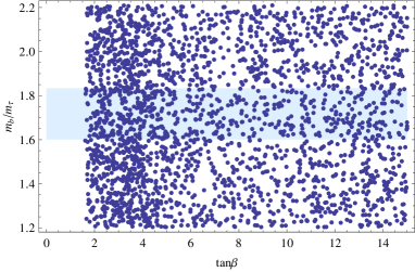
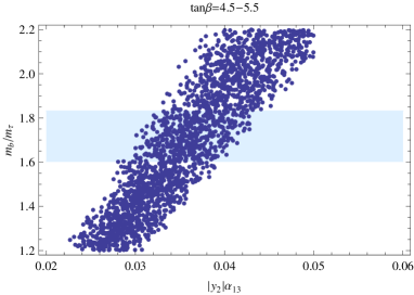
Figure 1: The mass ratio of bottom to tau in the electroweak scale is shown versus (a) $\tan\beta$, and (b) $|y_{2}|a_{13}$ at the GUT scale. The shaded region describes the experimentally arrowed region. All other parameters such as the top mass and neutrino masses are chosen to be consistent with experiments.

Now we can estimate values of $a_{i}$ by using Eq. (26). Putting typical values of quark masses at GUT scale [122], $M=10^{12}~{}\ \text{GeV}$, $\lambda=0.1$, and $\tan\beta=5$ ($v_{d}\simeq 34~{}\text{GeV}$, $v_{u}\simeq 170~{}\text{GeV}$), we have

$$a_{1}\sim 3\times 10^{-2},\quad a_{4}\sim 10^{-2},\quad a_{5}\sim 10^{-2},\qquad a_{9}\sim 5\times 10^{-3},\quad a_{13}\sim 3\times 10^{-2},$$ (57)

where all Yukawa couplings are assumed to be one. If we use smaller Yukawa couplings than $1$, these values of $a_{i}$ are changed in a factor. Therefore, the magnitudes of all $a_{i}$ are supposed to be order $10^{-2}$.

5 LFV and EDM in SUSY flavor

We discuss SUSY flavor phenomena for the lepton sector in the $S_{4}$ model. Mass insertion parameters, $\delta_{\ell}^{LL}$, $\delta_{\ell}^{LR}$, $\delta_{\ell}^{RL}$ and $\delta_{e}^{RR}$ are defined by

$$m_{\tilde{\ell}}^{2}\begin{pmatrix}\delta_{\ell}^{LL}&\delta_{\ell}^{LR}\\ \delta_{\ell}^{RL}&\delta_{e}^{RR}\\ \end{pmatrix}=\begin{pmatrix}m_{\tilde{L}}^{2}&m_{LR}^{2}\\ m_{RL}^{2}&m_{\tilde{R}}^{2}\\ \end{pmatrix}-\text{diag}(m_{\tilde{\ell}}^{2})\ ,$$ (58)

where $m_{\tilde{\ell}}$ is an average slepton mass. In the SCKM basis, they are estimated as

$$\delta_{\ell}^{LL}=\begin{pmatrix}\mathcal{O}(\tilde{a}^{2})&\mathcal{O}(\tilde{a}^{2})&\mathcal{O}(\tilde{a}^{2})\\ \mathcal{O}(\tilde{a}^{2})&\mathcal{O}(\tilde{a}^{2})&\mathcal{O}(\tilde{a}^{2})\\ \mathcal{O}(\tilde{a}^{2})&\mathcal{O}(\tilde{a}^{2})&\mathcal{O}(\tilde{a}^{2})\end{pmatrix},\quad\delta_{e}^{RR}=\begin{pmatrix}\mathcal{O}(\tilde{a}^{2})&\mathcal{O}(\tilde{a}^{2})&\mathcal{O}(a_{1})\\ \mathcal{O}(\tilde{a}^{2})&\mathcal{O}(\tilde{a}^{2})&\mathcal{O}(a_{1})\\ \mathcal{O}(a_{1})&\mathcal{O}(a_{1})&\mathcal{O}(\tilde{a}^{2})\end{pmatrix},$$

$$\delta_{\ell}^{LR}=\frac{1}{m_{\tilde{\ell}}}\begin{pmatrix}\mathcal{O}(\tilde{a}^{2}(1+\frac{\mu\tan\beta}{m_{\tilde{\ell}}})v_{d})&\mathcal{O}(\tilde{a}^{2}v_{d})&\mathcal{O}(\tilde{a}^{2}v_{d})\\ \mathcal{O}(\tilde{a}^{2}v_{d})&\mathcal{O}(m_{\mu}(1+\frac{\mu\tan\beta}{m_{\tilde{\ell}}}))&\mathcal{O}(\tilde{a}^{2}v_{d})\\ \mathcal{O}(\tilde{a}^{2}v_{d})&\mathcal{O}(\tilde{a}^{2}v_{d})&\mathcal{O}(m_{\tau}(1+\frac{\mu\tan\beta}{m_{\tilde{\ell}}}))\end{pmatrix}.$$

With these parameters, we calculate $\ell_{i}\rightarrow\ell_{j}\gamma$ ratios and EDM’s of leptons.

In general, when there are right-handed neutrinos which couple to the left-handed neutrinos via Yukawa coupling, the effects from RG running can also induce off-diagonal elements in the slepton mass matrix. We have already estimated this effect in the previous work [108] as

$$(\delta_{\ell}^{LL})_{12}=\frac{6m_{0}^{2}}{16\pi^{2}m_{\text{SUSY}}^{2}}(Y_{D}^{\dagger}Y_{D})_{12}\ln\frac{\Lambda}{M}\simeq\frac{3}{8\pi^{2}}{y_{2}^{D}}^{2}a_{5}^{2}\ln\frac{\Lambda}{M}\simeq 6\times 10^{-5}\ ,$$ (60)

where we put $m_{0}=m_{\text{SUSY}}$, $a_{5}=10^{-2}$, $\Lambda=10^{16}$ GeV, $M=10^{12}$ GeV. Since the key ingredient $(Y_{D}^{\dagger}Y_{D})_{12}$ is rather small such as $(Y_{D}^{\dagger}Y_{D})_{12}={y_{2}^{D}}^{2}a_{5}^{2}$, the branching ratio is suppressed. It is concluded that the contribution on $\mu\rightarrow e\gamma$ from the neutrino sector is much smaller than the experimental bound $(\delta_{\ell}^{LL})^{\rm exp}_{12}\leq{\cal O}(10^{-3})$ [114]. Therefore, we neglect the effect of the Dirac neutrinos in the following calculations.

5.1 $\mu\to e\gamma$, $\tau\to e\gamma$ and $\tau\to\mu\gamma$

In the framework of SUSY, LFV effects originate from misalignment between fermion and sfermion mass eigenstates. Once non-vanishing off diagonal elements of the slepton mass matrices are generated in the super-CKM basis, LFV rare decays like $\ell_{i}\to\ell_{j}\gamma$ are naturally induced by one-loop diagrams with the exchange of gauginos and sleptons. The present bounds on these processes are summarized in Table 3 [123].

Process	BR($\mu\to e\,\gamma$)	BR($\tau\to e\,\gamma$)	BR($\tau\to\mu\,\gamma$)
Experimental limit	$1.2~{}\times~{}10^{-11}$	$1.1~{}\times~{}10^{-7}$	$6.8~{}\times~{}10^{-8}$

Table 3: Present limits on the lepton flavor violation for each process [123].

The decay $\ell_{i}\to\ell_{j}\gamma$ is described by the dipole operator and the corresponding amplitude reads [114, 120, 124, 125]

$$T=m_{\ell_{i}}\epsilon^{\lambda}\overline{u}_{j}(p-q)[iq^{\nu}\sigma_{\lambda\nu}(A_{L}P_{L}+A_{R}P_{R})]u_{i}(p)\,,$$ (61)

where $p$ and $q$ are momenta of the initial lepton $\ell_{i}$ and of the photon, respectively, and $A_{L,R}$ are the two possible amplitudes in this process. The branching ratio of $\ell_{i}\rightarrow\ell_{j}\gamma$ can be written as follows:

$$\frac{{\rm BR}(\ell_{i}\rightarrow\ell_{j}\gamma)}{{\rm BR}(\ell_{i}\rightarrow\ell_{j}\nu_{i}\bar{\nu_{j}})}=\frac{48\pi^{3}\alpha}{G_{F}^{2}}(|A_{L}^{ij}|^{2}+|A_{R}^{ij}|^{2})\,.$$

In the mass insertion approximation, it is found that [115]

$$A^{ij}_{L} \simeq \frac{\alpha_{2}}{4\pi}\frac{\left(\delta^{LL}_{\ell}\right)_{ij}}{m_{\tilde{\ell}}^{2}}\tan{\beta}~{}\bigg{[}\frac{\mu M_{2}}{(M_{2}^{2}-\mu^{2})}\bigg{(}f_{2n}(x_{2},x_{\mu})+f_{2c}(x_{2},x_{\mu})\bigg{)}$$

$$+\tan^{2}\theta_{W}\,\mu M_{1}\bigg{(}\frac{f_{3n}(x_{1})}{m_{\tilde{\ell}}^{2}}+\frac{f_{2n}(x_{1},x_{\mu})}{(\mu^{2}-M_{1}^{2})}\bigg{)}\bigg{]}+\frac{\alpha_{1}}{4\pi}~{}\frac{\left(\delta^{RL}_{\ell}\right)_{ij}}{m_{\tilde{\ell}}^{2}}~{}\left(\frac{M_{1}}{m_{\ell_{i}}}\right)~{}2~{}f_{2n}(x_{1})~{},$$

$$A^{ij}_{R} \simeq \frac{\alpha_{1}}{4\pi}\left[\frac{\left(\delta^{RR}_{e}\right)_{ij}}{m_{\tilde{\ell}}^{2}}\mu M_{1}\tan{\beta}\left(\frac{f_{3n}(x_{1})}{m_{\tilde{\ell}}^{2}}-\frac{2f_{2n}(x_{1},x_{\mu})}{(\mu^{2}-M_{1}^{2})}\right)+2\frac{\left(\delta^{LR}_{e}\right)_{ij}}{m_{\tilde{\ell}}^{2}}~{}\left(\frac{M_{1}}{m_{\ell_{i}}}\right)~{}f_{2n}(x_{1})\right]~{},$$

where $\theta_{W}$ is the weak mixing angle, $x_{1,2}=M_{1,2}^{2}/m_{\tilde{\ell}}^{2}$, $x_{\mu}=\mu^{2}/m_{\tilde{\ell}}^{2}$ and $f_{i(c,n)}(x,y)=f_{i(c,n)}(x)-f_{i(c,n)}(y)$. The loop functions $f_{i}$’s are given explicitly as follows:

$$\begin{split}f_{2n}(x)&=\frac{-5x^{2}+4x+1+2x(x+2)\log x}{4(1-x)^{4}}~{},\\ f_{3n}(x)&=\frac{1+9x-9x^{2}-x^{3}+6x(x+1)\log x}{3(1-x)^{5}}~{},\\ f_{2c}(x)&=\frac{-x^{2}-4x+5+2(2x+1)\log x}{2(1-x)^{4}}~{}.\end{split}$$ (63)

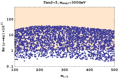
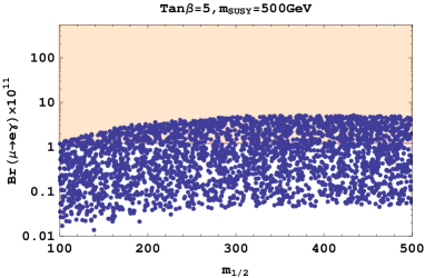
Figure 2: Branching ratio of $\mu\rightarrow e\gamma$ versus the gaugino mass parameter $m_{1/2}$ for (a) $\tan\beta=5$, $m_{\text{SUSY}}=300$GeV, and (b) $\tan\beta=5$, $m_{\text{SUSY}}=500$GeV. Shaded regions show exclusion from current experiments, i.e. Br$(\mu\rightarrow e\gamma)>1.2\times 10^{-11}$.

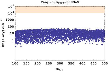
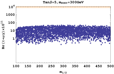
Figure 3: Scattering plots for the branching ratios of $\tau\rightarrow e\gamma$ and $\tau\rightarrow\mu\gamma$ versus gaugino mass $m_{1/2}$. Both are calculated with $\tan\beta=5$ and $m_{\text{SUSY}}=300$GeV. Experimental limits for each processes are $1.1\times 10^{-7}$ and $6.8\times 10^{-8}$, respectively.

In numerical calculations of the $\mu\rightarrow e\gamma$ ratio, we take $\tan\beta=5$, $m_{\text{GUT}}=2\times 10^{16}$GeV, and the SUSY mass scale, $m_{\text{SUSY}}$, as $300$GeV or $500$GeV. We see the dependence of $m_{1/2}$ up to $500$GeV. Gaugino and slepton masses at the electroweak scale can be calculated by $m_{1/2}$ and $m_{\text{SUSY}}$ as in Eqs. (54) and (4). Similarly, $\mu$ parameter is also calculable by putting $\tan\beta$, $m_{1/2}$, and $m_{\text{SUSY}}$, see Eq. (56). We vary absolute values of Yukawa couplings from $0.1$ to $1$ in the calculation. Then, we obtain the numerical result of the branching ratio which is illustrated in Figures 2 (a) and (b). In the branching ratio of Eq. (LABEL:form), there are terms which proportional to the $\mu$-parameter, which increases as the gaugino mass $m_{1/2}$ increases as seen in Eq. (56). Therefore, our predicted branching ratio does not necessarily decrease as $m_{1/2}$ increases.

The predicted region of the ratio with $m_{\text{SUSY}}=300$GeV, $500$GeV lies within the region of expected sensitivity at the MEG experiment [126], concretely, $\mathcal{O}(10^{-13})$–$\mathcal{O}(10^{-14})$. When $m_{\text{SUSY}}=300$GeV, the branching ratio cannot be smaller than $10^{-12}$. Increasing $m_{\text{SUSY}}$ to 500GeV, the lowest value of the ratio is about $10^{-13}$. Thus we expect the observation of the $\mu\rightarrow e\gamma$ process at the MEG experiment [126].

In the same method, we also calculated the branching ratios of $\tau\rightarrow e\gamma$ and $\tau\rightarrow\mu\gamma$ as shown in Figures 3 (a) and (b). All of $\ell_{i}\rightarrow\ell_{j}\gamma$ ratios have the same order due to structures of the slepton mass matrices. Predicted ratios of $\tau\rightarrow e\gamma$ and $\tau\rightarrow\mu\gamma$ are much below the current experimental bounds. Future experiments such as SuperB cannot reach the expected ratios in our flavor model.

5.2 Electric dipole moment

The mass insertion parameters also contribute to the electron EDM through one-loop exchange of binos/sleptons. The corresponding EDM is given as [112, 113, 115]

$$\frac{d_{e}}{e}\!\!=\!\!-\frac{\alpha_{1}}{4\pi}\frac{M_{1}}{m^{2}_{\tilde{\ell}}}\!\!\! \bigg{\{} \!\!\!{\rm Im}[(\delta^{LR}_{\ell})_{1k}(\delta^{RR}_{e})_{k1}+(\delta^{LL}_{\ell})_{1k}(\delta^{LR}_{\ell})_{k1}]\,f_{3n}(x_{1})+{\rm Im}[(\delta^{LL}_{\ell})_{1k}(\delta^{LR}_{\ell})_{kl}(\delta^{RR}_{e})_{l1}$$ (64)

$$+ (\delta^{LR}_{\ell})_{1k}(\delta^{RR}_{e})_{kl}(\delta^{RR}_{e})_{l1}+(\delta^{LL}_{\ell})_{1k}(\delta^{LL}_{\ell})_{kl}(\delta^{LR}_{\ell})_{l1}]\,f_{4n}(x_{1})\bigg{\}}\,,$$

where $k,l=2,3$, $(\delta^{LR}_{\ell})_{33}=-m_{\tau}(A_{\tau}+\mu\tan\beta)/m^{2}_{\tilde{\ell}}$, and the loop function $f_{4n}$ is given as

$$\begin{split}f_{4n}(x)&=\frac{-3-44x+36x^{2}+12x^{3}-x^{4}-12x(3x+2)\log x}{6(1-x)^{6}}\,.\end{split}$$ (65)

Since components $(i,3)$ and $(3,i)$ of $\delta_{e}^{RR}$ are much larger compared to others, dominant terms are given as

$$\frac{d_{e}}{e}\approx-\frac{\alpha_{1}}{4\pi}\frac{M_{1}}{m^{2}_{\tilde{\ell}}} \bigg{\{} \mathcal{O}(\frac{m_{e}}{m_{\tilde{\ell}}}a_{1})\,f_{3n}(x_{1})+\mathcal{O}(\frac{m_{\tau}}{m_{\tilde{\ell}}}(1+\frac{\mu\tan\beta}{m_{\tilde{\ell}}})a_{1}\tilde{a}^{2})\,f_{4n}(x_{1})\bigg{\}}.$$ (66)

In the same parameter regions for the calculation of $\ell_{i}\rightarrow\ell_{j}\gamma$ ratios, we numerically estimate EDM of leptons. We present the result of $|d_{e}|$ in Figure 4 (a), in which $\tan\beta=5$, $m_{\text{SUSY}}=300$GeV and $m_{1/2}=100-500$GeV. Since phases of Yukawa coupling constants are important in this estimate, we randomly choose $0$ to $2\pi$ for phases of all Yukawa couplings. The current experimental bound is $1.6\times 10^{-27}e\text{cm}$ [127], which is denoted by shaded region. Without tuning phase parameters our prediction is below the present experimental bound. We expect the observation of the electron EDM in the future experiment, in which the experimental sensitivity will be improved as $10^{-31}e\text{cm}$ [128].

In Figure 5, we show our predicted region on $|d_{e}|$ and Br$(\mu\rightarrow e\gamma)$ plane for the case $m_{\text{SUSY}}=300$GeV and $m_{1/2}=100$–$300$GeV. As one can see from Figure 5, our predicted region of the electron EDM is not so restricted even if the branching ratio of $\mu\rightarrow e\gamma$ is fixed. For example, when $\mu\rightarrow e\gamma$ decay will be observed just below the present experimental bound, the predicted electron EDM can be large ${\cal O}(10^{-28})e\text{cm}$ or small ${\cal O}(10^{-31})e\text{cm}$, compared to the current experimental bound.

We have also calculated EDM’s of muon and tau. Since the components $(i,3)$ and $(3,i)$ of $\delta_{e}^{RR}$ also dominate EDM’s, predictions are not so different from $|d_{e}|$. Although there is no exact relations among $|d_{e}|$, $|d_{\mu}|$ and $|d_{\tau}|$ due to different Yukawa couplings, we can say that the magnitudes of them are the same order. Numerically, the results of $|d_{\mu}|$ is shown in Figure 6 (a) and $|d_{\tau}|$ in Figure 6 (b).

In our calculations of LFV and EDM of leptons, we have used SUSY parameters $m_{\rm SUSY}=300,~{}500$GeV and $m_{\rm 1/2}=100-500$GeV. In these parameter regions, we have estimated the SUSY contribution on the anomalous magnetic moment $a_{\mu}=(g-2)_{\mu}/2$, in which the experimental allowed value: $\Delta a_{\mu}=a_{\mu}^{\text{exp}}-a_{\mu}^{\text{SM}}\simeq(3\pm 1)\times 10^{-9}$ [115]. We have checked that the SUSY contribution on the anomalous magnetic moment is within the experimental allowed value in all cases of Figures 2–6.

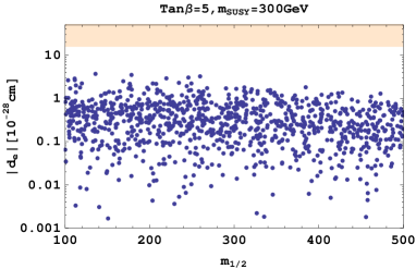
Figure 4: Electric dipole moment of the electron versus gaugino mass. The current experimental bound is $1.6\times 10^{-27}$[$e$cm].

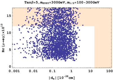
Figure 5: The branching ratio $\mu\rightarrow e\gamma$ versus the electric dipole moment the electron, where $m_{\text{SUSY}}=300$GeV, $m_{1/2}=100-300$GeV and $\tan\beta=5$.

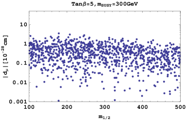
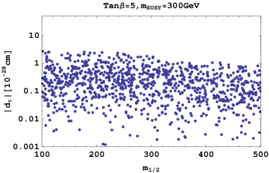
Figure 6: Electric dipole moments of (a) muon and (b) tau, where $m_{\text{SUSY}}=300$GeV, $m_{1/2}=100-500$GeV and $\tan\beta=5$.

6 Summary

There appear many flavor models with the non-Abelian discrete symmetry within the framework of SUSY. The flavor symmetry controls the squark and slepton mass matrices as well as the quark and lepton mass matrices. Therefore, the flavor models could be tested in the squark and slepton sectors. We have discussed slepton mass matrices in the $S_{4}$ flavor model with SUSY $SU(5)$ GUT. By considering the gravity mediation within the framework of supergravity theory, we have estimated the SUSY breaking in the slepton mass matrices, which give the prediction for the $\mu\rightarrow e+\gamma$ decay and the electron EDM.

By taking Yukawa couplings to be in the region of $0.1$ to $1$ without tuning, we have obtained a lower bound for the ratio of $\mu\rightarrow e\gamma$ as $10^{-13}$ if $m_{\text{SUSY}}$ and $m_{1/2}$ are below $500$GeV. This predicted value will be testable at the MEG experiment. The off diagonal terms of slepton mass matrices, which come from the SUSY breaking, also contribute to EDM of leptons. The natural prediction of the electron EDM is around $10^{-29}-10^{-28}e$cm, which can be tested by future experiments. In our calculation, we take $\Lambda$ to be the GUT scale. Our predicted values crucially depend on $a_{i}=\langle\chi_{i}\rangle/\Lambda$, but not $\Lambda$. Since magnitudes of $a_{i}$ are determined by quark and lepton masses, our predictions are not changed even if the $S_{4}$ scale $\Lambda$ is taken to be much larger or smaller than the GUT one.

As shown in this work, the SUSY sector provides us rich fields of investigating flavor models with the non-Abelian discrete symmetry.

Acknowledgement

We owe the $S_{4}$ flavor model to Y. Shimizu. H.I. is supported by Grand-in-Aid for Scientific Research, No.21.5817 from the Japan Society of Promotion of Science. The work of M.T. is supported by the Grant-in-Aid for Science Research, No. 21340055, from the Ministry of Education, Culture, Sports, Science and Technology of Japan.

Appendix A Multiplication rule of $S_{4}$

The $S_{4}$ group has 24 distinct elements and irreducible representations ${\bf 1},~{}{\bf 1}^{\prime},~{}{\bf 2},~{}{\bf 3}$, and ${\bf 3}^{\prime}$. The multiplication rule depends on the basis. One can see its basis dependence in our review [9]. We present the multiplication rule, which is used in this paper:

$$\begin{pmatrix}a_{1}\\ a_{2}\end{pmatrix}_{\bf 2}\otimes\begin{pmatrix}b_{1}\\ b_{2}\end{pmatrix}_{\bf 2} =(a_{1}b_{1}+a_{2}b_{2})_{{\bf 1}}\oplus(-a_{1}b_{2}+a_{2}b_{1})_{{\bf 1}^{\prime}}\oplus\begin{pmatrix}a_{1}b_{2}+a_{2}b_{1}\\ a_{1}b_{1}-a_{2}b_{2}\end{pmatrix}_{{\bf 2}\ ,}$$ (67)

$$\begin{pmatrix}a_{1}\\ a_{2}\end{pmatrix}_{\bf 2}\otimes\begin{pmatrix}b_{1}\\ b_{2}\\ b_{3}\end{pmatrix}_{{\bf 3}} =\begin{pmatrix}a_{2}b_{1}\\ -\frac{1}{2}(\sqrt{3}a_{1}b_{2}+a_{2}b_{2})\\ \frac{1}{2}(\sqrt{3}a_{1}b_{3}-a_{2}b_{3})\end{pmatrix}_{{\bf 3}}\oplus\begin{pmatrix}a_{1}b_{1}\\ \frac{1}{2}(\sqrt{3}a_{2}b_{2}-a_{1}b_{2})\\ -\frac{1}{2}(\sqrt{3}a_{2}b_{3}+a_{1}b_{3})\end{pmatrix}_{{\bf 3}^{\prime}\ ,}$$ (68)

$$\begin{pmatrix}a_{1}\\ a_{2}\end{pmatrix}_{\bf 2}\otimes\begin{pmatrix}b_{1}\\ b_{2}\\ b_{3}\end{pmatrix}_{{\bf 3}^{\prime}} =\begin{pmatrix}a_{1}b_{1}\\ \frac{1}{2}(\sqrt{3}a_{2}b_{2}-a_{1}b_{2})\\ -\frac{1}{2}(\sqrt{3}a_{2}b_{3}+a_{1}b_{3})\end{pmatrix}_{{\bf 3}}\oplus\begin{pmatrix}a_{2}b_{1}\\ -\frac{1}{2}(\sqrt{3}a_{1}b_{2}+a_{2}b_{2})\\ \frac{1}{2}(\sqrt{3}a_{1}b_{3}-a_{2}b_{3})\end{pmatrix}_{{\bf 3}^{\prime}\ ,}$$ (69)

$$\begin{pmatrix}a_{1}\\ a_{2}\\ a_{3}\end{pmatrix}_{{\bf 3}}\otimes\begin{pmatrix}b_{1}\\ b_{2}\\ b_{3}\end{pmatrix}_{{\bf 3}} =(a_{1}b_{1}+a_{2}b_{2}+a_{3}b_{3})_{{\bf 1}}\oplus\begin{pmatrix}\frac{1}{\sqrt{2}}(a_{2}b_{2}-a_{3}b_{3})\\ \frac{1}{\sqrt{6}}(-2a_{1}b_{1}+a_{2}b_{2}+a_{3}b_{3})\end{pmatrix}_{\bf 2}$$

$$\ \oplus\begin{pmatrix}a_{2}b_{3}+a_{3}b_{2}\\ a_{1}b_{3}+a_{3}b_{1}\\ a_{1}b_{2}+a_{2}b_{1}\end{pmatrix}_{{\bf 3}}\oplus\begin{pmatrix}a_{3}b_{2}-a_{2}b_{3}\\ a_{1}b_{3}-a_{3}b_{1}\\ a_{2}b_{1}-a_{1}b_{2}\end{pmatrix}_{{\bf 3}^{\prime}\ ,}$$ (70)

$$\begin{pmatrix}a_{1}\\ a_{2}\\ a_{3}\end{pmatrix}_{{\bf 3}^{\prime}}\otimes\begin{pmatrix}b_{1}\\ b_{2}\\ b_{3}\end{pmatrix}_{{\bf 3}^{\prime}} =(a_{1}b_{1}+a_{2}b_{2}+a_{3}b_{3})_{{\bf 1}}\oplus\begin{pmatrix}\frac{1}{\sqrt{2}}(a_{2}b_{2}-a_{3}b_{3})\\ \frac{1}{\sqrt{6}}(-2a_{1}b_{1}+a_{2}b_{2}+a_{3}b_{3})\end{pmatrix}_{\bf 2}$$

$$\ \oplus\begin{pmatrix}a_{2}b_{3}+a_{3}b_{2}\\ a_{1}b_{3}+a_{3}b_{1}\\ a_{1}b_{2}+a_{2}b_{1}\end{pmatrix}_{{\bf 3}}\oplus\begin{pmatrix}a_{3}b_{2}-a_{2}b_{3}\\ a_{1}b_{3}-a_{3}b_{1}\\ a_{2}b_{1}-a_{1}b_{2}\end{pmatrix}_{{\bf 3}^{\prime}\ ,}$$ (71)

$$\begin{pmatrix}a_{1}\\ a_{2}\\ a_{3}\end{pmatrix}_{{\bf 3}}\otimes\begin{pmatrix}b_{1}\\ b_{2}\\ b_{3}\end{pmatrix}_{{\bf 3}^{\prime}} =(a_{1}b_{1}+a_{2}b_{2}+a_{3}b_{3})_{{\bf 1}^{\prime}}\oplus\begin{pmatrix}\frac{1}{\sqrt{6}}(2a_{1}b_{1}-a_{2}b_{2}-a_{3}b_{3})\\ \frac{1}{\sqrt{2}}(a_{2}b_{2}-a_{3}b_{3})\end{pmatrix}_{\bf 2}$$

$$\ \oplus\begin{pmatrix}a_{3}b_{2}-a_{2}b_{3}\\ a_{1}b_{3}-a_{3}b_{1}\\ a_{2}b_{1}-a_{1}b_{2}\end{pmatrix}_{{\bf 3}}\oplus\begin{pmatrix}a_{2}b_{3}+a_{3}b_{2}\\ a_{1}b_{3}+a_{3}b_{1}\\ a_{1}b_{2}+a_{2}b_{1}\end{pmatrix}_{{\bf 3}^{\prime}\ .}$$ (72)

More details are shown in the review [9].