A robust two-gene oscillator at the core of Ostreococcus tauri circadian clock

Abstract

The microscopic green alga Ostreococcus tauri is rapidly emerging as a promising model organism in the green lineage. In particular, recent results by Corellou et al. [Plant Cell 21, 3436 (2009)] and Thommen et al. [PLoS Comput. Biol. 6, e1000990 (2010)] strongly suggest that its circadian clock is a simplified version of Arabidopsis thaliana clock, and that it is architectured so as to be robust to natural daylight fluctuations. In this work, we analyze time series data from luminescent reporters for the two central clock genes TOC1 and CCA1 and correlate them with microarray data previously analyzed. Our mathematical analysis strongly supports both the existence of a simple two-gene oscillator at the core of Ostreococcus tauri clock and the fact that its dynamics is not affected by light in normal entrainment conditions, a signature of its robustness.

In order to anticipate periodic environmental changes induced by Earth rotation, many organisms have evolved a circadian clock, a genetic oscillator which generates biochemical rhythms with a period around 24 hours. Exact synchronization with the day/night cycle requires that one or more clock components sense daylight (for example, a protein degrades faster in the light). However, daylight intensity can highly fluctuate from day to day, or during the day, due to environmental factors such as sky cover. The question then arises as to how circadian clocks can keep time without being continously reset by the signal that should entrain them? A mathematical analysis of Ostreococcus tauri clock, whose molecular basis has been identified recently Corellou et al. (2009), has unveiled a simple and elegant mechanism which exploits the dynamical properties of the core clock oscillator to make it robust to daylight fluctuations Thommen et al. (2010). When the clock is on time, coupling to light is activated precisely when the oscillator does not respond to external perturbations, making it blind to light and its fluctuations. If the clock has drifted and needs resetting, however, light affects the oscillator in a different part of its cycle, where it reacts so as to recover the entrainment phase. In this work, we provide strong evidence for the presence of a robust two-gene oscillator at the core of Ostreococcus clock by showing that a minimal light-independent model can reproduce very accurately microarray data and luminescent reporter data recorded in different experiments.

I Introduction

Biochemical oscillations are widespread biological phenomena involved in many important cellular processes such as signaling, development, motility or metabolism Goldbeter (1996); Hasty, Hoffmann, and Golden (2010). Understanding how such a simple dynamical pattern has been implemented repeatedly to support a great diversity of biological functions is appealing for scientists seeking to uncover unifying principles Winfree (2001). By identifying the molecular machinery behind cellular rhythms, molecular biology has first laid the groundwork for the development of strategies toward their comprehensive understanding Young (1993). In a second stage, how a collective dynamics can emerge in networks of interacting molecular actors and how it can be harnessed robustly has been under focus. Besides the design of synthetic genetic circuits with specific oscillatory abilities Elowitz and Leibler (2000); Stricker et al. (2008), a common strategy to gain insight into this question has been to construct quantitative dynamical models constrained by experiments Goldbeter (1996); Hartwell et al. (1999); Tiana et al. (2007); Mengel et al. (2010). Indeed, the nonlinear dynamical behaviors that underlie oscillations can only be fully captured through a mathematical description.

However, the ever-growing amount of experimental data obtained with genetic transformations and real-time monitoring presents extraordinary challenges to modelers. How to design relevant mathematical models that not only reproduce the data but give insight into the architecture of a biological system, and avoid pitfalls such as overfitting which can ascribe biological meaning to experimental artifacts? As we hope to illustrate here, it is important to combine careful data analysis and minimal modeling, and to check the consistence of the different data sets at all stages of model building.

Circadian clocks are systems of choice for quantitative studies of the function and design of biochemical oscillators Rand et al. (2004). They operate in many species to keep track of the most regular environmental constraint, the alternation of daylight and darkness caused by Earth rotation, so as to finely control the cellular physiology accordingly Pittendrigh (1960). This basic function is vital in many organisms such as plants, which need to timely coordinate their photosynthesis, and thus their growth and division, to daily changes in light intensity Dodd et al. (2005); Moulager et al. (2007); Monnier et al. (2010). However, a precise entrainment of circadian rhythms to the diurnal cycle is potentially challenged by many sources of variability including molecular fluctuations Gonze, Halloy, and Goldbeter (2002); Barkai and Leibler (2000) and temperature variations Pittendrigh (1954); Rensing and Ruoff (2002), but also fluctuations of daylight intensity from day to day or during the day, due to environmental factors such as sky cover Comas et al. (2008); Beersma, Daan, and Hut (1999); Troein et al. (2009); Thommen et al. (2010). To account for the remarkable ability of circadian oscillators to run autonomously and to be precisely and robustly entrained, experimental efforts aimed at unraveling their complex architecture Dunlap (1999); Young and Kay (2001); Panda, Hogenesch, and Kay (2002) have motivated studies trying to adjust mathematical models to experimental data Forger and Peskin (2003); Forger et al. (2003); Locke et al. (2005, 2006); Zeilinger et al. (2006); Salazar et al. (2009); Thommen et al. (2010); François (2005), an approach that is increasingly necessary as models become more complex, featuring generally several feedback loops.

In this paper, we use such a quantitative modeling approach to investigate the dynamics of the circadian rhythms of the smallest free-living eukaryote known to date, Ostreococcus tauri. This microscopic green alga displays a very simple cellular organization and a small and compact genome Courties et al. (1994); Chretiennot-Dinet et al. (1995); E. Derelle et al. (2006). Very recently, the molecular basis of its circadian clock has been extensively characterized by Corellou et al., who carried out an extensive work of genetic transformation, leading to transcriptional and translational fusion lines allowing one to monitor transcriptional activity and protein dynamics in living cells Corellou et al. (2009); Djouani-Tahri et al. (2010). Their results point to a core archictecture comprising two genes, similar to Arabidopsis central clock genes TOC1 and CCA1 Alabadi et al. (2001). These two genes display rhythmic expression both under light/dark alternation and in constant light conditions. Thus, the unicellular green alga Ostreococcus tauri has emerged as a promising organism model to study the circadian rhythm in single photosynthetic eukaryotic cell combining experimental and modeling approaches.

The goal of this modeling study is to check carefully whether experimental data obtained through various channels support the hypothesis that the circadian clock of Ostreococcus Tauri contains a simple two-gene transcriptional loop serving as a core oscillator Corellou et al. (2009); Thommen et al. (2010), and that the dynamics of this oscillator is not affected by light in normal entrainment conditions Thommen et al. (2010). An important point of the present work is the simultaneous adjustment of microarray data and luminescent reporter data recorded in two different experiments Moulager et al. (2007); Corellou et al. (2009) under different conditions. While this may not be sensible for a general system whose parameters will typically change with experimental conditions, it is expected here that the core clock oscillator is robust to environmental changes. As advocated by Thommen et al. Thommen et al. (2010), it should thus deliver similar signals in different experiments carried out with the same photoperiod. Therefore, being able to reproduce with the same model signals recorded with different techniques in different experiments provides strong evidence that the core Ostreococcus clock oscillator is indeed robust.

Before adjusting a minimal model to experimental data, a careful data analysis of both microarray and luminescence time series has been performed. It allowed us to detect and remove an experimental artifact that would otherwise have prevented an optimal adjustment and thus would have falsely called for a more complex model. The combined use of microarray data and luminescence reporter data provided a unique opportunity to calibrate the latter with respect to the former, given that very little is known on luciferase dynamics in Ostreococcus. This is all the more important as an extensive collection of experimental data has been acquired with these reporters and will form the basis of future quantitative studies of Ostreococcus clock.

We not only found that a simple two-gene transcriptional feedback loop model reproduces perfectly the CCA1 and TOC1 transcript and protein profiles obtained from data analysis, but that it does so with no model parameter depending on light intensity whereas the data have been recorded under light/dark alternation. This confirms our previous observation based only on microarray data of limited time resolution Thommen et al. (2010). As we have proposed previously, this counterintuitive finding indicates that the coupling to light does not influence the oscillator in normal entrainment conditions, shielding it from daylight fluctuations Thommen et al. (2010). Besides confirming the two-gene loop hypothesis and the oscillator robustness, this work also identifies unambiguously the mechanistic origin of oscillation in the transcriptional negative feedback loop involving CCA1 and TOC1, delayed by the saturated degradation of CCA1 mRNA and TOC1 protein.

II Data Analysis

In this section, we first present the experimental data and explain how we determine mRNA and protein concentrations from them. We then discuss the simplest model of the TOC1–CCA1 negative feedback loop, which consists of four differential equations describing the time evolution of the TOC1 and CCA1 mRNA and protein concentrations. To match the numerical time profiles generated by this model, we need to reconstruct target profiles from the experimental data. RNA profiles will be interpolated from microarray data whereas protein profiles will be extracted from luminescence time series in the form of a Fourier series describing the dynamics at long time scales. Both types of profile will be characterized by their times of passage at $20\%$ and $80\%$ of the oscillation amplitude, which provide a uniform characterization of the two types of data considered here. Model adjustment will be carried out by minimizing discrepancies between the experimental and numerical passage times.

II.1 Experimental data

The microarray data used here come from the study in Ref. Moulager et al. (2007). They were recorded at three-hour time intervals under 12:12 light/dark alternation. The mRNA time profiles that will serve as targets for model adjustment are the same as in our previous study Thommen et al. (2010), where we showed that they could be accurately approached by solutions of a simple set of differential equations, an indication of the high quality of these data. The fact that microarray data reflect mRNA level without ambiguity was also checked by quantitative RT-PCR.

The luminescent reporter data used here are those presented by Corellou et al. in Corellou et al. (2009) to provide evidence of the central role of the TOC1 and CCA1 genes in Ostreococcus clock. They had been recorded at one-hour intervals under a 12:12 light/dark cycle from two types of transgenic cell lines.

In transcriptional fusion lines pTOC1:luc and pCCA1:luc, the sequence inserted into the genome consists of the promoter of one of the two clock genes fused to the coding sequence of firefly luciferase Corellou et al. (2009), so that TOC1 or CCA1 transcriptional activity drives luciferase expression. Luciferase catalyzes the transformation of the substrate luciferin into oxyluciferin, in which one photon is emitted Gates and DeLuca (1975). The luminescence signal provides information about the quantity of luciferase synthesized and thus on the transcriptional activity of the promoters.

In translational fusion lines TOC1:luc and CCA1:luc, both the coding sequences of one of the clock proteins (TOC1 or CCA1) and of luciferase are fused to the promoter Corellou et al. (2009), so that a fusion protein combining the clock protein with luciferase is synthesized by the additional gene with a trancriptional activity similar to the original clock gene. In this case, the luminescence signal also provides information about the protein dynamics, and in particular on its degradation kinetics. It is usually assumed that luciferase remains complexed and inactive after the reaction and does not recover its activity before being degraded. Thus two limiting cases can be considered depending on whether the luciferase reaction time (defined as the average time from synthesis to photon emission) is much shorter or much longer that the protein lifetime.

In the former case, luciferase reacts immediately after being synthesized. Since only freshly made proteins then contribute to the luminescence signal, the latter is obviously proportional to the protein synthesis rate, hence to cytoplasmic fusion mRNA concentration. If we assume for simplicity that the kinetic constants (synthesis and degradation rates) of the fusion proteins TOC:luc and CCA1:luc and of their mRNA are similar to that of their native counterparts, then the concentrations of the former are proportional to the concentrations of the latter. In this case, the luminescence signal tracks mRNA concentration.

In the opposite case where the probability of photon emission by luciferase is very low, and with the same assumption of identical constants for fusion and native molecular actors, it is easily seen that the luminescence signal is proportional to protein concentration. In this limit, indeed, the photon emission probability is constant throughout protein lifetime, thus luminescence intensity is proportional to the number of TOC1:luc or CCA1:luc fusion proteins, which is in turn proportional to the number of native clock proteins. In this case the luminescence signal can be used as an indicator of protein concentration. In the general case, it should be intermediate between the RNA and protein time courses.

A time lag of at least two hours between the maxima of RNA concentration as indicated by microarray data and the maxima of translational fusion lines can be observed, which indicates that photon emission probability is low and that luciferase lifetime is large compared to other protein lifetimes. This is consistent with recent experiments in which translation was blocked in Ostreococcus cell cultures with emetine dihydrochloride Djouani-Tahri et al. (2010) and time evolution of TOC:luc luminescence was monitored. It was observed that the signal would slowly decay over more than 12 hours, implying that the luciferase reaction time is at least of this order. Thus, we will use in the following translational fusion line signals as indicators of protein concentrations, which allows us to keep our mathematical model as simple as possible.

II.2 Model of the TOC1–CCA1 oscillator used for data adjustment

The minimal model for the TOC1–CCA1 transcriptional feedback loop, where TOC1 activates CCA1 and CCA1 represses TOC1, consists of the following four ordinary differential equations:

$$\dot{M_{T}} = \mu_{T}+\frac{\lambda_{T}}{1+(P_{C}/P_{C0})^{n_{C}}}-\delta_{M_{T}}\frac{K_{M_{T}}M_{T}}{K_{M_{T}}+M_{T}}$$ (1a)

$$\dot{P_{T}} = \beta_{T}M_{T}-\delta_{P_{T}}\frac{K_{P_{T}}P_{T}}{K_{P_{T}}+P_{T}}$$ (1b)

$$\dot{M_{C}} = \mu_{C}+\frac{\lambda_{C}(P_{T}/P_{T0})^{n_{T}}}{1+(P_{T}/P_{T0})^{n_{T}}}-\delta_{M_{C}}\frac{K_{M_{C}}M_{C}}{K_{M_{C}}+M_{C}}$$ (1c)

$$\dot{P_{C}} = \beta_{C}M_{C}-\delta_{P_{C}}\frac{K_{P_{C}}P_{C}}{K_{P_{C}}+P_{C}}$$ (1d)

Eqs. (1) describe the time evolution of mRNA concentrations $M_{C}$ and $M_{T}$ and protein concentrations $P_{C}$ and $P_{T}$ for the CCA1 and TOC1 genes, respectively, as they result from mRNA synthesis regulated by the other protein, translation and enzymatic degradation. TOC1 transcription rate varies between $\mu_{T}$ at infinite CCA1 concentration and $\mu_{T}+\lambda_{T}$ at zero CCA1 concentration according to the usual gene regulation function with threshold $P_{C0}$ and cooperativity $n_{C}$. Similarly, CCA1 transcription rate is $\mu_{C}$ (resp., $\mu_{C}+\lambda_{C}$) at zero (resp., infinite) TOC1 concentration, with threshold $P_{T0}$ and cooperativity $n_{T}$. TOC1 and CCA1 translation rates are $\beta_{T}$ and $\beta_{C}$, respectively. For each species $X$, the Michaelis-Menten degradation term is written so that $\delta_{X}$ is the low-concentration degradation rate and $K_{X}$ is the saturation threshold.

A more detailed model would take into account compartmentalization, with each actor having separate nuclear and cytoplasmic concentrations, as well as the fact that the luminescence signal is linked to a third gene artificially inserted in the genome, with the kinetic constants of its mRNA and protein possibly different from those of its native counterpart. With this model, it is the profile predicted for the total fusion protein concentration that would be adjusted to the experimental time series rather than the native protein profile. However, the important point is that such a biochemically detailed model taking into account all native and inserted molecular actors reduces to Eqs. (1) in the limiting case where fusion proteins and mRNA have the same kinetic constants as the native molecules (e.g., TOC1:luc and TOC1 degradation rates are equal), luciferase reaction time is large and nucleocytoplasmic transport is fast. When the minimal model already adjusts the data with excellent accuracy, as will be the case here, there is no point in using the sophisticated model, which can only fit the data better. In fact, its higher flexibility could lead to overfit the data and ascribe incorrectly biological meaning to experimental artifacts.

As in Thommen et al. (2010), the free-running period (FRP) of the uncoupled oscillator is chosen equal to 24 hours, which was the mean value observed in experiments Corellou et al. (2009). In this case, this oscillator is adjusted to experimental data without modulation since our goal in this work is to show that the average oscillation does not carry any signature of coupling to light. As a control, we will also consider adjustment to oscillators of FRP 23.8 and 25 hours under day conditions. In these two cases, a small modulation of some parameters is required to achieve frequency locking. To keep the FRP fixed during adjustment, we rescale kinetic parameters after each optimization step so that the period of the free-running limit cycle matches the desired value. This subsequently applies to the parameter set which the adjustment converges to.

II.3 Reconstruction of target profiles and determination of passage times

Experimental RNA target profiles were estimated from the same microarray data points as used in Thommen et al. (2010). Due to the high quality of data, noise reduction was not required. However, the relatively low temporal resolution (one sample every three hours) made it difficult to estimate accurately passage times and positions of expression peaks. Thus the profiles were obtained by interpolating between data points. Time series in the logarithm of RNA concentration showed a very smooth behavior and were well approximated by simple cubic splines (Fig. 1). These interpolating curves were thus considered to provide an optimal approximation to the variations of the logarithm of mRNA concentration, and mRNA linear target curves were generated by exponentiation of the interpolating curves.

That the largest data point is less than half of the maximum of the reconstructed TOC1 mRNA profile should not be surprising. In fact, this profile is the most probable one given the data points if we assume sufficient smoothness, or equivalently that the same dynamics acts over the 24-hour cycle. Any other curve would imply fast, transient, processes not linked to the TOC1–CCA1 loop. Since RNA concentration rises from almost zero at ZT6 (Zeitgeber Time 6, i.e., 6 hours after dawn) to almost the maximum level measured at ZT9 and decays from the same level at ZT12 to almost zero at ZT15, it is indeed obvious that the true maximum located between ZT9 and ZT12 must be much higher than the two largest data points. Incorrectly assuming that the largest data point is the profile maximum would in fact bias the analysis.

We checked that interpolating either the CCA1 mRNA concentrations or their logarithms lead to two almost superimposing profile curves, showing that both sequences of values provide the same information. However the profile interpolated directly from TOC1 mRNA concentrations rather than from their logarithms was highly nonphysical, with interpolated concentrations becoming clearly negative on each side of the expression peak. This is a direct consequence of the fact that only two data points are well above the zero level. Implicit in the interpolation procedure is the reconstruction of successive time derivatives of a function from its values at different points. The long sequence of almost zero data points makes the correspondence between function values and time derivatives nearly singular, so that the reconstruction is highly unstable. During the time interval near zero, all time derivatives up to high order appear to be zero, then jump to high values at the beginning and the end of the expression peak. Since the interpolation error is proportional to the maximum value of the fourth time derivate in the interval, the resulting approximation is poor.

The series of logarithms of TOC1 mRNA concentrations does not have this problem and allows optimal reconstruction of the TOC1 mRNA profile. The fact that the logarithm of a time series with long intervals near zero provides more information about the dynamics than the original time series has also been noted in the analysis of chaotic time series Lefranc, Hennequin, and Glorieux (1992); Letellier and Aguirre (2010). Furthermore, it should be noted that many statistical analyses of microarray data use the logarithms of mRNA concentrations because they are more evenly distributed and provide more information.

Compared to a more usual method based on least-square-fitting the data points (as used in Thommen et al. (2010)), this interpolation procedure can only make adjustment more difficult, since it constrains tightly the shape of the profile. However, it is fully consistent with the good agreement found with a low-dimensional ODE set in our previous study Thommen et al. (2010). The passage times were then determined as the times at which the interpolated profile would cross the appropriate level (Fig. 1).

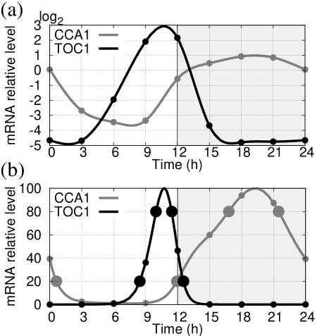
Figure 1: Construction of RNA target profiles as functions of Zeitgeber Time (ZT) describing phases within the dark/light cycle, with time ZT0 corresponds to dawn and time ZT12 to dusk. Interpolating curves going through data points (dots) are represented. (a) Interpolated curves from microarray data using cubic splines. (b) The exponentials of the interpolating curves were computed to obtain a smooth approximation of mRNA profiles. Large dots indicate passages through levels corresponding to 20% and 80% of maximum amplitude and serve as target points for adjustment.

Protein profiles were reconstructed from translational fusion luminescence signals used as indicators of protein concentrations, as discussed above. The reconstruction was more involved than for mRNA because these time series display significant amplitude variations from peak to peak across the experiment, which may be for instance linked to variations in the number of cells contributing to light emission or other experimental factors.

The first 48 recording hours, considered as transient, were discarded and traces were then least-squares fitted by the product $p(t)F(t)$ of a Fourier series $F(t)=\sum_{k=0}^{N}a_{k}\cos(2\pi kt/T+\phi_{k})$, with $T=24$ hours, by a low-order polynomial $p(t)$ accounting for slowly varying experimental conditions (Fig. 2). The order of the polynomial $p(t)$ was generally chosen to be $3$ or $4$, roughly equal to the number of periods in the fitted segment to avoid over-fitting. The Fourier series $F(t)$ represents the average periodic biochemical oscillation associated with circadian oscillations while $p(t)$ models a slowly varying gain (due for example to a variable number of cells contributing to light emission).

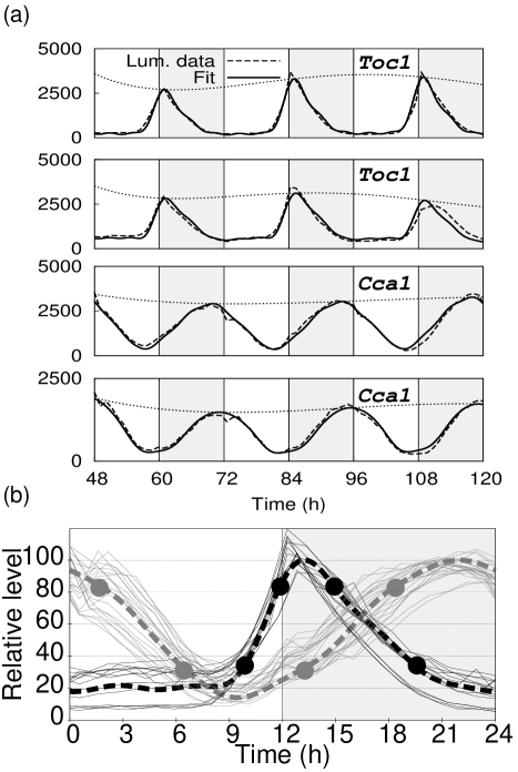
Figure 2: Reconstruction of protein target profiles as functions of Zeitgeber Time (ZT) describing phases within the dark/light cycle, with time ZT0 corresponds to dawn and time ZT12 to dusk. (a) Luminescence time series (dashed lines) for individual wells are fitted by the product of a Fourier series of period 24 hours with 5 harmonics by a slowly varying polynomial function of degree 4 (solid lines). The slowly varying envelope is also shown with a dotted line. From top to bottom, the first (last) two panels correspond to two TOC1:luc (CCA1:luc) translational fusion lines with different insertions in the genome. The different Fourier series are normalized to have the same maximum and are averaged. (b) The average Fourier series (dashed lines, black: TOC1, grey: CCA1) provides a smooth approximation to the cloud of individual line time profiles renormalized using the slowly varying polynomial function and wrapped around 24 hours (thin solid lines). Large dots indicate passages through levels corresponding to 20% and 80% of maximum amplitude and serve as target points for adjustment.

Because we are interested in long lasting mechanisms sustaining the oscillation, the number $N$ of harmonics of the Fourier series was fixed to 5 (an odd number, since the spectrum of the square wave forcing by light only contains odd harmonics). We also tried slightly higher numbers of harmonics, with little difference in the results. Fourier fitting naturally smoothes out acute responses at day/night and night/day transitions that can be seen in the raw signals and which may reflect rapid mechanisms involved in clock resetting. This separation of dynamical processes occurring on a 24-hour time scale on the one hand, and confined to short time intervals on the other hand, must be understood with reference to our previous finding that the average dynamics of the TOC1–CCA1 oscillator is identical to that of a free-running oscillator, with coupling to light and resetting occuring transiently in specific time intervals Thommen et al. (2010). Confirming this key observation with a careful analysis of the luminescence time series is one of the main goals of this paper. It will be reached if we find that the average protein profile does not carry any signature of a coupling to light.

The Fourier series obtained from the fits of all bioluminescence traces (possibly corresponding to different transgenic lines) recorded in the experiment were then averaged, and the average was used as surrogate for the protein temporal profile after suitable normalization. The resulting profile is shown in Fig. 2(b), along with individual luminescence traces from different wells, renormalized using the slowly varying polynomial function $p(t)$. The variability observed is partially due to the fact that a few different transgenic lines, corresponding to different insertions in the genome, were used. The times of passage at $20\%$ and $80\%$ of the amplitude were then determined, as well as the minimal level reached, for subsequent model adjustment.

We also tried fitting each luminescence trace to $p(t)F(t)+b$ where $b$ represents a possible constant bias. Surprisingly, the fit was consistently better when $b$ was equal to the minimum luminescence level. In other words, the Fourier fitting procedure tended to remove the floor level. Because this could indicate the existence of a bias in the luminescence level, we examined more closely the raw data, and found that indeed the zero luminescence level does not correspond to the zero protein level.

In Fig. 3, we show two individual traces monitoring luminescence intensities over time in two wells of the luminometer plate. These two wells contain genetically identical cell cultures monitored simultaneously in the same experiment. Besides an excellent overall reproducibility, the comparison of the two traces reveals the existence of a significant bias. Assuming that identical clocks run in different cells, and that there is a well-defined average number of fusion proteins per cell, the luminescence signals should be proportional to numbers of cells in each well. Therefore, the two signals should be approximately proportional to each other.

Contrary to this, we observe that both for TOC1:luc and CCA1:luc, the maxima of the two signals differ by a large factor, which remains roughly constant over time while minima almost coincide. If the two traces were proportional to each other, the minima should be in the same ratio as the maxima. The only simple explanation for the systematic coincidence of minima is that they correspond to a zero protein level, and that there is the same bias on the two time series. This bias can therefore be removed by substracting the two traces, as is shown in Fig. 3, where the difference curves provide a better estimation of the actual protein profiles than the original traces. Importantly, the CCA1 protein level is predicted to touch zero very shortly near ZT9, while the TOC1 protein level appears to stay near zero for a large interval of time between ZT21 and ZT8 (Fig. 3). Note that this bias is not constant in time but varies slowly so that the different minima correspond to different luminescence levels.

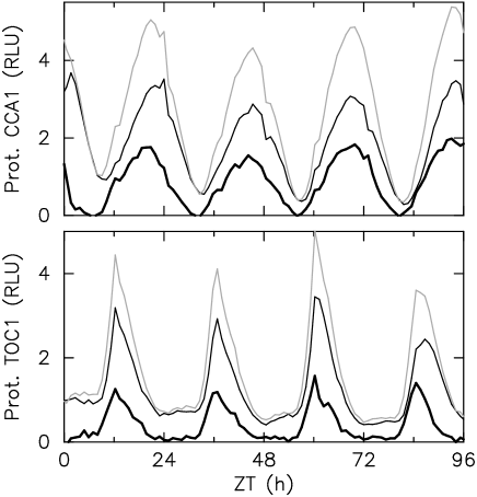
Figure 3: Translational fusion lines data recorded under 12:12 LD alternation. Time zero corresponds to dawn. On top panel (resp., bottom panel) the time evolution of photon count (in relative luminescence units) of CCA1 (resp., TOC1) translational fusion lines are drawn for two biological duplicates monitored at the same time in the same conditions (black and grey thin solid lines). Their difference is plotted as a thick black solid line.

While the existence of an experimental bias in the luminescence level is strongly supported by the observations above, we have currently no explanation for it. In the following, we will therefore adjust two versions of the experimental profiles : (i) the Fourier series $F(t)$ determined directly from fitting $p(t)F(t)$ to the time series, as described above, as if there was no bias, and (ii) the same Fourier series with the floor level removed so that they touch zero, as with the difference curves in Fig. 3. More precisely, the target curves are then $F(t)-F_{0}$ where the $F(t)$ are obtained from fitting $p(t)F(t)$ and $F_{0}=\min_{t}F(t)$. This will allow us to assess the influence of the bias on model fitting. Again, using a more sophisticated model of the floor level bias could only lead to a better adjustment, which will not be needed, and would only make sense with a better understanding of the physical origin of the bias.

II.4 Measuring goodness of fit by passage times

Adjusting experimental data to a mathematical model requires a score function quantifying the discrepancy between experimental and simulated profiles, to be minimized over parameter space. One difficulty is that microarray and luminescent reporter data are very different in nature and in particular have different uncertainties so that it does make little sense to combine their adjustment errors. Therefore, we used passage times as a unifying measure of fitting errors, determining for each temporal profile the times of passage at $20\%$ and $80\%$ of the interval between the minimal and the maximal values. We then compared passage times for the experimental and numerical profiles, with the root mean square timing error serving as a goodness of fit. Another advantage of passage times is that they have a clear biological significance, with crossings of the $20\%$ level bracketing the time interval with expression significantly above background level and the crossings with the $80\%$ level bracketing the expression peak.

We denote by $\Delta^{X}_{20\uparrow}$ and $\Delta^{X}_{20\downarrow}$ (resp., $\Delta^{X}_{80\uparrow}$ and $\Delta^{X}_{80\downarrow}$) the time passage error in minutes for the concentration of species $X$ ($X=$ $M_{C}$, $P_{C}$, $M_{T}$, $P_{T}$ ) at $20\%$ (resp., $80\%$) of the interval between minimal and maximal values when increasing and decreasing. For each species $X$, one can therefore define a quadratic error function equal to:

$$Err(X)=\left(\Delta^{X}_{20\uparrow}\right)^{2}+\left(\Delta^{X}_{80\uparrow}\right)^{2}+\left(\Delta^{X}_{80\downarrow}\right)^{2}+\left(\Delta^{X}_{20\downarrow}\right)^{2}$$ (2)

The first, and most natural, score function is a RMS error combining error for all species (mRNA and proteins):

$$S_{MP}=\sqrt{\frac{1}{16}\sum_{X\in{M_{C},P_{C},M_{T},P_{T}}}Err(X)}$$ (3)

In some cases, profiles with similar passage times differ by their floor level. We therefore introduce a floor level error $\Phi_{X}=\frac{\min\left(\hat{X}\right)}{\max\left(\hat{X}\right)}-\frac{\min\left(X^{*}\right)}{\max\left(X^{*}\right)}$ where $\hat{X}$ is the numerical profile for species $X$ and $X^{*}$ is the experimental target for $\hat{X}$. We choose a ponderation such that a floor level error $\Phi_{X}=0.05$ is equivalent to a passage time error of 60 minutes. The score function of this second scheme is

$$S_{MPF}=\frac{1}{\sqrt{18}}\sqrt{16\left(S_{MP}\right)^{2}+\sum_{X\in{P_{C},P_{T}}}\left(\Phi_{X}/\Phi_{0}\right)^{2}}$$ (4)

where $\Phi_{0}=0.05/60=1/1200$ is the relative floor level error considered equivalent to one minute.

Finally, microarray and luminescence data were not only adjusted simultaneously but also separately in order to assess the coherence between the two types of data. To this end, we use the following score functions:

$$S_{M} = \sqrt{\frac{1}{8}\sum_{X\in{M_{C},M_{T}}}Err(X)}$$ (5)

$$S_{P} = \sqrt{\frac{1}{10}\sum_{X\in{P_{C},P_{T}}}\left(Err(X)+\left(\Phi_{X}/2\Phi_{0}\right)^{2}\right)}$$ (6)

where the $\Phi_{X}$ error term is scaled to $2\Phi_{0}$ so that it has the same relative importance in the total RMS error as in Eq. (4).

III Results: Adjustment of model to RNA and protein data

Figure 4 shows the numerical solutions of model (1) best adjusting the experimental data according to the score functions defined in Sec. II.4, both without taking into account the floor level bias (Figs. 4(a)-(d)) or with floor levels removed (Figs. 4(e)-(h)). The corresponding parameter values are given in Table 1.

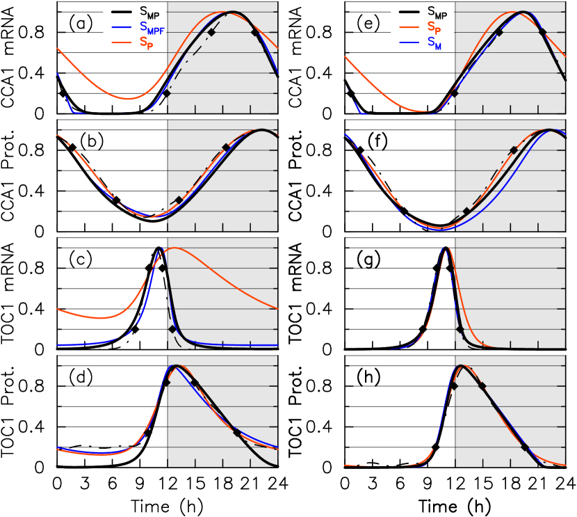
Figure 4: (Color figure) Adjustement of numerical solutions of the free-running model with FRP equal to 24 h (solid lines) to target curves (dash-dotted lines) using various score functions. Panels (a)-(d) in left column show adjustment of mRNA and protein profiles without bias correction, using score functions $S_{MP}$ (black solid line), $S_{MPF}$ (dark grey - blue thin solid line) and $S_{P}$ (light grey or red thin solid line). See text for the definition of score functions. Panels (e)-(h) in right column show adjustment of mRNA and protein profiles with protein floor level removed, using score functions $S_{MP}$ (black solid line), $S_{P}$ (light grey - red thin solid line) and $S_{M}$ (dark grey or blue thin solid line). (a), (e): CCA1 mRNA; (b), (f) CCA1 protein; (c), (g) TOC1 mRNA; (d), (h) TOC1 protein.

Table 1: Model parameter values. Optimal parameter values for adjustement of model to data using various score functions, assuming a free-running period of $24$ hours. Parameters are rescaled so that the maximum value of protein profiles is 100 nM, the maximum value of CCA1 (resp., TOC1) mRNA profile is 10 nM (resp., 70 nM). The TOC1 and CCA1 mRNA maximum values are chosen in the same proportion as in microarray data. The third row of the table indicates whether the floor levels of luminescence data are removed (R) or not (NR). The last part of the table gives the degradation rate $D_{X}$ at the mean value $\bar{X}=\left(\max(X)+\min(X)\right)/2$ ; $D_{x}=\delta_{X}K_{X}/\left(K_{X}+\bar{X}\right)$ for each species.

		$S_{MP}$	$S_{MPF}$	$S_{P}$	$S_{M}$	$S_{MP}$	$S_{P}$
score	(min)	37.7	32.8	12.9	4.2	22.7	11.3
Floor level		NR	NR	NR	R/NR	R	R
$n_{C}$		2	2	1	2	2	2
$n_{T}$		2	2	2	2	2	2
$\mu_{C}$	(nM.$\textrm{h}^{-1}$)	1.92 $10^{-3}$	1.21 $10^{-3}$	5.18 $10^{-3}$	2.97 $10^{-4}$	1.53 $10^{-1}$	1.46 $10^{-1}$
$\lambda_{C}$	(nM.$\textrm{h}^{-1}$)	3.64	6.61	6.56	3.32	3.11	3.31
$P_{T0}$	(nM)	31.6	27.0	91.6	18.8	18.7	50.0
$\beta_{C}$	($\textrm{h}^{-1}$)	2.60	2.50	3.56	2.89	2.83	3.78
$\mu_{T}$	(nM.$\textrm{h}^{-1}$)	0.0117	104	1.69	1.48	0.467	0.0270
$\lambda_{T}$	(nM.$\textrm{h}^{-1}$)	560	3130	67.0	272	487	233
$P_{C0}$	(nM)	7.29	5.65	8.74	3.33	4.51	2.73
$\beta_{T}$	($\textrm{h}^{-1}$)	0.667	0.682	6.86	0.811	0.812	0.759
$1/\delta_{M_{C}}$	(h)	0.542	0.0223	0.831	0.0161	0.195	0.652
$1/\delta_{P_{C}}$	(h)	3.17	4.78	1.51	1.17	2.36	1.44
$1/\delta_{M_{T}}$	(h)	0.140	0.0215	4.97	0.151	0.129	0.736
$1/\delta_{P_{T}}$	(h)	0.559	4.20	0.0659	0.118	0.199	1.65
$K_{M_{C}}$	(nM)	1.35	0.105	2.24	0.0315	0.407	0.842
$K_{P_{C}}$	(nM)	133	746	77.5	23.6	75.9	72.2
$K_{M_{T}}$	(nM)	37.7	12.2	128	60.5	28.3	157
$K_{P_{T}}$	(nM)	7.77	311	45.7	1.52	2.76	47.6
$D_{M_{C}}$	($\textrm{h}^{-1}$)	0.220	0.466	0.220	0.196	0.201	0.119
$D_{P_{C}}$	($\textrm{h}^{-1}$)	0.180	0.185	0.290	0.164	0.183	0.292
$D_{M_{T}}$	($\textrm{h}^{-1}$)	2.49	6.92	0.130	3.08	2.23	0.939
$D_{P_{T}}$	($\textrm{h}^{-1}$)	0.129	0.180	4.76	0.127	0.135	0.196

A first remark is that although a set of four passage times is a very crude description of a temporal profile, it turns out that numerical solutions and experimental profiles that have close passage times generally follow each other closely all over the day. This is consistent with the hypothesis that experimental data are well described by a low-dimensional ODE set. Secondly, the quality of the adjustment is globally very good given the simplicity of the model. Clearly, Fig. 4 shows that Eqs. (1) can adjust simultaneously the protein profiles reconstructed from luminescence time series and the RNA profiles reconstructed from microarray data (score functions $S_{MP}$ and $S_{MPF}$). Especially, removing the protein profile floor levels so as to correct for the detected experimental bias leads to impressive agreement between numerical and target curves, which almost superimpose onto each other.

It is interesting to look more closely at the main discrepancies in Figs 4(a)-(d). When only passage times are taken into account (score function $S_{MP}$), the nonzero floor level of the TOC1 protein is not reproduced. This issue can be addressed by using a score function that takes into account floor level error (score function $S_{MPF}$). In this case, the floor level agreement is improved, at the cost of slightly advancing the protein peak and of inducing a small floor level for TOC1 mRNA. Although small, the latter is definitely much higher than the value that can be accurately determined from microarray data (which estimate the logarithm of mRNA concentration). Last, the numerical solution obtained by adjusting the protein profiles alone (score function $S_{P}$) predicts mRNA profiles rather poorly (Fig. 4), which could suggest that the two types of data are inconsistent.

To an uninformed mind, these minor discrepancies would most probably suggest shortcomings of model (1), not surprisingly given its caricatural simplicity, or the fact that microarray and luminescence data have been recorded in different experiments. However, these discrepancies are clearly linked to errors in floor level, which are naturally explained by the protein floor level bias discussed in Sec. II.3 and evidenced in Fig. 3.

Let us now consider more closely adjustment of model (1) to protein target profiles with floor levels removed, together with RNA target profiles, shown in Figs. 4(e)-(h). Goodness of fit is clearly improved compared to Figs 4(a)-(d), where it was already good. The simultaneous adjustment of the four target curves (score function $S_{MP}$) is achieved with an accuracy rarely obtained for a genetic circuit, with all numerical curves superimposing perfectly on the experimental ones, except that the numerical CCA1 protein profile rises slightly more slowly than the experimental one between dusk and CCA1 expression peak. It is quite striking to note that the two curves begin to separate precisely in the time interval where a transient window of CCA1 stabilization was predicted to occur in Ref. Thommen et al. (2010). Remarkably, numerical profiles obtained by adjusting RNA data alone (score function $S_{M}$) reproduce all experimental data very well also. When protein data are adjusted separately (score function $S_{P}$), RNA profiles are much better reproduced than when the protein floor is not removed, with only the CCA1 mRNA profile showing noticeable discrepancies in certain parts of the day, but with the global shape of the profile preserved. Thus we can conclude that removing floor level significantly improves adjustment and restores coherence between microarray and luminescence data. Given the simplicity of the model, it is very unlikely that this may have occurred by chance. As we will discuss in the next section, it is moreover a remarkable finding that experimental data recorded with different techniques and in different experiments Moulager et al. (2007); Corellou et al. (2009) can be adjusted simultaneously with such high accuracy by a minimal model. This certainly reveals an important property of the clock oscillator.

The parameter sets in the last three columns of Table 1, which correspond to profiles with protein floors removed, are generally more consistent between themselves than those in the first three columns, where the bias has not been corrected, and where important variations can be seen (compare for example $\lambda_{T}$ across the first three columns). This reflects the fact that when the floor level is not removed, it is more difficult to predict mRNA profiles from adjusting protein profiles alone and vice versa. To make meaningful comparisons, it should however be kept in mind that the significant quantities are often not parameters themselves but combinations of them. When degradation is saturated, for example, the relevant quantity is the product $\delta_{X}K_{X}$, and it may happen that $\delta_{X}$ and $K_{X}$ fluctuate more between columns than their product. Therefore, we give at the bottom of Table 1 the effective degradation rates at a mean value of the concentration $D_{X}$, which appear to be much more consistent than the individual degradation parameters. Another example is that although the values of $\mu_{t}$ in the fourth and fifth columns are quite different, the minimum values taken by TOC1 transcription rate in both cases are in fact comparable (1.78 vs 1.45 nM/h), and result from different combinations of $\lambda_{T}$, $P_{C_{0}}$, and of the minimal value reached by the $P_{C}$ profile, which is very close to the repression threshold $P_{C_{0}}$. This illustrates the general fact that although collective fitting can provide well-constrained predictions (here the time profiles), individual parameters may be poorly constrained, a feature observed in many systems biology models Gutenkunst et al. (2007).

Some key ingredients of the dynamics can still be extracted unambiguously from a careful examination of Table 1. The first are the strongly saturated degradations of $M_{C}$ and $P_{T}$, characterized by values of $K_{M_{C}}$ and $K_{P_{T}}$ so small that the concentrations of the respective molecular actors are well above them for almost all of the diurnal cycle. The signature of this behavior in the time profiles is a straight-line decay after the expression peak. A natural question is whether what appears as saturated degradation of a given actor may in fact result from an interaction with another actor not yet identified. In the case of TOC1, a post-transcriptional regulation acting after dusk has indeed been evidenced experimentally Djouani-Tahri et al. (2010). Other key features are a maximum transcription rate significantly higher for TOC1 than for CCA1 and a small threshold of repression $P_{C_{0}}$, comparable to the minimum value of the CCA1 protein level. These are related since the latter implies that TOC1 is repressed most of the time except in a very narrow time interval around the minimum of CCA1 protein level (this correlates with the narrow TOC1 mRNA peak). This must be compensated for by a high TOC1 transcription rate. Interestingly, the small value for $P_{C_{0}}$ can account for the experimentally observed relative inefficiency of antisense strategies against CCA1 Corellou et al. (2009). If CCA1 level is reduced, even significantly, the small time interval where TOC1 is not repressed will extend only slightly, with the dynamical behavior at other times being mostly unchanged. Thus the global perturbation will remain limited and arrhythmia will be difficult to induce. In contrast to this, the activation threshold $P_{T_{0}}$ above which TOC1 activates CCA1 is relatively low so that activation occurs over a rather large time interval of more than 10 hours. Therefore, modifications of the activation threshold or TOC1 protein level will influence the dynamics for a long time and thus easily disrupt oscillations. This also explains why FRP is much more sensitive to overexpression of TOC1 induced by TOC1:luc insertion than of CCA1 induced by CCA1:luc Corellou et al. (2009).

Finally, we carried out data adjustment assuming free-running periods of 23.8 and 25 hours, to verify that our results do not depend critically on FRP (Fig. 5, parameters given in Table 2). In this case, we allowed day/night modulation of some parameters to ensure frequency locking with the diurnal cycle. The agreement remains very good, although it degrades noticeably compared to the case of a FRP of 24 hours. In particular, a phase shift of the TOC1 mRNA profile is induced. The parameter modulation remains very small (for a FRP of 25 hours, the repression threshold is modulated but remains below the minimum of the CCA1 temporal profile, so that the effect of the change is minimal). We furthermore observed that when the FRP was a freely adjustable parameter, it would systematically converge towards a value of 24 hours. All this confirms that there is no day/night parameter modulation in the TOC1–CCA1 feedback loop and that coupling can only occur in specific time windows as proposed in Thommen et al. (2010).

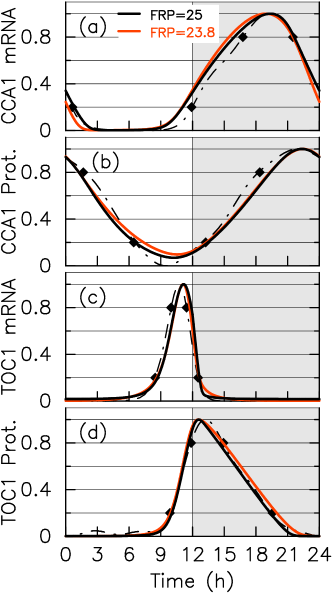
Figure 5: (Color figure) Adjustement of numerical solutions of the light-dependent model (solid lines) to target curves with floor levels removed (dash-dotted line) using the $S_{MP}$ score function. Adjustment of CCA1 mRNA (a), CCA1 protein (b), TOC1 mRNA (c), TOC1 protein (d) without the floor level of proteins. The FRP of the autonomous oscillator is either of 25 h (black solid line) and 23.8 h (light grey or red solid line). Synchronization is obtained for the 25 h (resp., 23.8 h) FRP model by assuming that the parameter $P_{C0}$ (resp., $\delta_{P_{C}}$) take a different value on the day and night.

Table 2: Model parameter values. Optimal parameter values for adjustement of model to data using various score functions and assuming a free-running period of $25$ or $23.8$ hours. Parameters are rescaled as in Table 1

FRP	(h)	25	23.8
score	(min)	27.8	34.3
$n_{C}$		1	1
$n_{T}$		2	2
$\mu_{C}$	(nM.$\textrm{h}^{-1}$)	6.06 $10^{-4}$	4.73 $10^{-2}$
$\lambda_{C}$	(nM.$\textrm{h}^{-1}$)	3.82	4.99
$P_{TO}$	(nM)	15.9	27.3
$\beta_{C}$	($\textrm{h}^{-1}$)	2.71	2.34
$\mu_{T}$	(nM.$\textrm{h}^{-1}$)	22.7	6.07 $10^{-2}$
$\lambda_{T}$	(nM.$\textrm{h}^{-1}$)	357	1130
$P_{C0}$	(nM)	5.94	6.15
$P_{C0}^{\textrm{night}}$	(nM)	11.3
$\beta_{T}$	($\textrm{h}^{-1}$)	0.805	0.809
$1/\delta_{M_{C}}$	(h)	0.305	0.296
$1/\delta_{P_{C}}$	(h)	2.28	2.50
$1/\delta_{P_{C}}^{\textrm{night}}$	(h)		2.60
$1/\delta_{M_{T}}$	(h)	4.28 $10^{-2}$	4.51 $10^{-2}$
$1/\delta_{P_{T}}$	(h)	0.224	0.402
$K_{M_{C}}$	(nM)	0.690	0.879
$K_{P_{C}}$	(nM)	68.5	58.3
$K_{M_{T}}$	(nM)	6.96	17.1
$K_{P_{T}}$	(nM)	3.23	5.62

IV Discussion and Conclusion

In this work, we have carried out a careful and detailed analysis of time series characterizing temporal variations of expression of the two central genes of Ostreococcus circadian clock, TOC1 and CCA1 Corellou et al. (2009). These time series had been previously obtained from microarray data and luminescent reporter data recorded in two different experiments Moulager et al. (2007); Corellou et al. (2009). From these time series, we have extracted periodic temporal profiles for the RNA and protein concentrations of the two genes, assumed to represent the mean circadian oscillations in individual cells so as to optimize comparison with numerical profiles, which are inherently periodic. In particular, approximating the periodic component of luminescence time series by a Fourier series allowed us to separate the dynamics at work throughout the day from fast transient processes activated only near light/dark and dark/light transitions, and probably involved in occasional resetting of the clock (compare raw data and target profile in Fig. 2). The data processing also allowed us to detect a bias in the luminescence time series, which was confirmed by a direct comparison of individual signals from two genetically identical cell cultures (they were not proportional to each other). This bias manifests itself in a nonzero luminescence floor level. Taking it into account allowed us to show that both protein levels approach zero at some times of the day, which was essential for the quality of the subsequent model adjustment. This illustrates how important it is to exploit the redundancy of data by verifying that data that should provide the same information are indeed consistent.

Thanks to the careful data processing, we could evidence an extraordinarily good agreement between a minimal model of a two-gene transcriptional feedback loop and the reconstructed concentration profiles. This model describes activation of CCA1 by TOC1 and repression of TOC1 by CCA1. It describes only regulated transcription of the two genes, translation and degradation, and comprises only differential equations, from which the time evolution of the two mRNA and the two proteins can be computed and compared to the target profiles. Therefore a biochemically detailed model taking into account compartmentalization or genomic insertions would have only served to adjust details without biological relevance, and could well have masked one of the main results which is the good adjustment by a free-running oscillator model. It is also quite remarkable that using only four points of the reconstructed profiles sufficed to constrain the numerical profiles to follow their targets throughout the day. Here also, adding more points would have only forced the model to adjust to unrelevant details without gaining information. This suggests that the complexity of the model and the constraining data should be carefully matched.

The excellent agreement found between the model and the data supports unambiguously the existence of a two-gene oscillator at the core of Ostreococcus circadian clock. This not only builds a solid foundation on which future studies of this clock can rely but also provides what we believe is one of the clearest examples of a natural few-gene oscillator evidenced from experimental data. This is all the more important as the role of this oscillator in the circadian clock constrains it to be extremely robust to all kinds of fluctuations. Understanding the dynamical ingredients besides transcriptional regulation that underlie its robustness will certainly be of high interest for the study of genetic oscillators in general. Two remarkable features of the TOC1–CCA1 oscillator have indeed emerged from our analysis. First, a strongly saturated degradation has been evidenced both for the CCA1 mRNA (already noted in our previous work Thommen et al. (2010)) and the TOC1 protein (detected in this work), which manifests itself by a straight-line decay at high concentrations after the expression peak. This behavior may be the signature of post-transcriptional and post-translation interactions, and is thus compatible with the experimental observations of Ref. Djouani-Tahri et al. (2010). It also supports the putative role of saturated degradation mechanisms as an efficient mechanism to introduce effective delays along a negative feedback loop Kurosawa and Isawa (2002); Tiana et al. (2007); Wong, Tsai, and Liao (2007); Morant et al. (2009) and the recent observation that this is a key ingredient to generate robust oscillations Stricker et al. (2008); Mather et al. (2009). The second remarkable feature predicted by the model is that the TOC1 gene is repressed by CCA1 during most of the day, except during a short time interval located one or two hours before dusk, which is consistent with the very narrow peak of TOC1 mRNA expression observed in the experimental data. The small duration of TOC1 expression is compensated by a high transcription rate. One may wonder whether this design has an influence on the robustness to molecular fluctuations. In any case, it explains why functional studies of the oscillator showed that it was much more sensitive to pertubations in the TOC1 level than in the CCA1 level Corellou et al. (2009).

It has been recently been proposed that circadian clocks should not only be robust to fluctuations in molecule numbers Barkai and Leibler (2000); Gonze, Halloy, and Goldbeter (2002) and to temperature variations Pittendrigh (1954); Rensing and Ruoff (2002) but also to fluctuations in the daylight intensity pattern, which is crucial to synchronize the circadian clock to the day/night cycle Troein et al. (2009); Thommen et al. (2010). Our results demonstrate such robustness for the TOC1–CCA1 oscillator in two different ways. First, the experimental data are reproduced accurately by a free-running oscillator model. This had already been noted by Thommen et al. (2010), but the confirmation of this behavior using luminescence signals recorded every hour reinforces its plausibility significantly. As shown in Thommen et al. (2010), it can only be explained by assuming that coupling to light is scheduled so as to be active precisely when the oscillator does not respond to external perturbations. In this scheme, the oscillator is not affected by light in normal entrainment conditions, which naturally makes it blind to light fluctuations, and thus behaves as if it was free-running. When the oscillator drifts out of phase, light sensing occurs at a different time of its cycle, where it responds so as to recover the normal entrainment phase. The acute responses to light/dark and dark/light transitions that occur transiently in raw signals (Fig. 2) may be correspond to such resetting.

The second strong evidence for the robustness of the TOC1–CCA1 oscillator comes from the fact that the profiles adjusted precisely and simultaneously by our simple model are reconstructed from time series recorded in different experiments by two different techniques, with totally different setups and in particular under very different lighting conditions. This strongly suggests that Ostreococcus clock is able to tick exactly in the same way in different conditions, and in particular in different levels of light, which is an obvious requisite for robustness to daylight fluctuations. If the clock can cope with randomly varying daylight profiles without being perturbed, it can certainly accomodate constantly low or constantly high daylight levels and deliver similar biochemical signals in both cases. The fact that the model adjusted from RNA profiles predicts protein profiles and vice versa (although with less precision in the latter case) clearly illustrates the consistency between the two experiments. Again, we stress that this remarkable finding may have remained masked without our careful data processing.

It is important to mention that both the presence of saturated degradation kinetics and the absence of effective coupling to light when entrained are strong predictions that can be tested experimentally.

While the impressive agreement between model and experiments obtained here clearly shows that a TOC1–CCA1 oscillator underlies Ostreococcus clock, it should not make us forget that it is only a part of it. The free-running average behavior in entrainment conditions, the acute responses at day/night and night/day transitions can only be explained if the TOC1–CCA1 loop interacts with other molecular loops and feedback loops. Indeed it was shown in Thommen et al. (2010) that robustness to daylight fluctuations involves a precisely timed coupling activation. This necessarily requires additional feedback loops designed so as to generate the signal that will drive optimal coupling. Furthermore, interactions with other molecular actors may well be responsible for the saturated degradation of CCA1 mRNA and TOC1 protein.

We thus have now to identify these additional feedback loops as well as the light input pathways, which should help us to understand how the clock can synchronize in spite of fluctuations to day/night cycles of variable duration across the year. Adapting to different photoperiods and to different light levels are indeed unrelated evolutionary goals that must be simultaneously satisfied. In the end, we hope to build an accurate and comprehensive model of a simple and robust circadian clock. If the agreement between theory and experiment remains comparable to what was achieved in the present study, this may well provide us with new and deep insights into the design and function of circadian clocks. More generally, we believe our results promote Ostreococcus, whose low genomic redundancy E. Derelle et al. (2006) is probably crucial for allowing accurate quantitative approaches, as a very promising model for systems biology.

V ACKNOWLEDGMENTS

This work has been supported by ANR grant 07BSYS004 to F-Y.B. and M.L., by CNRS interdisciplinary programme “Interface Physique, Biologie et Chimie: soutien à la prise de risque” to M.L., as well as by French Ministry of Higher Education and Research, Nord-Pas de Calais Regional Council and FEDER through Contrat de Projets Etat-Region (CPER) 2007–2013.

References

- Corellou et al. (2009) F. Corellou, C. Schwartz, J.-P. Motta, E. B. Djouani-Tahri, F. Sanchez, and F.-Y. Bouget, Plant Cell 21, 3436 (2009).
- Thommen et al. (2010) Q. Thommen, B. Pfeuty, P. Morant, F. Correlou, F. Bouget, and M. Lefranc, Plos Comput. Biol. 6, e1000990. doi:10.1371/journal.pcbi.1000990 (2010).
- Goldbeter (1996) A. Goldbeter, Biochemical Oscillations and Cellular Rhythms (Cambridge University Press, Cambridge, 1996).
- Hasty, Hoffmann, and Golden (2010) J. Hasty, A. Hoffmann, and S. Golden, Curr. Opin. Genet. Dev. 20, 571 (2010).
- Winfree (2001) A. T. Winfree, The Geometry of Biological Time, 3rd ed. (Springer Verlag, Berlin, 2001).
- Young (1993) M. W. Young, ed., Molecular Genetics of Biological Rhythms (Dekker, New York, 1993).
- Elowitz and Leibler (2000) M. Elowitz and S. Leibler, Nature 403, 335 (2000).
- Stricker et al. (2008) J. Stricker, S. Cookson, M. R. Bennett, W. H. Mather, L. S. Tsimring, and J. Hasty, Nature 456, 516 (2008).
- Hartwell et al. (1999) L. Hartwell, J. Hopfield, S. Leibler, and A. Murray, Nature 402, 47 (1999).
- Tiana et al. (2007) G. Tiana, S. Krishna, S. Pigolotti, M. H. Jensen, and K. Sneppen, Phys. Biol. 4, R1 (2007).
- Mengel et al. (2010) B. Mengel, A. Hunziker, L. Pedersen, A. Trusina, M. H. Jensen, and S. Krishna, Curr. Opon. Genet. Dev. 20, 656 (2010).
- Rand et al. (2004) D. A. Rand, B. V. Shulgin, D. Salazar, and A. J. Millar, J. R. Soc. Interface 1, 119 (2004).
- Pittendrigh (1960) C. S. Pittendrigh, Cold Spring Harb. Symp. Quant. Biol. 25, 159 (1960).
- Dodd et al. (2005) A. N. Dodd, N. Salathia, A. Hall, E. Kevei, R. Toth, F. Nagy, J. Hibberd, A. J. Millar, and A. A. Webb, Science 309, 630 (2005).
- Moulager et al. (2007) M. Moulager, A. Monnier, B. Jesson, R. Bouvet, J. Mosser, C. Schwartz, L. Garnier, F. Corellou, and F.-Y. Bouget, Plant Physiol. 144, 1360 (2007).
- Monnier et al. (2010) A. Monnier, S. Liverani, R. Bouvet, B. Jesson, J. Smith, J. Mosser, F. Corellou, and F. Bouget, BMC Genomics 11, 192 (2010).
- Gonze, Halloy, and Goldbeter (2002) D. Gonze, J. Halloy, and A. Goldbeter, Proc. Nat. Acad. Sci. USA 99, 673 (2002).
- Barkai and Leibler (2000) N. Barkai and S. Leibler, Nature 403, 267 (2000).
- Pittendrigh (1954) C. S. Pittendrigh, Proc. Natl. Acad. Sci. USA 40, 1018 (1954).
- Rensing and Ruoff (2002) L. Rensing and P. Ruoff, Chronobiol. Int. 19, 807 (2002).
- Comas et al. (2008) M. Comas, D. Beersma, R. Hut, and S. Daan, J. Biol. Rhythms 23, 425 (2008).
- Beersma, Daan, and Hut (1999) D. G. M. Beersma, S. Daan, and R. A. Hut, J. Biol. Rhythms 14, 320 (1999).
- Troein et al. (2009) C. Troein, J. C. W. Locke, M. S. Turner, and A. J. Millar, Current Biology 19, 1961 (2009).
- Dunlap (1999) J. C. Dunlap, Cell 96, 271 (1999).
- Young and Kay (2001) M. W. Young and S. Kay, Nature Genetics 2, 702 (2001).
- Panda, Hogenesch, and Kay (2002) S. Panda, J. B. Hogenesch, and S. A. Kay, Nature 417, 329 (2002).
- Forger and Peskin (2003) D. B. Forger and C. S. Peskin, Proc. Nat. Acad. Sci. USA 100, 14806 (2003).
- Forger et al. (2003) D. B. Forger, D. A. Dean II, K. Gurdziel, J.-C. Leloup, C. Lee, C. Von Gall, J.-P. Etchegaray, R. E. Kronauer, A. Goldbeter, C. S. Peskin, M. E. Jewett, and D. R. Weaver, OMICS 7, 387 (2003).
- Locke et al. (2005) J. C. W. Locke, M. M. Southern, L. Kozma-Bognár, V. Hibberd, P. E. Brown, M. S. Turner, and A. J. Millar, Mol. Syst. Biol. 1, 2005.0013 (2005).
- Locke et al. (2006) J. C. W. Locke, L. Kozma-Bognar, P. D. Gould, B. Feher, E. Kevei, F. Nagy, M. S. Turner, A. Hall, and A. J. Millar, Mol. Syst. Biol. 2, 59 (2006).
- Zeilinger et al. (2006) M. N. Zeilinger, E. M. Farre, S. R. Taylor, and S. A. Kay, Mol. Syst. Biol. 2, 58 (2006).
- Salazar et al. (2009) J. D. Salazar, T. Saithong, P. E. Brown, J. Foreman, J. C. W. Locke, K. J. Halliday, I. A. Carr , D. A. Rand, and A. J. Millar, Cell 139, 1170 (2009).
- François (2005) P. François, Biophys. J. 88, 2369 (2005).
- Courties et al. (1994) C. Courties, A. Vaquer, M. Troussellier, J. Lautier, M. J. Chretiennot-Dinet, J. Neveux, M. C. Machado, and H. Claustre, Nature 370, 255 (1994).
- Chretiennot-Dinet et al. (1995) M. J. Chretiennot-Dinet, C. Courties, A. Vaquer, J. Neveux, H. Claustre, J. Lautier, and M. C. Machado, Phycologia 4, 285292 (1995).
- E. Derelle et al. (2006) E. Derelle et al., Proc. Nat. Acad. Sci. USA 103, 11647 (2006).
- Djouani-Tahri et al. (2010) E. Djouani-Tahri, J.-P. Motta, F.-Y. Bouget, and F. Corellou, Plant Signal Behav. 5, 332 (2010).
- Alabadi et al. (2001) D. Alabadi, T. Oyama, M. J. Yanovsky, F. G. Harmon, P. Mas, and S. A. Kay, Science 293, 880 (2001).
- Gates and DeLuca (1975) B. Gates and M. DeLuca, Arch Biochem Biophys 169, 616 (1975).
- Lefranc, Hennequin, and Glorieux (1992) M. Lefranc, D. Hennequin, and P. Glorieux, Phys. Lett. A 163, 269 (1992).
- Letellier and Aguirre (2010) C. Letellier and L. A. Aguirre, Phys. Rev. E 82, 016204 (2010).
- Gutenkunst et al. (2007) R. N. Gutenkunst, J. J. Waterfall, F. P. Casey, K. S. Brown, C. R. Myers, and J. P. Sethna, PLoS Comput. Biol. 3, e189 (2007).
- Kurosawa and Isawa (2002) G. Kurosawa and Y. Isawa, J. Biol Rhythms 17, 568 (2002).
- Wong, Tsai, and Liao (2007) W. W. Wong, T. Y. Tsai, and J. C. Liao, Mol. Syst. Biol. 3, 130 (2007).
- Morant et al. (2009) P.-E. Morant, Q. Thommen, F. Lemaire, C. Vandermoere, B. Parent, and M. Lefranc, Phys. Rev. Lett. 102, 068104 (2009).
- Mather et al. (2009) W. Mather, M. R. Bennett, J. Hasty, and L. S. Tsimring, Phys. Rev. Lett. 102, 068105 (2009).