SPIN-CURRENTS AND SPIN-PUMPING FORCES FOR SPINTRONICS

Abstract

A general definition of the Spintronics concept of spin-pumping is proposed as generalized forces conjugated to the spin degrees of freedom in the framework of the theory of mesoscopic non-equilibrium thermodynamics. It is shown that at least three different kinds of spin-pumping forces and associated spin-currents can be defined in the most simple spintronics system; the Ferromagnetic/Non-Ferromagnetic metal interface. Furthermore, the generalized force associated to the ferromagnetic collective variable is also introduced in an equal footing, in order to describe the coexistence of the spin of the conduction electrons (paramagnetic spins attached to $s$-band electrons) and the ferromagnetic-order parameter. The dynamical coupling between these two kinds of magnetic degrees of freedom is presented, and interpreted in terms of spin-transfer effects.

I Introduction

Spintronics is a generalization of electronics that takes into account the degrees of freedom related to the spins of the conduction electrons (or the spin of other electric carriers). A typical spintronics system is defined by a statistical ensemble of a plurality of electronic populations (discriminated by their internal degrees of freedom), that are put out of equilibrium in the presence of electric and magnetic forces. The consequence is the creation of currents of electric-charge carriers and currents of spins. Spintronics emerged with the discovery of giant magnetoresistance in the late 80s Nobel_lecture , and it plays today a crucial role in the development of new electronic devices and functionalities.

The goal of this report is revisiting spintronics on the basis of the theory of Non-Equilibrium Thermodynamics DeGroot ; Prigogine ; Stueckelberg ; Smith ; Parrott . The analysis is based on the first and second law of thermodynamics, i.e. on the expression of the power dissipated through the different relaxation mechanisms that characterize the system. The description holds at the mesoscopic scales, under the hypothesis of local equilibrium extended to internal degrees of freedom Prigogine0 ; Rubi . This work is restricted to classical systems. The extension to quantum systems, and especially for the definitions related to ”permanent currents” (for which the second law of thermodynamics is inoperative) is beyond the scope of this report Rque .

I.0.1 Longitudinal spin relaxation

The typical system to be investigated is a 1D wire (with $x$ as coordinate) containing a Ferromagnetic/Non-Ferromagnetic metal junction (or a Ferromagnetic/Ferromagnetic metal junction). In the most simple cases it can be described by a statistical ensemble of independent electrons that are defined by an effective mass $m^{*}$, an electric charge $e$, internal degrees of freedom reduced to the spin one half, and a quantization axis (fixed by the magnetization of the ferromagnetic layer). The system can then be reduced to two electronic populations locally represented by a reservoir of conduction electrons of spin up - defined by a chemical potential $\mu_{\uparrow}(x)$ - and a reservoir of conduction electrons of spin down - defined by a chemical potential $\mu_{\downarrow}(x)$. This is called the two spin-channel model.

There are then two different ways to put the system out of equilibrium. (i) Applying an electric field $E_{\updownarrow}=\frac{-1}{e}\,\frac{\partial\mu_{\updownarrow}}{\partial x}$ will create spin-dependent electric currents $J^{e}_{\updownarrow}=\sigma_{\updownarrow}E_{\updownarrow}$ through the wire (where $\sigma_{\updownarrow}$ is the conductivity). (ii) applying an effective magnetic field will put the two spin populations out-of-equilibrium, creating in turn a flux of spins (noted $\dot{\psi}$ here) in the spin configuration space.

However, the striking point is that the two generalized forces, electric and magnetic, are not independent. Applying a voltage difference through the junction generates also a stationary flux of spins $\dot{\psi}$ because the electric field difference $E_{\uparrow}-E_{\downarrow}=\frac{-1}{e}\frac{\partial\Delta\mu}{\partial x}$ is maintained in the junction. The junction produces a non-zero chemical potential difference $\Delta\mu=\mu_{\uparrow}-\mu_{\downarrow}$, that plays the role of an effective magnetic field, or spin-pumping force conjugated to the flux of spins $\dot{\psi}$. The spin flux can also be written $\dot{\psi}=\delta n/\tau$, where $\tau$ is the spin-flip relaxation time and $\delta n=n_{\uparrow}-n_{\downarrow}$ is the density of out-of-equilibrium spins.

As a consequence, applying a voltage difference through the junction generates not only stationary spin-dependent electric currents $J^{e}_{\updownarrow}$ but also the stationary spin flux $\dot{\psi}$.

If $\mathcal{E}(\mathcal{S},n_{\uparrow},n_{\downarrow})$ is the energy density of the system (function of the entropy $\mathcal{S}$ and the density of charge carriers $n_{\uparrow}$ and $n_{\downarrow}$), the following canonical definitions holds: $T\equiv\frac{\partial\mathcal{E}}{\partial\mathcal{S}}$, $\mu_{\updownarrow}\equiv\frac{\partial\mathcal{E}}{\partial n_{\updownarrow}}$ and $\Delta\mu\equiv\frac{\partial\mathcal{E}}{\partial\psi}$. The first relation defines the temperature, the second defines the chemical potential, and the last relation defines the pumping force $\Delta\mu$ as the chemical affinity of the reaction that transforms a conduction electron of spin up into a conduction electron of spin down PRB00 ; Revue .

The power dissipated by the system at fixed temperature reads $Td\mathcal{S}/dt=-J_{\uparrow}E_{\uparrow}-J_{\downarrow}E_{\downarrow}+\dot{\psi}\Delta\mu$, where $d\mathcal{S}/dt$ is internal entropy production. The relation between the generalized force and the generalized flux is imposed by the second law of thermodynamics, $d\mathcal{S}/dt\geq 0$, and is formally expressed by the Onsager relation.

This model has been first proposed by Johnson and Silsbee Johnson , and the introduction of the pumping force $\Delta\mu$ in the context of spin-dependent transport is due to Van Son et al. Wyder , with the description of longitudinal spin-accumulation and giant magnetoresistance at a Ferromagnetic/Non-Ferromagnetic interface. This approach was systematized by T. Valet and A. Fert in 1993, on the basis of the Boltzmann transport equations Valet . The model is presented below (Section III) in the language of non-equilibrium-thermodynamics.

Note that in the Spintonics literature, the term spin-current is devoted to the spin-dependent electric current $\delta J^{e}=J^{e}_{\uparrow}-J^{e}_{\downarrow}$ that flows through the wire, and not to the spin-flux $\dot{\psi}$ that flows though the spin-space (e.g. the so-called ”Bloch sphere”).

I.0.2 Spin precession

However, the description of spin dynamics in the spin-space is not restricted to spin-flip relaxation (i.e. ”longitudinal” spin relaxation) but it is also characterized by precession effects (”transverse spin relaxation”) as described e.g. by the Bloch equation of the paramagnetic resonance or by the Hanle effect measured in semiconductors Appelbaum . The effect of the precession can be taken into account in terms of diffusion of the transverse components of the spin. This generalization was called transverse spin-accumulation Levy ; Dugaev , and was introduced much later in the context of spin-transfer experiments (see below).

As a consequence, there is another way to drive the spins out-of-equilibrium with the use of the transverse spin pumping force $\Delta\mu_{\perp}$ that generates the transverse spin flux $\dot{\psi}_{\perp}$. Also in that case, the application of a potential difference trough the junction gives rise to non-zero $\Delta\mu_{\perp}$, and the transverse spin-polarized current $\delta J_{\perp}=\sigma_{\perp}\frac{\partial\Delta\mu_{\perp}}{\partial x}$ is produced at the interface. The tranverse spin flux can also be expressed in terms of transverse relaxation time $\tau_{\perp}$ with $\dot{\psi}_{\perp}=\delta n_{\perp}/\tau_{\perp}$. These recent developments are presented in Section IV on equal footing with the longitudinal spin - flip.

I.0.3 Band structure and s-d relaxation

Furthermore, beyond the spin internal degrees of freedom, it is important to push the description to a more realistic situation that takes into account the ferromagnetic specificity of the material (and not only the paramagnetic properties of the conduction electrons). Indeed, the out-of-equilibrium magnetization described within the two-channel model is given by $\delta m=g\mu_{B}(n_{\uparrow}-n_{\downarrow})$ (where $\mu_{B}$ is the Bohr magneton and $g$ the Landé factor). This system is paramagnetic. The contribution $\delta m$ to the total magnetization is superimposed to the ferromagnetic collective variable $\vec{M}$ (which is essentially due to the $d$ band electrons Stearns ). In terms of transport properties, the quasi particles $s$ and $d$ are defined by effective masses $m^{*}_{s}$ and $m^{*}_{d}$, i.e. by supplementary internal degrees of freedom that takes into account the coupling to the periodic lattice.

In line with the pioneering works of Mott Mott , we will consider a simple generalization of the two channel model that takes into account the ferromagnetic nature of the $3d$ metals with enlarging the internal degrees of freedom to four electronic populations: the conduction electrons of the $s$ band for up and down spins, and the conduction electrons of the $d$ band for up and down spins. We have then a four-channel model, in which two kinds of spin flux $\dot{\psi}$ and $\dot{\psi}_{sd}$ should be defined for both interband and intraband spin-dependent relaxation. A third kind of pumping force can then be introduced with the interband chemical potential difference $\Delta\mu_{sd}$ MTEP . This is performed in Section V.

I.0.4 Ferromagnetic collective variable

Nevertheless, there is something missing in the above description of a ferromagnetic junction: the ferromagnetic collective variable $\vec{M}$ has not been introduced explicitly. Accordingly, the next section below (Section II) presents a derivation of the equation of the dynamics for the ferromagnetic variable (i.e. the Landau-Lifshitz-Gilbert equation) performed with the introduction of a generalized force $\vec{\nabla}_{\Sigma}\mu^{F}=-\vec{H}_{eff}$ thermodynamically conjugated to the ferromagnetic degrees of freedom ($\mu^{F}$ is the ferromagnetic chemical potential and $\Sigma$ is the magnetic configuration space). The effective magnetic field $\vec{H}_{eff}$ can also legitimately pretend to the appellation ”spin-pumping force”. This generalized ferromagnetic force generates the current $J^{F}$ in the magnetic configuration space.

Yet, many experiments have shown that it is possible to switch the magnetization Tsoi ; EPL ; Albert ; Julie or to generate ferromagnetic entropy Entropy while injecting spin-polarized currents in Ferromagnetic/Non-Ferromagnetic junctions. The corresponding effect - called spin-transfer - shows that the spin-dependent electronic transport coefficients are coupled to the transport coefficient of the ferromagnet. In other terms, the ferromagnetic current generated by $\vec{H}_{eff}$ and the spin-polarized current generated by $\Delta\mu$, $\Delta\mu_{\perp}$, or $\Delta\mu_{sd}$ are coupled.

The dynamical coupling that occurs between the current of spins and the current of ferromagnetic moments is discussed in Sec. VI. It leads to define a spin-transfer effect for all the spin-pumping sources we have previousely identified : longitudinal Heide ; PRB00 ; Revue , transverse Sloncz ; Braatas , and s-d interband relaxation Berger ; PRB08 .

II Introduction of the ferromagnetic degrees of freedom

In this section, we focus on a uniform ferromagnetic moment $\vec{M}=M_{s}\vec{u}_{r}$ defined with radial unit vector $\vec{u}_{r}$ and the magnetization at saturation $M_{s}$. It is called macrospin, in opposition to the microscopic spins attached to atomes or electrons. In order to treat statistically the time dependence of ferromagnetic degrees of freedom $\vec{m}$ contacted to a heat bath, the ergodic property is used. It allows working with a statistical ensemble of a large number of ferromagnetic moments $\vec{m}\pm d\vec{m}$ that defines a surface $\{\theta\pm\theta,\varphi\pm d\varphi\}$ on the sphere $\Sigma$ of radius $M_{s}$. The corresponding density $\rho^{F}(\theta,\varphi)$ is then identified with the statistical distribution of ferromagnetic moments Ciornei . The mean value of the magnetization is $\vec{M}$. The introduction of the density is justified by the nanoscopic size of the magnetic single domain, for which the fluctuations play a major role. To that point of view, the system is mesoscopic. Accordingly Mazur , the ferromagnetic chemical potential takes the general form $\mu^{F}=kT\,ln(\rho^{F})+V^{F}$ where $V^{F}$ is the usual ferromagnetic potential (deduced e.g. from the quasi static hysteresis loops) and the first term accounts for diffusion. On the other hand the current of ferromagnetic moments, $\vec{J}^{F}=\rho^{F}d\vec{u}_{r}/dt$, is confined on the surface of the sphere.

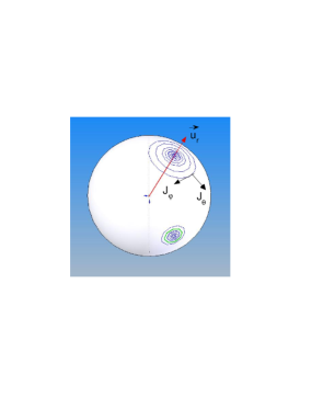
Figure 1: Illustration of the $\Sigma$ configuration space of the ferromagnetic variable. The two potential minima and the ferromagnetic currents are sketched

The power dissipated by the ferromagnetic system is given by the corresponding internal entropy production $\frac{d\mathcal{S}^{F}}{dt}$, and is formed by the product of the generalized flux by the generalized force. Assuming a uniform temperature $T$ we have:

$$T\frac{d\mathcal{S}^{F}}{dt}=-\vec{J}^{F}.\vec{\nabla}_{\Sigma}\mu^{F}$$ (1)

The application of the second law of thermodynamics $d\mathcal{S}^{F}/dt\geq 0$ allows the transport equation to be deduced by writing the relation that links the generalized flux (the current $\vec{J}^{F}$) of the extensive variables under consideration and to the generalized force defined in the corresponding space $\Sigma$. Both quantities, flux and forces, are related by the Onsager matrix of the transport coefficients $\bar{\mathcal{L}}$:

$$\vec{J}^{F}=-\bar{\mathcal{L}}\,\vec{\nabla}_{\Sigma}\mu^{F}$$ (2)

This is the simplest form of the well-known Landau-Lifshitz equation (see below). We started from the hypothesis that the magnetic domain is uniform: the modulus of the magnetization is conserved. The trajectory of the magnetization is then confined on the surface of a sphere of radius $M_{s}$, and the flow is a two component vector defined with the unit vectors $\{\vec{u}_{\varphi},\vec{u}_{\theta}\}$ of $\Sigma$. Accordingly, the Onsager matrix is a 2x2 matrix defined by four transport coefficients $\{L_{\theta\theta},L_{\theta\varphi},L_{\varphi\theta},L_{\varphi\varphi}\}$. Furthermore, the Onsager reciprocity relations impose that $L_{\theta\varphi}=-L_{\varphi\theta}$. Assuming that the dissipation is isotropic, we have $L_{\theta\theta}=L_{\varphi\varphi}$. Let us now introduce a dimensionless supplementary coefficient $\alpha$, which is the ratio of the off-diagonal to the diagonal coefficients: $\alpha=L_{\theta\varphi}/L_{\theta\theta}$. In conclusion, the ferromagnetic kinetic equation is defined by two ferromagnetic transport coefficients $L_{\theta\varphi}=\rho^{F}L_{F}$ and $\alpha$:

$$\bar{\mathcal{L}}=\rho^{F}L_{F}\,\left(\begin{array}[]{cc}\alpha&1\\ -1&\alpha\\ \end{array}\right)$$ (3)

On the other hand, the generalized force $\vec{\nabla}_{\Sigma}\mu^{F}$, thermodynamically conjugated to the magnetization, is the effective magnetic field $\vec{H}_{eff}\equiv-\vec{\nabla}_{\Sigma}\mu^{F}$. It is a generalization in the sense that this effective field includes the diffusive term Raikher that was first introduced by Brown in the rotational Fokker-Planck equation Brown .

Actually, it could be rather surprising to claim that Eq. (2) is the ”well-known LL equation”. However, it is sufficient to rewrite Eq. (2) in 3D space with re-introducing the radial unit vector $\vec{u}_{r}=(1,0,0)$ of the reference frame $\{\vec{u}_{r},\vec{u}_{\theta},\vec{u}_{\varphi}\}$, and recalling that the current is the density multiplied by the velocity $\vec{J}^{F}=\rho^{F}d\vec{u}_{r}/dt$, to recover the traditional LL equation from Eq. (2) and Eq. (3):

$$\frac{d\vec{u}_{r}}{dt}=-L_{F}\,\left\{\vec{u}_{r}\times\vec{H}_{eff}+\alpha\vec{u}_{r}\times\left(\vec{u}_{r}\times\vec{H}_{eff}\right\}\right)$$ (4)

Furthermore, it is well-known that LL equation is equivalent to the phenomenological Gilbert Brown ; Coffey equation, that defines the magnetic damping coefficient $\eta$:

$$\frac{d\vec{M}}{dt}=\gamma\vec{M}\times\left(\vec{H}_{eff}-\eta\,\frac{d\vec{M}}{dt}\right)$$ (5)

where $\gamma$ is the gyromagnetic ratio. The equivalence between the two equations defines the coefficients $\alpha$ and $L_{F}$ as a function of the coefficients $\eta$ and $\gamma$: $\alpha=\eta\gamma M_{s}$ is the dimensionless damping coefficent and $L_{F}$ is defined by the relation:

$$L_{F}=\frac{\gamma}{M_{s}\left(1+\alpha^{2}\right)}$$ (6)

The above approach can be applied to microscopic spins (e.g. for the derivation of the Bloch equation), but it should be generalized to the case in which the modulus of the magnetization is not constant (3 X 3 matrix) and the damping is not necessarily isotrope ($L_{\theta,\theta}\neq L_{\varphi,\varphi}$). This task is beyond the scope of this report.

III Two spin-channel model

In this section, we only focus on the spin-dependent electric transport only, and on the two-channel model sketched in the introduction. The corresponding electric wire is defined along the $x$ axis, with a section unity: the relevant configuration space is the one-dimensional real space $\mathbb{R}$.

The conservation laws write:

$$\left\{\begin{array}[]{c}\frac{dn_{\uparrow}}{dt}\,=\,-\frac{\partial J^{e}_{\uparrow}}{\partial x}-\,\dot{\psi}\\ \frac{dn_{\downarrow}}{dt}\,=\,-\frac{\partial J^{e}_{\downarrow}}{\partial x}+\,\dot{\psi}\\ \end{array}\right.$$ (7)

where $n_{\uparrow}$ and $n_{\downarrow}$ are the densities of charge carriers in the channels $\{\uparrow,\downarrow\}$, and the spin-dependent relaxation is taken into account by the flux $\dot{\psi}$. This is the velocity of the reaction (or relaxation of the spin-dependent internal variable) that transforms a conduction electron $\uparrow$ into a conduction electron $\downarrow$. This relaxation is formally equivalent to a chemical reaction, driven by the chemical affinity $\Delta\mu=\mu_{\uparrow}-\mu_{\downarrow}$ PRB00 . The power dissipated by the system then reads:

$$T\frac{d\mathcal{S}^{e}}{dt}=-J_{\uparrow}^{e}\,\frac{1}{e}\frac{\partial\mu_{\uparrow}^{e}}{\partial x}-J_{\downarrow}^{e}\,\frac{1}{e}\frac{\partial\mu_{\downarrow}^{e}}{\partial x}+\dot{\psi}\Delta\mu$$ (8)

The corresponding kinetic equations are deduced from the second law of thermodynamics, after introducing a supplementary Onsager coefficient $L$.

$$\left\{\begin{aligned} J^{e}_{\uparrow}&=-\frac{\sigma_{\uparrow}}{e}\frac{\partial\mu^{e}_{\uparrow}}{\partial x}\\ J^{e}_{\downarrow}&=-\frac{\sigma_{\downarrow}}{e}\frac{\partial\mu^{e}_{\downarrow}}{\partial x}\\ \dot{\psi}&=L\Delta\mu\end{aligned}\right.$$ (9)

The set of equations Eqs (9) is sufficient and necessary in order to describe, in the stationary regime, spin-accumulation effects and any non-equilibrium contribution to the resistance due to relaxation ($\Delta\mu\neq 0$) occurring at an interface Revue ; MTEP .

Eq. (9) shows that the spin-dependent electric currents $J^{e}_{\updownarrow}$ and the spin flux $\dot{\psi}$ are not independent. Accordingly, it is more convenient to rewrite Eq. (9) as a function of the variables $\Delta\mu$ and $\mu_{0}=\mu_{\uparrow}+\mu_{\downarrow}$. Let us define the conductivity asymmetry by the parameter $\beta$ such that $\beta=\frac{\sigma_{\uparrow}-\sigma_{\downarrow}}{\sigma_{0}}$ and the mean conductivity $2\sigma_{0}=\sigma_{\uparrow}+\sigma_{\downarrow}$. On the other hand, the spin-polarized electric current is $\delta J^{e}=J^{e}_{\uparrow}-J^{e}_{\downarrow}$ and the spin-independent current is $J^{e}_{0}=J^{e}_{\uparrow}+J^{e}_{\downarrow}$. In this new system of equations, the Onsager matrix re-writes:

$$\left(\begin{array}[]{c}\delta J^{e}\\ J^{e}_{0}\\ \dot{\psi}\end{array}\right)=\left(\begin{array}[]{ccc}\sigma_{0}&\beta\sigma_{0}&0\\ \beta\sigma_{0}&\sigma_{0}&0\\ 0&0&L\end{array}\right)\left(\begin{array}[]{c}\frac{-1}{e}\frac{\partial{\Delta{\mu}^{e}}}{\partial{x}}\\ \frac{-1}{e}\frac{\partial\mu^{e}_{0}}{\partial x}\\ \Delta\mu\\ \end{array}\right)$$ (10)

The current $\delta J^{e}$ is called ”spin current” or ”pure spin-current” in the spintronics literature.

The system of equations Eq. (10) allows the diffusion equation for $\Delta\mu(x)$ to be derived for the stationary conditions $\frac{\partial J_{0}^{e}}{\partial x}=0$ and $\frac{\partial\delta J^{e}}{\partial x}=-2\dot{\psi}$:

$$\frac{\partial^{2}\Delta\mu}{\partial x^{2}}=\frac{\Delta\mu}{l^{2}_{diff}}$$ (11)

where $l_{diff}^{-2}=\frac{2eL}{\sigma_{0}(1-\beta^{2})}$. And the non-equilibrium magnetoresistance produced by the interface writes (see the details of the derivation in references Revue ; MTEP ; PRB08 ):

$$R^{ne}=-\frac{2\beta}{J_{0}^{e}e}\int_{A}^{B}\frac{\partial\Delta\mu}{\partial x}dx$$ (12)

where the measurement points $A$ and $B$ are located far enough in each side of the interface so that $\Delta\mu^{e}(A)=\Delta\mu^{e}(B)=0$.

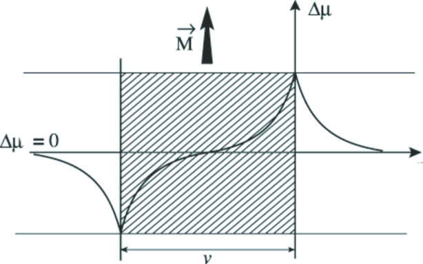
Figure 2: Spin-accumulation $\Delta\mu(x)$ trough a Non-Ferromagnetic/Ferromagnetic/Non-Ferromagntic junction with typical size of the order of the spin diffusion length

The spin diffusion length is typically some tens of nanometers in ferromagnetic metals, so that the non-equilibrium magnetoresistance requires thin films (current-in-plane geometry) or nanostructured pillars (current-perpendicular-to-the-plane geometry) to be exploited.

IV Spin precession

The description proposed above with a spin-dependent internal variable that takes the two spin values $\{\uparrow,\downarrow\}$ is not able to take into account the precession of the spins occurring in a magnetic field, and observed with electronic resonance or Hanle effects. In the case of the processes that lead to spin accumulation and giant magnetoresistance, the mean values are averaged out over the spin-diffusion length, so that the precession of the spin is not relevant. However, this is no longer the case in a quasi-ballistic regime close enough to the interface.

In order to take into account these quasi-ballistic effects (i.e. sub-nanometric scales in metalic devices), the two-channel model has been recently generalized to transverse spin-accumulation in the context of spin-transfer-torque investigations LevyFert ; Levy ; Dugaev . The transverse spin-accumulation is introduced with the corresponding current $\delta J^{e}_{\perp}$ and the corresponding chemical potential $\Delta{\mu}^{e}_{\perp}$. Transverse means here that the spin density is considered in the plan perpendicular to the quantification axis $\updownarrow$ that defines the spin up and spin down in the two-channel model.

The conservation laws writes:

$$\frac{\partial\delta n_{\perp}}{\partial t}=-\frac{\partial J_{\perp}}{\partial x}-\dot{\psi}_{\perp}$$ (13)

The transverse spin flux $\dot{\psi}_{\perp}$ can be expressed with a transverse relaxation time $\tau_{\perp}$: $\dot{\psi}_{\perp}=\frac{\delta n_{\perp}}{\tau_{\perp}}$, where $n_{\perp}$ is the density of transverse spins.

Note that the two potentials $\Delta\mu^{e}$ and $\Delta\mu_{\perp}^{e}$ are defined at very different length scales and it is necessary to refer to quantum approaches in order to understand the physical signification of the transverse parameters Waintal ; Braatas . The corresponding transverse contribution to the dissipated power is

$$T\frac{d\mathcal{S}^{e}_{\perp}}{dt}=-\delta J^{e}_{\perp}\,\frac{\partial\Delta\mu^{e}_{\perp}}{e\partial x}+\dot{\psi}_{\perp}\Delta\mu_{\perp}$$ (14)

Putting all together, we have the following Onsager relations for the electric system:

$$\left(\begin{array}[]{c}\delta J^{e}\\ J^{e}_{0}\\ \delta J^{e}_{\perp}\\ \dot{\psi}\\ \dot{\psi}_{\perp}\end{array}\right)=\left(\begin{array}[]{ccccc}\sigma_{0}&\beta\sigma_{0}&0&0&0\\ \beta\sigma_{0}&\sigma_{0}&0&0&0\\ 0&0&\sigma_{\perp}&0&0\\ 0&0&0&L&0\\ 0&0&0&0&L_{\perp}\end{array}\right)\left(\begin{array}[]{c}\frac{-1}{e}\frac{\partial{\Delta{\mu}^{e}}}{\partial{x}}\\ \frac{-1}{e}\frac{\partial\mu^{e}_{0}}{\partial x}\\ \frac{-1}{e}\frac{\partial{\Delta{\mu}^{e}_{\perp}}}{\partial{x}}\\ \Delta\mu\\ \Delta\mu_{\perp}\\ \end{array}\right)$$ (15)

V The role of the $d\downarrow$ electronic subband

A justification of the spin-dependent conductivity asymmetry $\beta\neq 0$ in ferromagnetic metals has been proposed by N. Mott in 1936 Mott , on the bases of the newly discovered band-structure approach. In the Mott description, the observed transport properties (e.g. the huge resistivity of Ni below the Curie temperature) have been accounted for by the existence of four electronic populations: the conduction electrons of spin up and down ($s\uparrow$ and $s\downarrow$) of the $s$ band and the conduction electrons of spin up and down ($d\uparrow$ and $d\downarrow$) of the $d$ band. The argument is based on the fact that the contribution to the resistivity of the $s-d$ interband scattering is higher than the contribution of the $s$ intraband scattering. In the ferromagnetic 3d metal, the $d\uparrow$ band is full so that the relaxation channel of $s\uparrow$ electrons to $d\uparrow$ band is blocked (according to the Fermi golden rule, the relaxation rate is proportional to the density of states in the final $d\downarrow$ band). Furthermore, the spin-flip interband relaxation is too energetic to be efficient (the relaxation $s\uparrow$ to $d\downarrow$ is negligible). As a consequence, the $s\downarrow$ are more scattered that the $s\uparrow$, and the conductivities of the two channels is asymmetric: $\sigma_{\uparrow}>\sigma_{\downarrow}$. This mechanism is also responsible for the anisotropic magnetoresistance Potter . The necessity of enlarging the internal degrees of freedom to the band structure leads to enrich the concept of spin-currents and the spin-pumping force.

Using the notations introduced in the previous sections, the total current $J_{t}$ is composed by the three currents for each channel : $J_{t}=J_{s\uparrow}+J_{s\downarrow}+J_{d\downarrow}$ ($J_{d\uparrow}=0$ because the band is full). The relaxation rate $\dot{\psi}_{sd}$ is introduced to account for $s-d$ spin-conserved scattering, and the relaxation rate $\dot{\psi}_{s}$, is introduced in order to account for previously defined spin-flip scattering. Assuming that all channels are in steady states, the conservation law write:

$$\left\{\begin{aligned} \frac{\partial n_{t}}{\partial t}&=-\frac{\partial J_{t}}{\partial x}=0\\ \frac{\partial n_{s\uparrow}}{\partial t}\,&=\,-\frac{\partial J_{s\uparrow}}{\partial x}-\,\dot{\psi}_{s}=0\\ \frac{\partial n_{s\downarrow}}{\partial t}\,&=\,-\frac{\partial J_{s\downarrow}}{\partial x}-\,\dot{\psi}_{sd}+\,\dot{\psi}_{s}=0\\ \frac{\partial n_{d\downarrow}}{\partial t}\,&=-\frac{\partial J_{d\downarrow}}{\partial x}+\dot{\psi}_{sd}=0\end{aligned}\right.$$ (16)

where $n_{t},n_{s\uparrow},n_{s\downarrow},n_{d\downarrow}$ are respectively the total densities of particles and the density of particles in the $s\uparrow$, $s\downarrow$, $d\downarrow$ channels. The conjugate (intensive) variables are the chemical potentials $\{\mu_{s\uparrow},\mu_{s\downarrow},\mu_{d\uparrow},\mu_{d\downarrow}\}$. The application of the first and second laws of thermodynamics allows us to deduce the Onsager relations of the system :

$$\left\{\begin{aligned} J_{s\downarrow}&=-\frac{\sigma_{s\downarrow}}{e}\frac{\partial\mu_{s\downarrow}}{\partial x}\\ J_{s\uparrow}&=-\frac{\sigma_{s\uparrow}}{e}\frac{\partial\mu_{s\uparrow}}{\partial x}\\ J_{d\downarrow}&=-\frac{\sigma_{d\downarrow}}{e}\frac{\partial\mu_{d\downarrow}}{\partial x}\\ \dot{\psi}_{sd}&=L_{sd}\left(\mu_{s\downarrow}-\mu_{d\downarrow}\right)\\ \dot{\psi}_{s}&=L_{s}\left(\mu_{s\uparrow}-\mu_{s\downarrow}\right)\end{aligned}\right.$$ (17)

where the conductivity of each channel $\{\sigma_{s\uparrow},\sigma_{s\downarrow},\sigma_{d\uparrow},\sigma_{d\downarrow}\}$ has been introduced. The first four equations are the Ohm’s law applied to each channel, and the two last equations introduce new Onsager transport coefficients, $L_{sd\downarrow}$ and $L_{s}$, that respectively describe the $s-d$ relaxation (I) for minority spins under the action of the chemical potential difference $\Delta\mu_{\downarrow}=\mu_{s\downarrow}/2-\mu_{d\downarrow}$ and the spin-flip relaxation (II) under spin pumping $\Delta\mu_{s}=\mu_{s\uparrow}-\mu_{s\downarrow}/2$. The Onsager coefficients are proportional to the corresponding relaxation times Revue .

In the same manner as performed in Section III, the equations of conservation Eqs. (16) and the Onsager equations Eqs. (17) lead to the two coupled diffusion equations :

$$\left\{\begin{aligned} \frac{\partial^{2}\Delta\mu_{\downarrow}}{\partial x^{2}}\,&=\,\frac{1}{l_{sd}^{2}}\,\Delta\mu_{\downarrow}-\frac{1}{\lambda_{s}^{2}}\Delta\mu_{s}\\ \frac{\partial^{2}\Delta\mu_{s}}{\partial x^{2}}\,&=\,\frac{1}{\lambda_{sd}^{2}}\,\Delta\mu_{\downarrow}-\frac{1}{l_{sf}^{2}}\,\Delta\mu_{s}\end{aligned}\right.$$ (18)

where the four diffusion lengths $\{l_{sd},\lambda_{s},l_{sf},\lambda_{sd}\}$ are given as a function of the transport coefficients in reference Revue .

This three-channel model brings to light the interplay between band mismatch effects and spin accumulation, in a diffusive approach. The resolution of the coupled diffusion equations is discussed elsewhere Revue .

VI Derivation of Spin transfer due to spin-pumping forces

In usual experimental configurations for spin-transfer, an electric current is injected in a ferromagnet through an interface (in series or in non-local configuration Otani ) and the magnetoresistance, i.e. the potential drop Eq. (12) allows the magnetization states to be measured. The effect of strong electric currents on the magnetization states can then be observed. In such a configuration, the two sub-systems $\Sigma$ and the spin-polarized current described in the previous sections exchange magnetic moments at the junctions and both are open systems.

In order to describe the dynamics of the ferromagnetic degrees of freedom, we have to deal with a closed system. The system of interest is now the ferromagnetic system that includes spin-accumulation effects at the junctions.

For the sake of simplicity, we treat in the following a unique decoupled spin-dependent process $\Delta\mu$ and $\dot{\psi}$ that includes $s-d$ relaxation.

This total ferromagnetic system is such that the density of ferromagnetic moments $\rho^{F}_{tot}$ and the total ferromagnetic flux $\vec{J}^{F}_{tot}$ are related by the conservation law: $d\rho^{F}_{tot}/dt=-div_{\Sigma}\vec{J}^{F}_{tot}$.

The initial configuration space of magnetic moments is then extended to 1D real space parametrized by the internal variable $\Sigma\otimes\mathbb{R}_{\Sigma}$. The important point here is that the internal variable is spin dependent, and related to the ferromagnetic space $\Sigma$ (e.g. through spin-flip or $s-d$ relaxation and the corresponding spin accumulation). This accounts for the coupling, i.e. the transfer, of magnetic moments between the two sub-systems.

The dissipation is given by the internal power dissipated in the total system $T\,d\mathcal{S}/dt$ :

$$T\,d\mathcal{S}/dt=-\vec{j}_{tot}^{F}.\vec{\nabla}_{\Sigma}\mu^{F}-\delta J^{e}.\frac{\partial{\Delta{\mu}^{e}}}{e\partial{x}}-\delta J^{e}_{\perp}.\frac{\partial{\Delta{\mu}^{e}_{\perp}}}{e\partial{x}}-J_{0}^{e}\frac{\partial{\mu_{0}^{e}}}{e\partial{x}}+\dot{\psi}\Delta\mu^{e}+\dot{\psi}\Delta\mu^{e}_{\perp}$$ (19)

Where the first term in the right hand side is the power dissipated by the total ferromagnetic sub-system (including the ferromagnetic contribution due to spin-transfer), the two following terms are the power dissipated by spin-dependent electric transport, and the fourth term is the spin-independent Joule heating. The last term is the power dissipated by spin-flip or $s-d$ relaxation.

In Eq. (19), the vectors are defined on the sphere $\Sigma$ with the help of two angles $\theta$ and $\varphi$. The total ferromagnetic current $\vec{j}_{tot}^{F}=j_{tot\,\perp}^{F}\vec{u}_{\varphi}+j_{tot\,//}^{F}\vec{u}_{\theta}$ includes the contribution due to spin-accumulation mechanisms. The chemical potential $\mu^{F}$ accounts for the energy of a ferromagnetic layer. On the other hand, the system is contacted to electric reservoirs with the electric currents and the corresponding chemical potentials. Applying the second law of thermodynamics, we obtain the general Onsager relations:

$$\left(\begin{array}[]{c}j_{tot\,\perp}^{F}\\ j_{tot\,//}^{F}\\ \delta J^{e}_{\perp}\\ \delta J^{e}\\ \dot{\psi}_{\perp}\\ \dot{\psi}\end{array}\right)=\left(\begin{array}[]{cccccc}\rho L_{F}\alpha&\rho L_{F}&l_{\perp}&0&0&0\\ -\rho L_{F}&\rho L_{F}\alpha&0&l_{//}&0&0\\ \tilde{l}_{\perp}&0&\sigma_{\perp}&0&0&0\\ 0&\tilde{l}_{//}&0&\sigma_{0}&0&0\\ 0&0&0&0&\L_{\perp}&0\\ 0&0&0&0&0&L\end{array}\right)\left(\begin{array}[]{c}\frac{1}{sin\theta}\frac{\partial\mu_{\perp}^{F}}{\partial\varphi}\\ \frac{\partial\mu_{//}^{F}}{\partial\theta}\\ \frac{-1}{e}\frac{\partial{\Delta{\mu}^{e}_{\perp}}}{\partial{x}}\\ \frac{-1}{e}\frac{\partial{\Delta{\mu}^{e}}}{\partial{x}}\\ \Delta\mu_{\perp}\\ \Delta\mu\\ \end{array}\right)$$ (20)

All coefficients were defined in the previous sections, except the two cross-coefficients $\{l_{\perp},l_{//}\}$, introduced in this model as spin-transfer coefficients. The coefficients $\{\tilde{l}_{\perp},\tilde{l}_{//}\}$ are given by the Onsager reciprocity relations. We assumed that the other cross-coefficents are zero or negligible.

The total ferromagnetic current can be written after integrating over the volume $v$ of the ferromagnetic layer of section unity and the spin accumulation zone. This volume is such that $v=\int_{A}^{B}dz$, where $x=A$ and $x=B$ are two sections close to the interface but far enough with respect to the diffusion lengths. We assume here that the diffusion lengths are much smaller than the width of the ferromagnetic layer in order to simplify the calculation: the volume of the ferromagnet is identified as $v$. Let us define $\vec{X}$ as the correction due to the spin-transfer after integrating over the volume $v$ deduced from the two first equations of the matrix equation Eq. (20),:

$$\vec{J}_{tot}^{F}=\bar{\mathcal{L}}v\,\vec{\nabla}_{\Sigma}\mu^{F}+\rho\,v\vec{X}$$ (21)

where $\bar{\mathcal{L}}$ is the matrix defined in Eq. (3).

The assumption of constant modulus of the magnetization imposes that $\vec{X}$ is confined on the surface of the sphere $\Sigma$. The Helmoltz decomposition theorem can then be applied: the vector $\vec{X}$ can be decomposed in a unique way with the introduction of two potentials $\chi$ and $\Phi$ (i.e. a potential vector) such that:

$$\vec{X}=\vec{u}_{r}\times\vec{\nabla}_{\Sigma}\Phi+\vec{\nabla}_{\Sigma}\chi$$ (22)

where the first term is divergenceless and the second term is curlless (i. e. non conservative). The total correction to the Landau-Lifshitz-Gilbert equation writes

$$\vec{J}_{tot}^{F}=v\bar{\mathcal{L}}\vec{\nabla}_{\Sigma}\mu^{F}+\vec{\nabla}_{\Sigma}\chi+\vec{u}_{r}\times\vec{\nabla}_{\Sigma}\Phi$$ (23)

The generalized LLG takes the form:

$$\frac{d\vec{u}_{r}}{dt}=-L_{F}\left\{\vec{u}_{r}\times\left(\vec{H}_{eff}-\frac{\vec{\nabla}_{\Sigma}\Phi}{L_{F}}\right)-\alpha\vec{u}_{r}\times\left(\vec{u}_{r}\times\left(\vec{H}_{eff}-\frac{\vec{\nabla}_{\Sigma}{\chi}}{\alpha L_{F}}\right)\right)\right\}$$ (24)

where $\vec{H}_{eff}=-\vec{\nabla}\mu^{F}$ is the usual effective ferromagnetic field.

Eq. (24) is a generalized LLG equation that includes the effect of spin-pumping $\Delta\mu$ and $\Delta\mu_{\perp}$ (the contribution of $\Delta\mu_{sd}$ has not been added to the Onsager relations Eq. (20) for the sake of simplicity). Qualitiatively, the most important point is that the dynamics should now be described by the introduction of two potentials, or two magnetic fields $\vec{H}_{eff}-\frac{\vec{\nabla}_{\Sigma}\Phi}{L_{F}}$ for the precession and $\vec{H}_{eff}-\frac{\vec{\nabla}_{\Sigma}{\chi}}{\alpha L_{F}}$ for the longitudinal relaxation, instead of a single field $\vec{H}_{eff}$ in the usual case. Both fields appearing in the LLG equation contains a current dependence.

The corresponding Fokker-Planck equation is obtained by inserting the expression of $\vec{J}_{tot}$ into the conservation equation: $d\rho^{F}_{tot}/dt=-div_{\Sigma}\vec{J}^{F}_{tot}$.

VII Conclusion

The basic concepts of Spintronics - spin-pumping force and spin currents - have been presented on the basis of the theory of Non-Equilibrium Thermodynamics. It has been shown that different relaxation mechanisms can be invoked, each of which defines a specific spin-pumping force and a specific spin flux. Four mechanisms have been investigated within this formalism: spin-flip scattering, spin precession, $s-d$ scattering, and ferromagnetic relaxation (with both longitudinal relaxation and precessional motion).

This approach shows that the application of a voltage difference through a Ferromagnetic/Non-Ferromagnetic junction leads to the creation of spin-pumping and spin-flux, which in turn leads to non-equilibrium interface resistance or spin-transfer to the ferromagnetic collective variable. The derivation proposed for the spin-accumulation formulae, dynamics of the magnetization, and spin-transfer effects, are based on the expression of the entropy production and the second law of thermodynamics. In principle, it is possible to obtain the same results in a more elegant way, by using the Prigogine s theorem on minimal entropy production. This work rest to be performed.

References

- (1) A. Fert, the origin, development and future of spintronics, Nobel Lecture, The Nobel Prizes 2007, Editor Karl Grandin, [Nobel Foundation], Stockholm, 2008
- (2) S. R. De Groot and P. Mazur, Non-equilibrium thermodynamics Amsterdam : North-Holland, 1962.
- (3) I. Prigogine, Introduction to thermodynamics of irreversible processes, J. Wiley and Sons, Inc., New York, 1962.
- (4) E.C.G. Stueckelberg and P.B. Scheurer, thermocinétique phénoménologique galiléenne Birkauser Verlag, Basel and Stuttgart, 1974.
- (5) A. C. Smith, J. F. Janak, R. B. Adler, Electric conduction in solids, McGraw-Hill Inc 1967, Chapter 1 and Chapter 2.
- (6) J. E. Parrott, Thermodynamic theory of transport processes in semiconductors, IEEE Trans electron devices 43, 809 (1996).
- (7) I. Prigogine, P. Mazur, Physica 19, 241 (1953).
- (8) D. Reguera, J. M. G. Vilar and J. M. Rubí, J. Phys. Chem. B, 109, 21502 (2005).
- (9) A proper quantum definition of the spin-current in the case spin-orbit coupling is an open problem. A clear presentation can be found in E. I. Rashba, Phys. Rev. B 68, 241315(R) (2003) and Phys. Rev. B 70, 161201(R) (2004), and E. B. Sonin, Phys. Rev. B 76, 033306 (2007), Phys. Rev. B 77, 039901 (2008). The discussion is performed in H.-J. Drouhin, G. Fishman, J.-E. Wegrowe, Cond-Mat.
- (10) T.L. Hoai Nguyen, H.-J. Drouhin, J.-E. Wegrowe and G. Fishman, Phys. Rev. B 79, 165204 (2009).
- (11) J. -E. Wegrowe, Phys. Rev. B 62, 1067 (2000).
- (12) J.-E. Wegrowe, M. C. Ciornei, H.-J. Drouhin, J. Phys.: Condens. Matter 19, 165213 (2007).
- (13) Johnson, M.; Silsbee, R. H. Phys. ReV. Lett. 1985, 55, 1790 and Johnson, M.; Silsbee, R. H. Phys. Rev. B (1987), 35, 4959.
- (14) P.C. van Son, H. van Kempen, and P. Wyder, Phys. Rev. Lett. 58, 2271 (1987).
- (15) T. Valet and A. Fert, Phys. Rev. B 48, 7099 (1993).
- (16) N. F. Mott and H. Jones, Theory of the Properties of Metal and Alloys, Chapter VII 6, Oxford University Press, 1953.
- (17) Coherent Spin Transport through 350 Micron Thick Silicon Wafer, B. Huang, D. J. Monsma, and I. Appelbaum, Phys. Rev Lett. 99, 177209 (2007).
- (18) A. Shpiro, S. Zhang, and P M. Levy, Phys. Rev B 67, 104430 (2003), J. Zhang, S. Zhang, V. Antropov, and P. M. Levy, Phys. Rev. Lett. 93, 2566002 (2004) and J. Zhang, P. M. Levy, Phys. Rev. B 71, 184426 (2005).
- (19) V. K. Dugaev, J. Barnas, J. Appl. Phys. 97 023902 (2005).
- (20) M. B. Stearns, On the origine of Ferromagnetism and the Hyperfine FIelds in Fe, Co and Ni, Phys. Rev. B, 6, 4383 (1973).
- (21) J.-E. Wegrowe, Q. Anh Nguyen, M. Al-Barki, J.-F. Dayen, T. L. Wade, and H.-J. Drouhin, Phys. Rev. B 73 134422, (2006).
- (22) M. Tsoi, A.G. M. Jansen, J. Bass, W.-C. Chiang, M. Seck, V. Tsoi, and P. Wyder, Phys. Rev. Lett. 80, 4281 (1998)
- (23) J-E. Wegrowe, D. Kelly, Y. Jaccard, Ph. Guittienne, J-Ph. Ansermet Europhysics letters 45 626 (1999).
- (24) F. J. Albert, J. A. Katine, R. A. Buhrman, and D. C. Ralph, Appl. Phys. Lett. 77 3809 (2000).
- (25) J. Grollier, V. Cros, A. Hamzic, J.M. George, H. Jaffes, A. Fert, G. Faini, J. Ben Youssef, and H. Le Gall, Appl. Phys. Lett. 78, 3663 (2001).
- (26) J. -E. Wegrowe, Q. Anh Nguyen, T. Wade, IEEE Trans. Mag. 45 (2010), 866.
- (27) C. Heide, P.E. Zilberman, and R. Elliott, PRB 63, 064424 (2001); C. Heide, Phys. Rev. LEtt. 87, 197 201 (2001).
- (28) J. C. Slonczewski, J. Magn. Magn. Mat. 159 L1 (1996).
- (29) A. Braatas, G. E. W. Bauer, P. J. Kelly, Phys. Report, 427, 157 (2006).
- (30) L. Berger, J. appl. Phys. 55, 1954 (1984).
- (31) J.-E. Wegrowe, S. M. Santos, M.-C. Ciornei, H.-J. Drouhin and M. Rubi, Phys. Rev. B, 174408 77 (2008).
- (32) M.-C. Ciornei, J. M. Rub and J.-E. Wegrowe, arXiv:1008.2177v1 [cond-mat.mes-hall] 12 Aug 2010
- (33) A statistical justification of this expression of the chemical potential was given by P. Mazur, Physica A 261, 451 (1998).
- (34) Y. L. Raikher and V. I. Stepanov, Adv. Chem. Phys. 129, 419 (2004).
- (35) W. F. Brown Jr., Phys. Rev. 130, 1677 (1963).
- (36) W. T. Coffey, Yu. P. Kalmykov and J. T. Waldron, The Langevin equation, World Scientific Series in contemporary Chemical Physics Vol. 11, 1996.
- (37) S. Zhang, P. M. Levy, and A. Fert, Phys. Rev. Lett. 88, 236601 (2002).
- (38) X. Waintal, E. B. Myers, P. W. Brouwer, D. C. Ralph, Phys. Rev. B 62, 12317 (2000).
- (39) T. R. McGuire and R. I. Potter, IEEE Trans. vol Mag-11, 1018 (1975).
- (40) Kimura, T., Otani, Y. and Hamrle, J., Phys. Rev. Lett. 96, 037201 (2006).