Quirks in supersymmetry with gauge coupling unification

Abstract

I investigate the phenomenology of supersymmetric models with extra vector-like supermultiplets that couple to the Standard Model gauge fields and transform as the fundamental representation of a new confining non-Abelian gauge interaction. If perturbative gauge coupling unification is to be maintained, the new group can be $SU(2)$, $SU(3)$, or $SO(3)$. The impact on the sparticle mass spectrum is explored, with particular attention to the gaugino mass dominated limit in which the supersymmetric flavor problem is naturally solved. The new confinement length scale is astronomical for $SO(3)$, so the new particles are essentially free. For the $SU(2)$ and $SU(3)$ cases, the new vector-like fermions are quirks; pair production at colliders yields quirk-antiquirk states bound by stable flux tubes that are microscopic but long compared to the new confinement scale. I study the reach of the Tevatron and LHC for the optimistic case that in a significant fraction of events the quirk-antiquirk bound state will lose most of its energy before annihilating as quirkonium.

I Introduction

Among the hurdles that must be cleared by any proposed extension of the Standard Model (SM) are the stringent limits on quantum corrections to the electroweak vector boson propagators due to new physics Peskin:1991sw -Altarelli:1990zd . Low-energy supersymmetry primer is generally safe in this regard, because of the fact that all of the new particles it introduces get their masses primarily from bare mass terms, not from their couplings to the Higgs vacuum expectation values (VEVs). This includes the Higgs chiral supermultiplets $H_{u}$ and $H_{d}$ themselves, which are vector-like, together forming a self-conjugate representation of the SM gauge group $G_{\rm SM}=SU(3)_{c}\times SU(2)_{L}\times U(1)_{Y}$. It is therefore interesting to consider non-minimal supersymmetric models that maintain this feature by including more chiral supermultiplets transforming as vector-like representations of the gauge group.

Another well-known and appealing feature of the minimal supersymmetric standard model (MSSM) is the perturbative unification of running gauge couplings near $M_{U}\approx 2\times 10^{16}$ GeV. A sufficient (but not necessary) condition for extensions of the MSSM with extra vector-like supermultiplets to maintain gauge coupling unification is that the new fields come in complete multiplets of the $SU(5)$ global symmetry group that contains $G_{\rm SM}$. This paper studies the properties of models of this type that introduce a new non-Abelian gauge group $G_{X}$, under which the new chiral supermultiplets also transform but the MSSM fields are neutral. Models of this type have already been introduced by Babu, Gogoladze, and Kolda in Babu:2004xg , in the context of finding new large contributions to the lightest Higgs boson mass. I will assume that the new chiral supermultiplets have masses at the TeV scale or below, and that the new gauge coupling $g_{X}$ unifies with the $G_{\rm SM}$ couplings $g_{1}$, $g_{2}$, $g_{3}$ at $M_{U}$. In order to avoid a strong disruption of the running of the $G_{\rm SM}$ gauge couplings, it is necessary that the corresponding confinement scale $\Lambda$ for the $G_{X}$ interactions is below the masses of the new fermions and scalars that are also charged under $G_{\rm SM}$. This in turn implies an intriguing phenomenology studied first by Okun Okun:1980kw , later by Gupta and Quinn Gupta:1981ve and by Strassler and Zurek Strassler:2006im , and more recently in considerable depth by Kang and Luty in Kang:2008ea . The new particles that transform non-trivially under the new gauge group (dubbed “theta particle” by Okun, and renamed “quirks” by Kang and Luty) can form exotic bound states with unusual signatures that depend strongly on the $G_{X}$ confinement scale. When a heavy quirk-antiquirk pair is produced in a collider experiment, they fly apart but remain connected by a stable flux tube, which cannot break due to the large energy cost to produce an additional quirk-antiquirk pair. The maximum length of this flux tube is roughly of order $L\sim\Delta E/\Lambda^{2}$, where $\Delta E$ is the kinetic energy of the hard scattering production process. This length can range from microscopic to literally astronomical, but in any case it is much larger than the flux tube thickness $\sim\Lambda^{-1}$. The resulting collider signatures are potentially distinctive but also possibly quite difficult Kang:2008ea -Abazov:2010yb .

In this paper, I will study the basic properties of models that maintain perturbative unification of gauge couplings, and their renormalization group running, in Section II. The sparticle mass spectra are studied in Section III, and Section IV considers the impact on the supersymmetric little hierarchy problem. Some salient aspects of the collider phenomenology of the quirks are discussed in Section V.

II MSSM extended by vector-like fields coupled to a new confining non-abelian gauge interaction

In order to maintain perturbative gauge coupling unification, the number of new particles transforming under the SM gauge group is limited to the equivalent of three copies of the ${\bf 5}+{\bf\overline{5}}$ of the $SU(5)$ group that contains $G_{\rm SM}$, if they are not much heavier than 1 TeV. This assumes that $\alpha_{i}=g_{i}^{2}/4\pi$ $(i=1,2,3)$ are required to be perturbative (less than 0.3 or so) at and below the energy scale where they unify. (One could consider unification with larger couplings at and near the unification scale, but then both renormalization group (RG) running and threshold corrections will be necessarily out of control, and the low-energy manifestation of apparent unification must be considered merely accidental.) It follows that the new gauge non-Abelian group must be $G_{X}=SU(2)_{X}$ or $SO(3)_{X}$ or $SU(3)_{X}$. In the following, the new fields are taken to transform in the $N=2$, $3$, or $3$ dimensional representations respectively for these three cases. Thus the new quirk chiral supermultiplets transform under $SU(2)_{X}\times G_{\rm SM}$ as:

$$D,\overline{D} = ({\bf 2},{\bf 3},{\bf 1},-\frac{1}{3})+({\bf 2},{\bf\overline{3}},{\bf 1},\frac{1}{3})$$ (2.1)

$$\overline{L},L = ({\bf 2},{\bf 1},{\bf 2},\frac{1}{2})+({\bf 2},{\bf 1},{\bf 2},-\frac{1}{2})$$ (2.2)

$$S,\overline{S} = ({\bf 2},{\bf 1},{\bf 1},0)\times 2n_{S},$$ (2.3)

or under $SU(3)_{X}\times G_{\rm SM}$ as:

$$D,\overline{D} = ({\bf 3},{\bf 3},{\bf 1},-\frac{1}{3})+({\bf\overline{3}},{\bf\overline{3}},{\bf 1},\frac{1}{3})$$ (2.4)

$$\overline{L},L = ({\bf 3},{\bf 1},{\bf 2},\frac{1}{2})+({\bf\overline{3}},{\bf 1},{\bf 2},-\frac{1}{2})$$ (2.5)

$$S,\overline{S} = [({\bf 3},{\bf 1},{\bf 1},0)+({\bf\overline{3}},{\bf 1},{\bf 1},0)]\times n_{S},$$ (2.6)

or under $SO(3)_{X}\times G_{\rm SM}$ as:

$$D,\overline{D} = ({\bf 3},{\bf 3},{\bf 1},-\frac{1}{3})+({\bf 3},{\bf\overline{3}},{\bf 1},\frac{1}{3})$$ (2.7)

$$\overline{L},L = ({\bf 3},{\bf 1},{\bf 2},\frac{1}{2})+({\bf 3},{\bf 1},{\bf 2},-\frac{1}{2})$$ (2.8)

$$S\equiv\overline{S} = ({\bf 3},{\bf 1},{\bf 1},0)\times n_{S}.$$ (2.9)

These are the main model frameworks considered below. With these assignments, $D,\overline{L}$ transform as a ${\bf 5}$ and $\overline{D},L$ transform as a ${\bf\overline{5}}$ of the usual Georgi-Glashow $SU(5)$, ensuring that the unification of $G_{\rm SM}$ gauge couplings persists. Also included are $n_{S}$ $G_{\rm SM}$ singlets in the same representations of $G_{X}$. Note that since $SU(2)_{X}$ and $SO(3)_{X}$ have the same Lie algebra, the practical distinction between them is really whether the representations of the chiral superfields are doublets or triplets.

[There are some variations on the above models that are consistent with gauge coupling unification with the new fields at the TeV scale, which should be mentioned although they are inconsistent with an assignment of $D,\overline{D},L,\overline{L}$ into ${\bf 5}+{\bf\overline{5}}$ of $SU(5)$. First, for $SU(3)_{X}$ only, there is another, inequivalent, embedding in which $D,\overline{D}$ have the same assignments, but $\overline{L},L=({\bf\overline{3}},{\bf 1},{\bf 2},\frac{1}{2})+({\bf 3},{\bf 1},{\bf 2},-\frac{1}{2})$ instead. Also, for $SU(3)_{X}$, one could put $D,\overline{D}$ into three singlets if $L,\overline{L}$ are in a triplet, or vice versa. Likewise, for $SU(2)_{X}$ or $SO(3)_{X}$, one could put $D,\overline{D}$ into any combination of $n^{D}_{1}$ singlets, $n^{D}_{2}$ doublets, and $n^{D}_{3}$ triplets, and similarly for $\overline{L},L$, provided that $n^{D}_{1}+2n^{D}_{2}+3n^{D}_{3}=n^{L}_{1}+2n^{L}_{2}+3n^{L}_{3}\leq 3$. Finally, it should be noted that the number and type of $G_{X}$ representations of the SM singlets do not affect gauge coupling unification for $G_{\rm SM}$, and so are more generally arbitrary as long as they are anomaly-free under $G_{X}$. However, to keep the discussion below bounded, I will limit the discussion below to the models defined by eqs. (2.1)-(2.9).]

The supersymmetric mass parameters of the $D,\overline{D},L,\overline{L}$ fields are assumed to arise by the same mechanism that gives the entirely analogous term $\mu H_{u}H_{d}$ in the superpotential of the MSSM. For example Kim:1983dt ; Murayama:1992dj , one may assume that the mass terms $H_{u}H_{d}$ and $D\overline{D}$ and $L\overline{L}$ and $S\overline{S}$ are forbidden at tree-level, and arise from non-renormalizable superpotential terms:

$$W=\frac{1}{M_{P}^{2}}X\overline{X}\left(\lambda_{\mu}H_{u}H_{d}+\lambda_{D}D\overline{D}+\lambda_{L}L\overline{L}+\lambda_{S_{i}}S_{i}\overline{S}_{i}\right)$$ (2.10)

(with an implied sum over $i=1,\ldots,n_{S}$ if $n_{S}\not=0$) when the fields $X,\overline{X}$ get VEVs roughly of order $10^{11}$ GeV. Here $M_{P}=2.4\times 10^{18}$ GeV is the reduced Planck mass. These intermediate-scale VEVs are natural, for example Murayama:1992dj , if there is also a superpotential

$$W=\frac{\lambda_{X}}{4M_{P}^{2}}X^{3}\overline{X}$$ (2.11)

and soft terms

$$-{\cal L}_{\rm soft}=m_{X}^{2}|X|^{2}+m_{\overline{X}}^{2}|\overline{X}|^{2}+\left(\frac{a_{X}}{4M_{P}^{2}}X^{3}\overline{X}+{\rm c.c.}\right).$$ (2.12)

Non-trivial VEVs for $X,\overline{X}$ break a Peccei-Quinn symmetry, giving rise to an invisible axion solution to the strong CP problem Kim:1983dt . There will be a non-trivial local minimum of the potential provided that $|a_{X}|^{2}-6|\lambda_{X}|^{2}(m_{X}^{2}+m_{\overline{X}}^{2})>0$, and it will be a global minimum if $|a_{X}|^{2}-8|\lambda_{X}|^{2}(m_{X}^{2}+m_{\overline{X}}^{2})>0$ minX . This will give rise to the vector-like mass terms in the low-energy effective superpotential

$$W=\mu H_{u}H_{d}+\mu_{D}D\overline{D}+\mu_{L}L\overline{L}+\mu_{S_{i}}S_{i}\overline{S}_{i}.$$ (2.13)

with $\mu,\mu_{D},\mu_{L},\mu_{S}$ of order 100 GeV to 1 TeV, provided that the corresponding couplings $\lambda_{\mu},\lambda_{D},\lambda_{L},\lambda_{S}$ are not too small.

The $S,\overline{S}$ fields do not couple to $G_{\rm SM}$ gauge fields, and so are not constrained by LEP2 or Tevatron or other direct production, nor do they affect the SM gauge couplings directly. So, some number $n$ of them (with $0\leq n\leq n_{S}$) could actually have current masses $\mu_{S_{i}}$ that are far below the electroweak scale. This would occur if the $\lambda_{S_{i}}$ coupling(s) in eq. (2.10) are absent (perhaps replaced by terms of even higher dimensionality), or just small. Note that for $n>0$, there will be no stable flux tubes for pair-produced particles charged under $G_{X}$, because then as the particles produced in the hard collision fly apart, the gauge string will break to form bound states with size of order $\Lambda^{-1}$ just as in ordinary QCD. This is because the energy cost to produce an additional pair of light $S,\overline{S}$ after the hard collision would then be small.

The new fermion content of the theory consists of a color triplet charge $\pm 1/3$ Dirac fermion $(\psi_{D},{\overline{\psi}_{D}})$ with mass $\mu_{D}$; a charge $\pm 1$ Dirac fermion $(\psi^{+}_{\overline{L}},\psi^{-}_{L})$ with mass $\mu_{L}$; and charge 0 fermions $\psi_{\overline{L}}^{0},\psi_{L}^{0},\psi_{S_{i}}^{0},\psi_{\overline{S}_{i}}^{0}$. The scalar partners of these particles will have soft-supersymmetry breaking squared-mass terms:

$$-{\cal L} = m_{\widetilde{D}}^{2}|D|^{2}+m_{\widetilde{\overline{D}}}^{2}|\overline{D}|^{2}+m_{\widetilde{L}}^{2}|L|^{2}+m_{\widetilde{\overline{L}}}^{2}|{\overline{L}}|^{2}+(m_{\widetilde{S}}^{2})_{ij}S_{i}^{*}S_{j}+(m_{\widetilde{\overline{S}}}^{2})_{ij}\overline{S}_{i}^{*}\overline{S}_{j}+$$ (2.14)

$$+(b_{D}D\overline{D}+b_{L}L\overline{L}+(b_{S})_{ij}S_{i}\overline{S}_{j}+{\rm c.c.}),$$

where the scalar components are denoted by the same symbol as the chiral supermultiplets of which they are members. In the case $G_{X}=SU(2)$ or $SO(3)$, the fields $S_{i}$ and $\overline{S}_{i}$ actually have the same quantum numbers, and so can mix with further soft mass terms $(m_{\widetilde{S}}^{2})_{ij}S_{i}^{*}\overline{S}_{j}$, etc., but for simplicity I assume that mixing between $S_{i}$ and $\overline{S}_{j}$ chiral supermultiplets is absent. Also for simplicity, I will assume that the above $S_{i}$ and $\overline{S}_{j}$ soft terms are diagonal in the same basis that the superpotential masses $\mu_{S_{i}}$ are diagonal. This is natural if the soft supersymmetry breaking arises in a flavor-blind framework such as gaugino mass dominance.

In the absence of Yukawa couplings involving the new chiral supermultiplets, the charge 0 fermions are unmixed, and form Dirac fermions with masses $\mu_{L}$ and $\mu_{S_{i}}$. For $n_{S}>0$, the new chiral supermultiplets can have Yukawa couplings in addition to their mass terms in eq. (2.13):

$$W=k_{i}H_{u}L\overline{S}_{i}+k^{\prime}_{i}H_{d}\overline{L}S_{i}.$$ (2.15)

and corresponding soft scalar cubic terms,

$$-{\cal L}=a_{k_{i}}H_{u}L{\overline{S}_{i}}+a_{k_{i}^{\prime}}H_{d}{\overline{L}}{S_{i}}+{\rm c.c.}$$ (2.16)

As mentioned above, $H_{u}LS$ and $H_{d}\overline{L}\overline{S}$ couplings for $SU(2)_{X}$ or $SO(3)_{X}$ are also possible, but are omitted here for simplicity. The superpotential Yukawa couplings produce mixing between the gauge eigenstate fermions, yielding Dirac fermions $(\psi_{j}^{0},\overline{\psi}_{j}^{0})$ which are mixtures of $\psi_{L}^{0},\psi_{S_{i}}^{0}$ and of $\psi_{\overline{L}}^{0},\psi_{\overline{S}_{i}}^{0}$, respectively. For example, if only one pair $S$ and $\overline{S}$ has couplings to the Higgs fields, then the new neutral fermion mass matrix becomes

$$-{\cal L} = \Bigl{(}\psi_{L^{0}}\>\>\,\psi_{S}\Bigr{)}\begin{pmatrix}\mu_{L}&kv_{u}\cr k^{\prime}v_{d}&\mu_{S}\end{pmatrix}\begin{pmatrix}\psi_{\overline{L}^{0}}\cr\psi_{\overline{S}}\end{pmatrix}+{\rm c.c.}$$ (2.17)

when the MSSM Higgs fields get their VEVs $v_{u},v_{d}$ with $\tan\beta=v_{u}/v_{d}$ and $v=\sqrt{v_{u}^{2}+v_{d}^{2}}\approx 175$ GeV. The couplings $k,k^{\prime}$ gives rise to 1-loop effects that can significantly raise the lightest Higgs scalar boson mass due to a lack of complete cancellation between scalar and fermion loops, especially for large $k$ if $\tan\beta$ is not small. This was the motivation of Babu:2004xg , but as noted in similar contexts in Babu:2008ge ; Martin:2009bg and remarked on further below, it is doubtful whether this really ameliorates the supersymmetric little hierarchy problem.

In keeping with the idea that the apparent gauge coupling unification for $G_{\rm SM}$ is telling us something important about the underlying theory, I will assume that the new non-Abelian gauge coupling $g_{X}$ unifies with $g_{1}$, $g_{2}$ and $g_{3}$ at a scale $M_{U}\mathrel{\hbox to0.0pt{\lower 4.0pt\hbox{$\sim$}\hss}\raise 1.0pt\hbox{$>$}}2\times 10^{16}$ GeV. In practice, I use three-loop RG equations to run up from the electroweak scale, and declare the scale where $g_{1}=g^{\prime}\sqrt{5/3}$ and $g_{2}$ meet to be $M_{U}$, and require $g_{X}$ to be equal to them there. The QCD coupling $g_{3}$ typically misses this common value at $M_{U}$ by a small amount that can be reasonably ascribed to threshold corrections. Now, RG running $g_{X}$ from this scale, I require that it remains finite down to scales well below the masses of the quirks $D,\overline{D},\overline{L},L$. Otherwise, two-loop effects would strongly affect the running of the SM gauge couplings, rendering their apparent unification merely accidental. For $SU(2)_{X}$ and $SO(3)_{X}$, this requirement is automatically satisfied for all $n_{S}\geq 0$, but for $SU(3)_{X}$ it requires $n_{S}\geq 3$. I therefore consider $n_{S}=3$ to be the minimal viable model for the $SU(3)_{X}$ case.

For illustration, the running of the gauge couplings is shown at three-loop order in Figure 1, for the three cases $SU(2)_{X}$ with $n_{S}=0$ and $SO(3)_{X}$ with $n_{S}=0$ and $SU(3)_{X}$ with $n_{S}=3$. For simplicity, I have assumed vanishing Yukawa couplings and chosen a single scale $M_{\rm thresh}=1$ TeV as the effective average mass of the new particles charged under $G_{X}$ and the MSSM superpartners. The unification will have some dependence on the actual thresholds, which one might imagine is roughly comparable to the unknown threshold dependence due to high-scale particles.

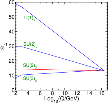
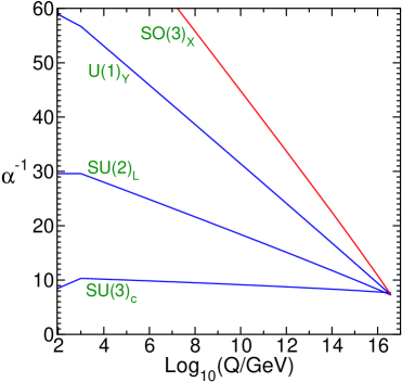
Figure 1: Renormalization group running of the inverses of the gauge couplings $\alpha_{1}$, $\alpha_{2}$, $\alpha_{3}$, and $\alpha_{X}$, for the minimal viable cases $G_{X}=SU(2)$ with $n_{S}=0$ (upper left), $G_{X}=SU(3)$ with $n_{S}=3$ (upper right) and $G_{X}=SO(3)$ with $n_{S}=0$ (lower left). The undiscovered MSSM particles and the new particles charged under $G_{X}$ are taken to have masses at a common threshold $M_{\rm thresh}=1$ TeV.

xxx

In the case of $SU(2)_{X}$ with $n_{S}=0$, the gauge coupling $g_{X}$ runs quite slowly, and is somewhat weaker than the QCD coupling at the TeV scale. In contrast, for the $SO(3)_{X}$ case with $n_{S}=0$, $g_{X}$ runs quickly to very small values in the infrared, due to a large positive beta function coefficient. For the minimal viable $SU(3)_{X}$ case with $n_{S}=3$, the $g_{X}$ beta function is even more negative than the QCD beta function, leading to a gauge coupling at the TeV scale that is larger, but still perturbative and not running very fast. For non-minimal models with $n_{S}$ larger than these values, the TeV-scale values of $\alpha_{X}$ are smaller, because the $g_{X}$ beta function is larger.

Below the masses of the quirks and their supersymmetric partners, the coupling $g_{X}$ has a negative beta function, and diverges at some scale $\Lambda$ when calculated at any particular loop order in a specified scheme. Given the $\overline{\rm MS}$ beta function for $\alpha_{X}=g_{X}^{2}/4\pi$ up to 4-loop order:

$$\beta_{\alpha_{X}}=Q\frac{d\alpha_{X}}{dQ}=-2\left(b_{0}\alpha_{X}^{2}+b_{1}\alpha_{X}^{3}+b_{2}\alpha_{X}^{4}+b_{3}\alpha_{X}^{5}+\ldots\right),$$ (2.18)

the scale $\Lambda$ can be defined, using any convenient $\alpha_{X}(Q_{0})$ with $Q_{0}\leq M_{\rm thresh}$ as input, by an expansion in inverse powers of $t\equiv\ln(Q_{0}^{2}/\Lambda^{2})$ Chetyrkin:1997un :

$$\alpha_{X}(Q_{0}) = \frac{1}{b_{0}t}\Bigl{(}1-[b_{1}\ln t]/b_{0}^{2}t+[b_{0}b_{2}+b_{1}^{2}(\ln^{2}t-\ln t-1)]/b_{0}^{4}t^{2}$$ (2.19)

$$+[b_{0}^{2}b_{3}-b_{1}^{3}(2\ln^{3}t-5\ln^{2}t-4\ln t+1)-6b_{0}b_{1}b_{2}\ln t]/2b_{0}^{6}t^{3}+\ldots\Bigr{)}.$$

It is common in rough estimates to only use the one-loop-order estimate $\alpha_{X}(Q_{0})=1/b_{0}t$, with $b_{0}=(11C_{A}-2T_{F})/12\pi$ where $(C_{A},T_{F})=(N,n)$ for $SU(N)_{X}$ and $(C_{A},T_{F})=(2,2n)$ for $SO(3)_{X}$, with $n$ denoting the number of the $n_{S}$ SM singlet fields that have masses below $Q_{0}$ and are treated as non-decoupled below $M_{\rm thresh}$. However, it turns out that including the higher loop effects (with coefficients $b_{1,2,3}$ found in refs. fourloop ) are quite important for obtaining a stable value of the $G_{X}$ confinement scale $\Lambda$. This is illustrated in Table 1, which shows the results obtained for $\Lambda^{(\ell)}_{\overline{\rm MS}}$ at various loop orders $\ell$, assuming again that the effective decoupling scale for particles charged under $G_{X}$ is $M_{\rm thresh}=1$ TeV.

$G_{X}$	$n_{S}$	$\alpha_{X}^{-1}$(1 TeV)	$\Lambda^{(1)}$	$\Lambda^{(2)}$	$\Lambda^{(3)}$	$\Lambda^{(4)}$
$SU(2)$	0	9.3	0.35 GeV	1.3 GeV	1.1 GeV	1.1 GeV
	1	14.4	4.4 MeV	19 MeV	17 MeV	17 MeV
	2	19.5	57 keV	280 keV	250 keV	250 keV
	3	24.5	0.76 keV	4.1 keV	3.7 keV	3.7 keV
	4	29.5	11 eV	60 eV	55 eV	55 eV
$SU(3)$	3	4.9	61 GeV	140 GeV	120 GeV	120 GeV
	4	9.9	3.5 GeV	11 GeV	9.3 GeV	9.5 GeV
	5	15.0	190 MeV	720 MeV	620 MeV	620 MeV
	6	20.1	10 MeV	44 MeV	38 MeV	38 MeV
	7	25.1	0.59 MeV	2.7 MeV	2.4 MeV	2.4 MeV
	8	30.2	32 keV	160 keV	140 keV	140 keV
	9	35.2	1.9 keV	9.7 keV	8.7 keV	8.8 keV
$SO(3)$	0	83	$1.3\!\times\!10^{-19}$ eV	$1.1\!\times\!10^{-18}$ eV	$1.0\!\times\!10^{-18}$ eV	$1.0\!\times\!10^{-18}$ eV
	1	103	$4.7\!\times\!10^{-27}$ eV	$4.4\!\times\!10^{-26}$ eV	$4.2\!\times\!10^{-26}$ eV	$4.2\!\times\!10^{-26}$ eV

Table 1: The $G_{X}$ confinement scale $\Lambda^{(\ell)}_{\overline{\rm MS}}$, computed at various loop orders $\ell$ by using eq. (2.19) keeping terms of order $1/t^{\ell}$. The new particles charged under $G_{X}$ are taken to have an effective average decoupling mass scale of $Q_{0}=M_{\rm thresh}=1$ TeV, with no SM singlet quirks with current masses $\mu_{S_{i}}$ smaller than $\Lambda$.

The point of carrying the calculation to 4-loop order is not because of the very slightly increased accuracy obtained (since there are threshold uncertainties here that are not known), but rather to demonstrate the stability of the results with respect to inclusion of higher-order terms. In fact, the 4-loop order results for $\Lambda$ hardly differ at all from the 3-loop order ones, and only at the 10% level from the 2-loop order ones. However, they are notably larger than the 1-loop order estimate, which is therefore judged to be deprecated as an estimate of the physical $G_{X}$ confinement scale.

Table 1 shows that the confinement scale $\Lambda$ for $SO(3)_{X}$ is very small in energy units. In terms of length, the confinement scale for the minimal model $n_{S}=0$ is of the order $10^{11}$ meters, very roughly of order the radius of the Earth’s orbit around the Sun. For $n_{S}=1$, the confinement length is of order 100 parsecs. Thus for all practical purposes, the quirks are actually free. Adding other SM singlets charged under $SO(3)_{X}$ will only decrease $\Lambda$, making the confinement length even larger.

For the minimal viable $SU(2)_{X}$ and $SU(3)_{X}$ models, the confinement energy scale is much larger. Increasing $n_{S}$ leads to smaller $\Lambda$, as indicated in Table 1. If $n$ of the $n_{S}$ SM singlets charged under $G_{X}$ have current masses $\mu_{S_{i}}$ less than $\Lambda$, the confinement scale will be decreased. This is illustrated in Table 2 for the extreme case that all $n=n_{S}$ of the new singlets are lighter than $\Lambda$.

$G_{X}$	$n_{S}=n$	$\alpha_{X}^{-1}$(1 TeV)	$\Lambda^{(4)}$
$SU(2)$	1	14.4	5.0 MeV
	2	19.5	6.3 keV
	3	24.5	1.3 eV
	4	29.5	$2.0\times 10^{-5}$ eV
$SU(3)$	3	4.9	68 GeV
	4	9.9	1.5 GeV
	5	15.0	13 MeV
	6	20.1	38 keV
	7	25.1	30 eV
	8	30.2	0.0030 eV
	9	35.2	$2.1\times 10^{-8}$ eV

Table 2: As in Table 1, but now taking all $n_{S}=n$ of the SM singlet fermions to have current masses much less than $\Lambda$, and showing only the 4-loop order result (which is nearly identical to the 3-loop order result in all cases).

Both Tables 1 and 2 take the effective average decoupling scale for the particles in the other new chiral supermultiplets (including both scalars and fermions) to be 1 TeV. More generally one can estimate:

$$\Lambda=\Lambda_{\rm tab}\left(\frac{M_{\rm thresh}}{\mbox{TeV}}\right)^{1-\Delta},\qquad\Delta=\frac{3C_{A}-5-n_{S}}{(11C_{A}-2n)/3},$$ (2.20)

where now $\Lambda_{\rm tab}$ is the value given in Table 1 for $n=0$, or Table 2 for $n=n_{S}$. Here, $M_{\rm thresh}$ is defined to be the effective average decoupling scale for the new supermultiplets, at which the threshold corrections to the gauge coupling $g_{X}$ are small. As seen in Figure 1, in the minimal viable models the $g_{X}$ coupling runs fairly slowly in the non-decoupled theory above $Q=M_{\rm thresh}$. This means that in the minimal model for $SU(2)_{X}$, $\Lambda\approx 0.001M_{\rm thresh}$, while for the minimal viable $SU(3)_{X}$ model with $n_{S}=3$, $\Lambda\approx 0.12M_{\rm thresh}$, if $n=0$.

If the Yukawa couplings $k,k^{\prime}$ are present, there is a potentially important constraint from precision electroweak observables. The new contributions to the Peskin-Takeuchi $S,T$ observables from the new fermions are:

$$\Delta T = \frac{Nv^{4}}{480\pi s_{W}^{2}M_{W}^{2}M_{F}^{2}}[13(\hat{k}^{4}+\hat{k}^{\prime 4})+2(\hat{k}^{3}\hat{k}^{\prime}+\hat{k}\hat{k}^{\prime 3})+18\hat{k}^{2}\hat{k}^{\prime 2}],$$ (2.21)

$$\Delta S = \frac{Nv^{2}}{30\pi M_{F}^{2}}[4\hat{k}^{2}+4\hat{k}^{\prime 2}-7\hat{k}\hat{k}^{\prime}].$$ (2.22)

where $\hat{k}=k\sin\beta$ and $\hat{k}^{\prime}=k^{\prime}\cos\beta$ and $v\approx 175$ GeV, and for illustration purposes I have chosen $\mu_{L}\approx\mu_{S}\gg m_{Z}$ and assumed that the corresponding scalars are much heavier. The values of these Yukawa couplings are governed by infrared quasi-fixed points. For example, if $k^{\prime}$ is negligible, then the beta functions for $k$ and the top Yukawa coupling are given at one-loop order by:

$$Q\frac{dy_{t}}{dQ} = \beta_{y_{t}}=\frac{y_{t}}{16\pi^{2}}\left[6y_{t}^{2}+y_{b}^{2}+Nk^{2}-\frac{16}{3}g_{3}^{2}-3g_{2}^{2}-\frac{13}{15}g_{1}^{2}\right],$$ (2.23)

$$Q\frac{dk}{dQ} = \beta_{k}=\frac{k}{16\pi^{2}}\left[(3+N)k^{2}+3y_{t}^{2}-4Cg_{X}^{2}-3g_{2}^{2}-\frac{3}{5}g_{1}^{2}\right],$$ (2.24)

where $N=2$, $3$, or $3$ and $C=3/4$, $4/3$, or $2$ for $G_{X}=SU(2)$, $SU(3)$, or $SO(3)$ respectively. The fixed points arise due to the balancing between the positive Yukawa and the negative gauge contributions PRH . Including two-loop effects, I find for the minimal viable models the infrared quasi-fixed-point values:

$$k_{\rm fixed}=\left\{\begin{array}[]{l}0.88\qquad[SU(2)_{X},n_{S}=0]\\[-9.0pt] 0.76\qquad[SO(3)_{X},n_{S}=0]\\[-9.0pt] 1.32\qquad[SU(3)_{X},n_{S}=3].\end{array}\right.$$ (2.28)

at $Q=1$ TeV. The resulting contributions to $S,T$ can be used to put a lower bound on $\mu_{L}$. Requiring the results to be within the current 95% CL ellipse from experimental results on $m_{t}$, $m_{W}$, and $Z$-peak observables using the same methodology as in Martin:2009bg , I estimate $\mu_{L}>210,225,380$ GeV for the $G_{X}=SU(2),SO(3),SU(3)$ fixed point cases respectively. However, $G_{X}$ confinement may play a significant role in modifying this estimate for $SU(3)$, because $\Lambda$ in that case is larger than $M_{Z}$. For smaller Yukawa couplings $k\ll k_{\rm fixed}$, there is no constraint as the vector-like particles decouple from precision electroweak observables.

III Soft SUSY-breaking masses and the sparticle spectrum

The presence of new vector-like supermultiplets has a profound effect on the spectrum of superpartner masses. They cause the $G_{\rm SM}$ gauge couplings to run to much larger values in the ultraviolet as they approach unification, resulting in bigger one-loop contributions to soft scalar squared masses from RG running, compared to the MSSM. The new supermultiplets also allow the $G_{X}$ gaugino masses to contribute indirectly to MSSM gaugino and sfermion masses, through two-loop order effects. In this section, the patterns of soft supersymmetry breaking masses will be considered for these models. For simplicity, the discussion will be mostly limited to the scenario in which a unified gaugino mass parameter $m_{1/2}$ is much larger than the scalar masses and other sources of supersymmetry breaking at the RG scale where the gauge couplings unify. This gaugino mass dominated limit is motivated as a solution to the supersymmetric flavor problem, since it automatically produces flavor-blind soft terms.

The modified running of the gaugino masses pushes them to be smaller near the TeV scale than they would be in the MSSM. Given an input unified gaugino mass $m_{1/2}$ at the unification scale, one finds for the running gaugino masses at $Q=1$ TeV:

$$(M_{1},\>M_{2},\>M_{3}) = m_{1/2}\times\left\{\begin{array}[]{ll}(0.41,\>0.77,\>2.28)&\mbox{[MSSM],}\\[-7.0pt] (0.21,\>0.39,\>1.16)&\mbox{[$SU(2)$, $n_{S}=0$],}\\[-7.0pt] (0.112,\>0.20,\>0.57)&\mbox{[$SO(3)$, $n_{S}=0$],}\\[-7.0pt] (0.080,\>0.135,\>0.40)&\mbox{[$SU(3)$, $n_{S}=3$].}\end{array}\right.$$ (3.5)

Thus, in the extended models, to obtain the same physical gaugino masses, one must start with larger $m_{1/2}$ than one would in the MSSM. Since $m_{1/2}$ is not directly observable, it is also interesting to consider the ratios of these gaugino masses. They are also affected, but more mildly (being due to 2-loop effects):

$$(M_{2}/M_{1},\>M_{3}/M_{2},\>M_{3}/M_{1}) = \left\{\begin{array}[]{ll}(1.87,\>2.96,\>5.53)&\mbox{[MSSM],}\\[-7.0pt] (1.85,\>2.95,\>5.44)&\mbox{[$SU(2)$, $n_{S}=0$],}\\[-7.0pt] (1.79,\>2.84,\>5.09)&\mbox{[$SO(3)$, $n_{S}=0$],}\\[-7.0pt] (1.73,\>2.85,\>4.95)&\mbox{[$SU(3)$, $n_{S}=3$],}\end{array}\right.$$ (3.10)

where again unification of gaugino masses at the gauge coupling unification scale is assumed. The effect of the additional fields is thus to somewhat compress the gaugino mass spectrum compared to the MSSM case, with the ratio of gluino to bino masses decreased by about 10 per cent for $G_{X}=SO(3)$ and $SU(3)$. To obtain the physical masses, one must also include mixing with Higgsinos and the pole mass corrections, which are particularly important for the gluino MV ; PBMZ ; MV2 .

In the extended models the squark and slepton masses are also relatively smaller (compared to $m_{1/2}$) at the TeV scale than in the MSSM. Taking a gaugino-mass dominated scenario (by assuming a vanishing common scalar squared mass $m_{0}^{2}=0$ at the unification scale), one finds for the first and second family squark and slepton masses at $Q=1$ TeV:

$$(m_{\widetilde{q}_{1}},\,m_{\widetilde{\bar{u}}_{1}},\,m_{\widetilde{\bar{d}}_{1}},\,m_{\tilde{\ell}_{1}},\,m_{\widetilde{\bar{e}}_{1}}) = m_{1/2}\!\times\!\left\{\begin{array}[]{ll}(2.15,\,2.08,\,2.07,\,0.67,\,0.37)&\mbox{[MSSM],}\\[-7.0pt] (1.61,\,1.55,\,1.54,\,0.57,\,0.33)&\mbox{[$SU(2)$, $n_{S}=0$],}\\[-7.0pt] (1.23,\,1.18,\,1.17,\,0.48,\,0.28)&\mbox{[$SO(3)$, $n_{S}=0$],}\\[-7.0pt] (1.06,\,1.02,\,1.01,\,0.43,\,0.26)\quad\!\!&\mbox{[$SU(3)$, $n_{S}=3$].}\end{array}\right.\phantom{x.x}$$ (3.15)

This shows that there is also a compression within the sfermion mass spectrum, as the ratio of the squarks to the slepton masses is decreased in the extended models compared to the MSSM in the $m_{0}^{2}=0$ limit, or more generally for any given value of $m_{0}$. This is because of the increased relative importance of the contribution to scalar masses from large renormalization scales where all of the gauge couplings and gaugino masses are larger.

Despite these compressions in the gaugino and sfermion sectors considered separately, the combined sparticle spectrum in the extended models is stretched rather than compressed compared to the MSSM. Comparing eqs. (3.5) and (3.15), one observes that in each of the extended models, the bino is much lighter than the lightest slepton, and so the lightest supersymmetric particle (LSP) will be a neutralino. This is in contrast to the well-known fact that the $m_{0}^{2}=0$ scenario in the MSSM problematically predicts a stau as the LSP. The supersymmetry-breaking flavor problem thus can be naturally solved by taking $m_{0}^{2}\ll m_{1/2}^{2}$ in the extended models without running into the difficulties found in the gaugino mass dominated MSSM.

Now consider the soft supersymmetry breaking masses for the new particles. Assuming gaugino mass unification, the $G_{X}$ gaugino is heavier than all of the MSSM gauginos in the minimal $G_{X}=SU(2)$ and $SU(3)$ cases, but it is lighter than the MSSM gauginos if $G_{X}=SO(3)$. In terms of the unified gaugino mass parameter $m_{1/2}$, one finds at $Q=1$ TeV:

$$M_{\widetilde{X}} = m_{1/2}\!\times\!\left\{\begin{array}[]{ll}1.30&\mbox{[$SU(2)$, $n_{S}=0$],}\\[-7.0pt] 0.051&\mbox{[$SO(3)$, $n_{S}=0$],}\\[-7.0pt] 0.65\quad\!\!&\mbox{[$SU(3)$, $n_{S}=3$].}\end{array}\right.$$ (3.19)

[Compare eq. (3.5).] The scalar members of the $D,\overline{D}$ and $L,\overline{L}$ multiplets get RG contributions to their soft masses from both $G_{\rm SM}$ and $G_{X}$ gaugino loops. Therefore, they are heavier than their MSSM counterparts with the same gauge quantum numbers. For the case where $m_{1/2}$ dominates, one finds approximately for the soft masses $m_{\widetilde{D}}=m_{\widetilde{\overline{D}}}$ and $m_{\widetilde{L}}=m_{\widetilde{\overline{L}}}$, again at $Q=1$ TeV:

$$(m_{\widetilde{D}},\>m_{\widetilde{L}}) = m_{1/2}\times\left\{\begin{array}[]{ll}(1.97,\>1.40)&\mbox{[$SU(2)$, $n_{S}=0$],}\\[-7.0pt] (1.22,\>0.65)&\mbox{[$SO(3)$, $n_{S}=0$],}\\[-7.0pt] (1.68,\>1.51)&\mbox{[$SU(3)$, $n_{S}=3$].}\end{array}\right.$$ (3.23)

Also, for the minimal $SU(3)$ case with $n_{S}=3$, one finds that $m_{\widetilde{S}}=m_{\widetilde{\overline{S}}}=1.48m_{1/2}$. This is only slightly lower than $m_{\tilde{D}}$ and $m_{\tilde{L}}$, because most of the RG contribution to these soft masses comes from $\widetilde{X}$ loops in this case, which are the same for all of the new scalars.

The qualitative features of the above results are illustrated in Figure 2. The soft masses for the gauginos, the first-family sfermions, and the new scalars are shown for $Q=1$ TeV.

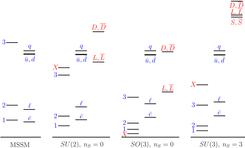
Figure 2: Comparison of the soft supersymmetry-breaking mass spectra following from a unified input gaugino mass $m_{1/2}$ that dominates at the unification scale, for the MSSM and the minimal models with $G_{X}=SU(2),SO(3),$ and $SU(3)$. The labels $1,2,3,X$ refer to running gauginos masses for $U(1)_{Y}$, $SU(2)_{L}$, $SU(3)_{c}$ and $G_{X}$, respectively. The labels $q,\bar{u},\bar{d},\ell,\bar{e}$ refer to MSSM first family squark and slepton soft masses, and the soft scalar masses for vectorlike supermultiplets are labeled with symbols $D$, $\overline{D}$, $L$, $\overline{L}$, and (for the $G_{X}=SU(3)$ case with $n_{S}=3$), $S,\overline{S}$. The value of $m_{1/2}$ is chosen so that the heaviest MSSM squark, $\tilde{q}$, has the same mass in each of the four cases.

For purposes of comparison, $m_{1/2}$ is chosen so that the heaviest MSSM squark, $\tilde{q}$, has the same mass in each of the four cases. The mass spectra in the extended models are readily distinguishable from the usual “mSUGRA” case parameterized by $m_{1/2},m_{0},A_{0}$. This is because obtaining such a large ratio of scalar masses to gaugino masses in mSUGRA, would require a large $m_{0}$, which in turn would lead to a much more compressed scalar mass spectrum. In contrast, the extended models are characterized by relatively heavy scalars which nevertheless maintain a significant hierarchy between squarks, left-handed sleptons, and right-handed sleptons, especially in the $G_{X}=SO(3)$ and $SU(3)$ cases.

In order to keep the discussion bounded, I will not give detailed results on the extended models with more singlets [$n_{S}>0$ for $G_{X}=SU(2)$ and $SO(3)$, and $n_{S}>3$ for $G_{X}=SU(3)]$. However, the following qualitative features are notable. First, at one loop order, the presence of additional $G_{\rm SM}$ singlets does not affect the RG running of MSSM-field soft terms, so the effects are rather mild on the gluino, wino, bino, and MSSM squark and slepton masses. Second, increasing $n_{S}$ will decrease both the $g_{X}$ gauge coupling and the $G_{X}$ gaugino soft mass at lower RG scales. Therefore, the $G_{X}$ gaugino mass $M_{\widetilde{X}}$ will be smaller compared to the MSSM gaugino masses $M_{1}$, $M_{2}$, and $M_{3}$ than in the cases shown in Figure 2. Also, the soft masses $m_{\widetilde{D}}=m_{\widetilde{\overline{D}}}$ and $m_{\widetilde{L}}=m_{\widetilde{\overline{L}}}$ will become relatively smaller, tending towards the MSSM squark and slepton masses $m_{\tilde{\bar{d}}}$ and $m_{\tilde{\ell}}$ respectively. The soft masses for $m_{\widetilde{S}}=m_{\widetilde{\overline{S}}}$ will also decrease for larger $n_{S}$, although they are always heavier than $M_{\tilde{X}}$, which decreases faster for larger $n_{S}$. For $n_{S}>0$, the Yukawa couplings $k,k^{\prime}$ can also come into play, decreasing the $\widetilde{L}$, $\widetilde{\overline{L}}$, $\widetilde{S}$, and $\widetilde{\overline{S}}$ soft supersymmetry breaking masses.

IV The $\mu$ parameter and the little hierarchy problem

The supersymmetric little hierarchy problem is a subjective but inspirationally important puzzle which questions the naturalness of viable model parameters. The essence of it is that once one applies constraints from the non-observation of a Higgs boson and of superpartners at both LEP2 and the Tevatron, the actual value of $m_{Z}$ might be considered surprisingly low for generic soft supersymmetry breaking parameters.

The largest loop correction to the $h^{0}$ mass in the MSSM is given by (in the decoupling limit $m^{2}_{A^{0}}\gg m^{2}_{h^{0}}$):

$$m^{2}_{h^{0}} = m_{Z}^{2}\cos^{2}(2\beta)+\frac{3}{4\pi^{2}}\sin^{2}\!\beta\>y_{t}^{2}\biggl{[}m_{t}^{2}\,{\rm ln}\left(m_{\tilde{t}_{1}}m_{\tilde{t}_{2}}/m_{t}^{2}\right)+c_{\tilde{t}}^{2}s_{\tilde{t}}^{2}(m_{\tilde{t}_{2}}^{2}-m_{\tilde{t}_{1}}^{2})\,{\rm ln}(m_{\tilde{t}_{2}}^{2}/m_{\tilde{t}_{1}}^{2})$$ (4.1)

$$+c_{\tilde{t}}^{4}s_{\tilde{t}}^{4}\Bigl{\{}(m_{\tilde{t}_{2}}^{2}-m_{\tilde{t}_{1}}^{2})^{2}-\frac{1}{2}(m_{\tilde{t}_{2}}^{4}-m_{\tilde{t}_{1}}^{4})\,{\rm ln}(m_{\tilde{t}_{2}}^{2}/m_{\tilde{t}_{1}}^{2})\Bigr{\}}/m_{t}^{2}\biggr{]},$$

where $m_{\tilde{t}_{1}}$ and $m_{\tilde{t}_{2}}$ are the top squark masses, and $c_{\tilde{t}}$ and $s_{\tilde{t}}$ are the cosine and sine of the top squark mixing angle $\theta_{\tilde{t}}$. Now in the models discussed in Babu:2004xg and this paper, adding in the effects of the Yukawa coupling $k$ one finds the further estimated correction in the case $\mu_{L}\approx\mu_{S}\approx M_{F}$ with heavier scalars with masses of order $M_{S}$ Babu:2004xg :

$$\Delta m_{h^{0}}^{2}=\frac{N}{4\pi^{2}}k^{4}v^{2}\sin^{4}\beta\left[f(x)+\frac{X_{k}^{2}}{M_{S}^{2}}(1-\frac{1}{3x})-\frac{X_{k}^{4}}{12M_{S}^{4}}\right].$$ (4.2)

Here $x=M_{S}^{2}/M_{F}^{2}$ is the ratio of the average new scalar and new fermion masses in the $L,\overline{L},S,\overline{S}$ sector, and $X_{k}=a_{k}/k-\mu\cot\beta$ is a mixing parameter for the scalars. The largest possible contributions come from the maximal (fixed-point) values of eq. (2.28). As was pointed out in ref. Babu:2004xg , for $G_{X}=SU(3)$ eq. (4.2) is enough to raise the Higgs mass by tens of GeV, depending on the details of the fermion and scalar masses in the new sector.

From the point of view of the supersymmetric little hierarchy problem, even raising the Higgs mass by a few GeV is potentially helpful. However, one must also consider the effect of the new sector on the scalar potential. The minimization of the Higgs potential in supersymmetry results in:

$$m_{Z}^{2}=-2(|\mu|^{2}+m^{2}_{H_{u}})-\frac{1}{v_{u}}\frac{\partial}{\partial v_{u}}\Delta V+{\cal O}(1/\tan^{2}\beta),$$ (4.3)

where $\Delta V$ is the radiative part of the effective potential, with $\tan\beta=v_{u}/v_{d}=\langle H_{u}^{0}\rangle/\langle H_{d}^{0}\rangle$ and $v_{u}$ treated as a real variable in the partial differentiation. In general, without further theoretical structure, $\mu$ and $m^{2}_{H_{u}}$ have no reason to be related, since $\mu$ is a supersymmetry-preserving parameter and $m^{2}_{H_{u}}$ is supersymmetry-breaking. In the MSSM with generic parameters, one finds that $-m^{2}_{H_{u}}$ tends to be much larger than $m_{Z}^{2}$, and eq. (4.3) seems to imply a percent-level fine-tuning of the difference between $|\mu|^{2}$ and $m_{H_{u}}^{2}$.

It is not possible to rigorously quantify fine tuning, since there can be no such thing as an objective measure on parameter space. Nevertheless, qualitative trends can be identified, and an obvious approach is to consider models with smaller predicted values of $-m_{H_{u}}^{2}$ at the weak scale to be more likely than those with very large $-m_{H_{u}}^{2}$, because then the fractional tuning required between it and $|\mu|^{2}$ will be less. This in turn means that smaller values of $|\mu|$ are more likely than very large values, since this is determined by eq. (4.3).

With this in mind, it is interesting to consider how the MSSM and its extensions, and variations of the most popular models of supersymmetry breaking, affect the weak-scale predictions for $-m^{2}_{H_{u}}$. For example, in the MSSM with $\tan\beta=10$ and $m_{t}=173.3$ GeV, one finds from RG running at $Q=1$ TeV in terms of the GUT-scale input parameters $m_{1/2}$, $A_{0}$ and $m_{0}$:

$$-m_{H_{u}}^{2}=1.65m_{1/2}^{2}-0.40m_{1/2}A_{0}+0.11A_{0}^{2}-0.022m^{2}_{0}.$$ (4.4)

This formula shows that $-m_{H_{u}}^{2}$, and therefore $|\mu|^{2}$, and therefore the level of fine-tuning required, increase with the gaugino squared masses. In extended models the gaugino masses at the unification scale have a varying relationship with the gaugino masses at the weak scale, which are more closely related to the physical masses, so it is useful to reformulate this in terms of the running gluino mass parameter $M_{3}$ also evaluated at $Q=1$ TeV:

$$-m_{H_{u}}^{2}=0.32M_{3}^{2}-0.18M_{3}A_{0}+0.11A_{0}^{2}-0.022m^{2}_{0},\qquad\mbox{[MSSM]}.$$ (4.5)

In fact, most of the dependence on the gaugino masses comes from the gluino mass Kane:1998im , so this formula is approximately valid even for moderate deviations from gaugino mass universality. One can note that for a gluino mass of order 500 GeV, and small $|A_{0}|$, $-m_{H_{u}}^{2}$ is only of order (280 GeV)², so that the tuning needed to get $m_{Z}^{2}$ in eq. (4.3) is of order 5%. The problem is that (although there is still considerable variation among models, particularly for large $|A_{0}|$) lower values of $M_{3}$ typically give a prediction for $m_{h^{0}}$ that is smaller than 114 GeV, and higher values of $M_{3}$ require even more delicate cancellation between $-m_{H_{u}}^{2}$ and $|\mu|^{2}$. The “focus point” region Chan:1997bi ; Feng:1999mn occurs due to the small negative coefficient of $m_{0}^{2}$ in eq. (4.5), which allows a cancellation between the $M_{3}^{2}$ and $m_{0}^{2}$ terms for very large $m_{0}^{2}$, leading to a small value of $-m_{H_{u}}^{2}$ and therefore small $|\mu|^{2}$. However, this also can be judged to be fine-tuned, as the large value of $m_{0}^{2}$ has to be finely adjusted, given a value of the ostensibly independent parameter $M_{3}$.

We can now compare with the situation for the models in the present paper. In the minimal $SU(2)_{X}$ model with $n_{S}=0$, one finds instead from the RG running:

$$-m_{H_{u}}^{2}=1.07M_{3}^{2}-0.44M_{3}A_{0}+0.12A_{0}^{2}-0.16m^{2}_{0},\qquad[SU(2)_{X},\>n_{S}=0].$$ (4.6)

again for $-m_{H_{u}}^{2}$ and $M_{3}$ evaluated at $Q=1$ TeV, assuming gaugino and scalar mass universality, $\tan\beta=10$ and $m_{t}=173.3$ GeV. (The coefficients change, but not very radically, for larger $n_{S}$.) The larger coefficient of $M_{3}^{2}$ indicates that this is naively even more fine-tuned than the MSSM. However, this effect is not without compensation; as Figure 2 shows, one does not need as large a gluino mass to get large squark masses, which in turn lead to large positive contributions to $m_{h^{0}}^{2}$ from eq. (4.1). Also, the larger negative coefficient of $m_{0}^{2}$ means that the analog of the MSSM focus point region occurs at much smaller values of $m_{0}^{2}$ in this extended model. Since there is no such thing as an objective quantitative measure of fine-tuning, I choose not to attempt to make a definitive statement beyond observing the competing factors just mentioned.

For $SO(3)_{X}$ with $n_{S}=0$, the analogous formula becomes:

$$-m_{H_{u}}^{2}=3.36M_{3}^{2}-0.91M_{3}A_{0}+0.13A_{0}^{2}-0.26m^{2}_{0},\qquad[SO(3)_{X},\>n_{S}=0].$$ (4.7)

Similarly, for the minimal viable $SU(3)_{X}$ model with $n_{S}=3$ and small Yukawa couplings $k,k^{\prime}\approx 0$, the analogous formula becomes:

$$-m_{H_{u}}^{2}=5.97M_{3}^{2}-1.28M_{3}A_{0}+0.13A_{0}^{2}-0.28m^{2}_{0},\qquad[SU(3)_{X},\>n_{S}=3].$$ (4.8)

In both of these cases, the situation again seems subjectively worse with respect to fine-tuning than the MSSM, due to the much larger coefficient of $M_{3}^{2}$. As shown in Figure 2, one does naturally get much larger squark masses for a given $M_{3}$, again leading to larger radiative corrections to $m_{h^{0}}^{2}$. However, with these large coefficients to $M_{3}$, the direct (but model dependent) constraints on the gluino mass from Tevatron come into play in a significant way. Again, there is a chance for more cancellation between the gaugino and scalar contributions due to the negative coefficient of $m_{0}^{2}$.

It is also interesting to consider the situation for $n_{S}\geq 1$ with large Yukawa couplings near the fixed points of eq. (2.28). For $SU(2)_{X}$ with $n_{S}=1$ and the fixed-point value $k=k_{\rm fixed}=0.88$ at $Q=1$ TeV, one finds:

$$-m_{H_{u}}^{2}=1.28M_{3}^{2}-0.15M_{3}A_{0}+0.04A_{0}^{2}+0.72m^{2}_{0},\qquad[SU(2)_{X},\>n_{S}=1,\>k=k_{\rm fixed}].$$ (4.9)

Here the coefficient of the gaugino mass squared is even larger than for $k=0$ [compare eq. (4.6)], and the coefficient of the scalar squared mass $m_{0}^{2}$ is large and positive, eliminating the possibility of cancellation to achieve a smaller $-m_{H_{u}}^{2}$. Similar results obtain for $SO(3)_{X}$ with $n_{S}=1$ and $k=k_{\rm fixed}=0.76$ at $Q=1$ TeV:

$$-m_{H_{u}}^{2}=3.46M_{3}^{2}-0.27M_{3}A_{0}+0.05A_{0}^{2}+0.89m^{2}_{0},\qquad[SO(3)_{X},\>n_{S}=1,\>k=k_{\rm fixed}],\phantom{xx}$$ (4.10)

and for $SU(3)_{X}$ with $n_{S}=3$ and one $k=k_{\rm fixed}=1.32$ at $Q=1$ TeV:

$$-m_{H_{u}}^{2}=17.0M_{3}^{2}-0.27M_{3}A_{0}+0.02A_{0}^{2}+0.71m^{2}_{0},\qquad[SU(3)_{X},\>n_{S}=3,\>k=k_{\rm fixed}].\phantom{xx}$$ (4.11)

Therefore, even though the fixed-point Yukawa coupling can give large positive contributions to $m_{h^{0}}^{2}$, there is a quite detrimental effect on the fine-tuning needed to obtain the observed $m_{Z}$ in models that have heavy enough gluinos (and charginos) to have evaded discovery at the Tevatron and LEP2. Similar effects have been noted before in the case of vector-like fermions without an additional gauge group in refs. Babu:2008ge , Martin:2009bg , Martin:2010dc .

Qualitatively, the model with $SU(2)_{X}$ and no new Yukawa coupling seems to be the least fine-tuned of the extended models. Adding new Yukawa couplings, despite increasing $m_{h^{0}}$, does not clearly alleviate the little hierarchy problem, and arguably make it much worse, especially in the cases of $SO(3)_{X}$ and $SU(3)_{X}$.

V Collider phenomenology of the quirks

In this section, I will consider some features of the phenomenology of the quirks in the models discussed above, following for the most part general ideas and results from refs. Kang:2008ea , Burdman:2008ek , Cheung:2008ke , and Harnik:2008ax . For simplicity, I will consider only the fermions from the $D,\overline{D}$, $L,\overline{L}$, multiplets, and not their scalar partners. This is because supersymmetry breaking effects provide for the scalars (“squirks”) and the $G_{X}$ gaugino to have much larger masses, making them less immediately relevant for collider searches. (Even if they had the same masses, squirks would have much smaller production cross-sections than fermionic quirks. The $G_{X}$ gauginos will not be produced directly in tree-level processes at colliders at all.) When produced, the squirks will decay promptly to quirks and MSSM gauginos. The $G_{X}$ gaugino can undergo a three-body decay to a quirk, antiquirk and MSSM gaugino, if kinematically allowed. In this section, I will use the same symbols for the fermions as for the chiral supermultiplets to which they belong.

I will also assume for simplicity, and motivated by the results of the previous section, that the mixing of the $G_{\rm SM}$ singlets $S,\overline{S}$ with the doublets $L,\overline{L}$ due to the Yukawa couplings $k,k^{\prime}$ is small in most of the following. This implies that $S,\overline{S}$ decouple from collider phenomenology. The charged $(L^{-},\overline{L}^{+})$ and neutral $(L^{0},\overline{L}^{0})$ fermions form two Dirac fermion-antifermion pairs, each with tree-level mass $\mu_{L}$. However, radiative corrections split the masses slightly, with $\Delta m\equiv m_{L^{-}}-m_{L^{0}}$ always positive. (If present, the Yukawa interactions $k,k^{\prime}$ that cause mixing with $S,\overline{S}$ would increase this splitting, so the lightest non-colored fermion is always neutral.) One finds $\Delta m>270$ MeV for $\mu_{L}>100$ GeV, with $\Delta m$ approaching 355 MeV asymptotically for large $\mu_{L}$ Thomas:1998wy . This means that the decays

$$\overline{L}^{+} \rightarrow \overline{L}^{0}\ell^{+}\nu_{\ell},\>\>\overline{L}^{0}\pi^{+},$$ (5.1)

$$L^{-} \rightarrow L^{0}\ell^{-}\overline{\nu}_{\ell},\>\>L^{0}\pi^{-},$$ (5.2)

(and decays to more pions or other SM hadrons if non-zero $k,k^{\prime}$ increase $\Delta m$) mediated by the $W$ boson are always kinematically allowed, and will occur with decay lengths of order centimeters Thomas:1998wy due to the small available kinematic phase space. Therefore, the lifetime of $\overline{L}^{+},L^{-}$ is large compared to other processes to be discussed below; in particular they will form quirk-antiquirk bound states and annihilate before they decay. In the simplest scenario (barring additional couplings to be described in the next paragraph), the neutral quirk Dirac fermions $L^{0},\overline{L}^{0}$ are completely stable, as are the colored quirks $D,\overline{D}$ with charges $\pm 1/3$. Note that none of the quirks can mix with the Standard Model fermions because of $G_{X}$ conservation, so the lightest quirk is always stable. Such stable fermions could present a challenge for the standard cosmology with a high reheat temperature but need not be a disaster Kang:2006yd ,Jacoby:2007nw ,Kang:2008ea .

If $n_{S}\geq 1$ and the pairs $L,\overline{L}$ and $S,\overline{S}$ have the opposite matter parity from each other, then the Yukawa couplings $k,k^{\prime}$ are forbidden, but the superpotential term

$$W=\lambda_{\ell}\overline{S}\hskip 1.084pt\overline{L}\hskip 0.3617pt\ell$$ (5.3)

is allowed, with $\ell$ an MSSM $SU(2)_{L}$ doublet lepton. This provides additional possible decay modes $\overline{L}^{+}\rightarrow S\tilde{\ell}_{L}^{+}$ and $L^{-}\rightarrow\overline{S}\tilde{\ell}^{-}_{L}$, if $|\mu_{L}|>|\mu_{S}|+m_{\tilde{\ell}_{L}}$ so that these decays are kinematically allowed, or alternatively with the sleptons off-shell. These decays are not automatically kinematically suppressed, and so could happen promptly before quirk-antiquirk annihilation occurs. The fermions $D$ and ${\overline{D}}$ may also have additional decay modes, if the possible superpotential terms

$$W=\lambda_{q}L\overline{D}q+\lambda_{\overline{d}}\overline{S}D\overline{d},$$ (5.4)

are present. The first of these terms is only allowed if $G_{X}$ is either $SU(2)$ or $SO(3)$, and if $L,\overline{L}$ have the opposite matter parity of $D,\overline{D}$ (if matter parity is conserved). It permits squark exchange to mediate the decays

$$D\rightarrow L^{0}\tilde{d}_{L},\quad L^{-}\tilde{u}_{L},$$ (5.5)

$$\overline{D}\rightarrow\overline{L}^{0}\tilde{d}_{L}^{*},\quad\overline{L}^{+}\tilde{u}_{L}^{*},$$ (5.6)

with the MSSM squarks possibly off-shell due to kinematics. The second term in eq. (5.4) is only allowed if $n_{S}\geq 1$ and $S,\overline{S}$ have the opposite matter parity of $D,\overline{D}$. Then MSSM squark exchange can mediate the decays

$$D\rightarrow S\tilde{d}_{R},\qquad\overline{D}\rightarrow\overline{S}\tilde{d}_{R}^{*},$$ (5.7)

again with the squarks possibly off-shell. Whether these decays can be important depends on the kinematics as well as the size of $\lambda_{\ell}$, $\lambda_{q}$, and $\lambda_{\overline{d}}$. For simplicity, they will be assumed to be absent or at least too small to make a difference below, except where noted otherwise.

The important direct pair-production processes for the new fermions are

$$pp \rightarrow D{\overline{D}},$$ (5.8)

$$pp \rightarrow Z^{(*)},\gamma^{(*)}\>\rightarrow\>\overline{L}^{+}L^{-},\>\,\overline{L}^{0}L^{0},$$ (5.9)

$$pp \rightarrow W^{+(*)}\>\rightarrow\>\overline{L}^{+}L^{0},$$ (5.10)

$$pp \rightarrow W^{-(*)}\>\rightarrow\>\overline{L}^{0}L^{-},$$ (5.11)

for the LHC, with the obvious substitution of $p\overline{p}$ for the Tevatron. Pair-produced quirks with masses much larger than $\Lambda$ will move apart from each other with typically semi-relativistic speeds, and as described in Kang:2008ea , will be connected by $G_{X}$ flux strings with tension $\sigma$. From the lattice, there is an estimate (see Table 7 and eq. (11) of Allton:2008ty ):

$$\sqrt{\sigma}=\Lambda_{\overline{\rm MS}}\times\biggl{\{}\begin{array}[]{l}1.73\quad SU(2)_{X},\\[-6.0pt] 1.86\quad SU(3)_{X},\end{array}\Biggr{.}$$ (5.14)

so that the maximum string length in a given hard scattering event with kinetic energy $\Delta E$ in the center-of-momentum frame is

$$L=\frac{\Delta E}{\sigma}\approx 6\,\mbox{mm}\>\left(\frac{\Delta E}{\mbox{100 GeV}}\right)\left(\frac{\mbox{keV}}{\Lambda_{\overline{\rm MS}}}\right)^{2}.$$ (5.15)

Therefore, the lengths of such strings, although much larger than $\Lambda^{-1}$, will typically be less than 1 mm for $\Lambda$ greater than a few keV. From Table 1, one finds that the quirky flux strings will be microscopic for $SU(2)_{X}$ with $n_{S}\leq 3$ and for $SU(3)_{X}$ with $n_{S}\leq 9$, assuming that $g_{X}$ is unified with the SM gauge couplings and all singlets charged under $SU(N)_{X}$ are heavier than $\Lambda$.

For the case of $G_{X}=SO(3)$, the situation is quite different, because from Table 1 the confinement distance scale $\Lambda^{-1}$ is literally astronomical, at least of order the Earth’s orbit around the Sun even in the minimal model. The quirks in this case are essentially free particles with multiplicity 3 times larger than expected from their SM quantum numbers. Note that even if one rejected the unification of $g_{X}$ with the SM gauge couplings in this model to arrive at a much larger $\Lambda$, the fact that the supermultiplets are in the adjoint representation of the Lie algebra means that they would not form stable flux tubes of the type discussed in Kang:2008ea when pair-produced, even if any $S,\overline{S}$ fields are heavier than $\Lambda$ (so $n=0$). Instead, pair-produced particles charged under $SO(3)_{X}$ would each bind to a gauge boson to form two stable $G_{X}$-singlet states with size of order $\Lambda^{-1}$, allowing the flux tube to break. Although the new fermions behave like free stable particles when pair-produced at colliders, the fact that they will come in three-fold exactly degenerate multiplets will in principle allow a determination of their nature from their production cross-sections. In the simplest case, $D,\overline{D}$ and $\overline{L}^{0},L^{0}$ will be absolutely stable, with $\overline{L}^{+},L^{-}$ having decays to $\overline{L}^{0},L^{0}$ via soft pion or lepton emission as discussed above. The $\overline{L}^{0},L^{0}$ are only weakly interacting and thus invisible, but known collider search strategies Abe:1989es for stable strongly interacting particles apply for $D,\overline{D}$. However, as noted above, $D,\overline{D}$ may be able to promptly decay according to eqs. (5.5)-(5.7), depending on both kinematics and the allowed superpotential terms. If so, then the signatures will always contain $E_{T}^{\rm miss}$, and will resemble those for ordinary MSSM squarks.

For the remainder of this section, consider the cases of $SU(2)_{X}$ and $SU(3)_{X}$, with the $G_{X}$ confinement scale less than the masses of the quirks that have SM gauge interactions, and stable microscopic flux strings joining the quirk-antiquirk pairs. The quirk-antiquirk pair will then form an exotic bound state with invariant mass given approximately by the total center-of-momentum energy of the hard partonic scattering that produced them. This quirk-antiquirk string state can lose energy either by $G_{X}$-glueball emission, by radiation of many soft photons, or in the case of the $D\overline{D}$ state by radiation of numerous soft pions, a “hadronic fireball” Kang:2008ea . The large multiplicity of soft pions or photons may be detectable as anomalous “underlying events” Kang:2008ea ; Harnik:2008ax that accompany the hard scattering production, and may be used as an additional tag to dramatically reduce backgrounds.

If the quirk and antiquirk lose most of their initial relative kinetic energy before annihilating, they will briefly form a “quirkonium” bound state which then decays to two or three hard partons with invariant mass peaked at twice the mass of the quirk Kang:2008ea . Alternatively, however, the neutral and colorless quirk and antiquirk states might Kang:2008ea have a prompt annihilation before they can lose enough energy to form a low-lying quirkonium state. In that case, the final states will have a broad distribution of annihilation products, which will therefore be much harder to discern above hadron collider backgrounds. It is difficult to estimate in advance what proportion of the events will fall into these two categories, due to the non-perturbative nature of the energy loss mechanisms, which do not have direct analogs in experimentally known hadronic physics.

For the weakly interacting quirks, and for the strongly interacting quirks if $\Lambda>\Lambda_{\rm QCD}$, one might suspect the non-perturbative interactions by which the quirk-antiquirk string state loses energy to be dominated by $G_{X}$-glueball emission. However, this is quite uncertain, and can be suppressed or even eliminated by kinematics if $\Lambda\gg\Lambda_{\rm QCD}$. The masses of the $G_{X}$ glueballs have been estimated by lattice computations Teper:1998kw -Lucini:2001ej , Allton:2008ty , with the results for the lightest two glueball states with $J^{PC}=0^{++}$ and $2^{++}$:

$$m_{0^{++}} = 6.7\Lambda_{\overline{\rm MS}},$$ (5.16)

$$m_{2^{++}} = 9.6\Lambda_{\overline{\rm MS}}.$$ (5.17)

There are other heavier glueball states $0^{++*}$, $3^{++}$, $0^{-+}$, $2^{-+}$, $0^{-+*}$, $2^{-+*}$, and, for $SU(3)_{X}$ only there are also states with odd $C$, $1^{+-}$, $3^{+-}$, $2^{+-}$, $0^{+-}$, $1^{--}$, $2^{--}$ $3^{--}$, with masses ranging up to about $3m_{0^{++}}$. As can be seen from Tables 1 and 2, in the case of $SU(3)_{X}$ these glueballs should have masses in the hundreds of GeV range for the minimal case of $n_{S}=3$ and so could be comparable in mass or even heavier than the lighter quirks, and should be in the tens of GeV range for $n_{S}=4$. This would prohibit energy loss of the quirk-antiquirk flux string states into $G_{X}$-glueballs. For the other cases listed in Table 1, decays of the flux strings to $G_{X}$-glueballs should be allowed, but perhaps kinematically suppressed, leading to considerable uncertainty in the number of $G_{X}$-glueball states emitted and the likelihood of the quirk-antiquirk string state to lose most of its energy before annihilating. It is also possible that a few $G_{X}$-glueballs will be produced in the original hard scattering production.

If produced, the detection of $G_{X}$-glueballs is problematic. Their decay widths can be estimated for $SU(3)_{X}$ using eqs. (17), (23) and (30) of ref. Juknevich:2009ji (see also ref. Juknevich:2009gg ) with matrix elements from eqs. (38) and (62) of ref. Chen:2005mg :

$$\Gamma(0^{++}\rightarrow gg) = 360\,\alpha_{S}^{2}{\Lambda^{9}}/{\mu_{D}^{8}},$$ (5.18)

$$\Gamma(2^{++}\rightarrow gg) = 0.12\,\alpha_{S}^{2}{\Lambda^{9}}/{\mu_{D}^{8}},$$ (5.19)

$$\Gamma(0^{-+}\rightarrow gg) = 24\,\alpha_{S}^{2}{\Lambda^{9}}/{\mu_{D}^{8}}.$$ (5.20)

The results for $SU(2)_{X}$ should be comparable and slightly smaller. This leads to proper decay lengths for $G_{X}$-glueballs of order

$$c\tau=\left(\frac{0.2}{\alpha_{S}}\right)^{2}\left(\frac{\mu_{D}}{\mbox{100 GeV}}\right)^{8}\left(\frac{\mbox{GeV}}{\Lambda}\right)^{9}\times\left\{\begin{array}[]{l}0.14\>{\rm meters}\quad\mbox{(for $0^{++}$)},\\[-9.0pt] 400\>{\rm meters}\quad\mbox{(for $2^{++}$)},\\[-9.0pt] 2\>{\rm meters}\quad\mbox{(for $0^{-+}$)}.\end{array}\right.$$ (5.24)

If $\Lambda\approx 1$ GeV as expected for the minimal $SU(2)_{X}$ model, a sizable fraction of the $0^{++}$ decays might occur within the detector, but only if $\mu_{D}$ is less than roughly 150 GeV, which may be ruled out already by Tevatron data (see below). For larger $\mu_{D}$ or smaller $\Lambda$, the decays of the $G_{X}$-glueball will occur outside of the detector and will be invisible. For much larger $\Lambda$ as occurs in the $SU(3)_{X}$ model with $n_{S}=3$ or 4, the decays may occur within the detector for any $\mu_{D}$, but then the production of $G_{X}$ glueballs in the flux-tube energy loss processes is likely irrelevant anyway due to kinematic suppression or prohibition. Even if the $G_{X}$ glueballs are produced and decay promptly, the main decay is likely to a pair of gluons, and the resulting dijet mass peak signal from these decays will have to compete with a huge background from QCD. To have a significant branching fraction to $\gamma\gamma$, which has much smaller backgrounds, one can take $\mu_{L}<\mu_{D}$, with a leading-order estimate Juknevich:2009ji ; Juknevich:2009gg :

$$\frac{{\rm BR}(0^{++}\rightarrow\gamma\gamma)}{{\rm BR}(0^{++}\rightarrow gg)}=\frac{8\alpha^{2}}{9\alpha_{S}^{2}}\left(\frac{1}{4}+\frac{3\mu_{D}^{4}}{4\mu_{L}^{4}}\right)^{2}.$$ (5.25)

For example, with $\alpha_{S}\approx 0.2$, this ratio is of order 0.001 for $\mu_{L}=\mu_{D}$, but it rises to about 0.18 if $\mu_{L}/\mu_{D}=0.5$, and is greater than 1 if $\mu_{L}/\mu_{D}$ is less than $0.4$. The non-perturbative nature of the $G_{X}$ glueball production mechanisms means that the diphoton signal strengths, if any, are extremely difficult to estimate even roughly, but to have even a hope of observation would seem to require $\mu_{L}<\mu_{D}$ and $\Lambda$ of order a few GeV (not too small for $c\tau$ to be large, but not too large for $G_{X}$-glueball production to be kinematically suppressed). Nevertheless, given the uncertainties involved, this possibility highlights the general importance of searching for narrow diphoton peaks at large invariant masses at the LHC; this type of signal could also arise not only for the classic diphoton signal for a low-mass Higgs scalar boson, but also for stoponium stoponium1 ; stoponium2 or for Kaluza-Klein gravitons in theories with low-scale gravity Lemaire:2006kf .

Probably the most optimistic scenario for detecting the quirks occurs in the case that $D\overline{D}$ are strongly produced at a hadron collider and manage to lose most of their initial relative kinetic energy stored in the $G_{X}$ flux tube by radiating soft pions and/or $G_{X}$ glueballs, arriving at a low-lying quirkonium state with mass $\approx 2\mu_{D}$ before finally annihilating in a color-singlet $S$-wave ${}^{2S+1}L_{J}={}^{1}S_{0}$ ($\eta$) or ${}^{3}S_{1}$ ($\psi$) state. The most promising channel for detecting the quirkonium peak is $\mu^{+}\mu^{-}$. The relevant annihilation decay widths for a ${}^{3}S_{1}$ state can be inferred from refs. Barger:1987xg and Cheung:2008ke :

$$\Gamma(\psi\rightarrow f\overline{f})=4\alpha^{2}e_{D}^{2}N_{c}^{f}\beta_{f}\biggl{[}(1+2R_{f})\Bigl{(}e_{f}-\frac{g_{f}^{V}}{c_{W}^{2}(1-R_{Z})}\Bigr{)}^{2}+\Bigl{(}\frac{\beta_{f}g_{f}^{A}}{c_{W}^{2}(1-R_{Z})}\Bigr{)}^{2}\biggr{]}\Gamma_{0},\phantom{xxxxx}$$ (5.26)

$$\Gamma(\psi\rightarrow W^{+}W^{-})=\frac{\alpha^{2}e_{D}^{2}\beta_{W}^{3}}{4c_{W}^{4}}\frac{1+20R_{W}+12R_{W}^{2}}{(1-R_{Z})^{2}}\Gamma_{0}$$ (5.27)

$$\Gamma(\psi\rightarrow ggg)=\frac{40\alpha_{S}^{3}}{81\pi}(\pi^{2}-9)\Gamma_{0}$$ (5.28)

$$\Gamma(\psi\rightarrow XXX)=\frac{\alpha_{X}^{3}}{3\pi}\frac{(N^{2}-1)(N^{2}-4)}{N^{3}}(\pi^{2}-9)\Gamma_{0}$$ (5.29)

where $e_{f}=(2/3,-1/3,-1,0)$ and $N_{c}^{f}=(3,3,1,1)$ and $g_{f}^{A}=(1/4,-1/4,-1/4,1/4)$ for $f=(u,d,e,\nu)$ respectively, and $g_{f}^{V}=g_{f}^{A}-e_{f}s_{W}^{2}$, and $s_{W}$ and $c_{W}$ are the sine and cosine of the weak mixing angle, and $e_{D}=-1/3$, and $R_{i}=m_{i}^{2}/M^{2}$, where $M\approx 2\mu_{D}$ is the quirkonium mass, and $\beta_{i}=\sqrt{1-4R_{i}^{2}}$, and $\Gamma_{0}$ is a common normalization proportional to the square of the wavefunction at the origin. The $G_{X}$ gluon is represented by $X$. Note that final states $gg$, $ZZ$, $Z\gamma$, $\gamma\gamma$ and $XX$ do not occur in $\psi$ decays. The final states $Zgg$, $\gamma XX$, $ZXX$ do occur, but with branching ratios that turn out to be very small. For $N=2$, the decay to three $SU(2)_{X}$ gauge bosons vanishes due to the $N^{2}-4$ factor, and for $SU(3)_{X}$ with $N=3$ the $XXX$ decay will be kinematically forbidden or at least highly suppressed by the large masses of the $G_{X}$ glueballs that would have to be the final result of $G_{X}$-hadronization. Therefore final states involving $G_{X}$ glueballs should not play a significant role in quirkonium decays.

For ${}^{1}S_{0}$ states, the dominant decay is to $gg$ or $XX$, and $f\overline{f}$ does not occur at all at leading order. If we assume that the spin state is randomized by the non-perturbative processes that lose the initial relative kinetic energy, so that $\psi$ and $\eta$ states are populated in the ratio of 3 to 1, then the branching ratio of quirkonium to leptons should be given by 3/4 of the branching ratio indicated by eqs. (5.26)-(5.28). Numerically this yields BR$(D\overline{D}\rightarrow\mu^{+}\mu^{-})=0.093$ very nearly independent of the mass. It should be noted that this branching ratio does not apply to prompt annihilation of the quirks before they have settled into a color- and $G_{X}$-singlet quirkonium state; that branching ratio will be much smaller, and will not lead to a sharp dimuon peak, and so leads to a more pessimistic case.

In the most optimistic case that most of the $D\overline{D}$ states annihilate after losing most of their excess energy, there are good prospects for detection at hadron colliders, because the signal production is strong and peaked in invariant mass, while the dominant background is electroweak (Drell-Yan) and diffuse. The total production cross section at the Tevatron and at various LHC energies is shown in Figure 3. The CDF collaboration has published Aaltonen:2008ah a limit on cross-section times branching ratio for new states that decay to $\mu^{+}\mu^{-}$, based on 2.3 fb^-1 of $p\overline{p}$ collisions at the Tevatron. Comparing the relevant spin-0 limit from Figure 3 in Aaltonen:2008ah to the results shown in Figure 3 of the present paper and using the estimate BR$(\mu^{+}\mu^{-})=0.093$ from above, I obtain the lower mass bound $\mu_{D}>375$ GeV in this optimistic case.

At the LHC, the invariant mass resolution for high-mass dimuons should be of the order of 5% Belotelov:2006bb for the CMS detector. Therefore, as a rough estimate of the discovery reach, I consider a mass window from $0.9M$ to $1.1M$ where $M\approx 2\mu_{D}$ is the quirkonium mass, and require that $S/\sqrt{B}$ exceeds 5 in that window, where $S$ is the number of signal events (which is also required to exceed 10) and $B$ is the expected number of Drell-Yan background events. The Drell-Yan background cross-section is shown in Figure 4.

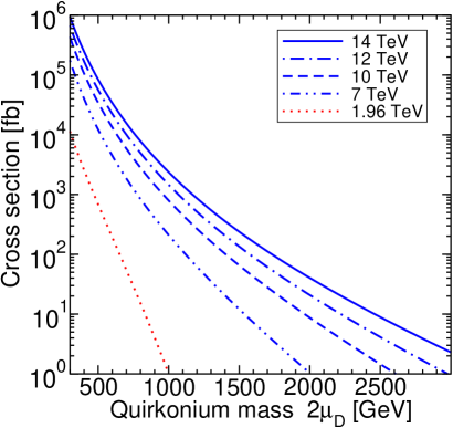
Figure 3: The production cross-section for $D\overline{D}$ in $pp$ collisions at $\sqrt{s}=14$, 12, 10, and 7 TeV, and in $p\overline{p}$ collisions at $\sqrt{s}=1.96$ TeV, obtained at leading order using CTEQ5LO CTEQ5 parton distribution functions (PDFs) with $Q=\mu_{D}$.

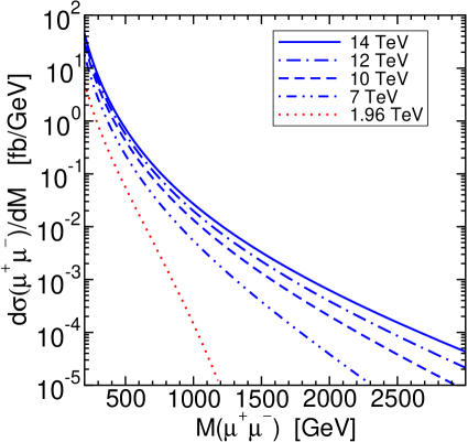
Figure 4: The leading-order differential production cross-section for the $\mu^{+}\mu^{-}$ background, through $\gamma^{*}$ and $Z^{*}$-mediated (Drell-Yan) processes in $pp$ collisions at $\sqrt{s}=14$, 12, 10, and 7 TeV, and in $p\overline{p}$ collisions at $\sqrt{s}=1.96$ TeV, as a function of the invariant mass of the $\mu^{+}\mu^{-}$ pair. CTEQ5LO CTEQ5 PDFs were used with $Q=\sqrt{\hat{s}}$.

Trigger and detector efficiencies are not included, but these are expected to be very high for high-mass dimuon events, and the QCD $K$-factor for the signal is not included. Dimuon backgrounds from sources other than Drell-Yan can be suppressed by requiring no extra hard jets or missing energy. In the following, I will again assume a spin-averaged BR$(\mu^{+}\mu^{-})=0.093$ for the signal. There is also a potential confirming signal from annihilation to $e^{+}e^{-}$, with an invariant mass peak that is similar but wider and smaller due to detector resolution and efficiency effects.

For a 1 fb^-1 LHC run at $\sqrt{s}=7$ TeV, the signal cross-section in Figure 3 yields 20 expected dimuon events for $\mu_{D}=500$ GeV, and as shown in Figure 4 there is about 1 background event expected in the corresponding mass window $M(\mu^{+}\mu^{-})=1000\pm 100$ GeV. Requiring 10 signal events, the discovery reach is up to about $\mu_{D}=550$ GeV.

For LHC $pp$ collisions at $\sqrt{s}=14$ TeV, the signal cross-section times dimuon branching ratio for $\mu_{D}=800$ GeV is 15 fb, with a background level in the mass window $M(\mu^{+}\mu^{-})=1600\pm 160$ GeV of 0.8 fb. Therefore, discovery may be possible in this case with 1 fb^-1. The mass reach is essentially determined by the number of signal events, since the background levels in the high-mass windows are small. In the same way, with 10 fb^-1, I estimate the 10-event discovery reach to be up to $\mu_{D}=1200$ GeV, and for 100 fb^-1 up to about $\mu_{D}$ = 1600 GeV.

In a more pessimistic scenario, the quirk and antiquirk may usually annihilate before they can settle into a low-lying color-singlet quirkonium state. The branching ratio to dileptons will be severely reduced in that case because there are color octet as well as color singlet decay states available, and the remaining dimuons will be distributed over larger invariant masses. If one supposes that only 10% of the $D\overline{D}$ pairs that are produced will settle into a low-lying color-singlet quirkonium state before annihilation, and uses only the dimuon events from this quirkonium peak, then the signal cross-section before BR$(\mu^{+}\mu^{-})$ is effectively ten times smaller than shown in Figure 3. The limit from comparing to the CDF bound on cross-section times branching ratio (Figure 3 in Aaltonen:2008ah , based on 2.3 fb^-1) results in $\mu_{D}>180$ GeV. I estimate that the expected reach from a 1 fb^-1 LHC run at $\sqrt{s}=7$ TeV in this more pessimistic case is roughly $\mu_{D}=350$ GeV, for which about 17 dimuon signal events and 6 background events would be expected in a mass window $M(\mu^{+}\mu^{-})=700\pm 70$ GeV. For LHC runs at $\sqrt{s}=14$ TeV with (1, 10, 100) fb^-1, I similarly estimate that the discovery reach for $D\overline{D}$ that annihilate at least 10% of the time from color-singlet $S$-wave quirkonium would extend to about $\mu_{D}=(500,800,1100)$ GeV.

In the case of the non-colored quirks $\overline{L}^{+},L^{-},\overline{L}^{0},L^{0}$, the production rates are electroweak, and the energy loss rate for the quirk-antiquirk bound by the flux string is much lower Kang:2008ea . The most promising signal may come from the production of the quirk-antiquirk states with a net $\pm 1$ charge, as in eqs. (5.10) and (5.11), because charge conservation then prohibits the subsequent prompt annihilation to invisible $G_{X}$ glueballs that may occur in the case of neutral bound states. The analogous case for fractionally charged squirks in “folded supersymmetry” was proposed and studied in Burdman:2008ek . The excess energy from the hard production will be radiated away in the form of $G_{X}$ glueballs or soft photons, hopefully allowing the quirk and antiquirk to finally annihilate when nearly at rest in a charged quirkonium bound state. The annihilation is strongest in an $S$-wave state. I will again assume that spins are randomized by the energy loss process, so that ${}^{3}S_{1}$ and ${}^{1}S_{0}$ states are populated in the ratio of 3 to 1. The branching ratios for such states have been computed in ref. Cheung:2008ke , and are shown in Figure 5 for the present case of constituent quirks with charges $\pm 1$ and $0$.

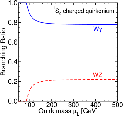
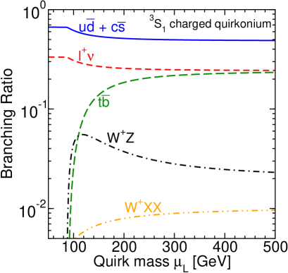
Figure 5: Branching ratios for charged quirkonium (a low-lying $\overline{L}^{+}L^{0}$ or $\overline{L}^{0}L^{-}$ bound state) in a ${}^{1}S_{0}$ (left panel) or a ${}^{3}S_{1}$ (right panel) state.

The ${}^{1}S_{0}$ state decays predominantly into $W\gamma$, with an invariant mass of nearly $2\mu_{L}$, and therefore a hard photon. (A somewhat smaller branching ratio to $W\gamma$ was obtained in ref. Cheung:2008ke for a case with fractionally charged constituent quirks.) This state may therefore be searched for in the $\ell^{\pm}\gamma+E_{T}^{\rm miss}$ channel at hadron colliders, as suggested in the similar squirk case of ref. Burdman:2008ek .

The combined production cross-sections at the Tevatron and at various possible LHC energies for the charged quirk-antiquirk combination are shown in Figure 6. These cross-sections are about an order of magnitude larger than for fractionally-charged scalar quirks (as studied in ref. Burdman:2008ek ) of the same mass.

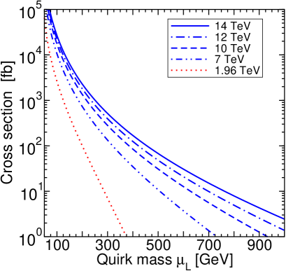
Figure 6: Combined leading-order production cross-section for $\overline{L}^{+}L^{0}$ and $\overline{L}^{0}L^{-}$ in $pp$ collisions at the LHC for $\sqrt{s}=14$, 12, 10, and 7 TeV, and in $p\overline{p}$ collisions at the Tevatron with $\sqrt{s}=1.96$ TeV. CTEQ5LO CTEQ5 PDFs were used with $Q=\mu_{L}$.

Partly counteracting this, one might expect that only about 1/4 of fermionic quirk-antiquirk production will end up in a ${}^{1}S_{0}$ state that can annihilate to $W\gamma$, rather than a ${}^{3}S_{1}$ state that decays mostly to jets or a single lepton plus neutrino. Thus, the effective branching ratio of charged quirkonium should be about $0.2$ for $W\gamma$, a factor of 3-4 smaller than used in Burdman:2008ek . The net effect is that the total production cross-section times branching ratio for $W\gamma$ should be a factor of 2-3 times larger, for a given quirkonium mass, than in the study of ref. Burdman:2008ek .

The largest background is from Standard Model $W\gamma$ production, which features a rapidly falling tail at high photon $p_{T}$. In contrast, the signal from ${}^{1}S_{0}$ quirkonium decaying to $W\gamma$ should have a photon $p_{T}$ distribution that is approximately flat, with an endpoint near $\mu_{L}-m_{W}^{2}/4\mu_{L}$ in the idealized case that the transverse kick to the quirkonium is small. The relevant photon $p_{T}$ distribution has been studied at Tevatron by both CDF CDFWgamma and D$\emptyset$ DzeroWgamma , where it was found that the data is described well by the SM $W\gamma$ and other subdominant backgrounds including $Wj$ with the jet faking a photon and $Z\gamma$ with one lepton from the $Z$ missed. At hadron colliders, a $W\gamma$ mass peak can in principle be reconstructed if one assumes that the observed $E_{T}^{\rm miss}$ in the event is due to the neutrino from the leptonic $W$ decay, but this is subject to the considerable uncertainty in how much missing energy is actually due to missing $G_{X}$-glueballs radiated from the initial state, as well as from the underlying event, additional jets, or from mismeasurement. However, the discovery potential may be greatly enhanced because one can also look for a large number of soft photons radiated as the quirk-antiquirk flux string loses energy, forming an anomalous “underlying event” with distinctive character. The resulting complications are beyond the scope of the present paper, but have been discussed in the analogous case of fractionally charged colorless squirks in Burdman:2008ek ; Harnik:2008ax . The search for $W\gamma$ candidates a with large photon $p_{T}$ and a possible peak in invariant mass or transverse mass, in combination with an anomalous underlying event used as a background-reducing tag, may well be the best hope to detect the quirks in these models.

VI Conclusions

Extensions of minimal supersymmetry with an extra non-Abelian gauge group and quirk supermultiplets maintain two of the hallmark successes of the MSSM: compatibility with perturbative gauge coupling unification and with constraints on precision electroweak observables. Natural mechanisms can put the quirk fermion masses at the TeV scale or below. It follows that requiring the unified gauge couplings to be perturbative, so that low-scale predictivity is not lost and the apparent unification of gauge couplings is not just an accident, the gauge group under which the new vector-like particles transform in the fundamental representation must be either $SU(2)$, $SU(3)$, or $SO(3)$. The presence of a new non-Abelian gauge group has a dramatic effect on the superpartner mass spectrum, and allows the soft supersymmetry breaking parameters to be dominated by the gaugino masses at the unification scale, while still having a neutralino LSP.

In the $SO(3)$ case, the confinement length scale is so large as to make the new particles essentially free in collider experiments. In contrast, in the minimal versions of the $SU(2)$ and $SU(3)$ cases, the quirk-antiquirk bound states produced at colliders will be microscopic. If a significant fraction of the colored quirk-antiquirk pairs produced at hadron colliders will lose most of their excess energy before annihilating as quirkonium, then there is significant reach in the dilepton mass peak channel. Even if this fraction is only 10%, Tevatron data that has already been analyzed should allow a limit of $180$ GeV for the quirk mass to be set from the search for a $\mu^{+}\mu^{-}$ resonance. In the optimistic idealized case that all of the quirk-antiquirk pairs annihilate from quirkonium, this limit should be about 375 GeV. In a 1 fb^-1 LHC run at $\sqrt{s}=7$ TeV, the discovery reach could be as high as 550 GeV, and should extend well above 1 TeV with 100 fb^-1 at $\sqrt{s}=14$ TeV. The color singlet quirks in these models can also be searched for as quirkonium $W\gamma$ resonances. In all cases, the quirkonium peak can be accompanied by an anomalous underlying event consisting of many soft pions or photons, which can significantly aid in making a discovery Kang:2008ea ; Harnik:2008ax . If low-energy supersymmetry is realized in nature, then it will be important to test the possibility that it is not minimal by searching for these events.

Acknowledgments: I am grateful to Ricky Fok, Roni Harnik, José Juknevich, and Graham Kribs for helpful communications. This work was supported in part by the National Science Foundation grant number PHY-0757325.

References

- (1) M.E. Peskin and T. Takeuchi, Phys. Rev. Lett. 65, 964 (1990), Phys. Rev. D 46, 381 (1992).
- (2) M. Golden and L. Randall, Nucl. Phys. B 361, 3 (1991).
- (3) B. Holdom and J. Terning, Phys. Lett. B 247, 88 (1990).
- (4) W.J. Marciano and J.L. Rosner, Phys. Rev. Lett. 65, 2963 (1990) [Erratum-ibid. 68, 898 (1992)].
- (5) D.C. Kennedy and P. Langacker, Phys. Rev. Lett. 65, 2967 (1990) [Erratum-ibid. 66, 395 (1991)]. Phys. Rev. D 44, 1591 (1991).
- (6) G. Altarelli and R. Barbieri, Phys. Lett. B 253, 161 (1991). G. Altarelli, R. Barbieri and S. Jadach, Nucl. Phys. B 369, 3 (1992) [Erratum-ibid. B 376, 444 (1992)].
- (7) For a review, S.P. Martin, “A supersymmetry primer,” [hep-ph/9709356] (version 5, December 2008).
- (8) K.S. Babu, I. Gogoladze and C. Kolda, “Perturbative unification and Higgs boson mass bounds,” [hep-ph/0410085].
- (9) T. Moroi and Y. Okada, Mod. Phys. Lett. A 7, 187 (1992), Phys. Lett. B 295, 73 (1992).
- (10) K.S. Babu, I. Gogoladze, M.U. Rehman and Q. Shafi, Phys. Rev. D 78, 055017 (2008) [hep-ph/0807.3055].
- (11) S.P. Martin, Phys. Rev. D 81, 035004 (2010) [hep-ph/0910.2732].
- (12) P.W. Graham, A. Ismail, S. Rajendran and P. Saraswat, Phys. Rev. D 81, 055016 (2010) [hep-ph/0910.3020].
- (13) S.P. Martin, Phys. Rev. D82, 055019 (2010). [hep-ph/1006.4186].
- (14) C. Liu, Phys. Rev. D 80, 035004 (2009) [hep-ph/0907.3011]. T. Ibrahim and P. Nath, Phys. Rev. D 81, 033007 (2010) [hep-ph/1001.0231]. I. Gogoladze, Y. Mimura, N. Okada and Q. Shafi, Phys. Lett. B 686, 233 (2010) [hep-ph/1001.5260]. T. Li and D. V. Nanopoulos, [hep-ph/1005.3798]. N. Craig and J. March-Russell, [hep-ph/1007.0019]. T. Ibrahim and P. Nath, Phys. Rev. D 82, 055001 (2010) [hep-ph/1007.0432]. I. Donkin and A. Hebecker, JHEP 1009, 044 (2010) [hep-ph/1007.3990].
- (15) L.B. Okun, JETP Lett. 31, 144 (1980) [Pisma Zh. Eksp. Teor. Fiz. 31, 156 (1979)], Nucl. Phys. B 173, 1 (1980).
- (16) S. Gupta and H. R. Quinn, Phys. Rev. D 25, 838 (1982).
- (17) M.J. Strassler and K.M. Zurek, Phys. Lett. B 651, 374 (2007) [hep-ph/0604261].
- (18) J. Kang and M.A. Luty, JHEP 0911, 065 (2009) [hep-ph/0805.4642].
- (19) G. Burdman, Z. Chacko, H.S. Goh, R. Harnik and C.A. Krenke, Phys. Rev. D 78, 075028 (2008) [hep-ph/0805.4667].
- (20) K. Cheung, W.Y. Keung and T.C. Yuan, Nucl. Phys. B 811, 274 (2009) [hep-ph/0810.1524].
- (21) R. Harnik and T. Wizansky, Phys. Rev. D 80, 075015 (2009) [hep-ph/0810.3948].
- (22) H. Cai, H.C. Cheng and J. Terning, JHEP 0905, 045 (2009) [hep-ph/0812.0843].
- (23) J.E. Juknevich, D. Melnikov and M.J. Strassler, JHEP 0907, 055 (2009) [hep-ph/0903.0883].
- (24) A. Falkowski, J. Juknevich and J. Shelton, “Dark Matter Through the Neutrino Portal,” [hep-ph/0908.1790].
- (25) G.D. Kribs, T.S. Roy, J. Terning and K.M. Zurek, Phys. Rev. D 81, 095001 (2010) [hep-ph/0909.2034].
- (26) J.E. Juknevich, JHEP 1008, 121 (2010) [hep-ph/0911.5616].
- (27) V.M. Abazov et al. [D Collaboration], “Search for new fermions (’quirks’) at the Fermilab Tevatron Collider,” [hep-ex/1008.3547].
- (28) D.R.T. Jones, Nucl. Phys. B 87, 127 (1975). D.R.T. Jones and L. Mezincescu, Phys. Lett. B 136, 242 (1984). P.C. West, Phys. Lett. B 137, 371 (1984). A. Parkes and P.C. West, Phys. Lett. B 138, 99 (1984).
- (29) S.P. Martin and M.T. Vaughn, Phys. Rev. D 50, 2282 (1994), Erratum Phys. Rev. D 78, 039903 (2008). [hep-ph/9311340]. Y. Yamada, Phys. Rev. D 50, 3537 (1994) [hep-ph/9401241]. I. Jack and D.R.T. Jones, Phys. Lett. B 333, 372 (1994) [hep-ph/9405233]. I. Jack et al, Phys. Rev. D 50, 5481 (1994) [hep-ph/9407291].
- (30) J.E. Kim and H.P. Nilles, Phys. Lett. B 138, 150 (1984).
- (31) H. Murayama, H. Suzuki and T. Yanagida, Phys. Lett. B 291, 418 (1992).
- (32) S.P. Martin, Phys. Rev. D 54, 2340 (1996) [hep-ph/9602349], Phys. Rev. D 61, 035004 (2000) [hep-ph/9907550]. Phys. Rev. D 62, 095008 (2000) [hep-ph/0005116].
- (33) K.G. Chetyrkin, B.A. Kniehl and M. Steinhauser, Nucl. Phys. B 510, 61 (1998) [hep-ph/9708255].
- (34) T. van Ritbergen, J.A.M. Vermaseren and S.A. Larin, Phys. Lett. B 400, 379 (1997) [hep-ph/9701390], M. Czakon, Nucl. Phys. B 710, 485 (2005) [hep-ph/0411261].
- (35) B. Pendleton and G.G. Ross, Phys. Lett. B 98, 291 (1981). C.T. Hill, Phys. Rev. D 24, 691 (1981).
- (36) S.P. Martin and M.T. Vaughn, Phys. Lett. B 318, 331 (1993) [hep-ph/9308222].
- (37) D.M. Pierce, J.A. Bagger, K.T. Matchev and R.j. Zhang, Nucl. Phys. B 491, 3 (1997) [hep-ph/9606211].
- (38) Multi-loop contributions to the gluino pole mass are found in Y. Yamada, Phys. Lett. B 623, 104 (2005) [hep-ph/0506262], S.P. Martin, Phys. Rev. D 72, 096008 (2005) [hep-ph/0509115], Phys. Rev. D 74, 075009 (2006) [hep-ph/0608026].
- (39) G.L. Kane, S.F. King, Phys. Lett. B451, 113-122 (1999). [hep-ph/9810374], M. Bastero-Gil, G.L. Kane, S.F. King, Phys. Lett. B474, 103-112 (2000). [hep-ph/9910506].
- (40) K.L. Chan, U. Chattopadhyay, P. Nath, Phys. Rev. D58, 096004 (1998). [hep-ph/9710473].
- (41) J.L. Feng, K.T. Matchev, T. Moroi, Phys. Rev. Lett. 84, 2322-2325 (2000). [hep-ph/9908309], J.L. Feng, K.T. Matchev, T. Moroi, Phys. Rev. D61, 075005 (2000). [hep-ph/9909334]. J.L. Feng, K.T. Matchev, F. Wilczek, Phys. Lett. B482, 388-399 (2000). [hep-ph/0004043].
- (42) S.D. Thomas and J.D. Wells, Phys. Rev. Lett. 81, 34 (1998) [hep-ph/9804359].
- (43) J. Kang, M.A. Luty, S. Nasri, JHEP 0809, 086 (2008). [hep-ph/0611322].
- (44) C. Jacoby and S. Nussinov, “The Relic Abundance of Massive Colored Particles after a Late Hadronic Annihilation Stage,” [hep-ph/0712.2681], “Some Comments on the ‘Quirks’ Scenario,” [hep-ph/0907.4932].
- (45) C. Allton, M. Teper and A. Trivini, JHEP 0807, 021 (2008) [hep-lat/0803.1092].
- (46) F. Abe et al. [CDF Collaboration], Phys. Rev. Lett. 63, 1447 (1989). M. Drees and X. Tata, Phys. Lett. B 252, 695 (1990). A. Nisati, S. Petrarca and G. Salvini, Mod. Phys. Lett. A 12, 2213 (1997) [hep-ph/9707376]. H. Baer, K.m. Cheung and J.F. Gunion, Phys. Rev. D 59, 075002 (1999) [hep-ph/9806361]. S. Raby and K. Tobe, Nucl. Phys. B 539, 3 (1999) [hep-ph/9807281]. G. Polesello and A. Rimoldi, “Reconstruction of quasi-stable charged sleptons in the ATLAS muon spectrometer”, ATLAS Note ATL-MUON-99-006 (1999). R.L. Culbertson et al. [SUSY Working Group Collaboration], “Low scale and gauge mediated supersymmetry breaking at the Fermilab Tevatron Run II,” [hep-ph/0008070]. S. Ambrosanio et al, “SUSY long-lived massive particles: Detection and physics at the LHC,” [hep-ph/0012192]. B.C. Allanach, C.M. Harris, M.A. Parker, P. Richardson and B.R. Webber, JHEP 0108, 051 (2001) [hep-ph/0108097]. A.C. Kraan, Eur. Phys. J. C 37, 91 (2004) [hep-ex/0404001]. W. Kilian, T. Plehn, P. Richardson and E. Schmidt, Eur. Phys. J. C 39, 229 (2005) [hep-ph/0408088]. J.L. Hewett, B. Lillie, M. Masip and T.G. Rizzo, JHEP 0409, 070 (2004) [hep-ph/0408248]. K. Cheung and W.Y. Keung, Phys. Rev. D 71, 015015 (2005) [hep-ph/0408335]. S. Hellman, M. Johansen and D. Milstead, “Mass Measurements of R-hadrons with the ATLAS Experiment at the LHC”, ATLAS Note ATL-PHYS-PUB-2006-015, (2005). A. Arvanitaki, S. Dimopoulos, A. Pierce, S. Rajendran and J. G. Wacker, Phys. Rev. D 76, 055007 (2007) [hep-ph/0506242]. A.C. Kraan, J.B. Hansen and P. Nevski, Eur. Phys. J. C 49, 623 (2007) [hep-ex/0511014]. M. Fairbairn et al, Phys. Rept. 438, 1 (2007) [hep-ph/0611040]. G. Aad et al. [The ATLAS Collaboration], “Expected Performance of the ATLAS Experiment - Detector, Trigger and Physics,” [hep-ex/0901.0512].
- (47) M.J. Teper, “Glueball masses and other physical properties of SU(N) gauge theories in D = 3+1: A review of lattice results for theorists,” [hep-th/9812187].
- (48) C.J. Morningstar and M.J. Peardon, Phys. Rev. D 60, 034509 (1999) [hep-lat/9901004].
- (49) B. Lucini and M. Teper, JHEP 0106, 050 (2001) [hep-lat/0103027].
- (50) Y. Chen et al., Phys. Rev. D 73, 014516 (2006) [hep-lat/0510074].
- (51) M. Drees and M. M. Nojiri, Phys. Rev. Lett. 72, 2324 (1994) [hep-ph/9310209], Phys. Rev. D 49, 4595 (1994) [hep-ph/9312213].
- (52) S.P. Martin, Phys. Rev. D 77, 075002 (2008) [hep-ph/0801.0237], S.P. Martin and J.E. Younkin, Phys. Rev. D 80, 035026 (2009) [hep-ph/0901.4318], J.E. Younkin and S.P. Martin, Phys. Rev. D 81, 055006 (2010) [hep-ph/0912.4813].
- (53) M.C. Lemaire, V.A. Litvine and H. Newman, “Search for Randall-Sundrum excitations of gravitons decaying into two photons for CMS at LHC,” CMS Note 2006-051.
- (54) V.D. Barger, et al., Phys. Rev. D35, 3366 (1987).
- (55) T. Aaltonen et al. [CDF Collaboration], Phys. Rev. Lett. 102, 091805 (2009) [hep-ex/0811.0053].
- (56) I. Belotelov et al., “Study of Drell-Yan dimuon production with the CMS detector,” CMS-NOTE-2006-123.
- (57) H.L. Lai et al. [CTEQ Collaboration], Eur. Phys. J. C 12, 375 (2000) [hep-ph/9903282].
- (58) D.E. Acosta et al. [CDF Collaboration], Phys. Rev. Lett. 94, 041803 (2005) [hep-ex/0410008], A. Abulencia et al. [CDF Collaboration], Phys. Rev. D 75, 112001 (2007) [hep-ex/0702029], CDF collaboration, “Measurement of Wgamma Production in Collisions at TeV”, http://www-cdf.fnal.gov/physics/ewk/2007/wgzg/ (unpublished).
- (59) V.M. Abazov et al. [D Collaboration], Phys. Rev. D 71, 091108 (2005) [hep-ex/0503048], Phys. Rev. Lett. 100, 241805 (2008) [hep-ex/0803.0030].