The Discovery of the First He I$\lambda 10830$ Broad-Absorption-Line Quasar

Abstract

We report the discovery of the first He I*$\lambda 10830$ broad absorption line quasar FBQS J1151$+$3822. Using new infrared and optical spectra, as well as the SDSS spectrum, we extracted the apparent optical depth profiles as a function of velocity of the 3889Å and 10830Å He I* absorption lines. Since these lines have the same lower levels, inhomogeneous absorption models could be used to extract the average true He I* column density; the log of that number was 14.9. The total hydrogen column density was obtained using Cloudy models. A range of ionization parameters and densities were allowed, with the lower limit on the ionization parameter of $\log U=-1.4$ determined by the requirement that there be sufficient He I*, and the upper limit on the density of $\log n=8$ determined by the lack of Balmer absorption. Simulated UV spectra showed that the ionization parameter could be further constrained in principle using a combination of low and high ionization lines (such as Mg II and P V), but the only density-sensitive line predicted to be observable and not significantly blended was C III$\lambda 1176$. We estimated the outflow rate and kinetic energy, finding them to be consistent but on the high side compared with analysis of other objects. Assuming that radiative line driving is the responsible acceleration mechanism, a force multipler model was constructed. A dynamical argument using the model results strongly constrained the density to be $\log n\geq\sim 7$. Consequently, the log hydrogen column density is constrained to be between 21.7 and 22.9, the mass outflow rate to be between 11 and 56 solar masses per year, the ratio of the mass outflow rate to the accretion rate to be between 1.2 and 5.8, and the kinetic energy to be between 1 and $5\times 10^{44}\rm\,erg\,s^{-1}$. We discuss the advantages of using He I* to detect high-column-density BALQSOs and and measure their properties. We find that the large $\lambda f_{ik}$ ratio of 23.3 between the 10830Å and 3889Å components makes He I* analysis sensitive to a large range of high column densities. We discuss the prospects for finding other He I*$\lambda 10830$ BALQSOs and examine the advantages of studying the properties of a sample identified using He I*.

1 Introduction

Active galactic nuclei (AGN) are powered by mass accretion onto a supermassive black hole. But while most of the gas is accreted by the black hole, some fraction of the gas is blown out of the central engine in powerful winds. These outflows are seen as the blue-shifted absorption lines primarily in the rest-frame UV spectra for about $\sim 50$ % of AGN as narrow absorption lines (Crenshaw et al., 2003) and for about $\sim 10$ to 40 % as broad blue-shifted absorption troughs (e.g., Weymann et al., 1991; Gibson et al., 2009; Dai et al., 2008). Outflows are an essential part of the AGN phenomenon because they can carry away angular momentum and thus facilitate accretion through a disk. Winds are important probes of the chemical abundances in AGN, which appear to be elevated (Hamann & Ferland, 1999). They can distribute chemically-enriched gas through the intergalactic medium (Cavaliere et al., 2002). They may carry kinetic energy to the host galaxy, influencing its evolution, and contributing to the coevolution of black holes and galaxies (e.g., Scannapieco & Oh, 2004).

Physical properties, including the mass and origin of AGN outflows, remain largely mysterious. It is particularly important to understand the acceleration mechanism. Resonance-line absorption (i.e., continuum photons are absorbed as permitted transitions in ions) is a promising mechanism, and there is compelling evidence that it is present in a few objects (e.g. Arav et al., 1995; North et al., 2006). Other mechanisms include hydromagnetic acceleration (Everett, 2005) and acceleration due to dust (Scoville & Norman, 1995). As discussed by Gallagher & Everett (2007), different acceleration mechanisms may dominate in different parts of the outflow. These models could in principle be distinguished by measuring the properties of the outflow. So, for example, while resonance-line absorption is a compelling mechanism (since we see the troughs created by absorption), there is evidence in some cases that the mass-outflow rates may be too high for it to be feasible (e.g., Hamann et al.  1997; Leighly et al. 2009). Thus, kinetic energy is a sensible discriminant for these models; e.g., we ask, is there sufficient energy available to accelerate wind of a particular column density to a particular velocity?

Determining the kinetic energy deposited into the wind requires measurement of the velocity, which can be obtained directly from the absorption line profile, assuming that the flow is radial, and the column density, which is much more difficult to measure. The UV lines have apparent optical depths generally less than one, so it appears that column densities could be determined by simply integrating over the apparent optical depth profile. However, it is now known that the lines are generally saturated, although not black, implying that the absorbing material only partially covers the source (e.g., Sabra & Hamann, 2005). The column density and covering fraction can be solved for in special cases when two or more lines from the same lower level can be measured (e.g., Hamann et al., 1997; Arav et al., 2005). For example, atomic physics requires that the 1548 Å component of the C IV doublet have twice the optical depth of the 1551 Å component. Partial covering gives an apparent optical depth ratio of less than two. The measurements of the two lines can be used to solve for the two unknowns, the optical depth and covering fraction.

This method, while powerful, has limitations. Blending can be a problem when the lines are broad. For example, the C IV doublet at 1548 and 1551Å is a suitable pair of lines for this method, since these two transitions have the same lower level. However, their separation is only 2.6Å, corresponding to only $500\rm\,km\,s^{-1}$. While these lines may be resolved in narrow-line objects, they will be profoundly blended in objects with broad lines.

In addition, this method fails if the lines are saturated. Lines from permitted transitions in ions from relatively abundant elements saturate easily at relatively low column densities. Examples of such lines are those that are most easily recognized in BALQSOs, such as C IV. P V$\lambda\lambda 1118,1128$ has been recognized as a valuable probe of higher column densities (Hamann, 1998) because of its low elemental abundance, only $9.3\times 10^{-4}$ that of carbon (Grevesse et al., 2007). So, from the observation of P V in a quasar, we can generally infer that C IV and similar lines are saturated, even though they may not be black.

However, P V has the problem in that it falls in the far UV part of the spectrum. It is therefore, in practice, accessible only by space-based observatories, except in BALQSOs with redshifts greater than $\sim 2.5$. In high-redshift objects, however, Ly$\alpha$ forest lines ablate the spectrum in the far UV, and P V may be difficult to measure.

In this paper, we report the discovery of the first He I*$\lambda 10830$ broad absorption line quasar FBQS J1151$+$3822. Absorption has been seen in the He I*$\lambda 3889$ transition (a transition to 3p from the metastable 2s level in the He I triplet) in several quasars and Seyfert galaxies (e.g., Mrk 231; Boksenberg et al., 1997), but it has never before been reported in the 10830Å transition (a transition to 2p from the metastable state).

We also discuss the use of He I* absorption lines at 3889 and 10830Å for detecting low-redshift, high-column-density BALQSOs. He I* offers a number of advantages. The metastable state is populated by recombination from He⁺, so it is a high-ionization line, produced in the same gas as the usual resonance lines such as C IV$\lambda 1549$. The metastable state has a low abundance, comparable to that of $P^{+4}$. The two He I* transitions are widely separated and located in a region of the spectrum where there are few other absorption lines, so blending is not a problem. They are located in the optical and infrared, so observation is possible from the ground. Observation is then limited to lower-redshift quasars, but turns out to be a valuable property because there are now only a handful of low-redshift BALQSOs known, many discovered serendipitously in space-UV spectra taken for other reasons. Finally, these two lines have a high ratio of $\lambda f_{ik}=23.3$, compared with $\sim 2$ for the usual resonance lines. This means that the two lines together are useful over a larger range of high column densities. Although the He I*$\lambda 10830$ line has so far not been used extensively in the study of quasars, its value has been recognized for the study of other objects, including winds in young stars (e.g., Edwards et al., 2003).

How metastable is the He I* 2s triplet state? The calculation of the rate of decay for this and for H I* 2s has a fascinating history. Electric dipole transitions are strictly forbidden. Electric quadrupole and magnetic dipole transitions are forbidden. However, decay via a two-photon process is possible (Bethe & Salpeter, 1957). The rate for the two-photon process was computed for H I and discussed for He I by Breit & Teller (1940). They found that while the lifetime of the singlet state of He I should be similar to that of hydrogen, at $0.11$–$0.15$ seconds, the lifetime of the triplet state should be about $10^{-6}$ times smaller, or $\sim 1.5$ days. The lifetime was then calculated by Mathis (1957) to be about 0.5 days. But Drake & Dalgarno (1968) showed that the analysis performed by Breit & Teller (1940) was not applicable to the triplet state, because while the singlet state decay has net $\Delta m=0$, the triplet state decay transports one quantum of angular momentum. In Drake et al. (1969) they show that the lifetime of the metastable state for the two-photon decay should be 7.9 years. But then features from transitions from the triplet state to the ground from helium-like ions were observed in the laboratory and the sun, implying that there must be a direct transition from the metastable state to the ground (Gabriel & Jordon, 1969). The key lay apparently in the relativistic corrections to the magnetic dipole transition. Griem (1969) derived rates commensurate with the observation using an approximate Dirac theory. Finally, Drake (1971) calculated the rate using higher order terms yielding the current best estimate of then lifetime of 2.2 hours.

This paper is organized as follows. In §2, we describe the infrared and optical observations of FBQS J1151$+$3822, the extraction of the apparent optical depth profiles, and application of partial covering models to extract the true column density and covering fraction. In §3, we use Cloudy modeling to extract column density information from the results, and to compute synthetic UV spectra. §4 provides a discussion of the kinetic luminosity, the viability of acceleration mechanisms, the column densities and covering fractions that can be reliably measured using the He I* lines, and the prospects for using He I* to find low-redshift quasars. A brief appendix explores the dependence of our total hydrogen column density estimates on the spectral energy distribution, the metallicity, and turbulence. We use cosmological parameters $\Omega_{\lambda}=0.73$, $\Omega_{M}=0.27$,$H_{0}=71\rm\,km\,s^{-1}Mpc^{-1}$ unless otherwise specified.

2 The Observations and Analysis

FBQS J1151$+$3822 ($z=0.3344$, $M_{B}=-26.2$) was identified in the First Bright Quasar Study (White et al., 2000), although it is not a radio-loud quasar ($\log R*=0.52<1$).

2.1 Infrared Observations

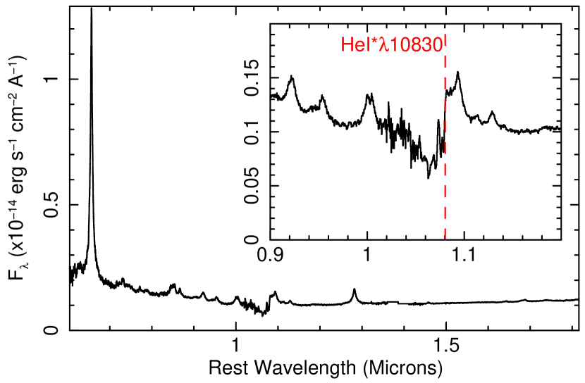
Figure 1: IRTF SpeX spectrum of FBQS J1151$+$3822. The inset shows the area of the He I*$\lambda 10830$ absorption line, where the vertical line shows the rest wavelength of He I*$\lambda 10830$.

The infrared spectroscopic observations were made at the NASA Infrared Telescope Facility (IRTF) using the SpeX spectrograph (Rayner et al., 2003) in the short cross-dispersed mode (SXD) with an effective bandpass of 0.8–2.4$\rm\,\mu m$ as part of another project. The observations were made 2008 March 28–30 and 2008 August 22–24. Conditions were non-photometric. As noted above, the scope of this paper is limited to the He I absorption, and so we will defer the detailed description of the observations and reduction to Barber et al. (in prep.) which will include analysis of the entire dataset. For this paper, we use the spectra from FBQS J1151$+$3822, PG 1543$+$489, PHL 1811, and FBQS J1702$+$3247; these were all observed with a 0.8” slit for effective exposures of 2, 1.7, 2.9 and 1 hour(s) respectively. Flat-field lamps and line lamps were observed along with each object. A nearby early A-type star was also observed along with each object. The spectra were reduced using the IDL software SpexTool (Cushing et al., 2004). The flux calibration and correction for telluric features was performed using the A star spectrum and employing distributed IDL software that use the methods described in Vacca et al. (2003). In the vicinity of the He I absorption feature (at approximate 1.4$\rm\,\mu m$ in the observed frame), the FWHM resolution measured from the line-lamp spectra ranged from $\sim 350$ to $\sim 400\rm\,km\,s^{-1}$ at the short wavelength end of the 4th spectral order to $\sim 300\rm\,km\,s^{-1}$ at the long wavelength end of the 5th spectral order. The spectrum is shown in Fig. 1.

The short wavelength end of the absorption feature occurs at the long wavelength end of the 5th spectral order. There is a prominent telluric absorption band between $\sim 1.35$ and $1.45\rm\,\mu m$. In addition, the effective area is dropping off at the end of the order. Unfortunately, our feature is partially compromised by these issues. Is it possible that the absorption feature is somehow an artifact of the data reduction? This is not likely, primarily because the long wavelength end of the absorption feature is found on both the long wavelength end of the 5th spectral order, and on the short wavelength end of the 4th spectral order, and both have the precisely the same shape. In addition, FBQS J1151$+$3822 is a relatively bright quasar for the IRTF, and the telluric correction method is very reliable (Vacca et al., 2003).

The spectra were corrected for Galactic reddening using $E(B-V)=0.023$ (derived from the infrared cirrus, Schlegel et al., 1998) using the CCM reddening curve (Cardelli et al., 1989). The redshifts were derived from the IRTF spectra assuming that H$\alpha$, Paschen $\beta$ and Paschen $\alpha$ are observed at the rest wavelengths. For FBQS J1151$+$3822, PG 1543$+$489, PHL 1811, and FBQS J1702$+$3247, the redshifts were found to be 0.3354, 0.4104, 0.1928, and 0.1644, respectively. These are insignificantly different from the values listed in NED. The spectra were shifted into the rest frame using these redshift values. Finally, the spectra were modestly smoothed.

2.2 Derivation of the He I$\lambda 10830$ Apparent Optical Depth

As discussed in e.g., Savage & Sembach (1991), the apparent optical depth of an absorption feature is given by $\tau(\lambda)=\ln[I_{0}(\lambda)/I_{obs}(\lambda)]$, where $I_{obs}(\lambda)$ is the observed spectral intensity, and $I_{0}(\lambda)$ is the unabsorbed spectral intensity. The IRTF spectrum of FBQS J1151$+$3822 yields $I_{obs}(\lambda)$, of course. In order to obtain the apparent optical depth, we need to obtain the intrinsic continuum $I_{0}$. The lines in the near IR spectra of quasars are relatively unblended, compared with the optical and near UV bands; however, the continuum in this region of the spectrum transitions from the AGN power law at longer wavelengths to the dust-reprocessing feature at shorter wavelengths (Fig. 1). In FBQS J1151$+$3822, it appears that this change in the continuum occurs very near the absorption feature.

To obtain $I_{0}$, we used the following procedure. First, we determined that of the 12 objects that we observed, PG 1543$+$489, PHL 1811, and FBQS J1702$+$3247 had spectra most similar to that of FBQS J1151$+$3822 outside of the absorption region. In addition, we downloaded the spectra presented by Landt et al. (2008) and found two additional objects that resemble FBQS J1151$+$3822: PDS 456 and HE 1228$+$013. The spectra were similar to that of FBQS J1151$+$3822 in terms of emission lines, but different in their continuum slopes. We used line-free regions in FBQS J1151$+$3822 and each of the comparison objects to determine power laws that the comparison-object spectra could be divided by so that their continua would match that of FBQS J1151$+$3822. We then performed this continuum transformation.

The procedure above works quite well for the continuum correction. However, several of the objects have significantly higher equivalent widths than FBQS J1151$+$3822. To scale the lines, we need to divide each spectrum by its continuum. We focus on a limited wavelength range between 0.79 and 1.4$\rm\,\mu m$ and fit the line-free continuum bands of each object with a 4th order polynomial. Each spectrum was then divided by this polynomial. Finally, the spectra were suitably scaled. The following scale factors were used: PG 1543$+$489: 0.73; PHL 1811: 1.1; FBQS J1702$+$3247: 0.75; PDS 456: 1.0; HE 1228$+$013: 0.61. The results are shown in Fig. 2.

The figure shows that all objects are rather similar over most of the range shown except for the long-wavelength side of the He I/Pa$\gamma$ feature. In particular, in the region of the absorption feature which is seen to stretch between 1.044 and 1.082$\rm\,\mu m$, most objects are quite similar except for PDS 456 which is seen to exhibit some strange feature near 1.07 microns (Landt et al., 2008). Since PHL 1811 has by far the best signal-to-noise ratio of all of the spectra presented, we use the scaled version shown in Fig. 2 as the intrinsic spectral intensity $I_{0}$. Except for PDS 456, the other spectra match that of PHL 1811 within about 5%, and we take that value as the systematic uncertainty in our estimate of $I_{0}$.

The resolution of the IRTF spectra in the region of the feature is about $350\rm\,km\,s^{-1}$. Binning the FBQS J1151$+$3822 spectrum by a factor of two yields slightly more than two bins per resolution element. The PHL 1811 spectrum was resampled on the same wavelengths as the FBQS J1151$+$3822 spectrum.

The IRTF spectra were were extracted using the optimal extraction technique (Cushing et al., 2004). This method produces statistical errors that appear to be too small. Specifically, the standard deviation in the data in relatively flat and smooth regions of the continua are systematically several factors larger than the assigned errors. To account for this trend, we increase the size of the error bars by a factor of 6 for the PHL 1811 spectrum, and a factor of 4 for the FBQS J1151$+$3822 spectrum. Then, between 1.0 and 1.1 microns, in the region of the absorption feature, the signal to noise ratios range between about 16 and 130 for the FBQS J1151$+$3822 spectrum and are about 200 uniformly for the PHL 1811 spectrum.

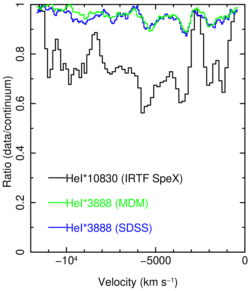
Figure 3: The ratio of the data to the continuum ($R$) is shown for the He I*$\lambda 10830$ and the He I*$\lambda 3889$ lines. The apparent optical depth is $\tau=-\ln R$. The ratios are similar for the two lines, but not identical, implying the presence of velocity-dependent optical depth and covering fraction. On the linear part of the curve of growth, the optical depth of He I*$\lambda 3889$ should be 23.3 times lower than that of He I*$\lambda 10830$. It is clearly higher than that, implying the presence of partial covering.

Using these spectra, the ratio and apparent optical depth were computed as a function of velocity. The resulting ratio is shown in Fig. 3. The maximum velocity $v_{max}$ is $\sim 11,000\rm\,km\,s^{-1}$, showing that FBQS J1151$+$3822 is truely a broad absorption line quasar.

2.3 Optical Observations

We analyzed two optical spectra of FBQS J1151$+$3822. The Sloan Digital Sky Survey observed the object 2005 March 11 for 4600.4 seconds. The spectrum was extracted from the archive, rewritten in text format, and a moderate amount of smoothing was applied as mentioned in §2.1. The SDSS redshift was $0.3351\pm 0.002$. We remeasured the redshift using the Balmer lines and estimated it to be 0.3341. The spectrum was corrected for redshift and reddening as above.

The object was also observed at the MDM observatory 2.4 meter Hilter telescope and the CCDS spectrograph on January 3, 2009 for 1 hour. We used a grating with $350\,\rm mm^{-1}$ and a 1” slit yielding observed-frame spectra between $\sim 4300$Å and $\sim 5800$Å. Conditions were non-photometric. The spectra were reduced in a standard way independently using MIDAS (MD) and IRAF (KML, SB); the results were consistent. The signal-to-noise ratio of the FBQS J1151$+$3822 was estimated to be approximately 70. The FWHM resolution in the vicinity of the He I$\lambda 3889$ line was found to be about $175\rm\,km\,s^{-1}$ from the line lamps.

2.4 Derivation of the He I*$\lambda 3889$ Apparent Optical Depth

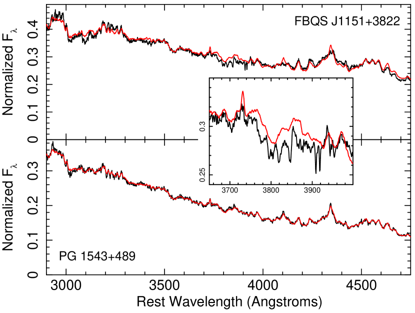
Figure 4: Fitting the optical spectra to the template model. Top: the SDSS FBQS J1151$+$3822 spectrum fitted with the template created from 28 SDSS spectra excluding the region of the absorption lines. The MDM spectrum yields a similar result but with a smaller wavelength range (3200–4400Å). Bottom: The SDSS spectrum from PG 1543$+$489 fit with the same model for comparison. Inset: the region of the FBQS J1151$+$3822 spectrum in the vicinity of the absorption lines.

Extraction of the apparent optical depth of the He I*$\lambda 3889$ feature from either the SDSS or MDM spectrum is challenging. First, as can be seen in Fig. 4, the apparent optical depth of the 3889 Å feature is quite small. This is expected, since the ratio of $f_{ik}\lambda$ between the 10830 and 3889Å components is 23.3, which means that on the linear part of the curve of growth, the true optical depths of these lines should have the a ratio of 23.3 (Savage & Sembach, 1991). Second, the continuum is not a power law; rather, FBQS J1151$+$3822 is a strong Fe II emitter and the continuum includes a forest of Fe II lines. In fact, to the casual observer, the only clearly apparent absorption lines are the Ca II H&K lines. Without knowing that there is a 10830Å absorption trough in this object, the He I lines are easily confused with the Fe II continuum. Thus, FBQS J1151$+$3822 had never before been recognized to be a BALQSO.

We need a suitable estimation of the Fe II continuum to extract the optical depths. The usual I Zw 1 template (Boroson & Green, 1992) is inadequate because it does not cover the shorter wavelengths around He I*$\lambda 3889$ that we need, so we developed a template from SDSS spectra. We selected a sample of 28 bright low-redshift quasars that have sufficiently narrow lines that the Fe II complexes near H$\beta$ are resolved. From these, we constructed an average line spectrum as follows. The spectra, de-reddened and transformed to the rest frame, were resampled onto a common wavelength range between 2869Å (the lower wavelength limit of the SDSS spectrum of FBQS J1151$+$3822) and 4750Å (considered the upper limit to avoid H$\beta$, as that line can be quite variable between objects). The spectra were normalized by dividing by the average flux obtained from a 21-element bin located in the middle of the chosen wavelength range. The power law slope of the continuum was estimated by fitting a power law to the flux in line-free bands, and all spectra were normalized using this estimated value to slope of 1.96 (i.e, where $F(\lambda)\propto\lambda^{-1.96}$). At each wavelength, the mean spectrum was computed, and finally, the power law estimated from the line-free bands was subtracted yielding an average line spectrum.

The SDSS and MDM spectra were then fitted using this Fe II line model excluding the regions where absorption lines, both originating in He I and Ca II, may be present. For the SDSS spectrum the excluded regions were 3015–3188.7Å and 3678–3958 Å. For the MDM spectrum, with its more limited wavelength coverage, only the second region was excluded. Four parameters were fit: the reddening of the input spectrum (i.e., the observed spectrum was dereddened by an input amount), the power law index, the power law normalization, and the line normalization. A figure of merit was computed at each grid point, and the minimum of the grid identified the best fit. The figure of merit used was the absolute value of the difference between the unreddened input spectrum, and the power law plus line flux model, divided by the unreddened uncertainty in the case of the SDSS spectrum (the MDM spectrum, produced by IRAF, had no formal uncertainties).

The SDSS spectrum includes a notable feature between $\sim 3200$–3300Å probably originating in Fe II multiplets M6 and M7 (Phillips, 1978, e.g.,). The shape of the iron continuum varies from object to object in the UV (e.g., Leighly et al., 2007) and so it is possible that it also varies in the optical. We therefore create an alternative line spectrum from seven of the 28 objects which shows the largest excess variance between 3170–3300 Å. A large value of excess variance chooses objects which both have prominent features and good signal-to-noise ratios. We then fit the MDM and SDSS spectra with this alternative Fe II continuum.

It is clear that the uncertainty in the results produced by the procedure described above will be dominated by the systematic errors associated with the fact that the Fe II spectrum is not identical among AGNs. An estimate of the systematic error can be obtained from the standard deviation of the mean spectrum from the sample used to create the Fe II continuum. The standard deviation in the region of the absorption feature has an offset due to normalization offsets in the average spectra, plus fluctuations with scales of tens of angstroms with an amplitude of about 2%. The offset is unimportant since the fitting routine will remove uncertainty associated with that. However, the fluctuations in the standard deviation are important since they measure the differences in the spectrum among AGN. Thus, we assign a systematic uncertainty of 1% to the model spectrum. The statistical uncertainty in the SDSS spectrum in the region of interest is about 2%. Thus the ratio will have an uncertainty of about 2.2%, and the apparent optical depth should have an uncertainty of about the same value. Based on the number of counts in the MDM raw spectrum, we estimate a statistical uncertainty of about 1.5%. Propagating our estimated 1% uncertainty in the model spectrum yields an uncertainty in the ratio for the MDM spectrum of about 1.8%. The results of fitting the 28-SDSS-spectra model to the SDSS spectrum of FBQS J1151$+$3889 are shown in Fig. 4; the other combinations of spectra and Fe II model were similar. The resulting ratio of data to model for the SDSS and MDM spectra are shown in Fig. 3.

In principle, we should also observe He I*$\lambda 3188$ absorption in the SDSS spectrum. But $\lambda f_{ik}$ is 79.4 times smaller for that component than that of He I*$\lambda 10830$, so it is expected to be even weaker than He I*$\lambda 3889$, where the $\lambda f_{ik}$ ratio is 23.3. Furthermore, the region of the spectrum around 3188Å has exceptionally strong and complex Fe II emission in it. In addition, the Fe II emission in this region seems to vary from object to object more profoundly than it does around 3889Å. So while there is some suggestion of absorption in this object (Fig. 4), we cannot robustly extract an apparent optical depth profile and therefore ignore this line for the rest of the analysis.

2.5 Balmer Absorption Optical Depth Upper Limit

We do not see any significant Balmer line absorption in these spectra. However, it may be present at low equivalent widths. We fitted the SDSS spectrum in the vicinity of the H$\alpha$ emission line with a power law continuum, a Lorentzian profile for the Balmer line, two Fe II templates (which will be described in Leighly et al. in prep.), and the optical depth profile obtained from the He I* $\lambda 10830$ absorption line. The resulting component was transformed to a ratio as a function of velocity, which could be used to estimate the Balmer column density upper limit (§2.8).

The MDM spectral bandpass did not cover H$\alpha$. The IRTF bandpass does (Fig. 1), but the spectrum had lower signal-to-noise ratio in the vicinity of this line compared with the SDSS spectrum. Therefore, we use the limit obtained from the SDSS spectrum henceforth.

2.6 Ca II H& K Absorption

Ca II H&K absorption lines are visible in the optical spectra. There are two relatively narrow ($\sim 300\rm\,km\,s^{-1}$ FWHM) features that peak at $\sim-1200\rm\,km\,s^{-1}$ and $\sim-2000\rm\,km\,s^{-1}$. Both sets of features lie redward of the He I* absorption.

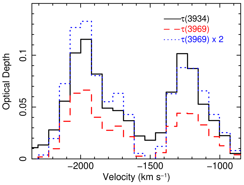
Figure 5: The apparent optical depth of the Ca II H&K absorption feature. The optical depth from the 3934Å component and the 3969Å component are shown. The ratio of $\lambda f_{ik}$ for the two components is approximately 2. We find that $2\times$ the apparent optical depth of the 3969Å component approximately matches that of the 3934Å component. This implies that partial covering is not important and that the true optical depth is equal to the apparent optical depth.

These two features have low apparent optical depth and are a challenge to analyze. We begin with the ratio of continuum to model derived in §2.4 for the MDM and SDSS spectra obtained using the two models for the Fe II emission discussed in §2.4. The MDM and SDSS profiles appear consistent, so we average the ratios for each Fe II model, leaving us with two spectra. We extract the apparent optical depths from both and display the results for the 28-spectrum Fe II model in Fig. 5.

Ca II is a lithium-like ion and like other resonance transitions in lithium-like atoms, the $\lambda f_{ik}$ for the 3934Å component is about 2 times that of $\lambda f_{ik}$ for the 3969Å (actually equal to 2.05). We found that the apparent optical depths shown in Fig. 5 appear to have a ratio of 2:1, and indeed, if we double the apparent optical depth of the 3969Å component (dashed line in Fig. 5) we find a good correspondence with the apparent optical depth of the 3934Å component (solid line). This implies that partial covering is not important for these lines and that they are not saturated. Indeed, if we use the apparent optical depth profiles to estimate the column density of Ca⁺ ions, we find that the measured column density from the two lines among the two spectra ranges between $9.4\times 10^{12}\rm\,cm^{-2}$ and $1.07\times 10^{13}\rm\,cm^{-2}$. These estimates are consistent, given the uncertainties on the ratio spectra. We take the mean of these estimates ($1.0\times 10^{13}\rm\,cm^{-2}$) to be the column density of the Ca⁺ ions.

We believe that this absorption arises in different gas than the He I* absorption. First, the He I* absorption profile is much broader; had that broad profile been present in the Ca II lines, the 3969Å component would have severely altered the 3934Å component, as these two lines are separated by only $2655\rm\,km\,s^{-1}$. Likewise, the 3934Å component would have altered the low velocity region of the He I* line, and strong absorption would have been seen between the He I*$\lambda 3889$ and the Ca II$\lambda 3934\AA\/$ lines (separated by $6100\rm\,km\,s^{-1}$). These features are not seen. In addition, the Cloudy simulations discussed in §3.1 for the relatively high-ionization He I* lines do not produce significant Ca⁺ column density. The highest log column density predicted is $\log N_{Ca+}=12.3$, a factor of five too low; the highest column densities are found at the lowest ionization parameters. Generally speaking, the ionization parameter is higher and the column density is lower in our simulations than is generally required for Ca II absorption (e.g., Hall et al., 2003). Our interest in this paper is in the He I* lines, and we do not discuss the Ca II absorption further.

2.7 Column Density Lower Limits

As discussed by Savage & Sembach (1991) and others, the optical depth is related to the ratio of the observed continuum $I(\lambda)$ to the true continuum $I_{0}(\lambda)$ by

$$\tau(\lambda)=\ln[I(\lambda)/I_{0}(\lambda)].$$

If the absorption line is not saturated and the absorber fully covers the source, the column density of the absorbing ion can be obtained from the optical depth (e.g., Savage & Sembach, 1991)

$$N=\frac{m_{e}c}{\pi e^{2}f\lambda}\int\tau(v)dv$$

where $m_{e}$ is the mass of the electron, $c$ is the speed of light, $e$ is the charge on the electron, $f$ and $\lambda$ are the oscillator strength and wavelength for the transition, respectively, and $v$ is the velocity relative to the rest frame with respect to $\lambda$.

Using the ratio profiles discussed in §2.2, and 2.4, we find that the log of the column density of HeI* is $\sim 14.3$ from the He I*$\lambda 10830$ line, and $\sim 14.75$–$14.95$ from the various spectra for the He I*$\lambda 3889$ line. These two estimates do not agree, although physically they have to be equal. This means that the assumption that the absorber fully covers the source is incorrect, and a partial covering analysis is appropriate (§2.8).

We discuss the Balmer absorption limit in the next section.

2.8 Partial Covering Analysis

HeI*$\lambda 10830$ and HeI*$\lambda 3889$ are transitions from the same lower level. Therefore, the ratio of optical depths is fixed by atomic physics, provided that the lines are not saturated. We can use these ratios to solve for the parameters of a two-parameter inhomogeneous absorption model as a function of velocity. The simplest example is the partial covering model, where

$$R_{10830}=(1-C_{f})+C_{f}e^{-\tau_{10830}}$$

$$R_{3889}=(1-C_{f})+C_{f}e^{-\tau_{3889}}$$

where $R$ is the ratio of the observed spectrum to continuum, $C_{f}$ is the covering fraction, and $\tau_{10830}$ and $\tau_{3889}$ are the true optical depths. All of these parameters are functions of velocity (e.g. Sabra & Hamann, 2005). We can solve these equations for $C_{f}$, $\tau_{10830}$ and $\tau_{3889}$, subject also to the constraint that $\tau_{10830}=23.3\tau_{3889}$.

Partial covering models have been widely applied to quasar spectra. One of the first applications was reported by Hamann et al. (1997), who analyzed metal resonance lines which have $\tau$ ratios very close to 2. In that case, the two equations can be reduced to one analytically. For our $\tau$ ratio, an analytic expression cannot be derived. We found that the following method worked most reliably. First, we computed a grid of simulated $R_{10830}$ and $R_{3889}$ for a large range of input covering fractions and $\tau_{3889}$ (specifically, 5001 covering fraction points between 0 and 1, and 4001 logarithmically-spaced $\tau_{3889}$ points between 0.01 and 100). Then for each velocity, we determine which pair of $(C_{f},\tau_{3889})$ best matches the data, where our figure of merit is $\chi^{2}$; specifically, $\sqrt{(D_{3889}^{2}+D_{10830}^{2})}$ and the $D$ values are the difference between the data points and the models divided by the uncertainty in the data points. At the point where the figure of merit is minimized, we evaluate an uncertainty on the model point where the confidence criterion is our best fitting $\chi^{2}$ plus 1.0, corresponding to $1\sigma$ for one parameter of interest, in the direction along the parameter axis. Note that the best-fitting $\chi^{2}$ values were all very small fractions of 1 since we have two equations and two unknowns, essentially, and since our grid was finely meshed. Finally, we exclude points that are unphysical, where $R_{3889}>R_{10830}>R_{3889}^{23.3}$ is not obeyed (e.g., Hamann et al., 1997). Generally, this amounts to only a few points; i.e., of the 69 points in the velocity profile, 5–8 points are rejected (Table 1).

Fig. 6 shows the results for the IRTF ratio for the He I*$\lambda 10830$ line and the SDSS spectrum fit with the 28–SDSS-spectrum Fe II model for the He I$\lambda 3889$ line; the others were similar. The top panel shows the data and the model fit. The second panel shows the optical depth for the 3889Å line; the value for the 10830Å line would be 23.3 times larger. The third panel shows the covering fraction as a function of velocity. The fourth panel shows the incremental column density as a function of velocity (e.g., Savage & Sembach, 1991) computed from the average $\tau$, i.e., the value integrated over the spatial dimension (e.g. Arav et al., 2005). For the partial covering model, $\bar{\tau}=C_{f}\tau$. The uncertainties in the incremental column density are conservatively estimated from the products of the limits of the optical depth and covering fraction.

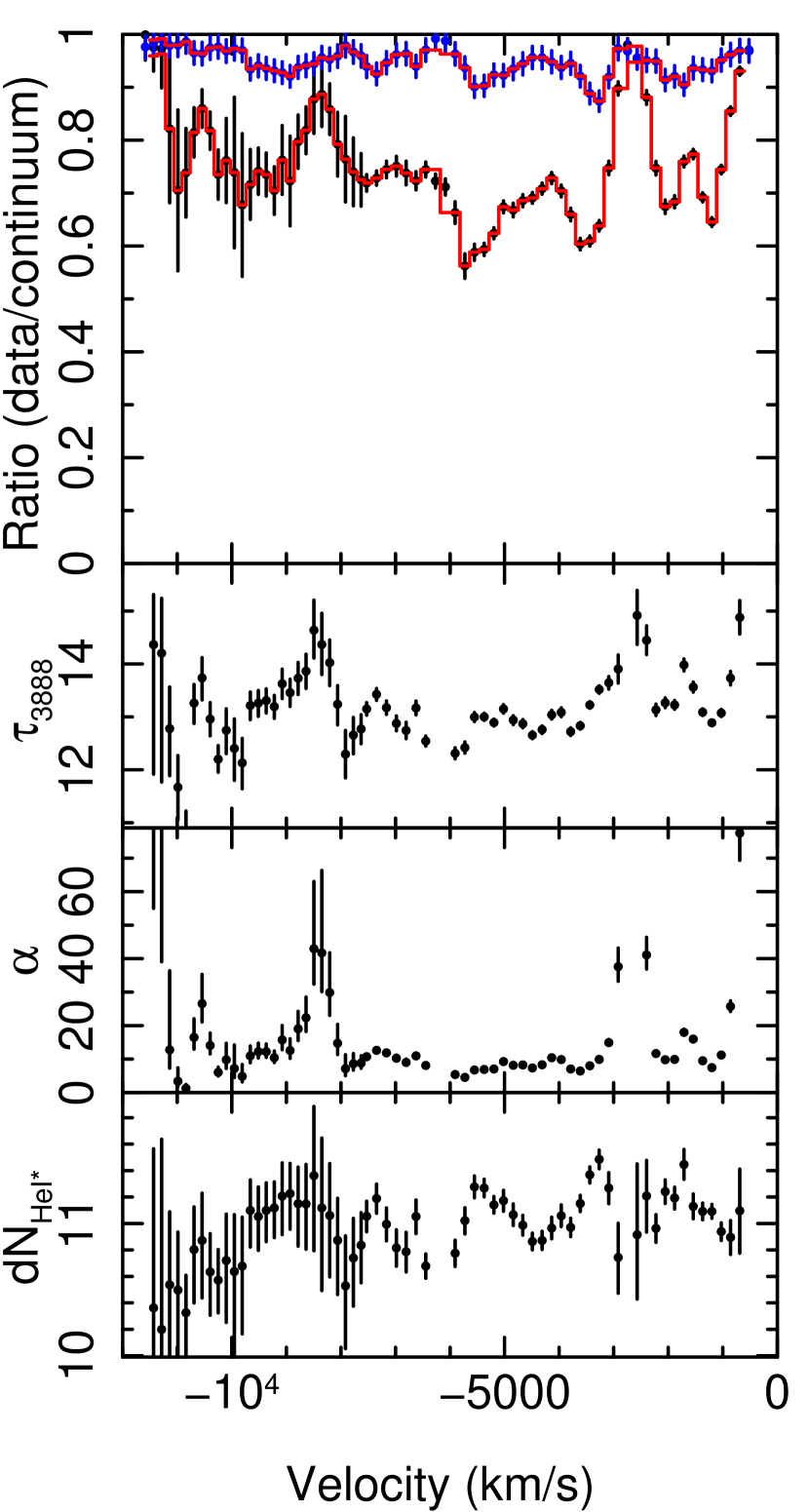
Figure 7: Power law inhomogeneous absorber model of the IRTF ratio and the SDSS ratio extracted using the 28-spectrum Fe II model. The results for the excess-variance Fe II model and for the MDM ratio spectrum are similar. The top panel shows the ratios with the model overlaid. The second and third panels show the fitted optical depth and power law index. The bottom panel shows the incremental column density as a function of velocity computed from the average optical depth.

The simple partial covering model, above, posits a physical scenario where $1-C_{f}$ of continuum source is seen directly, while $C_{f}$ of the source is uniformly covered by gas with a single value of $\tau$. This scenario may be appropriate in some cases, for example, when a fraction of the continuum is scattered into our line of sight by electrons located in the vicinity of the symmetry axis; the presence of these electrons is indicated by the large polarization frequently seen in the absorption troughs (e.g., Ogle, 1998). But it is also possible that the optical depth is not uniform over the source. These so-called inhomogeneous absorbers have been discussed by e.g., De Kool et al. (2002), Sabra & Hamann (2005), and Arav et al. (2005). We choose investigate the power law inhomogeneous absorber model. We use a power law function, i.e., $\tau(x)=\tau_{max}x^{a}$, where $\tau_{max}$ and $a$ are fit parameters. We use the analytical formula for the ratio of the data to model given in Sabra & Hamann (2005) (their equation 14), and follow the approach outlined above. Our model grid consisted of 3501 values of $a$ spaced logarithmically between 0.0316 and 100, and 4001 values of $\tau_{max}$ spaced logarithmically between 0.01 and 100. The resulting fit for the IRTF spectrum and the SDSS spectrum fit with the 28-spectrum Fe II model is shown in Fig. 7. In this case, the average optical depth is $\tau_{max}/(a+1)$. The upper limit on the column density was conservatively estimated using the upper limit on $\tau_{max}$ divided by the lower limit on $a$; similarly, the lower limit was estimated using the lower limit of $\tau_{max}$ and the upper limit of $a$.

For both models, the total He I* column density is obtained by integrating over the the average $\tau(v)$ profile (e.g., Savage & Sembach, 1991), and the uncertainties obtained by integrating over the upper and lower bounds. The results are given in Table 1. The values for the partial covering model and power law model are essentially identical. In addition, the values are very similar among the four different He I*$\lambda 3889$ ratio profiles. The average of the log of the eight column density estimates is 14.9. This is the value that we use for Cloudy simulations and the remainder of the paper.

The derived value of He I* column density is very similar to the lower limit derived from the 3889Å component (§2.7; Table 1). This is not an accident. To obtain the lower limit, we assume

$$R_{s}\approx exp(-\tau_{s})$$

for the weaker component, for example. As noted above, the partial covering model is

$$R_{s}=(1-C_{f})+C_{f}\exp(-\tau_{s}).$$

If the optical depth of the weaker component is sufficiently small, the exponent can be Taylor expanded, as follows:

$$R_{s}\approx(1-C_{f})+C_{f}(1-\tau_{s})=1-C_{f}\tau_{s}.$$

Inverting the Taylor expansion, we find that

$$R_{s}\approx exp(-C_{f}\tau_{s})=exp(-\bar{\tau_{s}}).$$

Thus, for sufficiently low optical depth, the apparent optical depth is approximately equal to the average optical depth.

We use this fact to derive the upper limit on the column density of the hydrogen $n=2$. As discussed in §2.5, there is no apparent Balmer line absorption in this object, and we treat the observed small optical depth as a lower limit. Needless to say, the optical depth is very small. Thus, we can assume that the apparent optical depth is approximately equal to the average optical depth. Next, we need the oscillator strength for the Balmer absorption line. The sum of the oscillator strengths for the 2s state is 0.44 and the sum for the 2p state is 1.42. If the $n=2$ Hydrogen is distributed among the 2s and 2p states according to their oscillator strengths, we obtain an estimate of the log of the hydrogen $n=2$ column equal to 12.9. But there is no permitted transition to ground from the 2s state, so one might expect that it be more highly populated than the 2p state. If all the absorption lines were from 2s only, we would obtain an estimate of the log of the Hydrogen $n=2$ column equal to 13.5. In the Cloudy modeling, we can separate hydrogen $n=2$ in the 2s state and in the 2p state, and we will adjust the hydrogen $n=2$ column upper limit according to the fraction predicted in these two states. We discuss this in the next section.

3 Cloudy Modeling

3.1 Ionization Parameter, Density and Hydrogen Column Density Constraints

Armed with our estimates of the He I* column density and hydrogen $n=2$ column density upper limit, we can proceed to use these to constrain the properties of the absorbing gas. We use Cloudy 08.00, last described by Ferland et al. (1998). Initially, we used the so-called Cloudy AGN continuum with the same parameters as used by Korista et al. (1997); this is taken to be a typical AGN continuum. We examine a wide range of ionization parameters ($-2.0\leq\log U\leq 1.2$) and densities ($3.0\leq\log n\leq 9.0$). We use the full Fe II model (i.e., 371 levels; Verner et al., 1999) for every run. He I* is populated essentially solely by recombination of He⁺, and therefore, we expect the metastable state of the He I ion to be coincident with He⁺. Therefore, initially, we set the column density equal to $\log N=24.5+\log U$; this integrates through the hydrogen ionization front and therefore certainly through the entire He⁺ region.

The column density of He I* can be obtained from the output in two ways. First, the total column density can be output using the punch some column densities command Second, the fraction of helium in different states in every calculational zone can be output if the print every command is used. The fraction can be converted to a density using the helium abundance; it can then be integrated over depth. We process our Cloudy results by first obtaining the log of the total He I* column density and determining whether or not it is greater than or equal to 14.9. If it is not, that combination of ionization parameter and density are rejected. If it is, we interpolate to determine the thickness of the gas required to reach a log He I* column density of 14.9. Using the gas density and this thickness, we obtain the total hydrogen column density. We then run a second set of Cloudy models as a function of ionization parameter and density in which the total column density is set to the value estimate from the depth and density.

The density as a function of depth of hydrogen in various levels such as $n=2$ s and p can be output using the punch hydrogen populations command. The output of the second set of runs is examined and the total column density of hydrogen in the the 2s and 2p states is computed. The upper limit constraint is computed based on the fraction of the $n=2$ hydrogen in the two states. If the amount exceeds the limit, that combination of ionization parameter and density is rejected. It is interesting to note that we can’t combine this step with the previous one because the density of hydrogen in $n=2$ differs whether it is in the middle or back side of the cloud, as a consequence of radiative transfer.

The results are shown in Fig. 8. Solutions at low ionization parameter are rejected because they fail to produced sufficient He I*. Basically, for solutions with the lowest allowed ionization parameter, we are integrating through the entire He I* zone. For higher ionization parameter solutions, we integrate only part of the way through the He I* zone. Solutions at high density are rejected because they produce too much $n=2$ hydrogen. The inferred log hydrogen column density is larger than 21.6 and may be as large as 23.8, or even larger, although it should be noted that Thompson scattering becomes important for the higher column densities. The ionization parameter is greater or equal to $\log U=-1.4$.

The total hydrogen column density inferred, as well as the extent of the allowed $\log U$–$\log n$ parameter space, will also depend on the shape of the input spectral energy distribution, the metallicity of the gas, and whether or not the gas has a differential velocity field (i.e., turbulence). The effect of these factors is discussed in the Appendix.

How do these results compare with results from studies of BALQSOs? Dunn et al. (2010) compile a collection of results from analyses of 8 quasars where partial covering has been taken into account. The range of column densities in their Table 9 is 19.9–22.2; however, our minimum value is larger than all but two. Dunn et al. (2010) find a range of $\log U$ between $-3.1$ and $-0.7$; our object has a larger ionization parameter than all but three. But these objects were not chosen as high-column candidates. Hamann (1998) report analysis of the P V quasar PG 1254$+$047. They find, for solar metallicity, that $\log U>-0.6$ and $\log N_{H}>22$. These values are larger than our minimums, but we note that if the ionization parameter were $\log U=-0.6$, then the column density would be $\sim 22.3$, larger than Hamann (1998)’s estimated lower limit. Thus, it appears that FBQS J1151$+$3822 is a high-column BALQSO. In addition, as we will discuss later, these results suggest that He I* is useful to constrain high-column outflows.

3.2 Additional Constraints Possible with UV Spectra

Our solutions encompass a fairly large range of ionization parameter-density parameter space. Is it possible to constrain the solution better? Certainly, we cannot with our current spectra, limited, as they are, to the rest optical and infrared bandpass. However, the rest UV offers numerous transitions that may produce absorption in FBQS J1151$+$3822.

Which ions could help us constrain $\log U$–$\log n$ parameter space? Ideally, we need ions that have column densities large enough to make detectable absorption lines, but not so large that the lines become saturated. Savage & Sembach (1991) show that the optical depth as a function of velocity is $\tau(v)=2.654\times 10^{-15}f_{ik}\lambda N(v)$. This equation has to be integrated over velocity; in our case, the column-weighted mean velocity is $\sim 5500\rm\,km\,s^{-1}$, so we multiply $\tau(v)$ by that value to estimate the integrated column density. Many of the resonance lines of interest have total $f_{ik}\sim 0.3$–1.0, and the lines are in the UV, so $\lambda$ is of the order of, say, 1500Å. Then, a ratio of observed to continuum of $\sim 0.5$ corresponds to a column density of $\sim 2\times 10^{15}\rm\,cm^{-2}$. The natural log of the ratio is correlated with the column density. So a 10-times higher column density would yield a ratio of $\sim 0.001$, and the line would be saturated. Thus, for the commonly observed resonance lines (e.g., C IV), an ionic column around $10^{16}\rm\,cm^{-2}$ would be likely to be saturated. Likewise, a column density 10 times lower would produce a ratio of 0.93, and as we saw with He I*$\lambda 3889$, such a weak absorption line would be somewhat difficult to detect. So we are looking for ions with log column densities in the vicinity of $14.7$ to $16$. This analysis of course breaks down for transitions with lower oscillator strengths; such lines could be detected at higher column densities.

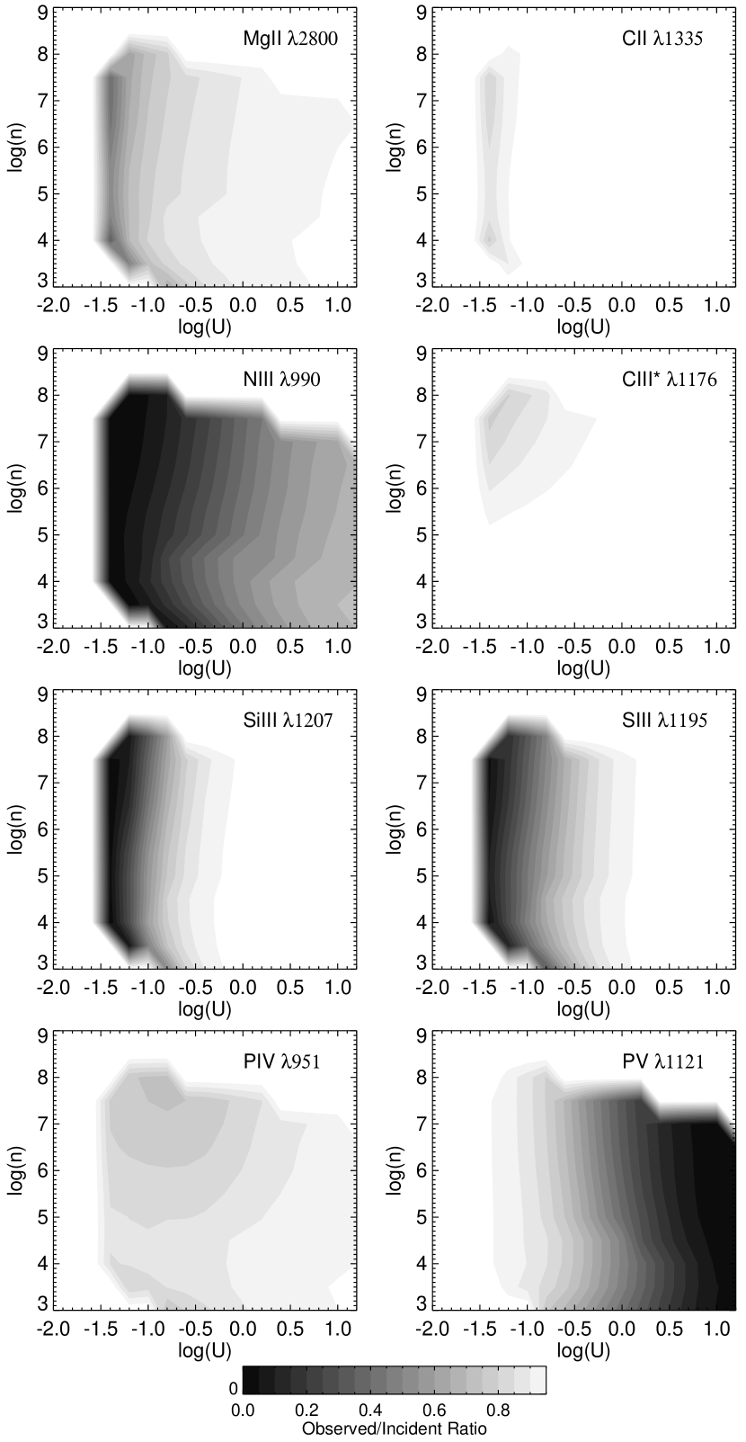
Figure 9: Contours of the ratio of the predicted intensity divided by the continuum intensity for column densities obtained from the Cloudy modeling. The optical depth has been spread over a range of 11,000$\rm\,km\,s^{-1}$ appropriate for the line profile in this object. Transitions that are shown are neither saturated nor too weak to be observed; they can in principle remove the degeneracy in the modeling by constraining ionization parameter and density.

We use Cloudy models to estimate the ratio of spectrum to continuum by making use of the fact that $I/I_{0}\approx exp(-\bar{\tau})$ and $\tau(v)=2.654\times 10^{-15}f_{ik}\lambda N(v)$ (Savage & Sembach, 1991) where $N(v)$ is the ionic column density as a function of velocity in the units of $\rm cm^{-2}$ per $\rm kms^{-1}$. The total ionic column densities are obtained from the Cloudy models. To estimate $N(v)$, we make the approximation that the total column density is equally distributed in velocity space over the $11,000\,\rm km\,s^{-1}$ absorption line. We examined most of the lines predicted to be bright in quasar absorption systems by Verner et al. (1994) for wavelengths longer than 900Å. He I* is essentially a high-ionization line, and many low-ionization species have low column densities and are predicted to produce essentially no absorption lines. A few, including C II, Al III, and Si II, are predicted to produce weak lines for the lower ionization parameter range, but none at the higher ionization parameters. Others, such as the resonance lines of C III, C IV, N V, O VI, and Si IV, are expected to be saturated. But some lines fall mid-way between these two extremes, showing strong evolution in ratio as a function of ionization parameter, and in some cases, also dependence on density. The most important of these (plus C II as an example of a line expected to be present only at lowest ionization parameters) are shown in Fig. 9.

3.2.1 Ionization Parameter and Density Discrimination

Fig. 9 has several intriguing features. First, several of the lines, including Mg II$\lambda 2800$, C II$\lambda 1335$, N III, Si III$\lambda 1206$, and S III$\lambda 1195$ decrease with increasing ionization parameter, while P V$\lambda 1121$ increases with increasing ionization parameter. This suggests that observing P V with along with e.g., N III$\lambda 990$, would allow us to constrain the ionization parameter. The ionization parameter is degenerate with the total column density (Fig. 8), so this would be an important constraint for this outflow.

Several lines in this bandpass are expected to have density dependence, and the Cloudy simulations verify that expectation. S IV$\lambda 1063$ was observed in WPVS 007 and the properties of this line were discussed in Leighly et al. (2009). As noted in that paper, S IV is composed of three components. The ground state transition has a wavelength of 1062.7Å. The other two transitions from this configuration arise from an excited state with $E_{i}=951.43\,\rm cm^{-1}$, with wavelengths of 1072.96 and 1073.51Å. Population of the upper level requires $n_{e}>A_{ki}/q_{ki}$ where $A_{ki}=7.70\times 10^{-3}$ is the Einstein A value for the transition from the excited state to the ground state, resulting in the S IV $10.51\rm\,\mu$ line, and $q_{21}$ is the collision deexcitation rate, which can be found from the collision strength $\Upsilon$ for this transition. For a nebular temperature of 15,000 K, Saraph & Storey (1999) give $\Upsilon($S IV)$=8.48$. The resulting critical density is $n_{crit}=4.7\times 10^{4}\,\rm cm^{3}$. At densities above critical, the ratio would approach $g_{ik}(excited)/g_{ik}(ground)=2.02$. This suggests that observing S IV would allow us to pin down the density of the gas. Unfortunately, this line is predicted to be saturated in this object.

The C III*$\lambda 1176$ line is also predicted to show density dependence. This line arises from the metastable configuration $1s^{2}2s2p$ to $1s^{2}2p^{2}$, where both the upper and lower levels have J substructure. The transition from the lower level to the ground state produces C III]$\lambda 1909$. The critical density for this transition is $\sim 5\times 10^{9}\rm\,cm^{-3}$, so this line should show density dependence in the vicinity of that density, and that behavior is seen in the Cloudy model results shown in Fig. 9. This line has been seen in absorption in e.g., NGC 4151 (Kriss et al., 1992; Kraemer et al., 2001, 2006). It has also been seen in emission in a number of AGN (e.g., I Zw 1, Laor et al., 1997). As shown in Fig. 9, this line is expected to be present for lower ionization parameters and high densities, but generally, it seems to be characterized by slightly too low ionization for the outflow predicted from the He I* properties in FBQS J1151$+$3822.

Si III is similar in structure to C III, so in principle there may be absorption from the metastable level producing an absorption line near 1112Å. The transition from the metastable level to ground produces Si III]$\lambda 1892$. This transition has a critical density of $1.1\times 10^{11}\rm\,cm^{-3}$. The Si III*$\lambda 1112$ line was seen in emission in PHL 1811 (Leighly et al., 2007). Unfortunately, that line is not modeled in Cloudy. But with a critical density of $1.1\times 10^{11}\rm\,cm^{-3}$, the presence of this line would violate our upper limit on the density imposed by the lack of Balmer absorption lines.

Fig. 9 shows that the Cloudy modeling predicts that P IV$\lambda 951$ should be density dependent. The P⁺³ ion has a similar structure as the C⁺³ ion, where the P IV$\lambda 951$ transition is analogous to the C III$\lambda 977$ transition, and there is a semiforbidden transition P IV]$\lambda 1467$ analogous to C III]$\lambda 1909$. We were unable to find a critical density for the P IV]$\lambda 1467$ line in the literature. At any rate, the P IV$\lambda 951$ transition is permitted, so why would it show any density dependence? We believe this happens because at high densities, collisional de-excitation causes the ground state to have a higher electron population than it would at lower densities where the metastable state is populated. Thus this line is stronger at higher densities.

In principle, the density dependence shown by P IV$\lambda 951$ should also be seen in C III$\lambda 977$; however, that line is predicted to be highly saturated in this spectrum. Similarly, there may be absorption from the metastable state of P IV. There are six transitions from the metastable level (which has fine structure) between 1025.6 and 1035.5 Å with a total $f_{ik}=1.44$, and six transitions between 823.2 and 827.9 with a total $f_{ik}=2.39$. Either of these could produce significant absorption assuming that the metastable state were significantly populated. Considering phosphorus has low abundance, that may be a difficult situation to realize.

3.2.2 Blending and Simulated Spectra

The discussion in the previous section indicates that there should be several lines that are neither too weak nor saturated that can help us discriminate among densities and ionization parameters for the solutions shown in Fig. 9. However, with $v_{min}\sim 500\rm\,km\,s^{-1}$ and $v_{max}\sim 11,000\rm\,km\,s^{-1}$, blending will be a problem. To explore that issue, we use the results of the Cloudy simulations to simulate spectra. We make the assumption that the optical depth profile as a function of velocity can be uniformly approximated by the apparent optical depth profile from the He I*$\lambda 10830$ line, so that we do not take into account partial covering explicitly. We also assume that the integrated optical depth for each line corresponds to the ionic column density predicted for the appropriate ion. One hundred four transitions were considered. The resulting ratio of spectrum to continuum is shown in Fig. 10 for three combinations of ionization parameter and density from Fig. 9.

Comparison of the top and middle panel (both simulations using a relatively low ionization parameter) with the bottom panel shows that we should be able to distinguish between ionization parameters using UV spectra. This is important because the total hydrogen column density is degenerate with the ionization parameter (Fig. 8). Several low-ionization lines (Mg II, C II) are sufficiently isolated that they can clearly be identified for the low-ionization parameter models. P V is also sufficiently isolated to identify in high-ionization models.

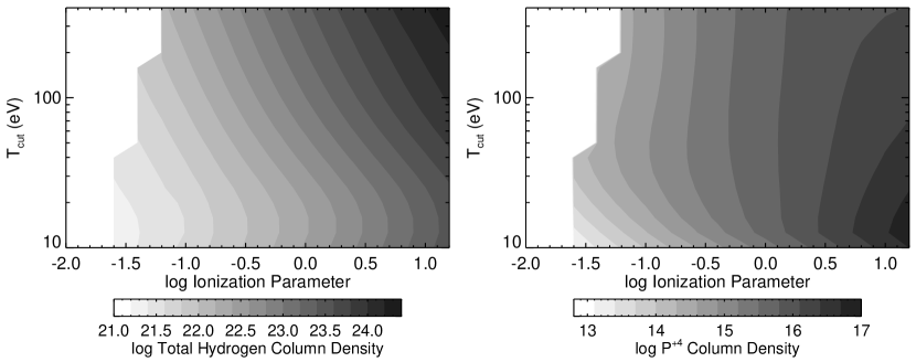
Figure 20: The results depend on the spectral energy distribution. Semi-empirical spectral energy distributions from Casebeer et al. (2006) are parameterized by the cutoff temperature of the UV bump in eV. Left: The total hydrogen column density required to produce the measured He I* column density. Spectral energy dependence is seen, such that softer continua require lower column densities to produce the needed He I* column. Right: The P⁺⁴ column for the simulations shown in the left panel. The fact that the contours are mostly vertical implies that there is little relative spectral energy distribution dependence between P V and He I*.

Almost all of the density discriminators discussed above are predicted to be strongly blended. P IV$\lambda 951$ is obliterated by a combination of C III, N III, and S VI. As we noted previously, S IV is predicted to be highly saturated. Si III* near 1112 is not modeled by Cloudy but may not be present in these data due to the high critical density; recall that high densities are excluded for these data due to the lack of Balmer absorption (§3.1). However, information about C III$\lambda 1176$ may be useful. It is predicted to be present for low ionization parameters, but not for high ionization parameters. It is partially blended with S III$\lambda 1195$, which is very strong at low ionization parameters (Fig. 20), but the higher velocity portion of the trough should be unblended.

As mentioned above, this simulated spectrum is constructed only considering the absorption component responsible for the He I*. There may be both lower and higher ionization absorption components. We know there is a lower-ionization component that is responsible for the Ca II absorption; the simulations shown here, even for the lowest ionization parameters, do not predict any Ca II absorption. But that feature is relatively narrow and has low velocity, so confusion caused by blending would be less of an issue.

3.2.3 Broadband Continuum

If the simulated UV spectrum approximates the real one, then we expect that FBQS J1151$+$3822 should be highly attenuated in the UV simply due to the absorption lines. For example, between 800 and 1600Å, the simulated spectra predict that the observed flux should be about half of the intrinsic flux. With the covering fraction taken into account, the observed flux would be a somewhat higher fraction of the intrinsic flux.

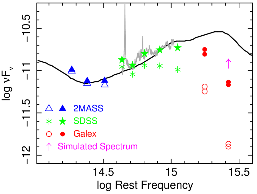
Figure 11: The broadband spectral energy distribution constructed from non-simultaneous photometry data. The solid line is the Richards et al. (2006) spectral energy distribution scaled to the 1 micron break. The open points show the observed data (corrected for Galactic reddening and redshift); the solid points show the observed data dereddened by $E(B-V)=0.1$ and an SMC reddening curve (Pei, 1992). The grey line shows the SDSS spectrum dereddened by the same amount. The arrow shows the flux predicted by the simulated spectra. The fact that the UV data lie below the SED shows that the UV is attenuated by absorption lines as well as intrinsic reddening.

Fig. 11 shows the infrared–UV broad band continuum spectrum constructed from the SDSS, 2MASS and GALEX photometry. It is compared with the SED constructed by Richards et al. (2006) scaled to roughly match the flux at the one-micron dip. It is also compared with the SDSS spectrum of FBQS J1151$+$3822 (reddening corrected; see below). For a redshift of 0.3344, the GALEX FUV band spans $\sim 1000$–1300Å. In this band, the flux from the simulated spectra is predicted to be about about 45% of the intrinsic flux; this is marked by the arrow on Fig. 11. Partial covering would increase the flux; hence the upward-pointing arrow. The observed flux in the FUV GALEX filter (central rest wavelength of 1136Å) is only about 5% of the observed spectrum. So the observed flux is much fainter than can be explained by the simulated absorption alone.

The optical continuum from the SDSS spectrum and also from the photometry (which may not be strongly affected by absorption lines except possibly in the U band) is slightly flat. This could be a consequence of reddening, but is is somewhat difficult to estimate how much reddening is present. We assume that the spectrum would have the same slope as the Richards et al. (2006) SED once the reddening has been removed. We deredden the SDSS spectrum using various values of $E(B-V)$ and an SMC reddening law (Pei, 1992). We find that the maximum reddening that the spectrum can accommodate without becoming much bluer than the composite is $E(B-V)=0.1$. Fig. 9 shows the spectrum and photometry points dereddened by this amount. In this case, the dereddened observed flux in the FUV filter is about 0.23 dex below the Richards et al. (2006) curve, corresponding to $\sim 18$% of the intrinsic flux. So, with reddening taken into account, the FUV flux is still lower than expected from the simulated spectrum. Partial covering would increase the discrepancy. It should be noted that these observations were not simultaneous, and evidence for variability is seen between the two GALEX observations separated by eleven months.

Interestingly, the dereddened SDSS spectrum matches the (Richards et al., 2006) photometry quite well. We use the scaled (Richards et al., 2006) photometry to obtain the intrinsic flux at 2500Å, measuring that to be $8.95\times 10^{-15}\rm\,erg\,cm^{-2}\,s^{-1}$Å^-1. This corresponds to a luminosity density of $6.8\times 10^{30}\rm\,erg\,s^{-1}\,Hz^{-1}$ at 2500Å.

4 Discussion

In this paper, we report the IRTF and MDM observations of FBQS J1151$+$3822, the analysis of those data, and the analysis of the SDSS spectrum. In particular, we analyze the absorption lines from He I* located at 3889Å and 10830Å. We extract the apparent optical depth profile as a function of velocity from the spectra, finding that FBQS J1151$+$3822 is a true BALQSO, with $v_{max}\approx 11,000\rm\,km\,s^{-1}$. We integrate over these optical depth profiles to find the He I* column density. The results for these two lines do not agree, indicating that inhomogeneous covering is present. We also extract an upper limit on the column density of hydrogen in $n=2$. We perform an inhomogeneous absorber analysis of the He I* lines, using partial covering and power law models. We find that the average log column density of the He I* is 14.9. Cloudy modeling, using this mean column density and the upper limit on the hydrogen $n=2$ shows that the ionization parameter must be greater than $\log U=-1.4$, the log density must be less than $\log n=8$, and the log hydrogen column density must be greater than $N_{H}=21.6$. Using the Cloudy models, we produced simulated UV spectra to try to identify lines the could help us better constrain the ionization parameter and density. We found that the ionization parameter could be constrained using a combination of low ionization lines, such as Mg II$\lambda 2800$ or N III$\lambda 990$, which present decreasing optical depth as a function of ionization parameter, and a high ionization line such as P V$\lambda 1118$, which has increasing optical depth as a function of ionization parameter. Density constraints are more difficult; several candidate lines were identified, but because of blending only C III*$\lambda 1176$ seemed potentially useful. Finally, we examine the broad band photometry and show that there is probable evidence for reddening in FBQS J1151$+$3822. However, the dramatic attenuation in the UV band sampled by GALEX is still a factor of $>2.5$ below that explained by the simulated spectrum and the reddening correction.

In this section, we investigate the mass outflow rate and kinetic luminosity inferred. We also discuss plausible acceleration mechanisms. We discuss the potential that He I* has for detecting high-column-density BALQSOs and measuring their outflow properties. Finally, we discuss the future prospects for observing additional He I*$\lambda 10830$ BALQSOs, and the value of constructing a low-redshift BALQSO sample.

4.1 Outflow Rate and Kinetic Luminosity

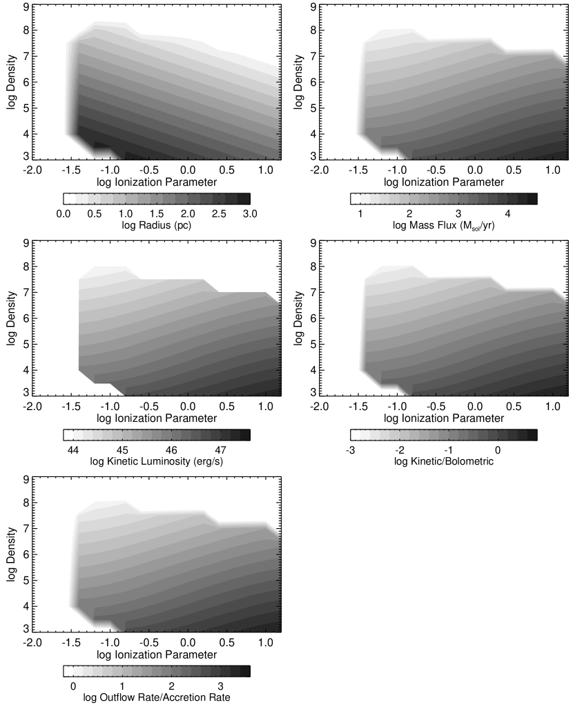
Figure 12: Top left: The absorption-line radius inferred from the Cloudy modeling. Top right: The mass outflow rate. The minimum mass flux allowed by our data is about 10 $M_{\odot}\rm\,yr^{-1}$. Middle left: The kinetic luminosity. Middle right: The ratio of the kinetic luminosity and the bolometric luminosity. Bottom left: The ratio of the outflow rate to the accretion rate.

Using the results presented in §3.1, we can compute physical parameters of the outflow as a function of ionization parameter and density. The combination of the ionization parameter and the density yield the radius of the outflow. These are shown as a function of ionization parameter and density in Fig. 12.

We can compute the mass outflow rate, given by e.g., Dunn et al. (2010)

$$\dot{M}=8\pi\mu m_{p}\Omega RN_{H}v$$

where $\mu=1.4$ is the mean molecular weight, $m_{p}$ is the mass of the proton, $\Omega$ is the global covering fraction, and $v$ is a characteristic velocity. For $v$, we use the column-weighted velocity from the modeling. This value depended slightly (range of $\sim 14$%) on the form of the derivation of the He I*$\lambda 3889$ optical depth, and whether we used a partial covering or powerlaw model. We used a central value of $-5400\rm\,km\,s^{-1}$. The mass outflow rate is also shown in Fig. 12.

The kinetic luminosity is given by e.g., Dunn et al. (2010)

$$\dot{E}_{k}=\frac{\dot{M}v^{2}}{2}=4\pi\mu m_{p}\Omega RN_{H}v^{3}$$

These are also shown in Fig. 12.

We compute the bolometric luminosity by integrating over the Cloudy input flux density scaled to the dereddened flux density (Fig. 11) and using a luminosity distance of 1748.7 Mpc. For some of the higher ionization, higher column-density models, a considerable electron column density is present which, by Thompson scattering, would attenuate the incident flux, making the observed flux smaller. The Cloudy simulations show that this attenuation can be up to $\sim$50%. However, the covering fraction of the electrons is unknown. If the electrons are only present in the gas responsible for the UV absorption, then using a typical value of the covering fraction of 0.3, we find a maximum attenuation of only 15%. On the other hand, the fraction of the source not absorbed by He I* may be transmitted through completely ionized gas, yielding no absorption lines but resulting in attenuation due to Thompson scattering. Given these geometrical complications, we ignore the effects of Thompson scattering. The bolometric luminosity then is $5.3\times 10^{46}\rm\,erg\,s^{-1}$. The log of the ratio of the kinetic luminosity to the bolometric luminosity is shown in Fig. 12.

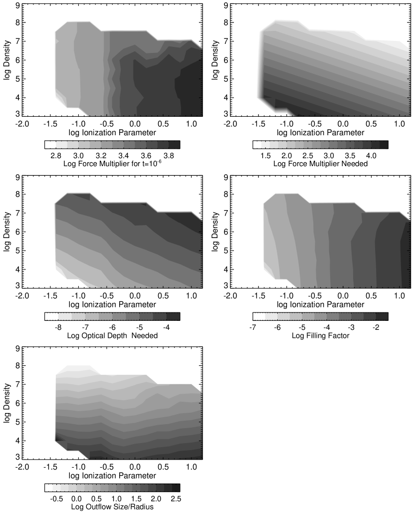
Figure 14: Top left: The line force multiplier estimated from the Cloudy output results for an example value of the equivalent electron optical depth of $10^{-6}$. Top right: The log of the force multiplier needed to attain the terminal velocity of $11,000\rm\,km\,s^{-1}$ observed in FBQS J1151$+$3822. Middle left: The log of the equivalent electron optical depth required to attain the force multiplier needed to accelerate the outflow to the observed terminal velocity, given the force multiplier values computed from the Cloudy results. Middle right: The filling factor needed to accelerate the outflow to the observed terminal velocity. We assume that $dv/dr$ is approximately the terminal velocity divided by the radius where the absorption occurs, obtained from the photoionization modeling results. Bottom left: The ratio of size of the outflow to the absorption radius. Values much larger than zero (i.e., a ratio equal to one) are unphysical.

Assuming an efficiency of 10% of converting matter into radiation, the inferred bolometric luminosity corresponds to a mass accretion rate of 9.3 solar masses per year. The outflow rate is larger than this in every part of the allowed parameter space, ranging from being almost equal at high densities and low ionization parameters, to being more than 1000 times larger at the lowest densities. The log of the ratio of the outflow rate to the accretion rate is also shown in Fig. 14.

How do these results compare with others? Dunn et al. (2010) compile results from partial covering analyses of 8 quasars. Their radii estimates range from 1 pc to 28 kpc. Our possible solutions encompass that range, with the smaller radii being inferred for higher density or higher ionization parameter regions of parameter space. Their mass fluxes range from 0.2 to 590 $M_{\odot}\rm\,yr^{-1}$. Our minimum mass flux is about 10 $M_{\odot}\rm\,yr^{-1}$. Their log kinetic luminosity ranges from 41.1 to 45.7, while our minimum log kinetic luminosity is $\sim 44$, and so is higher than at least half of their sample, and can be very large in the low-density high-ionization region of parameter space. Thus, it appears that FBQS J1151$+$3822 is a relatively powerful BALQSO.

4.2 Acceleration Mechanisms

It is not known how BALQSO winds are accelerated, and several theories have been proposed. An attractive model supposes that the wind is accelerated by the scattering of the photons that create the absorption lines (radiative line driving). This mechanism is also believed to accelerate winds in other objects such as stars and CVs. There is some observational evidence that this mechanism is at work in at least some BALQSOs. The “ghost of Lyman $\alpha$” is one piece of evidence (Arav et al., 1995; Arav, 1996; Korista et al., 1993; North et al., 2006; Cottis et al., 1010). This is observed as a decrease in optical depth near $-5900\rm km\,s^{-1}$. It occurs at this velocity offset because that is where Ly$\alpha$ broad-line region photons are resonantly scattered by N V ions. These extra photons, above the continuum, create additional acceleration causing a decrease in optical depth in velocity space. This feature has not, by any means, been found in all objects, but it has been confirmed in more than a few.

Another piece of evidence is the observed correlation of the maximum velocity of the outflow, $\rm v_{max}$, with the UV luminosity (Laor & Brandt, 2002; Ganguly et al., 2007). More precisely, an upper envelope has been found so that low-luminosity objects have only low values of $\rm v_{max}$, while high luminosity objects have a range of high to low values. Models of radiative acceleration predict that $v_{max}\propto L^{\alpha}$, where the power law index $\alpha$ lies in the range 0.25–0.5 (see Laor & Brandt (2002); Ganguly et al. (2007) for details of these arguments). This correlation argues that radiative acceleration of some kind is generally active in BALQSOs because the correlation is seen in different large samples of objects. Note, though, that the driving force need not necessarily be line driving; acceleration via dust-scattering opacity would also apply (Laor & Brandt, 2002). Note also that this behavior has been seen to be violated in at least one object (WPVS 007; Leighly et al., 2009).

Other mechanisms besides radiative line driving have been suggested for the acceleration of the outflowing gas. Radiative acceleration by dust-scattering opacity has been hypothesized (Scoville & Norman, 1995, e.g.,). This mechanism is promising since dust grains have large opacity. However, the outflow needs to originate beyond the dust sublimation radius, though. For our object, with estimated bolometric luminosity of $5.3\times 10^{46}\rm\,erg\,s^{-1}$ (§4.1), the sublimation radius is estimated to be about 1.2 pc (Scoville & Norman, 1995). As shown in Fig. 12, that radius is spanned by our Cloudy modeling solutions. In addition, we have found evidence for reddening in this object (§3.2.3).

Another model appeals to a magnetocentrifugal wind (e.g., Everett, 2005, and references therein). In this model, gas is attached to large-scale magnetic field lines, and then the rotation of the accretion disk flings the matter away from the disk like beads on a wire. Therefore, in a pure magnetocentrifugal wind, the dynamics of the outflow are divorced from the radiation field. Many people consider a hybrid model, assuming both magnetocentrifugal acceleration and radiative line driving. Finally, thermally-driven winds have been proposed (Krolik & Kriss, 2001), where the wind is essentially evaporated off the inner edge of the torus. This model has been applied principally to warm absorbers rather than BALQSOs.

As an interesting combination of the above, Gallagher & Everett (2007) propose that different models may be appropriate for different regions of the outflow. The X-ray absorbing region may be dominated by magnetocentrifugal acceleration, the UV-absorbing region may be dominated by radiative line driving, and the IR absorbing region may be dominated by dust acceleration.

In this section, we apply several of the radiative-driving models to our results for FBQS J1151$+$3822.

Hamann (1998) presents a derivation of an equation that can be used to determine, in an approximate way, if radiative-line driving is sufficient to accelerate gas of a given column density to a particular terminal velocity. Basically, the equation of motion is solved making the assumption that a fraction of the total luminosity $f_{l}$ is scattered or absorbed by the outflowing gas, as follows:

$$m_{H}N_{H}v\frac{dv}{dr}=\frac{f_{l}L}{4\pi R^{2}c}-\frac{m_{H}N_{H}GM_{BH}}{R^{2}}$$

where $N_{H}$ is the column density of the outflowing gas. To put it another way, the momentum of that fraction of the total radiation is converted to momentum of the wind, mediated naturally by the gravitational attraction of the black hole.

To use this equation, we need to estimate the black hole mass; we do that using standard methods from the SDSS spectrum. We measure a rest frame flux at 5100Å of $2.6\times 10^{-15}\rm\,erg\,s^{-1}\,cm^{-2}$Å^-1 from the dereddened SDSS spectrum shown in Fig. 11. We compute the broad-line-region radius using the regressions found by Bentz et al. (2006) using the flux and a luminosity distance of $1773.7\rm\,Mpc$ appropriate for their (inferred) cosmological parameters of $H_{0}=70\rm\,km\,s^{-1}\,Mpc^{-1}$, $\Omega_{M}=27$ and $\Omega_{\Lambda}=0.73$. That is found to be $\log(R_{BLR})=2.47$ in units of light-days. Finally, we compute the dispersion of the H$\beta$ line profile obtained after subtracting the other fitted components, and referring to Collin et al. (2006), we use a scale factor of 1.5 to obtain a black hole mass of $8.2\times 10^{8}\rm\,M_{\odot}$. For the bolometric luminosity of $5.3\times 10^{46}\rm\,erg\,s^{-1}$, we find that the object is radiating at about half the Eddington luminosity.

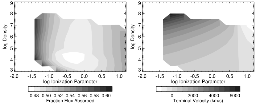
Figure 13: Left: The fraction of the incident continuum absorbed. In principle, the photon momentum from this absorbed light can be converted to momentum of the outflow (Hamann, 1998). Right: The terminal velocities predicted if the fraction of the incident continuum that is absorbed or scattered is converted to momentum of the outflow. Positive velocities denote outflows. Fairly large velocities can be attained; however, they are still lower than the observed terminal velocity of $11,000\rm\,km\,s^{-1}$ observed in FBQS J1151$+$3822.

The fraction of the bolometric luminosity that can be used to accelerate the wind, $f_{l}$, can be estimated as the fraction of the incident continuum that is absorbed. This is easily obtained from the Cloudy output by integrating over the transmitted continuum and dividing the result by the integral over the incident continuum. A difficulty is that for high column densities, the transmitted continuum is attenuated significantly by Thompson scattering. Thompson scattering will not transfer much momentum, so we correct the incident continuum by multiplying it by the Thompson fraction discussed in §4.1. We plot this fraction in Fig. 13. The fraction available is relatively large, equal to or greater than 1/2 over the entire parameter space. It has a broad minimum near $\log U=-0.5$. At lower ionization parameters, more low-ionization species contribute to the optical depth; at high ionization parameters, Compton scattering becomes important.

Next, we can compute the terminal velocity. The bolometric luminosity, obtained above, is estimated to be $5.3\times 10^{46}\rm\,erg\,s^{-1}$. We need a value of the launch radius. Above we computed the radius of the wind from the density and the ionization parameter used in the Cloudy modeling. This is the radius at which the wind has reached its observed velocity and is absorbing the continuum, and so this value would be somewhat larger than the launch radius. Arav & Li (1994) point out that a general characteristic of radiation-driven winds is that most of the acceleration occurs on a length scale comparable to the starting radius. Therefore, for a rough estimate, we use a launch radius that is half the radius of the absorbing wind derived from the Cloudy simulations. The column density is that shown in Fig. 8. The resulting predicted terminal velocity is shown in Fig. 13. A positive velocity (outflow) is attained over most of the parameter space, with higher values attained at higher densities and lower ionization parameters. Higher densities correspond to a smaller launch radius, where the flux is more intense; lower ionization parameters correspond to smaller column densities which are easier to accelerate. Although most of parameter space is characterized by an outflow, the maximum velocity ($\sim 6400\rm\,km\,s^{-1}$) is almost a factor of two below the terminal velocity observed in this object. Still, that we can attain high positive velocities in this object is perhaps not surprising as it is radiating at a large fraction of the Eddington limit.

Could this outflow be a disk wind? It does not seem likely that it is. The disk wind model predicts acceleration to $15,000\rm\,km\,s^{-1}$ at about $10^{17}\rm\,cm$ from the central engine in a $10^{8}\rm\,M_{\odot}$ black hole (Proga et al., 2000). Our photoionization modeling results show that the minimum radius predicted in our parameter space is about 1 parsec for the models with the highest density, out to hundreds of parsecs for lower density models. The distances then range from 10 to thousands of times larger than the disk wind radius.

The above estimate does not take into account the fact that the opacity due to a single line is enhanced by the velocity gradient in an optically-thin outflowing gas. Thus, the momentum transfer for a given column density is greater in an outflowing gas than in a static gas, and higher velocities can be attained. To take this into account, we use the CAK formalism (Castor et al., 1975), originally applied to stellar winds but adapted for use in quasars by e.g., Arav & Li (1994) and Arav et al. (1994).

We compute the force multiplier due to line scattering as a function of the equivalent electron optical depth $t$ in the standard way according to Eq. 2.7 in Arav & Li (1994) using the ionic column densities obtained from our Cloudy simulations, and line opacities obtained from Verner et al. (1994). We ignore bound-free transitions, which will of course also contribute to the acceleration, but probably to a lesser degree than the lines (e.g., Arav et al., 1994, Fig. 2). Fig. 14 shows the log of the force multiplier for an example value of $t=10^{-6}$. For this particular value of $t$ (and noting that the force multiplier has a strong $\sim 1/t$ dependence), we find that the force multiplier is higher for larger ionization parameter. This is because, as discussed in §3.1, the column densities need to be larger at higher ionization parameters to produce the observed He I* column density.

Next, we assume a terminal velocity of $v_{term}=11,000\rm\,km\,s^{-1}$ and a launch radius that is one-half of the radius derived above for the absorbing gas, and solve the equation of motion for the force multiplier and equivalent optical depth $t_{needed}$ required to reach that terminal velocity. The equation of motion that we solve is:

$$v\frac{dv}{dr}=\frac{\sigma_{T}}{1.2m_{H}c}\frac{L}{4\pi r^{2}}M_{L}(U,t)-\frac{GM_{BH}}{r^{2}}$$

where we have assumed that $n_{e}=1.2n_{H}$, i.e., the electron density is approximately 1.2 times the hydrogen density, $L$ is the bolometric luminosity, and $M_{L}(U,t)$ is the force multiplier. The results are shown in Fig. 14. They show almost the same dependence as the radius of the absorbing gas, shown in Fig. 12. This makes sense because the flux decreases rapidly with radius, so the optical depth enhancement due to the velocity gradient has to be higher at larger radii to attain the same terminal velocity. This enhancement is equivalent to a larger value of force multiplier. Likewise, we can solve for the equivalent electron optical depth $t$ needed to attain the observed terminal velocity. That is also shown in Fig. 14. The equivalent electron optical depth $t$ is smaller for larger values of the radius.

The equivalent electron optical depth scale is defined as

$$t=\sigma_{T}\epsilon n_{e}v_{th}\left(\frac{dv}{dr}\right)^{-1}$$

where $\epsilon$ is the filling factor in the wind, and $v_{th}$ is the thermal velocity of the gas. We assume a temperature of $10^{4}\rm\,K$, appropriate for a photoionized gas, and we again assume that the electron density is $1.2n_{H}$. We make the zeroth-order assumption that $dv/dr$ is approximately equal to the terminal velocity divided by the radius where the absorption occurs. Then, we can solve for the filling factor $\epsilon$. That is also shown in Fig. 14.

The filling factor $\epsilon$ can be used to estimate the dimensions of the outflow. For a continuous flow, the length scale $l$ would be $N_{H}/n_{H}$. For a flow consisting of small clouds with filling factor $\epsilon$, the length scale is increased by $1/\epsilon$, i.e., $N_{H}/\epsilon n_{H}$. For the outflow to be physical, the length scale of the outflow must be less than the radius where the absorption occurs; otherwise, there would not be sufficient length to accelerate the outflow to the observed terminal velocity. Working through the approximations given above, we find:

$$\frac{l}{R_{abs}}=\frac{1.2\sigma_{T}N_{H}v_{th}}{t_{needed}v_{term}}.$$

This equation shows that larger column densities require larger region sizes to accelerate all the gas to the terminal velocity. The terminal velocity appears on the bottom of the equation as it was originally part of $dv/dr$, the differential expansion rate. The region size has to be larger for smaller differential expansion rates in order to attain the same terminal velocity.

The log of the ratio of the region size to the radius where the absorption occurs is shown in Fig. 14. This shows that at densities lower than $\sim 10^{7}\rm\,cm^{-3}$, the flow is unphysical since the region size is larger than the absorption radius. This happens because low density flows occur at larger radii, and at a large radius the flux is low, so a large equivalent electron optical depth scale is needed to counteract the low flux and accelerate the flow to the observed terminal velocity. The equivalent electron optical depth scale is linearly dependent on $\epsilon$.

This argument, based on the flow dynamics, provides strong constraints on the physical parameters of the outflow, excluding most of the previously allowed parameter space. Examining Fig. 8 and Fig. 12 and considering areas of parameter space where the region size is smaller or equal to the radius size ($l/R_{abs}\leq 1$), we find that the log of the total hydrogen column density is constrained to be between 21.7 and 22.9, the radius is between 2 and 12 parsecs, the mass flux is between 11 and 54 solar masses per year, the kinetic luminosity is between 1 and 5$\times 10^{44}\rm\,erg\,s^{-1}$, and the kinetic luminosity is between 0.2 and 0.9% of the bolometric luminosity. If we now compare with previous results from Dunn et al. (2010), we find that FBQS J1151$+$3822 has an absorbing region relatively close to the central engine, a higher than average column density, a relatively high kinetic luminosity, but a relatively low mass outflow rate.

It is also interesting to note that the allowed region lies in the area where we expect C III*$\lambda 1176$ to be a useful density diagnostic. We would also expect P V to be weak in the UV spectrum as the ionization parameter is now constrained to be between $-1.4$ and $0.2$ (Fig. 10; middle panel).

This analysis assumes that radiative line driving is the acceleration mechanism operating in this BALQSO; however, that is the favored acceleration mechanism for the UV absorbing gas. At any rate, it implies that radiative line driving is feasible for higher densities in our parameter space. Lower densities would require an additional acceleration mechanism, perhaps hydromagnetic. In addition, we have assumed that the flow is radial. It may be simply crossing our line of sight; in that case, the terminal velocity would be larger than the observed $11,000\rm\,km\,s^{-1}$.

4.3 Size of the Absorbers

Following Hamann et al. (2010), we can compute the size of the absorbers. Reviewing their argument, since partial covering is significant, the upper limit on the size of the individual absorbing structure is the size of the emitting region. This is an upper limit since the absorbers can be smaller, and there can be many of them.

We compute the size of the emission region using classical relations from accretion disk theory, namely, for a sum-of-blackbodies accretion disk,

$$T_{disk}=\big{(}\frac{3GM\dot{M}}{8\pi\sigma R^{3}}\big{)}^{1/4}.$$

We use the black hole mass and accretion rate derived in §4.2, namely $M=8.2\times 10^{8}M_{\odot}$ and $\dot{M}=9.3\,\rm M_{\odot}\,yr^{-1}$. This equation yields a temperature that decreases with radius as $R^{-3/4}$. It has been argued that this radial dependence is too steep (e.g., (Gaskell, 2008), who suggests that the index should be 0.57) yet may be acceptable for the estimations made here. Using this equation, we find that the 3888Å and 10830Å are emitted at 0.011 and 0.045 pc, respectively. Thus, the 10830Å emission region is a factor of 3.9 times larger than the 3888Å emission region; for a flatter temperature dependence of $-0.58$, that difference increases to a factor of 5.8. These sizes are comparable to those inferred by Hamann et al. (2010), despite the fact they are examining far UV lines. The reason for this coincidence is that the black hole mass in their object is much larger.

These numbers become more interested when compared with the much smaller emission region size expected at for 1121Å, where P V absorption should be seen in the continuum. For FBQS J1151$+$3822 that is $0.0022\rm\,pc$, a factor of 21 times smaller than the 10830Å emission region size (and a factor of 50 times smaller for the flatter radial temperature dependence). So, if partial covering in P V were observed in FBQS J1151$+$3822, it would imply that a swarm of at least 20–50 very small clouds cover the 10830Å emitting region.

These numbers become even more extreme when considering the low black hole mass BALQSO WPVS 007 (Leighly et al., 2009). That object has a black hole mass of $4.1\times 10^{6}\rm\,M_{\odot}$ and an accretion rate between 0.0086 and 0.0114 solar masses per year. Yet, it also shows evidence for partial covering in P V. Following the analysis above, we obtain a continuum emission region for 1121Å of 3.6–4.8$\times 10^{-5}\rm pc$.

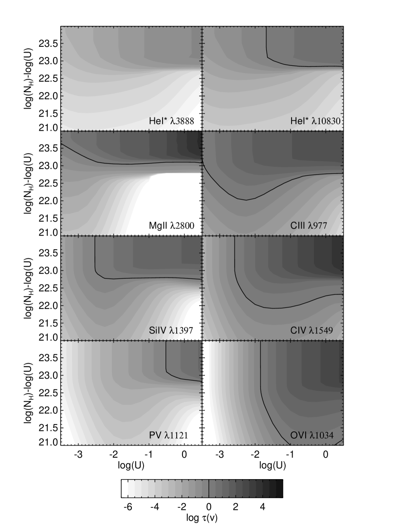
Figure 15: Contours of $\log\tau(v)$ for a selection of lines as a function of ionization parameter and $\log(N_{H})-\log(U)$. We assumed a square absorption profile with velocity width of $10,000\rm\,km\,s^{-1}$. Lower velocity widths would yield higher opacities for any combination of parameters. $\tau(v)=1$ is shown by a contour line to guide the eye. These contours show that resonance lines such as C III and O VI are predicted to be saturated at relatively low column densities, while the high-column-density diagnostic lines including P V, He I*$\lambda 3889$, He I*$\lambda 10830$ remain optically thin until high column densities are attained.

A comparison of the covering fractions of He I* and P V in the same object could be interesting due to the large differences in size of the emitting region (a factor of 20–50, depending on the radial dependence of the temperature). Note that the covering fractions of these lines can be directly compared because the gas presents the same optical depth in these lines (Fig. 15); as discussed by Hamann et al. (2001), lines that have higher optical depths may have naturally higher covering fractions. It is possible that the swarm of small clouds may completely cover the 1121Å emitting region, but not cover the entire 10830Å emitting region. If this were the case, the covering fraction would be different.

4.4 He I* as a High-Column-Density Diagnostic

4.4.1 Comparison with Other Lines

High-column-density outflows are of great interest in BALQSOs. For radiative acceleration models, the force multiplier is predicted generally to decline with column density (e.g., Arav & Li, 1994). So high-column flows place the most stringent constraints on radiative acceleration models. In addition, the kinetic luminosity depends linearly on the column density, so, depending on the velocity and radius, these outflows may have the largest kinetic luminosities, thus placing the most stringent constraints in general on outflow-acceleration models.

The study of BALQSOs underwent a paradigm shift about 15 years ago. Previously, it was thought that the absorber completely covered the continuum, and column densities could be measured directly from the troughs. But the observation of strong P V in some objects was puzzling, given that the solar abundance of phosphorus is about 765 times lower than that of carbon. This conundrum was resolved with the realization that the column densities were much larger than previously thought, but the troughs are not black because the absorber only partially covers the continuum source (Hamann, 1998).

The low abundance of phosphorus means that P V lines will be present only when the column densities are high. Thus, P V is a good probe of high-column outflows. But there is a practical problem with using P V to detect high-column outflows in general: the resonance lines are in the far UV (at 1118 and 1128Å) and shortward of Ly$\alpha$. So low-redshift objects must be observed from space, while in high-redshift objects, when P V is shifted in to the optical bandpass (for redshifts larger than $\sim 2$), P V can be obscured by Ly$\alpha$ forest absorption.

We propose that He I* is an equally effective probe of high column densities in BALQSOs. We discuss the situation analytically first, and then investigate using simulations.

As shown in Savage & Sembach (1991), the optical depth is a function of $\lambda f_{ik}N_{ion}$, where $\lambda$ and $f_{ik}$ are the wavelength and the the oscillator strength of the transition, respectively, and $N_{ion}$ is the column density of the relevant ion. For P V, $\lambda f_{ik}$ is 752 (for both of the resonance transitions for this doublet). For He I*$\lambda 3889$, the product is 251, while for He I*$\lambda 10830$, the product is 5842.

For an analytic estimation, the relevant metric is the $\lambda f_{ik}$ times the fraction of the ion or metastable state relative to hydrogen. The lower the value, the higher the column density can be before the line is saturated.

What is the ratio of P⁺⁴ to hydrogen, approximately? For solar abundances, there is one phosphorus atom for every 312,536 hydrogen atoms. From Hamann (1997) we see the fraction of phosphorus ionized three times is no larger than about 0.5–0.6. Assuming 0.5, we then estimate the abundance of $P^{+4}$ to be $1.6\times 10^{-7}$. Then the $\lambda f_{ik}N_{ion}$ value for P V is $1.2\times 10^{-4}$.

What is the ratio of He I* to hydrogen, approximately? For solar abundances, the helium abundance is 0.1. The metastable level is populated by recombination of He⁺. As discussed by Clegg (1987) and Clegg & Harrington (1989), it is depopulated principally by collisions. Clegg (1987) give an empirical formula for the ratio of helium in the metastable state relative to the number of He⁺

$$\frac{N(2^{3}S)}{N(He^{+})}=\frac{5.79\times 10^{-6}t_{e}^{1.18}}{1+3110t_{e}^{-0.51}N_{e}^{-1}}$$

where $t_{e}$ is the electron temperature in units of $10^{4}\rm\,K$ and $N_{e}$ is the electron density in $\rm\,cm^{-3}$. This function shows that the number of helium in the metastable state is an approximately constant fraction of the number of once-ionized helium.

In an ionized gas slab, only a fraction of helium will be He⁺. As long as the slab is not too thick (i.e., optically thin to the hydrogen continuum), the helium will be split between once and twice ionized atoms. Given that quasar photon continua fall steeply, we can assume that the majority of the helium will be He⁺. Thus, the abundance of metastable helium is approximately $5.8\times 10^{-7}$. Then $\lambda f_{ik}N_{ion}$ is $1.5\times 10^{-4}$ for He I*$\lambda 3889$ and $3.4\times 10^{-3}$ for He I*$\lambda 10830$. Recalling that the $\lambda f_{ik}N_{ion}$ value for P V is $1.2\times 10^{-4}$, we see that He I*$\lambda 3889$ component is equally sensitive as P V, while He I*$\lambda 10830$ is a bit less sensitive. In contrast, a similar estimation for C IV$\lambda 1549$ (for an assumed fraction of C⁺³ of 0.65) is $7.0\times 10^{-2}$. So, for example, C IV will become saturated at column densities a factor of twenty lower than He I*$\lambda 10830$, and a factor of $\sim 470$ lower than He I*$\lambda 3889$.

The analytical analysis is limited because the fraction of these ions in a slab depends on the ionization parameter and column density, as well as the abundances. So, we use the simulations discussed in §3.1 to investigate the sensitivity of these absorption lines to high columns further. As discussed in §3.1, we assume the Cloudy AGN Kirk continuum, solar abundances, and $\log(n)=5$. Since all the transitions discussed here are resonance transitions, we expect negligible dependence on density . We extract ionic column densities as a function of ionization parameter and $\log N_{H}-\log U$ from the Cloudy model results. Contours of $\log\tau(v)=\log(2.654\times 10^{-15}\lambda f_{ik}N_{ion})-\log(10,000)$ are show in Fig. 15. We divide by 10,000$\rm\,km\,s^{-1}$ to approximate the optical depth of a square line profile with a width of 10,000$\rm\,km\,s^{-1}$ , consistent with the approximate width of the line observed in FBQS J1151$+$3822. A smaller velocity width would yield a larger optical depth for any combination of parameters.

These contour plots show that resonance-line absorption from abundant ions, such as O VI and C IV, are saturated at relatively low column densities. But lines such as P V and He I*$\lambda 3889$, and to a slightly lesser extent, He I*$\lambda 10830$, remain optically thin over a wide range of parameter space.

These figures also show that the metal lines experience greater ionization parameter dependence than the He I* lines. That is, for example, Si IV optical depth is greater for any value of $\log N_{H}-\log U$ at $\log U\sim-2.2$ than for other values of ionization parameter. This is of course due to the fact that at $\log U\sim-2.2$, a greater fraction of silicon is Si⁺³ than other ionization states, while at lower and higher values of $\log U$, there are relatively fewer Si⁺³ ions. Metastable He I is more monotonic; for a fixed radiation-bounded slab depth, the number of metastable helium ions increases as the depth of the helium ionization front increases.

4.4.2 Sensitivity Examined Using Simulated Spectra

As discussed above, He I* is a valuable probe of high column density in quasars. Moreover, using both the He I*$\lambda 3889$ and He I*$\lambda 10830$ lines, we can solve for the true column density and covering fraction. In this section, we discuss the range of columns that can be probed using He I*, and we discuss the prospects of identifying low-reshift BALQSOs using He I*.

Each quasar absorption line is sensitive to a certain range of column density. If the column is too low, the absorption line will not be distinguishable from the continuum. If the column is too high, the absorption line will be saturated. Obviously, the sensitivity will depend on the properties of the transition, through the oscillator strength, and it will depend on the abundance of the ion. But it will also depend on the properties of the outflow; in particular, it will depend on the the range of velocity over which the line is spread, $\Delta v$. A low column density is detectable in a narrow line, where $\Delta v$ is small, while absorption spread over a large range of velocity would be indistinguishable from the continuum. The sensitivity depends on the data properties, i.e., signal-to-noise ratio, obviously, with this factor being more important for weak lines. In addition, in some cases, there is systematic uncertainty, such as the uncertainty in defining the continuum.

We explore the sensitivity of the He I* lines using simulations. We use the optical depth profile as a function of velocity obtained from the infrared spectrum. Furthermore, we use this for both lines, that is, we ignore velocity dependence of the optical depth and covering fraction. We smooth the profile slightly using the function mentioned in §2.1. We investigate the region around the 3889Å and 10830Å lines in velocity space. We add gaussian noise to the initial ratio of observed to continuum (equal to 1) so that the resulting signal-to-noise ratio is 150. Clearly, there will be sensitivity dependence on the signal-to-noise ratio, but since we are more interested in the characteristics of the lines, we do not explore that dependence here. We investigate log He I* column densities between 14.0 and 17.0. As discussed above, this corresponds to approximate log hydrogen column densities of 20.25–23.25. We emphasize again that the results depend on the absorption profile assumed here to have $\Delta v\approx 11,000\rm\,km\,s^{-1}$. We also investigate a range of covering fractions between 0.1 and 0.9. For each input column density of He I*, we scale the optical depth profile appropriately to produce the desired column density. Then, for each input covering fraction, and using equations 3 and 4 from Sabra & Hamann (2005), we simulate the observed ratio of absorbed to continuum spectra for both the 3889Å region and the 10830Å region. Finally, we fit the two resulting simulated ratios with the partial covering model using the technique discussed in §2.8. For each combination of parameters, we run 10 simulations and plot the mean.

As discussed qualitatively above, metastable helium is a valuable probe of high column densities because helium in this state is relatively rare in the gas. In that way, metastable helium absorption is similar to P⁺⁴ absorption. But the He I*$\lambda 10830$ and He I*$\lambda 3889$ lines have another unique property: the high $\lambda f_{ik}$ ratio of 23.3. In contrast, the P V$\lambda\lambda 1118,1128$ lines, like other lithium-like ions, have a $\lambda f_{ik}$ ratio of 2. What effect does the $\lambda f_{ik}$ ratio have on the sensitivity? To explore this question, we do another set of simulations in which $\lambda f_{ik}$ for the 3889Å line is a factor of two lower than $\lambda f_{ik}$ for the 10830Å line, instead of the normal case where the ratio is 23.3.

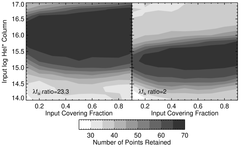
Figure 16: There are 69 points in the IRTF velocity profile. The fitting software excludes unphysical points where $R_{3889}>R_{10830}>R_{3889}^{23.3}$ is not obeyed. Contours show the number of points retained in the fitting.

The results are shown in Fig. 16–19. We plot the measured properties as a function of the input parameters. We first plot the number of points retained in Fig. 16. The optical depth profile had 69 points, and as noted in §2.8, the software removes unphysical points where $R_{3889}>R_{10830}>R_{3889}^{23.3}$ is not obeyed. We see that the number of points retained is lower for the lowest and highest column densities. This makes sense for the lowest column densities, since in that case, the optical depth of both lines is low, and it is more likely that a fluctuation due to noise will cause a point to become unphysical. At highest column densities, the lines become saturated, and the ratio of the observed to continuum looks the same for both lines. Again, in this case, is it likely that a fluctuation due to noise will cause a point to become unphysical. The number of points retained drops less rapidly for $\lambda f_{ik}=23.3$ as the low value of the oscillator strength of the 3889Å line means that it is not saturated until the column density becomes very high.

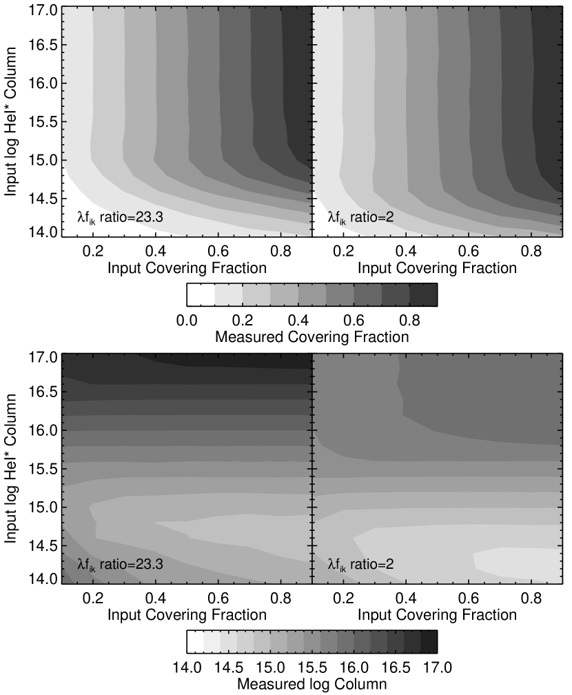
Figure 17: The measured covering fraction (top) and column density (bottom) as a function of the input covering fraction and column.

Next, we plot the measured covering fraction and column density from the partial covering model in Fig. 17. The measured covering fraction and column density is consistent with the input for intermediate $\log$ He I* column densities for both sets of simulations. For lower column densities, the measured covering fraction is consistently low, while the column density is consistently high. At lower column densities, the weaker line becomes indistinguishable from the continuum, and unphysical points are dropped. Points are deemed physical if there is a downward fluctuation in the 10830Å component, and an upward fluctuation in 3889Å. This situation looks the same as a higher column and a lower covering fraction. For the highest column densities, the measured column is consistent with the input for the $\lambda f_{ik}$ ratio $=23.3$ case, while it is consistently underestimated for the $\lambda f_{ik}$ ratio $=2$ case. This is because at high column densities, both lines become saturated when $\lambda f_{ik}$ ratio$=2$.

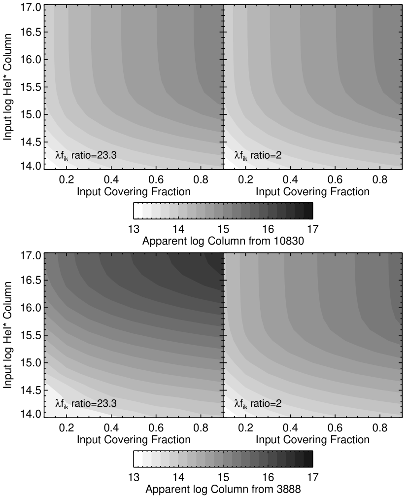
Figure 18: Apparent column densities measured from the 10830Å profile (top) and from the 3889Å profile (bottom).

How would we fare if we had only one of the two He I* lines? Fig. 18 shows the apparent column densities measured from the 10830Å line and the 3889Å lines separately. We find that the column density is uniformly less than the observed, as expected. The discrepancy is less for high covering fractions; the presence of significant partial covering, i.e., small values of the covering fraction, makes the optical depth look too low. There is also a saturation of column at high column densities for a given covering fraction. This is due to saturation of the lines. The 3889Å line (with $\lambda f_{ik}$ ratio $=23.3$) performs the best at high column densities because the low oscillator strength of this line prevents it from becoming saturated. The apparent column density is lower than the input for small values of the covering fraction, for the same reason as above: low values of the covering fraction make the apparent optical depth low.

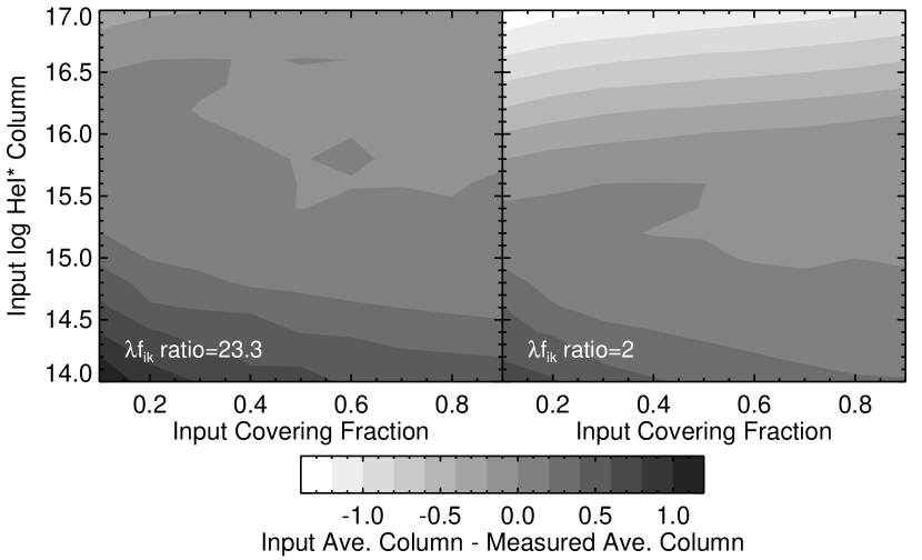
Figure 19: Difference between the log of the input average column and the measured average column. Values around zero show the regions of parameter space where the mean column (used in photoionization and dynamical models) is best reproduced.

Finally, in Fig. 19 we plot the difference between the log of the measured average column density and the log of the input average column density. Recall that the average column density for the partial covering model is the product of the covering fraction and the column density. This is the relevant parameter for the photoionization and dynamical modeling. For smaller column densities, the accuracy is better for larger covering fractions; for smaller covering fractions, the observed column is overestimated but by less than an order of magnitude. More importantly, this plot shows that the average column is accurately reproduced for input log He I* column densities larger than $\sim 15$ when the $\lambda f_{ik}$ ratio $=23.3$. For a $\lambda f_{ik}$ ratio $=2$, both lines become saturated at high column densities, and the input column density is estimated to be too low by an order of magnitude.

In summary, these simulations show that while there is some bias in measuring parameters at low column density (which is not surprising since as the lines become indistinguishable from the continuum), the large $\lambda f_{ik}$ ratio $=23.3$ for He I$\lambda 10830$ and He I$\lambda 3889$ makes it superior for measuring high column densities. Basically, the large ratio gives these lines an increased dynamic range for measuring high column densities. An important point, though, is that the values in these simulations apply for the optical depth profile derived for He I$\lambda f_{ik}$ for FBQS J1151$+$3822; the columns measurable will vary depending on the distribution of column over velocity, $dN/dv$.

4.5 Are There More He I*$\lambda 10830$ BALQSOs?

In this paper, we report the discovery of the first He I*$\lambda 10830$ broad absorption line quasar. Are there any more of them? In principle, there should be. He I* is a high-ionization ion that appears in the He⁺ region of the outflow, coincident with C⁺³ and Si⁺³. If the column densities are generally large, then any high-ionization outflow should have He I*$\lambda 10830$.

Actually, we have already found some. An observing run in April 2010 using SPEX on the IRTF has netted four additional objects. In addition, observations using Lucifer on the LBT has yielded two more (Leighly et al. in prep.). But not all BALQSOs have He I*$\lambda 10830$; we observed several well-known low-redshift BALQSOs using SpeX on the IRTF and found that they do not have significant He I*$\lambda 10830$ absorption. These are bright objects for the IRTF so the limits on He I*$\lambda 10830$ will provide interesting upper limits on the column density in these objects (Leighly et al. in prep.).

How can we find more candidates? The Sloan Digital Sky Survey spectra provide a useful starting place. If we can identify He I*$\lambda 3889$ in SDSS spectra, then, because of the large $\lambda f_{ik}$ ratio, He I*$\lambda 10830$ will certainly be seen. How can we identify objects with He I*$\lambda 3889$? As discussed in §2.4, it can be difficult as it is generally a weak line that can be confused with strong Fe II emission. One way is to look at objects that have both Mg II and He I*$\lambda 3889$ in the bandpass. An informal examination of a low-redshift subsample of BALQSOs cataloged by (Gibson et al., 2009) shows that $\sim 1/3$ have something at 3889Å that may correspond to the Mg II absorption.

Identifying He I* BALQSOs using both Mg II and the 3889Å component limits us to Lo-BALs. How can we identify high-ionization BALQSOs? One way is to look for objects that do have He I*$\lambda 3889$ but don’t have Mg II. Another possibility is to look at the broad band photometry. The FBQS J1151$+$3822 photometry shown in Fig. 11 is rather distinctive, as the decline in the UV is too steep to be explained by reddening. Depending on the redshift, the usefulness of this technique will depend on the availability of GALEX photometry.

Observing He I*$\lambda 10830$ limits us to low redshift objects. If we observe He I*$\lambda 3889$ in the optical band, we will observe the 10830 component in the 0.8–$2.4\mu$ short-wavelength band; then, we are limited to objects with redshifts less than 1.2. But these nearby objects may be quite interesting. Only a handful of low-redshift BALQSOs are known (e.g., Sulentic et al., 2006). Many of these were discovered serendipitously; for example, they were observed because they are PG quasars, or because they have weak [O III] in their optical spectra (Turnshek et al., 1997). These low-redshift objects have lower luminosities than the SDSS and LBQS BALQSOs (e.g., Fig. 7 in Ganguly et al., 2007), and so they define the low-$v_{max}$ end of the correlation between $v_{max}$ and luminosity. That region of the plot is rather sparsely populated, but it may be important in our understanding of outflows in AGN as it bridges the very low velocity outflows seen in Seyfert galaxies (e.g., Crenshaw et al., 2003) and the high velocity BALQSOs beyond $z>1.5$. FBQS J1151$+$3822 is a luminous object; for Ganguly et al. (2007)’s cosmology, the dereddened 3000Å $\log\lambda L_{\lambda}$ is 45.9 (without the reddening correction, $\log\lambda L_{\lambda}=45.7$; Fig. 11). From Ganguly et al. (2007) we see that lower luminosity objects of interest should have $\log\lambda L_{\lambda}<\sim 45.1$, or greater than 2 magnitudes fainter than FBQS J1151$+$3822. But FBQS J1151$+$3822 is a relatively bright object for SDSS, with an observed g magnitude of 15.8. The DR7 SDSS Quasar Catalog (Schneider et al., 2010) has 37,430 quasars with redshift smaller than 1.2, and the distribution of g-magnitude peaks at 19, while there are only 35 quasars brighter than FBQS J1151$+$3822. Thus, it seems quite reasonable that an interesting low-redshift low-luminosity sample could be defined and studied.

5 Summary & Conclusions

The principal results and findings of this paper are as follows.

• We report the first short wavelength (0.8–2.4$\mu$) infrared spectroscopic observation of FBQS J1151$+$3822 using SpeX on the IRTF, as well as a new optical spectroscopic observation of FBQS J1151$+$3822 using CCDS on the 2.4 meter Hiltner telescope at MDM observatory. In addition, we analyzed the SDSS spetrum. We discovered broad He I* absorption lines, both in the 3889Å transition and, for the first time in a quasar, in the 10830Å transition. The terminal velocity $v_{max}$ is $11,000\,\rm km\,s^{-1}$, indicating that FBQS J1151$+$3822 is a broad absorption line quasar.

• We extracted the apparent optical depths for the absorption lines. The procedure was straightforward for the 10830Å line because the IR continuum is fairly simple. But for the 3889Å line, this procedure was complicated by strong Fe II emission, so a template-fitting method had to be used. An upper limit on Balmer absorption was extracted from the SDSS spectrum.

• The He I* column densities were first estimated by integrating directly over the optical depth profiles. The estimate based on the 3889Å line ($\log N_{HeI*}\sim 14.85$) was substantially higher than the one based on the 10830Å line ($\sim 14.3$). This result implies that the absorber does not fully cover the source. Since the two transitions have the same lower (metastable) level, we can solve two-parameter inhomogeneous covering models as a function of velocity. We use a pure partial covering model and a power law model. Both models give the same average log He I* column of 14.9. The hydrogen $n=2$ limit depends on the details of the population of the $2p$ and the $2s$ states; assuming that the $2s$ metastable state was solely populated yielded an upper limit of log hydrogen $n=2$ column of 13.5.

• Cloudy modeling was used to constrain the range of parameter space permitted by the measurements. The ionization parameter $\log U$ must be greater than or equal to $-1.4$ in order to produce sufficient He I*. A log density less than $\sim 8$ was required, or too much Balmer absorption was predicted. The log hydrogen column density was constrained to be greater or equal to 21.6. Comparison with other objects showed that FBQS J1151$+$3822 is a relatively high-ionization, high-column-density BALQSO.

• The Cloudy simulations were used to see if UV spectra would be able to constrain parameters further. It was found that ionization parameter would be reasonably easily constrained through observation of low ionization lines such as Mg II and N III, which decrease in optical depth as the ionization parameter increases, and observation of the high ionization line P V, which increases in optical depth as the ionization parameter increases. Several density diagnostic lines were examined; all were predicted to be too blended to be useful except for the high-velocity side of C III*$\lambda 1176$.

• The broad band photometry was examined. The observed decrease in the UV was too steep to be solely caused by reddening. Attenuation is expected also because of the absorption lines predicted in the UV. However, a combination of correction for modest reddening ($E(B-V)=0.1$ for an SMC reddening curve) and attenuation due to predicted high-ionization absorption lines left the observed UV still a factor of $\sim 2.5$ too low.

• The mass outflow rate, kinetic luminosity and ratio of kinetic to bolometric luminosity were estimated. The range was large over allowed parameter space but generally the minimum values were higher than those estimated in other objects.

• Acceleration mechanisms were examined. A force-multiplier analysis was done using the Cloudy results. It was found for this luminous object, radiating at about 1/2 the Eddington luminosity, the terminal velocity $v_{max}$ could be easily achieved. Furthermore, a comparison of the size scale of the outflow with the radius of the outflow constrained the log of the density to be greater than $\sim 7$. This strongly constrained parameter space, yielding an acceptable range log hydrogen column densities of 21.7–22.9, radii between 2–12 parsecs, mass outflow rates between 11 and 54 solar masses per year, ratio of outflow to inflow rates between 1.2 and 5.8, kinetic luminosity between 1 and $5\times 10^{44}\rm\,erg\,s^{-1}$, and kinetic luminosity between 0.2 and 0.9% of the bolometric luminosity. Compared with other objects, FBQS J1151$+$3822 has a relatively powerful outflow originating relatively close to the central engine.

• We examine the potential for using the He I* absorption lines to detect and measure the properties of high-column-density BALQSOs. Objects with high column densities may require the highest kinetic energies and so may be important for testing models. We demonstrate that many prominent BAL lines become saturated at high column densities. We show that He I*$\lambda 10830$ compares favorably with P V, a widely used probe of high column densities, while He I*$\lambda 3889$, because of its low oscillator strength, is even more sensitive. We use simulated spectra to see how well we can reproduce input covering fractions and column densities using a partial covering model. We find that the high $\lambda f_{ik}$ ratio of 23.3 makes the He I* lines more sensitive to a wider range of column density than lines with a $\lambda f_{ik}$ ratio equal to 2 (like P V).

• We briefly discussed the prospects of finding other He I*$\lambda 10830$ BALQSOs. We have in fact already collected data on six additional objects; furthermore, we have discovered that several well-known, bright low-redshift BALQSOs have no He I*$\lambda 10830$ absorption, a fact that will place upper limits on the column densities in those objects. We discussed the utility of observing a sample of low-redshift BALQSOs identified via He I* absorption. Such objects may be valuable for understanding the relationship between luminosity and terminal velocity $v_{max}$ by allowing definition of a lower luminosity sample in a region currently sparsely populated.

Appendix A Spectral Energy Distribution Dependence

The incident spectral energy distribution influences the results. We examine this using an updated version of the semi-empirical spectral energy distributions developed in Casebeer et al. (2006). They are parameterized by the cutoff temperature of the UV bump measured in electron volts. The Korista et al. (1997) AGN Kirk continuum is similar to a spectral energy distribution with $T_{cut}=80\rm\,eV$. Because the He I* does not have significant density dependence, we investigate the behavior as a function of ionization parameter and $T_{cut}$ for a single value of the density $\log n=5.5$.

We first investigate the total hydrogen column density needed to attain the required He I* column. The results are shown in Fig. 20. We find that softer spectral energy distributions (i.e., lower values of $T_{cut}$) require lower values of the hydrogen column density for a particular ionization parameter, while harder SEDs require larger values of the hydrogen column density. This makes sense because helium ionization front occurs at a smaller depth when the SED is soft, and at a larger depth when the SED is hard. Thus, the location of recombining He⁺ shifts in the slab.

We also investigate the column density of P⁺⁴ as a function of ionization parameter and spectral energy distribution (Fig. 20). As discussed in Leighly et al. (2009), the P⁺⁴ zone also occurs deeper in the slab when the spectral energy distribution is hard than when it is soft. But here we see it is almost constant for a given ionization parameter (for higher values of the ionization parameter where P V absorption would be detectable). This simply shows that the depth of the P⁺⁴ region shifts in the gas in the same way as the He⁺ region as a function of SED. Thus, there appears to be little relative dependence on spectral energy distribution between these two lines.

Appendix B Metallicity Dependence

The metallicity of the gas will also influence the results. We briefly investigate the effect of metallicity by running a grid of models with the Korista et al. (1997) AGN kirk continuum and a metallicity five times that of solar ($Z=5$). As discussed in Hamann et al. (2002, Table 2), this means that each metal element is five times more prevalent with respect to hydrogen than at solar abundance, with the exception of nitrogen, which because of the secondary production process is 25 times more abundant than at solar metallicity. In addition, helium is enhanced by a factor of 1.29.

Notable differences were seen between the $Z=5$ metallicity results and the solar metallicity results presented in §3.1. First, there is a difference in the hydrogen column density required to produce the observed metastable helium column density, namely, the allowable solutions extend to lower ionization parameters, down to $\log U=-1.8$ versus $\log U=-1.4$ for solar metallicity. At these lower ionization parameters, we expect lower ionization species to be more prominent; that could potentially be recognized in the UV spectrum (see below; §3.2.2).

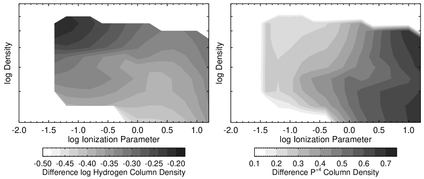
Figure 21: The results depend on the metallicity of the gas. We show the difference in the log of the column densities for the $Z=5$ case and the solar metallicity case discussed in §3.1. Left: The difference in the log column density of the hydrogen column necessary to produce a sufficient metastable neutral helium column. Right: The difference in log column density of P⁺⁴.

One might imagine that the column densities from the higher metallicity grid might differ from the solar metallicity grid by a constant factor reflecting the abundance differences. However, the presence of enhanced metals changes the cooling in the gas (e.g., Hamann et al., 2002), and so the results are not so simple. We show the difference in the log column between the $Z=5$ and the $Z=1$ results in Fig. 21, both for the total hydrogen column and the P⁺⁴ column density. We include only regions of parameter space were both solutions exist.

For the total hydrogen density, we see that the difference in the log of the column density is negative in all cases. This means that the column required is lower in the $Z=5$ case, as expected. As mentioned above, in the $Z=5$ experiment, the abundance of helium is enhanced by a factor of 1.29. This corresponds to a difference in log of 0.11. We observe a much larger range of differences, with the largest difference up to almost $-0.5$ for lower densities. We suspect this is a consequence of enhanced cooling at low densities due to the higher metallicity. As mentioned above, the metastable state is populated by recombination from He⁺¹ and depopulated chiefly by collisions (Clegg, 1987; Clegg & Harrington, 1989). When the temperature is lower, a larger fraction remains in the metastable state. So a smaller total hydrogen column is necessary to attain the required column of He I*. The effect is enhanced at low densities where the gas generally has more trouble cooling than it does at higher densities.

For P⁺⁴, we see that the difference is positive in all cases. This means that there are more P⁺⁴ at $Z=5$ than at solar metallicity, as expected. But at $Z=5$, the number of phosphorus atoms is larger by a factor of five, while the enhancement in the number of P⁺⁴ reaches that value only at the highest ionization parameters. Part of the difference between the naive expectation and the Cloudy results is caused by the lower hydrogen column density. The remainder of the difference may again be due to enhanced cooling at higher metallicities; as discussed by Hamann et al. (2002), an increase in the metal abundance leads to enhanced cooling and nearly constant flux ratios with respect to e.g., Ly$\alpha$. This effect is most prominent at low ionization parameter where there are plenty of species to cool the gas. At high ionization parameter, the number of lines accessible decreases, and the difference in cooling between the $Z=1$ and $Z=5$ cases decreases.

Appendix C Differential Velocity Dependence

In the Cloudy simulations presented in §3.1, we assumed that the slab of gas was stationary. This is probably not a realistic model for the data given that we are modeling an outflow. The presence of a differential velocity field can influence the radiative transfer of Ly$\alpha$. In a stationary slab and at high densities, this line can be trapped. That will increase the rate of pumping of H I into $n=2$, and it may increase the rate of photoionization of He I*. In this section, we explore the effects of a differential velocity field by including turbulence in the Cloudy modeling.

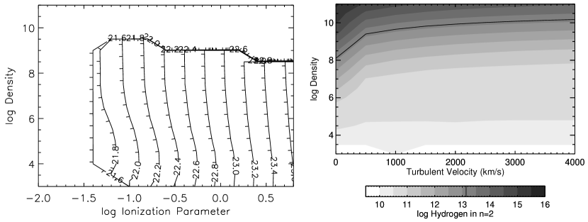
Figure 22: The results depend on the differential velocity properties of the gas. Left: The total hydrogen column density required to produce the observed He I column density for $v_{turb}=1000\rm\,km\,s^{-1}$. The hydrogen column densities are nearly the same as those shown in Fig. 8 ($v_{turb}=0$), except that the allowed parameter space extends to higher densities. Right: The column density of hydrogen in $n=2$ for $\log U=-1.0$ as a function of $v_{turb}$ and density for models where the hydrogen column density is chosen to produce the observed He I*. Ly$\alpha$ trapping is more important at high densities, resulting in an increase in hydrogen in $n=2$. The decrease in H I in $n=2$ as a function of $v_{turb}$ is a consequence of the suppression of Ly$\alpha$ trapping when turbulence is present. The solid line shows the upper limit on H I $n=2$ obtained from the lack of Balmer absorption.

Initially, we include $v_{turb}=1000\rm\,km\,s^{-1}$ in the model. We found that the execution time increased with $v_{turb}$, so we chose this value to start with. As discussed in §3.1, we ran models using a large column density, used the output to determine the column density required to produce the He I* column density measured from the data, then ran the models again. The grid sampled a slightly smaller range of ionization parameter than in §3.1, as Cloudy crashed for the highest ionization parameters where $\log U>\sim 0.8$. The results are shown in Fig. 22. Comparing this figure with Fig. 8, we see that the column densities are nearly the same, as well as the ionization constraint on the allowed parameter space. But higher densities are allowed, up to $\log n=9.5$ for $\log U\sim-1.0$. This happens because as $v_{turb}$ increases, Ly$\alpha$ is less trapped, so the column density of H Iin $n=2$ decreases, and so the upper limit on H I in $n=2$ is attained at higher densities.

We note that we see no evidence for destruction of He I* by Ly$\alpha$. If that were important, we would expect an increase in required hydrogen column at high densities, because we would have to go deeper into the gas to attain sufficient He I*. Exploratory Cloudy modeling showed that such an increase in total hydrogen column is only seen at $v_{turb}=0$ for very large densities, i.e., $\log n>~{}10$.

Fig. 22 also shows the column density of H I in $n=2$ for $\log U=-1$ as a function of turbulent velocity between 0 and 4000$\,\rm km\,s^{-1}$. Again, the total hydrogen column density has been adjusted to provide the observed He I*, and that is nearly constant, lying between 21.91 and 22.06. This graph shows that, for constant higher densities, after an initial decrease in H I $n=2$ column density as a function of $v_{turb}$, the dependence levels off so that the column density in H I $n=2$ at $v_{turb}=3000\rm\,km\,s^{-1}$ is nearly the same as that at $v_{turb}=4000\rm\,km\,s^{-1}$. Therefore, our upper limit on Balmer absorption lines seems to still rule out very high densities, even when a differential velocity field is present.

Figure 2: SpeX spectrum of FBQS J1151$+$3822 along with the comparison object spectra that have been normalized and scaled (see text for details).

Figure 6: Partial covering model of the IRTF ratio and the SDSS ratio extracted using the 28-spectrum Fe II model. The results for the excess-variance Fe II model and for the MDM ratio spectrum are similar. The top panel shows the ratios with the best-fitting model overlaid. The second and third panels show the fitted optical depth and covering fraction. The bottom panel shows the incremental column density as a function of velocity computed from the average optical depth in each velocity bin.

Figure 8: Total hydrogen column density obtained from Cloudy modeling. At each point, the hydrogen column was adjusted until the He I* average column was obtained. Insufficient He I* was produced for ionization parameters lower than $\sim-1.4$. High densities predict Balmer absorption in excess of the lower limit derived from the spectra.

Figure 10: Ratio of simulated spectrum to continuum for three combinations of density and ionization parameter from Fig. 21; these are listed on the y axes. The name of the absorption line is listed above the spectra, centered at the rest wavelength. Ionization parameter discrimination is straightforward: P V is much stronger at high ionization parameters, while low-ionization lines such as Mg II, C II, and S III are stronger at low ionization parameters. Blending makes density discrimination more difficult, but C III*$\lambda 1176$ is present at low ionization parameters and high densities.

Table 1: Inhomogeneous Absorber Model Fitting Results

Spectrum	Points Retained	Partial Covering Model	Power Law Model
		log He I* Column Density	log He I* Column Density
MDM – 28 spectra	63	$14.9^{+0.6}_{-0.2}$	$15.0^{+0.2}_{-0.1}$
MDM – excess variance	61	$14.8^{+0.9}_{-0.2}$	$14.8^{+0.2}_{-0.1}$
SDSS – 28 spectra	64	$15.0^{+0.8}_{-0.2}$	$15.1^{-0.2}_{-0.2}$
SDSS – excess variance	62	$14.9^{+0.8}_{-0.2}$	$15.0^{+0.2}_{-0.2}$

References

- Arav (1996) Arav, N. 1996, ApJ, 465, 617
- Arav et al. (1995) Arav, N., Korista, K. T., Barlow, T. A., & Begelman, M. C. 1995, Nature, 376, 576
- Arav & Li (1994) Arav, N., & Li, Z.-Y. 1994, ApJ, 427, 700
- Arav et al. (1994) Arav, N., Li, Z.-Y., & Begelman, M. C. 1994, ApJ, 432, 62
- Arav et al. (2005) Arav, N., Kaastra, J., Kriss, G. A., Korista, K. T., Gabel, J., & Proga, D. 2005, ApJ, 620, 665
- Bentz et al. (2006) Bentz, M. C., Peterson, B. M., Pogge, R. W., Vestergaard, M., & Onken, C. A. 2006, ApJ, 644, 133
- Bethe & Salpeter (1957) Bethe, H. A., & Salpeter, E. E. 1957, “Quantum Mechanics of One- and Two-Electron Atoms” (New York: Academic Press)
- Boroson & Green (1992) Boroson, T. A., & Green, R. F. 1992, ApJS, 80, 109
- Boksenberg et al. (1997) Boksenberg, A., Carswell, R. F., Allen, D. A., Fosbury, R. A. E., Penston, M. V., & Sargent, W. L. W. 1997, MNRAS, 178, 451
- Breit & Teller (1940) Breit, G., & Teller, E. 1940, ApJ, 91, 215
- Cardelli et al. (1989) Cardelli, J. A., Clayton, G. C., & Mathis, J. S. 1989, ApJ, 345, 245
- Casebeer et al. (2006) Casebeer, D. A., Leighly, K. M., & Baron, E. 2006, ApJ, 637, 157
- Castor et al. (1975) Castor, J. I., Abbott, D. C., & Klein, R. I. 1975, ApJ, 195, 175
- Cavaliere et al. (2002) Cavaliere, A., Lapi, A., & Menci, N. 2002, ApJ, 581, L1
- Clegg (1987) Clegg, R. E. S. 1987, MNRAS, 229, 31
- Clegg & Harrington (1989) Clegg, R. E. S., & Harrington, J. P. 1989, MNRAS, 239, 869
- Collin et al. (2006) Collin, S., Kawaguchi, T., Peterson, B. M., & Vestergaard, M. 2006, A&A, 456, 75
- Cottis et al. (1010) Cottis, C. E., Goad, M. R., Knigge, C., & Scaringi, S. 2010, MNRAS, accepted
- Crenshaw et al. (2003) Crenshaw, D. M., Kraemer, S. B., & George, I. M. 2003, ARA&A, 41, 117
- Cushing et al. (2004) Cushing, M. C., Vacca, W. D., & Rayner, J. T. 2004, PASP, 116, 362
- Dai et al. (2008) Dai, X., Shankar, F., & Sivakoff, G. R. 2008, ApJ, 672, 108
- De Kool et al. (2002) De Kool, M., Korista, K. T., & Arav, N. 2002, ApJ, 580, 54
- Drake (1971) Drake, G. W. F., 1971, Phys. Rev. A, 3, 908
- Drake & Dalgarno (1968) Drake, G. W. F., & Dalgarno, A. 1968, ApJ, 152, 121
- Drake et al. (1969) Drake, G. W. F., Victor, G. A., & Dalgarno, A. 1969, Physical Review, 180, 25
- Dunn et al. (2010) Dunn, J. P., Bautista, M., Arav, N., Moe, M., Korista, K., Constantini, E., Benn, C., Ellison, S., & Edmonds, D. 2010, ApJ, 709, 611
- Edwards et al. (2003) Edwards, S., Fischer, W., Kwan, J., Hillenbrand, L., & Dupree, A. K., 2003, ApJ, 599, 41
- Everett (2005) Everett, J. E. 2005, ApJ, 631, 689
- Ferland et al. (1998) Ferland, G. J., Korista, K. T., Verner, D. A., Ferguson, J. W., Kingdon, J. B. & Verner, E. M., 1998, PASP, 110, 761
- Gabriel & Jordon (1969) Gabriel, A. H., & Jordon, C. 1969, Nature, 221, 947
- Gallagher & Everett (2007) Gallagher, S. C., & Everett, J. E. 2007, ASPC, 373, 305
- Ganguly et al. (2007) Ganguly, R., Brotherton, M. S., Cales, S., Scoggins, B., Shang, Z., & Vestergaard, M. 2007, ApJ, 665, 990
- Gaskell (2008) Gaskell, C. M., 2008, RMxAA, 32, 1
- Gibson et al. (2009) Gibson, R. R., et al. 2009, ApJ, 692, 758
- Grevesse et al. (2007) Grevesse, N., Asplund, M., & Sauval, A. J. 2007, Space Sci. Rev., 130, 105
- Griem (1969) Griem, H. R. 1969, ApJ, 156, 103
- Hall et al. (2003) Hall, P. B., Hutsemékers, D., Anderson, S. F., Brinkmann, J., Fan, X., Schneider, D. P., & York, D. G. 2003, ApJ, 593, 189
- Hamann (1997) Hamann, F. 1997, ApJS, 109, 279
- Hamann (1998) Hamann, F. 1997, ApJ, 500, 798
- Hamann et al. (1997) Hamann, F., Barlow, T. A., Junkkarinen, V., & Burbidge, E. M. 1997, ApJ, 478, 80
- Hamann & Ferland (1999) Hamann, F., & Ferland, G. 1999, ARA&A, 37, 487
- Hamann et al. (2001) Hamann, F. W., Barlow, T. A.., Chaffee, F. C., Foltz, C. B., & Weymann, R. J., 2001, ApJ, 550, 142
- Hamann et al. (2002) Hamann, F., Korista, K. T., Ferland, G. J., Warner, C., & Baldwin, J. 2002, ApJ, 564, 592
- Hamann et al. (2010) Hamann, F., Kanekar, N., J. X. Prochaska, Murphy, M. T., Ellison, S., Malec, A. L., Milutinovic, N., & Ubachs, W., 2010, MNRAS in press
- Korista et al. (1997) Korista, K. T., Baldwin, J., Ferland, G., & Verner, D. 1997, ApJS, 108, 401
- Korista et al. (1993) Korista, K. T., Voit, G. M., Morris, S. L., & Weymann, R. J. 1993, ApJS, 88, 357
- Kraemer et al. (2001) Kraemer, S. B., Crenshaw, D. M., Hutchings, J. B., George, I. M., Danks, A. C., Gull, T. R., Kaiser, M. E., Nelson, C. H., Weistrop, D., & Vieira, G. L. 2001, ApJ, 551, 671
- Kraemer et al. (2006) Kraemer, S. B., et al. 2006, ApJS, 167, 161
- Kriss et al. (1992) Kriss, G. A., et al. 1992, ApJ, 392, 485
- Krolik & Kriss (2001) Krolik, J. H., & Kriss, G. A. 2001, ApJ, 561, 684
- Landt et al. (2008) Landt, H., Bentz, M. C., Ward, M. J., Elvis, M., Peterson, B. M., Korista, K. T., & Karovska, M. 2008, ApJS, 174, 282
- Laor & Brandt (2002) Laor, A., & Brandt, W. N., 2002, ApJ, 569, 641
- Laor et al. (1997) Laor, A., Jannuzi, B. T., Green, R. F., & Boroson, T. A., 1997, ApJ, 489, 656
- Leighly et al. (2009) Leighly, K. M., Hamann, F., Casebeer, D. A., & Grupe, D. 2009, ApJ, 701, 176
- Leighly et al. (2007) Leighly, K. M., Halpern, J. P., Jenkins, E. B., & Casebeer, D. 2007, ApJS, 173, 1
- Mathis (1957) Mathis, J. S. 1957, ApJ, 125, 318
- North et al. (2006) North, M., Knigge, C., & Goad, M. 2006, MNRAS, 365, 1057
- Ogle (1998) Ogle, P. M., Ph. D. Thesis, California Institute of Technology 1998
- Pei (1992) Pei, Y. C., 1992, ApJ, 395, 130
- Phillips (1978) Phillips, M. M., 1978, ApJ, 226, 736
- Proga & Kallman (2004) Proga, D., & Kallman, T. R. 2004, ApJ, 616, 688
- Proga et al. (2000) Proga, D., Stone, J. M., & Kallman, T. R. 2000, ApJ, 543, 686
- Rayner et al. (2003) Rayner, J. T., Toomey, D. W., Onaka, P. M., Denault, A. J., Stahlberber, W. E., Vacca, W. D., Cushing, M. C., & Wang, S. 2003, PASP, 115, 362
- Richards et al. (2006) Richards, G. T., et al. 2006, ApJS, 166, 470
- Sabra & Hamann (2005) Sabra, B. M., & Hamann, F., 2005, arXiv:astro-ph/0509421
- Saraph & Storey (1999) Saraph, H. E., & Storey, P. J. 1999, A&AS, 143, 369
- Savage & Sembach (1991) Savage, B. D., & Sembach, K. R. 1991, ApJ, 379, 245
- Scannapieco & Oh (2004) Scannapieco, E., & Oh, S. P. 2004, ApJ, 608, 62
- Schlegel et al. (1998) Schlegel, D. J., Finkbeiner, D. P., & Davis, M. 1998, ApJ, 500, 525
- Schneider et al. (2010) Schneider, D. et al. 2010, AJ, 139, 2360
- Scoville & Norman (1995) Scoville, N., & Norman, C. 1995, ApJ, 451, 510
- Sulentic et al. (2006) Sulentic, J. W., Dultzin-Hacyan, D, Marziani, P., Bongardo, C., Braito, V., Calvani, M., & Zamanov, R. 2006, RMxAA, 42, 23
- Turnshek et al. (1997) Turnshek, D. A., Monier, E. M., Sirola, C. J., & Espey, B. R. 1997, ApJ, 476, 40
- Vacca et al. (2003) Vacca, W. D., Cushing, M. C., & Rayner, J. T. 2003, PASP, 115, 389
- Verner et al. (1994) Verner, D. A., Barthel, P. D., & Tytler, D. 1994, A&AS, 108, 287
- Verner et al. (1999) Verner, E. M., Verner, D. A., Korista, K. T., Ferguson, J. W., Hamann, F., & Ferland, G. J. 1999 ApJS, 120, 101
- Weymann et al. (1991) Weymann, R. J., Morris, S. L., Foltz, C. B., & Hewett, P. C. 1991, ApJ, 373, 23
- White et al. (2000) White, R. L., et al. 2000, ApJS, 126, 133