Irrelevance of information outflow in opinion dynamics models

Abstract

The Sznajd model for opinion dynamics has attracted a large interest as a simple realization of the psychological principle of social validation. As its most salient feature, it has been claimed that the Sznajd model is qualitatively different from other ordering processes, because it is the only one featuring outflow of information as opposed to inflow. We show that this claim is unfounded by presenting a generalized zero-temperature Glauber-type of dynamics which yields results indistinguishable from those of the Sznajd model. In one-dimension we also derive an exact expression for the exit probability of the Sznajd model, that turns out to coincide with the result of an analytical approach based on the Kirkwood approximation. This observation raises interesting questions about the applicability and limitations of this approach.

In the last decades statistical physics has crossed many boundaries between different fields, becoming, with its methods and concepts, a powerful tool for the investigation of a broad range of disciplines. This process has been mutually beneficial, since the consideration of problems far away from a purely physical motivation has greatly broadened the kind of theoretical questions and conceptual challenges statistical physics is called to tackle. One of the settings in which this cross-fertilization has been particularly fruitful is opinion dynamics Castellano et al. (2009), where the goal is to understand how global consensus/understanding/agreement emerges out of disorder, based on local interactions. In this field many simple models akin to those of statistical physics have been introduced, both by social scientists and physicists Clifford and Sudbury (1973); Axelrod (1997); Galam et al. (1982); Deffuant et al. (2000); Krapivsky and Redner (2003), leading to intense activity and remarkable results. In this context, the model introduced by Sznajd-Weron and Sznajd Sznajd-Weron and Sznajd (2000), commonly denoted as Sznajd model (SM), has enjoyed an exceptional success as the first one encoding the principle of “social validation”, stating that the convincing power of an individual is greatly enhanced if another individual supports the same view.

The dynamics of the SM in one dimension is defined as follows Sznajd-Weron (2005); Stauffer et al. (2000): Each site in a one dimensional lattice is endowed with a binary variable (spin) $\sigma_{i}=\pm 1$. At each time step a pair of neighboring sites is selected at random, $i$ and $i+1$. If these individuals have the same opinion, $\sigma_{i}=\sigma_{i+1}\equiv\sigma$, the opinion of all the neighbors of $i$ and $i+1$ changes to the common value $\sigma$; otherwise, nothing happens . The process is iterated until, on a finite system, a final consensus (all spins equal) is reached. Generalizations to higher dimensions have been introduced and are described below. Typical quantities of interest are the consensus (fixation) time $T(x,N)$, defined as the time needed to reach the state with all spins equal for a system of size $N$, starting from a configuration with a fraction $x$ of positive spins, and the exit probability $E(x)$, defined as the probability that the final state will be all $\sigma_{i}=+1$.

The Sznajd model is similar to other simple models for dynamics of Ising spins in the absence of bulk noise, such as the voter model and the zero temperature Glauber dynamics. However, much emphasis has been put Krupa and Sznajd-Weron (2005); Sznajd-Weron and Krupa (2006); Sousa and Sánchez (2006) on the claim that SM is fundamentally different because it is the only model where “information flows out” (i.e. spins propagate their state to their neighbors) as opposed to other models where a central spin adapts itself to the state of the surrounding ones (”information inflow”). This claim is mainly supported by the shape of $E(x)$ in one dimension, which is linear for the Glauber zero temperature dynamics (as well as for the voter model), while it is nontrivial for SM Lambiotte and Redner (2008); Slanina et al. (2008). Also the consensus time $T(x,N)$ has a dependence on $x$ for SM that is not found in other types of dynamics.

In this Letter we show this claim to be unfounded, by presenting two clearly “outflow” and “inflow” dynamics, given by simple extensions of the SM and the Glauber models, respectively, in which the number of sites involved in a single spin update is a model parameter. The analysis of these models allows us to check that the postulated difference between “inflow” and “outflow” dynamics in fact does not exist. In particular, we show that in one dimension the exit probabilities and consensus times of both models are the same. The consideration of the two dimensional and mean-field cases adds additional strength to our result. Additionally, we provide an exact expression for the exit probability of SM in one dimension, revealing that previous results based on a Kirkwood approximation are also exact, due to some surprising cancellation of errors that remains to be understood.

The models we consider are defined in one dimension as follows:

Sznajd Model of range $R$, $SM(R)$: At each time step, a pair of nearest neighbor sites, $i,i+1$, is chosen at random. If they share the same state, $\sigma_{i}=\sigma_{i+1}\equiv\sigma$, then the $2R$ neighbors, to left and right, respectively, change their value to $\sigma$, i.e. $\sigma_{j}\to\sigma$, for $j\in[i-R,i-1]\cup[i+2,i+1+R]$. Otherwise, nothing happens. In this “outflow” dynamics, the opinion of two adjacent equal spins thus extends to all their $2R$ neighbors, the case $R=1$ corresponding to the standard SM.

Zero temperature Glauber dynamics of range $R$, $G(R)$: The elementary step consists in randomly selecting a site $i$ and evaluating the local field given by the sum of the $2R$ spins in the interval $[i-R,i-1]\cup[i+1,i+1+R]$. If the local field is positive or negative, the variable $\sigma_{i}$ aligns with it. Otherwise the spin is randomly set to $\pm 1$ with probability $1/2$. For any $R$ the dynamics is obviously of “inflow” type, as the central spin is affected by the state of surrounding spins. The case $G(1)$ coincides with the usual zero-temperature Glauber dynamics.

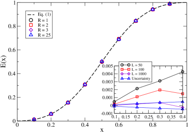
Figure 1: Main: Exit probability for the $SM(R)$ on a one dimensional lattice of size $L=1000$. The full line corresponds to the analytical prediction, Eq. (1). The number of realizations of the dynamics is $M=10^{5}$. Inset: Difference between the numerical results for $SM(1)$ and the theoretical as $L$ changes. The uncertainty due to sampling error for $L=1000$ is given by $\pm\sqrt{(}E(x)[1-E(x)]/M)$, where the number of realizations of the stochastic process is $M=10^{6}$.

Let us consider uncorrelated initial conditions in which each vertex has a probability $x$ to be in the $+1$ state, and correspondingly a probability $1-x$ to be in state $-1$. As in other ordering processes of this kind, the evolution in both $SM(R)$ and $G(R)$ models proceeds in two separate stages. Initially, homogeneous domains of spins up or down quickly form at small scale. This stage lasts for a time of the order of a few Monte Carlo steps per spin. Later on, domain boundaries diffuse around and annihilate upon encounter, leading to larger and larger domains and eventually to consensus. The duration of this second stage grows with the system size as $L^{2}$. While in the first stage the dynamics depends on the model’s microscopic details and the magnetization is not conserved, the second regime is very similar for voter, generalized SM or generalized Glauber models, with marginal variations due only to the details of the annihilation process. In this stage, the diffusion-annihilation boundary dynamics leads to the conservation of the average magnetization.

We first study the behavior of the $SM(R)$ model, plotting in Fig. 1 the exit probability for this model, computed numerically for different values of $R$. Remarkably, $E(x)$ turns out to be completely independent of the range of the interaction $R$. By taking advantage of this independence of $R$, we can derive the exact form of the exit probability, which is very easy to compute for $R\geq(L-2)/2$. In such a case, the diffusive regime is absent and the system becomes fully ordered after the first successful microscopic update. The dynamics proceeds by choosing at random $2$ consecutive sites, that will be both in state $+1$ with probability $x^{2}$, in state $-1$ with probability $(1-x)^{2}$, and in a mixed state with probability $1-x^{2}-(1-x)^{2}$. The exit probability is given by the probability that a pair of sites in state $+1$ is chosen before any pair of sites in state $-1$. So, we can write

$$E(x)=x^{2}\sum_{n=0}^{\infty}[1-x^{2}-(1-x)^{2}]^{n}=\frac{x^{2}}{x^{2}+(1-x)^{2}}.$$ (1)

Another way to derive Eq. (1), valid for smaller values of $R$, is as follows: In the initial stage each successful update will give rise to a domain of $2+2R$ equal sites, so that in a time of order unity the system will be roughly subdivided into $L/(2+2R)$ domains of size of order $2+2R$. At the end of this stage , the density of $+1$ spins will be $x^{\prime}=1\times x^{2}/[x^{2}+(1-x)^{2}]+0\times(1-x)^{2}/[x^{2}+(1-x)^{2}]$. In the ensuing second stage the conservation of magnetization implies that the exit probability is $E(x^{\prime})=x^{\prime}$, independent of domain size, yielding again Eq. (1).

Fig. 1 shows that Eq. (1) provides a very accurate description of the exit probability of the generalized SM. The inset of the figure proves moreover that the small deviations of the numerical results for $E(x)$ around the theoretical value can be fully ascribed to fluctuations around the expected value due to the finite number of realizations of the process. This confirms that Eq. (1) is the exact solution of the exit probability for the SM.

It is crucial to remark that Eq. (1) coincides with the expression for the exit probability of SM calculated by solving analytically the hierarchy of equations for multi-spin correlation functions within a Kirkwood approximation decoupling scheme Lambiotte and Redner (2008); Slanina et al. (2008). In this case then, the Kirkwood approximation turns out to provide an exact solution for the SM model. This is indeed a striking result, since numerical tests show that the assumptions made in the Kirkwood approximation are largely violated during the dynamics.

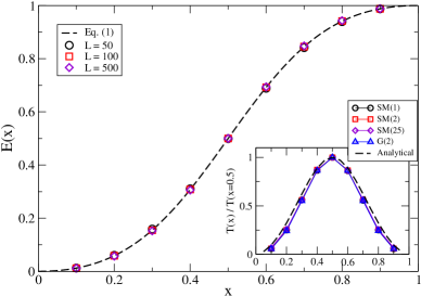
Figure 2: Exit probability for the $G(2)$ dynamics in one dimensional lattices of increasing size. The full line corresponds to the analytical prediction for the SM, Eq. (1). The number of realizations of the dynamics is $10^{6}$. Inset: Numerical values of the consensus time $T(x)$ rescaled by its maximum value $T(x=0.5)$, for $G(2)$ and $SM(R)$, compared with the analytical prediction (see text). Lattice size $L=500$.

Turning now to the generalized Glauber dynamics $G(R)$, numerical simulations for $R=2$ (Fig. 2) show that also in this case $E(x)$ is in excellent agreement with Eq. (1). Hence the exit probability of $SM(R)$ and of the $G(2)$ model are indistinguishable. The closeness of the two models is further confirmed by the inset of Fig. 2, where the consensus time $T(x)$ (divided by $T(x=0.5)$ to factor out trivial temporal rescalings) is reported: The time needed to reach the final consensus is the same for both $SM(R)$ and $G(R=2)$ models. Fig. 2 provides further evidence of the independence of the generalized SM with $R$ and allows to conclude that direction of “information flow” is irrelevant: The behavior of Sznajd model with “outflow” dynamics coincides with the behavior of $G(R=2)$ model, based on “inflow”.

The dynamical division in two stages, illustrated above to derive the exit probability, is useful also to obtain an analytical estimate of the time $T(x)$ to reach consensus for the SM. As described above, in a time of order unity the density of $+1$ spins reaches its asymptotic value $x^{\prime}=x^{2}/[x^{2}+(1-x)^{2}]$, where $x$ is the magnetization in the initial state. The ensuing evolution is essentially the same followed by the voter model, for which the consensus time is known and whose dependence on the initial density of up spins $x^{\prime}$ is $T\propto-[x^{\prime}\ln x^{\prime}+(1-x^{\prime})\ln(1-x^{\prime})]$. Expressing $x^{\prime}$ in terms of the initial value $x$ one obtains an analytical formula for the consensus time of the SM. The comparison with numerics (Fig. 2, inset) is rather good, the discrepancy observed being probably ascribable to the slightly different behavior of the models when two boundaries are one site far apart. While in the voter dynamics they have equal probability to collide or to go to distance 2, they deterministically collide in SM.

The strong relationship between the $G(2)$ and SM is not limited to one-dimensional systems. Let us consider a random neighbor topology, i.e. a fully connected system where the interaction occurs with neighbors chosen randomly at each time step. Slanina and Lavicka Slanina et al. (2008) have analyzed the standard Sznajd dynamics in this case, characterized by the transition rates

$$\textrm{Prob}[x\to x+1/N] = x^{2}(1-x),$$ (2a)

$$\textrm{Prob}[x\to x-1/N] = x(1-x)^{2},$$ (2b)

where $N$ is the system size. For the generalized Glauber $G(2)$ dynamics the rates can be also easily worked out

$$\textrm{Prob}[x\to x+1/N] = x^{2}(1-x)(3-2x),$$ (3a)

$$\textrm{Prob}[x\to x-1/N] = x(1-x)^{2}(1+2x).$$ (3b)

The only variation is given by correcting factors which are smooth and positive, thus implying that no basic feature of the dynamics will change. In particular, following the inverse Fokker-Planck formalism Gardiner (1985), it is possible to show that the exit probability takes in both cases the form of a Heaviside step function, $E(x)=\Theta(x-0.5)$ for $N\to\infty$, as expected due to the presence of an imbalance between the rates in Eqs. (2) and (3).

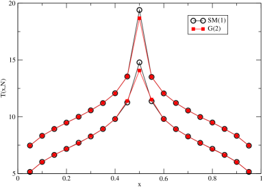
Figure 3: Consensus time $T(x,N)$ as a function of the initial fraction $x$ of $+1$ spins, for $SM(1)$ and $G(2)$ models on a random neighbor topology. Upper curves are for size $N=10^{4}$. Lower curves are for size $N=10^{3}$.

Concerning the consensus time, we report the results of computer simulations in Fig. 3, which prove the equivalence between the SM and the $G(2)$ models at the mean-field level.

In finite dimensions larger than one, many possible ways to define SM have been introduced Stauffer et al. (2000); Krupa and Sznajd-Weron (2005); Kondrat and Sznajd-Weron (2008). Similarly, there are various possibilities to define the Glauber dynamics for generic $R$. We select the following ones. For the $G(R)$ model, the local field for a site $(i,j)$ is given by the sum of all spins up to the $R$-nearest neighbors. In particular for $R=2$ in $d=2$ the local field is given by the sum of the eight spins surrounding $(i,j)$ and forming together a square of side $3$. For the SM, on the other hand, we consider two variants. In SM-I dynamics a bond is randomly chosen, either along the vertical or horizontal direction, and if the sites at the extremes of the bond are equal, all the 6 nearest neighbors of both sites are updated accordingly. In SM-II, we select a plaquette of four sites and if they are in same state, the 8 nearest neighbors are made equal.

The probability $E(x)$ to end up with all $+1$ spins is for all variants of SM given (in the large size limit) by a step function $E(x)=\Theta(x-0.5)$ Stauffer et al. (2000). As can be expected based on the fact that the dynamics is driven by curvature Bray (1994), the same occurs for the $G(2)$ model, provided no freezing in a striped configuration occurs Spirin et al. (2001). This phenomenon, which affects asymptotically $G(1)$ dynamics in $d=2$ with a finite probability Spirin et al. (2001) (and clearly affects $G(2)$ dynamics as well), is present also in the evolution of the SM. In this case, straight stripes along one direction in a two-dimensional lattice are not fully stable, given the intrinsic destabilizing mechanism present in Sznajd dynamics at microscopic scales. Nevertheless stripes do often form during the evolution and they persist for very long times.

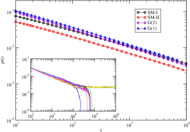
Figure 4: Density $\rho(t)$ in $d=2$ for SM-I, SM-II, $G(1)$, and $G(2)$ dynamics. System size $L=10000$. Inset: $\rho(t)$ for several runs on a SM-I system of size $L=1000$, illustrating the stripe phenomenon.

The presence of stable or long lived metastable striped states makes a comparison between the consensus time $T(x,N)$ in SM and Glauber $G(R)$ models impossible. A quantity allowing a better analysis of the ordering behavior of two-dimensional systems is the fraction $\rho(t)$ of nearest neighbor pairs that are in opposite states. Figure 4 shows that for Sznajd and generalized Glauber dynamics (with both $R=1$ or $R=2$) the evolution is the same, apart from irrelevant transients and global temporal scales: The density $\rho$ decreases as $t^{-1/2}$, the signature of curvature-driven coarsening dynamics Bray (1994). On the other hand, the plateaus exhibited in some realizations of Sznajd dynamics for long times (Fig. 4, inset) indicate the effective presence of long-lived metastable states. The perfect analogy between Sznajd and Glauber dynamics goes beyond the decay of $\rho(t)$. The scaling functions for the two-point correlation function $C(r,t)$ (not shown) are virtually the same.

In summary, we have shown that the behavior of Sznajd model for opinion dynamics has no feature that distinguishes it from a generalized zero temperature Glauber dynamics for Ising spins. While in dimension $d>1$ this could be expected on the basis of general considerations on coarsening systems, in $d=1$ this result is highly nontrivial. In one-dimensional systems, the standard Sznajd dynamics actually differs from the usual zero-temperature Glauber dynamics, as it has been extensively reported in the literature. However, when the range of the interactions is extended to $R=2$, the generalized Glauber dynamics is indistinguishable from Sznajd. The conclusion is that “outflow” dynamics is not qualitatively different from “inflow” dynamics. A possible objection to this conclusion is that inflow and outflow dynamics are actually different because $SM(R)$ does not depend on $R$, while $G(R)$ dynamics does. This argument is rebutted by considering another extension of SM, in which the number of equal spins needed to convince neighbors is a parameter $q$. Numerical and analytical arguments, to be reported elsewhere Pastor-Satorras and Castellano (2010), show that $q$ strongly affects the dynamics and that such a generalized “outflow” dynamics gives results very close to those of the $G(R)$ “inflow” model with $R=q$. While studying the equivalence of $SM(R)$ and $G(2)$ we have derived an exact formula for the exit probability of SM, that turns out to coincide with the one obtained by using a Kirkwood approximation. Notice that, on the contrary, Kirkwood approximation fails for the $G(2)$ dynamics Pastor-Satorras and Castellano (2010). These findings call for additional research to understand when the Kirkwood approximation works, when it fails, and how it can be systematically improved.