Cyclotron resonance and Faraday rotation in graphite

Abstract

The optical conductivity of graphite in quantizing magnetic fields is analytically evaluated for frequencies in the range of 10–300 meV, where the electron relaxation processes can be neglected and the low-energy excitations at the ”Dirac lines” are more essential. The conductivity peaks are explained in terms of the electron transitions in graphite. Conductivity calculated per one graphite layer tends on average to the universal conductivity of graphene. The (semi)metal-insulator transformation is possible under doping in high magnetic fields.

Graphite is usually considered as a layered semimetal composed of the graphene monolayers. Within this assumption, the graphite electron spectrum was evaluated many years ago within the Slonczewski–Weiss–McClure (SWM) theory SW . The so called ”Dirac cone” turns into four bands with the twofold degenerate zero mode where electrons and holes are located Sem . The zero-mode dispersion is very small, of the order of 20 meV, in the main-axis direction because the interlayer interaction is weak. Unusual properties of graphite have attracted much attention for more than 50 years. The most accurate method to study the band structure of graphite is a study of the Landau levels (LLs) through experiments such as magneto-optics TDD ; DDS ; LTP ; OFM ; OFS ; OP ; CLW and magnetotransport KTS ; LK ; JZS ; SOP ; RM . However, the interpretation of the experimental results involves a significant degree of uncertainty since, as noticed by Doezema et al DDS and Chuang at al CBN ”it is not clear where the resonances are to be marked.”

The SWM theory requires the use of many tight-binding parameters and provides the simple description of observed phenomena either in the semiclassical limit of week magnetic fields or for high frequencies when the largest tight-binding parameter $\gamma_{1}=0.4$ eV plays the leading role Fal . At the relatively strong magnetic fields $B\sim$ 1–30 T and frequencies $\omega\sim$ 10–350 meV, the smaller tight-binding parameters $\gamma_{2},\gamma_{5},$ and $\Delta$ of the order of 20 meV are essential. In this case, any physical property for graphite in magnetic field is represented by an integral over the momentum projection $k_{z}$. The SWM model can be simplified assuming that only the integration limits produce the main contributions OFS ; CBN ; LA . Such approximation is similar to the theory of magneto-optical effects in topological insulators TM and graphene MHA . However, in the 3d systems, the other features such as the band extrema or the integration limits at the Fermi level can contribute as well. Therefore, the analytical expression for the dynamic conductivity in the presence of magnetic fields is needed for an interpretation of magneto-optics experiments. The theoretical study of magneto-optical properties in multilayer graphene is realized in Ref. KA .

In this paper, we evaluate a formula for the optical conductivity of graphite in the presence of quantizing magnetic fields and results are compared with experiments. We remind the notation for the LLs in graphite using the Hamiltonian in the form of Refs. PP ; GAW . The expression for both the longitudinal and Hall dynamical conductivities is given. The (semi)metal–insulator transition is discussed in conclusions.

Neglecting the trigonal warping $\gamma_{3}$, the effective Hamiltonian near the $KH-$line of the Brillouin zone can be written in the form

$$H(\mathbf{k})=\left(\begin{array}[]{cccc}\tilde{\gamma}_{5}&vk_{+}&\tilde{\gamma}_{1}&0\\ vk_{-}&\tilde{\gamma}_{2}&0&0\\ \tilde{\gamma}_{1}&0&\tilde{\gamma}_{5}&vk_{-}\\ 0&0&vk_{+}&\tilde{\gamma}_{2}\end{array}\right)$$ (1)

where $k_{\pm}=\mp ik_{x}-k_{y}$, $v=1.02\times 10^{8}$ cm/s is the intra-layer velocity, and $\tilde{\gamma}_{j}$ are the functions of $k_{z}$:

$$\tilde{\gamma_{1}}=2\gamma_{1}\cos{(k_{z}c_{0})}\,,\tilde{\gamma}_{2}=2\gamma_{2}\cos{(2k_{z}c_{0})}\,,$$

$$\tilde{\gamma}_{5}=2\gamma_{5}\cos{(2k_{z}c_{0})}+\Delta$$

with the distance $c_{0}=3.35$ Å  between layers in graphite.

At the magnetic field $B$, the momentum projections $k_{x,y}$ become the operators with the commutation rule $\{k_{+},k_{-}\}=-2e\hbar B/c$, and we can use the relations

$$k_{+}=\sqrt{2|e|\hbar B/c}\,a,\quad k_{-}=\sqrt{2|e|\hbar B/c}\,a^{+}\,,$$

involving the creation and annihilation operators. We seek the eigenfunction of the Hamiltonian in the form

$$\psi_{sn}^{\alpha}(x)=\left\{\begin{array}[]{c}C^{1}_{sn}\varphi_{n-1}(x)\\ C^{2}_{sn}\varphi_{n}(x)\\ C^{3}_{sn}\varphi_{n-1}(x)\\ C^{4}_{sn}\varphi_{n-2}(x)\end{array}\right.$$ (2)

where the Landau number $n\geq 2$ and $\varphi_{n}(x)$ are orthonormal Hermitian functions with $n\geq 0$. Then, every row in the Hamiltonian (1) becomes proportional to the Hermitian function with the definite $n$, and we obtain a system of the linear equations for the eigenvector ${\bf C}_{sn}$

$$\left(\begin{array}[]{cccc}\tilde{\gamma}_{5}-\varepsilon&\omega_{c}\sqrt{n}&\tilde{\gamma}_{1}&0\\ \omega_{c}\sqrt{n}&\tilde{\gamma}_{2}-\varepsilon&0&0\\ \tilde{\gamma}_{1}&0&\tilde{\gamma}_{5}-\varepsilon&\omega_{c}\sqrt{n-1}\\ 0&0&\omega_{c}\sqrt{n-1}&\tilde{\gamma}_{2}-\varepsilon\end{array}\right)\times\left(\begin{array}[]{c}C^{1}_{sn}\\ C^{2}_{sn}\\ C^{3}_{sn}\\ C^{4}_{sn}\end{array}\right)=0\,$$ (3)

where $\omega_{c}=v\sqrt{2|e|\hbar B/c}$.

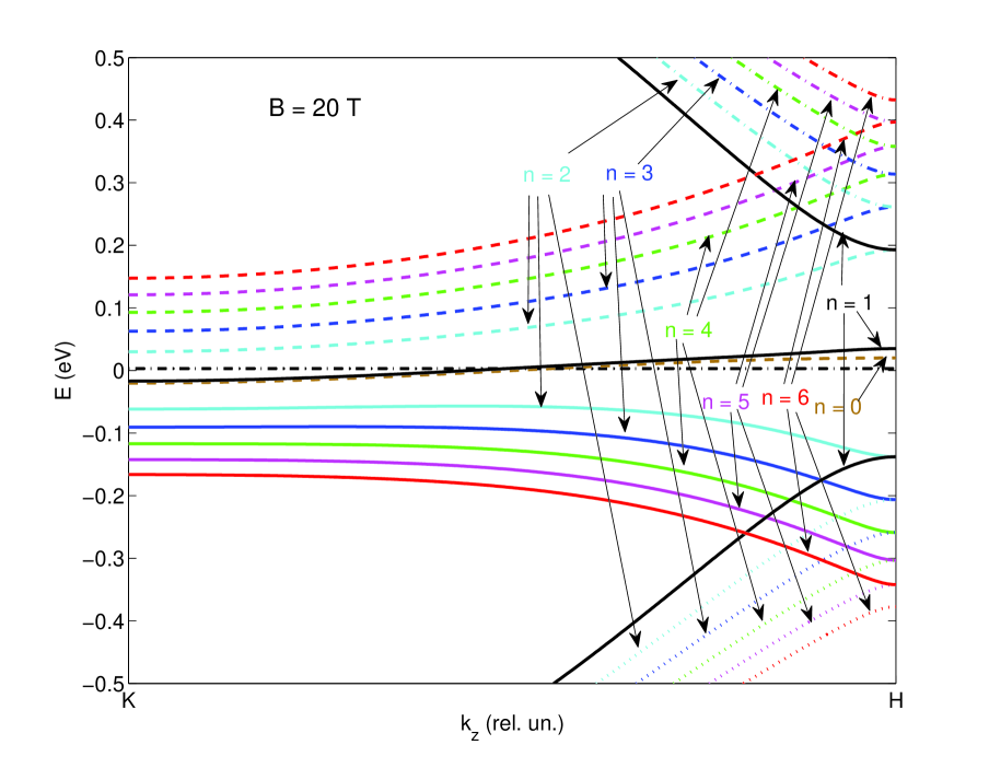
Figure 1: (Color online) LLs $\varepsilon_{sn}$ for $n$ = 0 to 6 in four bands $s$ as functions of momentum $k_{z}$ along the $KH-$line in the Brillouin zone ($K=0,\,H=\pi/2c_{0}$) at the magnetic field $B$ = 20 T using the SWM model with the TB parameters taken from Refs. PP ; GAW and neglecting trigonal warping; the Fermi energy $\varepsilon_{F}=0$ eV shown in dash-dotted line. Electron transitions are possible between the levels $\varepsilon_{sn}<0$ and $\varepsilon_{s^{\prime}n^{\prime}}>0$ with the selection rule $\Delta n=\pm 1$ .

At each Landau number $n$, the eigenvalues $\varepsilon_{sn}$ of the Hamiltonian are marked by the index of the band $s=1,2,3,4$ numerating the levels from the bottom. We will use the notation $|sn\rangle$ for levels. LLs with $n\geq 2$ are in every four bands, shown in Fig. 1 as functions of $k_{z}$ along the $KH-$line of the Brillouin zone. The eigenvalues are determined by the equation

$$[(\tilde{\gamma}_{5}-\varepsilon)(\tilde{\gamma}_{2}-\varepsilon)-\omega_{c}^{2}(n-1)]$$

$$\times[(\tilde{\gamma}_{5}-\varepsilon)(\tilde{\gamma}_{2}-\varepsilon)-\omega_{c}^{2}n]-\tilde{\gamma}_{1}^{2}(\tilde{\gamma}_{2}-\varepsilon)^{2}=0\,.$$

In addition, there are four levels. One of them, $\varepsilon_{0}=\tilde{\gamma}_{2}$, with $n=0$ and the eigenvector ${\bf C}_{0}=(0,1,0,0).$ This level intersects the Fermi level and belongs to the electron (hole) band near the $K$ $(H)$ point. Other three levels, $s=1,2,3,$ are indicated by $n=1$ with $C^{4}_{s1}=0$. One level, $|21\rangle$, is very close to the level with $n=0$. This pattern is consistent with Ref. OFM . The level structure at the $K^{\prime}H^{\prime}-$line is similar, therefore each level is fourfold degenerate, twice in spin and twice in pseudo-spin of the $KH$ and $K^{\prime}H^{\prime}$ valleys.

In the region, where $\tilde{\gamma}_{1}\gg\tilde{\gamma}_{2},\tilde{\gamma}_{5}$, the two closest bands are written as

$$\varepsilon_{2,3}(n)=\tilde{\gamma_{2}}\pm\omega_{c}^{2}\sqrt{n(n-1)}/\tilde{\gamma}_{1}\,.$$

The Fermi energy at zero temperature, $T$=0, is determined by equality of electron and hole concentrations given by the sum of integrals

$$n_{h,e}=\frac{\hbar\omega_{c}^{2}}{\pi^{2}v^{2}c_{0}}\sum_{sn}\int dz$$ (4)

over the region in the Brillouin half-zone $z=c_{0}k_{z}$ where electrons and holes are located. As known, the Fermi energy oscillates in the quantum Hall regime. We will consider the relatively strong magnetic fields where the oscillations do not exceed of 2 meV according to the electro-neutrality condition (4).

At finite temperatures the conductivity is expressed in terms of the correlation function AGD (for details see Ref. FV )

$$\mathcal{P}\left(\omega\right)=T\sum\limits_{\omega_{m}}\int dxdx^{\prime}Tr\left\{v^{i}\mathcal{G}\left(\omega_{+},x,x^{\prime}\right)v^{j}\mathcal{G}\left(\omega_{-},x^{\prime},x\right)\right\}\,,$$ (5)

where $\mathcal{G}\left(\omega_{+},x,x^{\prime}\right)$ is the temperature Green’s function, $\omega_{\pm}=\omega\pm\omega_{m}$ , $Tr$ is taken over the $|sn\rangle-$eigenstates, and the $x,x^{\prime}-$integration is over the coordinate involved explicitly in the Hamiltonian while the Landau gauge is used. Then, the Fourier transform of the eigenstates with respect the $y-$coordinate is assumed. Using the eigenfunctions (2), we write the Green’s function of the Hamiltonian (1)

$$\mathcal{G}^{\alpha\beta}(\omega,x,x^{\prime})=\sum_{sn}\frac{\psi^{\alpha}_{sn}(x)\psi^{*\beta}_{sn}(x^{\prime})}{i\omega-\varepsilon_{sn}}\,.$$

The intralayer-velocity matrix $v^{i}$ is given by the derivative of the Hamiltonian (1)

$$\mathbf{v}=\frac{\partial H(\mathbf{k})}{\partial\mathbf{k}}\,.$$ (6)

The straightforward calculation of the dynamical conductivity gives

$$\left.\begin{array}[]{c}\sigma_{xx}(\omega)\\ i\sigma_{xy}(\omega)\end{array}\right\}=i{\displaystyle\sigma_{0}\frac{4\omega_{c}^{2}}{\pi^{2}}}{\displaystyle\sum_{n,s,s^{\prime}}\int\limits_{0}\limits^{\pi/2}\frac{dz}{\Delta_{ss^{\prime}n}}[f(\varepsilon_{s^{\prime}n+1})-f(\varepsilon_{s,n})}]$$ (8)

$$\times{\displaystyle\left[(\omega+i\Gamma+\Delta_{ss^{\prime}n})^{-1}\pm(\omega+i\Gamma-\Delta_{ss^{\prime}n})^{-1}\right]}$$ (9)

$$\times\left|C^{2}_{sn}C^{1*}_{s^{\prime}n+1}+C^{3}_{sn}C^{4*}_{s^{\prime}n+1}\right|^{2}\,,$$

where $\Delta_{ss^{\prime}n}=\varepsilon_{sn}-\varepsilon_{s^{\prime},n+1}$ is the level spacing, $\omega_{c}=v\sqrt{2|e|\hbar B/c}$ is the cyclotron frequency, and $f(\varepsilon)=[\exp(\frac{\varepsilon-\mu}{T})+1]^{-1}$ is the Fermi-Dirac function. The integration over the Brillouin half-zone, $0<z<\pi/2$, and the summation over the Landau number $n$ as well as the bands $s,s^{\prime}$ should be done in Eq. (9).

The selection rule $\Delta n=\pm 1$ appears as a result of integration over $x$ and $x^{\prime}$ in Eq. (5). If the trigonal warping is taken into account, the selection rule is changed No ; ST . Let us notice that the choice of the selection rule can be done examining the intensities of the cyclotron resonance lines. Our choice corresponds with observations in Refs. OFS ; CBN .

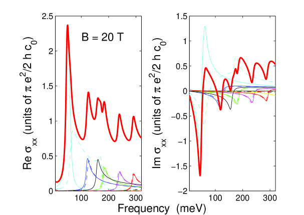
Figure 2: (Color online) Real and imaginary parts of the longitudinal dynamical conductivity at $B=$20 T (thick line); the partial contributions of various electron transition are shown in the thin lines. Temperature T=0.1 meV is less than the level broadening $\Gamma=5$ meV.

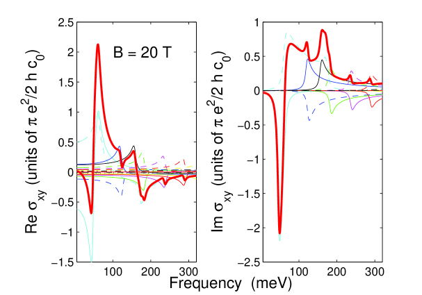
Figure 3: (Color online) Real and imaginary parts of the dynamical Hall conductivity at $B=$20 T (thick line) with the partial contributions of various electron transition shown in the thin lines.

The results for the longitudinal conductivity $\sigma_{xx}(\omega)$ are shown in Figs. 2 and 4 for two values of the magnetic field in order to compare the effect of the field. The dynamical Hall conductivity $\sigma_{xy}(\omega)$ shown in Figs. 3 and 5 describes the Faraday rotation CLW . The formula (9) is valid in the collisionless limit, when the relaxation rate is much less than the frequency, $\Gamma\ll\omega$.

In the calculations, we use the values $\gamma_{1}=400$ meV, $\gamma_{2}=-10$ meV,$\gamma_{5}=5$ meV, $\Delta=45$ meV of Refs.PP ; GAW , and $\Gamma=5$ meV, $E_{F}=3$ meV.

The conductivity units of

$$\sigma_{0}=\frac{e^{2}}{4\hbar c_{0}}$$

have the simple meaning, being the graphene dynamic conductivity $e^{2}/4\hbar$ Kuz multiplied by the number $1/c_{0}$ of layers within the distance unit in the $z-$direction. One can see in Figs. 2 and 4, that the value of conductivity calculated per one graphite layer tends on average to the graphene universal conductance.

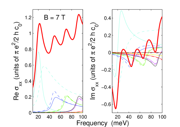
Figure 4: (Color online) The same as in Figs. 2 but at $B=$7 T.

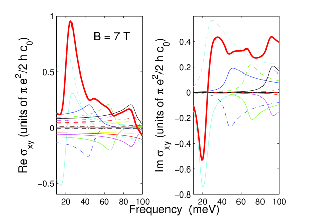
Figure 5: (Color online) Real and imaginary parts of the dynamical Hall conductivity at $B=$7 T (thick line) with the partial contributions of various electron transition are shown in the thin lines.

Let us analyze the spectroscopy of the cyclotron resonances at $B=$ 20 T. The line at 292 meV is a doublet resulted from the electron transitions $|25\rangle\rightarrow|36\rangle\,$ and $|26\rangle\rightarrow|35\rangle$ near the $K$ point of the Brillouin zone (see Fig. 1). In the similar way, the 240-meV line includes the $|24\rangle\rightarrow|35\rangle\,$ and $|25\rangle\rightarrow|34\rangle$ doublet splitted due to the electron-hole asymmetry. However, the broad line at 165 meV involves other transitions besides the similar $|23\rangle\rightarrow|34\rangle\,,$ $|24\rangle\rightarrow|33\rangle$ doublet at 184 meV. First is the transition $|11\rangle\rightarrow|10\rangle$ (161 meV) near the $H$ point. Then, the transitions $|22\rangle\rightarrow|21\rangle$ produce the broad band. The high-frequency side of the band (170 mev at $H$) and the low-frequency side (70 meV, at the intersection of the $|21\rangle-$level with the Fermi level) contribute into the 165-meV and 50-meV lines, correspondingly. The position of the broad band is very sensitive to the variation of the tight-binding parameters and to the magnetic field. The comparison of Fig. 4 to Fig. 2 shows that the $|23\rangle\rightarrow|34\rangle\,$ line does not interfere with other transitions at the weaker field. The main contribution into the sharp 50-meV line is resulted from $|21\rangle\rightarrow|32\rangle$ transitions near the $K$-point. The positions of the lines for the fields in the range of 20 – 30  T agree very well with observations of Refs. OFS ; CBN . We do not correct the positions by a variation of the tight-binding parameters. Let us emphasize that the imaginary part of the dynamical conductivity is of the order of the real part.

The optical Hall conductivity $\sigma_{xy}(\omega)$ in the ac regime is shown in Figs. 3 and 5. It is evident that the interpretation of the Faraday rotation governed by the conductivity $\sigma_{xy}(\omega)$ (see Fig. LABEL:kerrang) is much more complicated in comparison with the longitudinal conductivity. The conductivities $\sigma_{xx}(\omega)$ and $\sigma_{xy}(\omega)$ allow us to calculate the reflectivity and the Faraday rotation as functions of frequency.

Notice that the band structure shown in Fig. 1 constrains to consider the (semi)metal-insulator transition while varying the carrier concentration and applying the magnetic field. The phase transition induced by the electron-hole interaction has been discussed in Refs. KTS ; Kh ; GGM . As one can see in Fig. 1, the hole doping can decrease the Fermi energy. While the Fermi level appears between the $|22\rangle$ and $|10\rangle$ levels, the insulator arises with a gap of 34 meV. This phase transition does not involve the electron-electron interaction and it is resulted from the layered graphite structure with the small electron dispersion of the zero mode in the $k_{z}$-direction.

Author is thankful to A. Kuzmenko for discussions and corrections. This work was supported by the Russian Foundation for Basic Research (grant No. 10-02-00193-a) and by the SCOPES grant IZ73Z0$\_$128026 of the Swiss NSF. Author is grateful to the Max Planck Institute for the Physics of Complex Systems for hospitality in Dresden.

References

- (1) J.W. McClure, Phys. Rev. 108, 612 (1957); J.C. Slonczewski and P.R. Weiss, Phys. Rev. 109, 272 (1958).
- (2) G.W. Semenoff, Phys. Rev. Lett. 53, 2449 (1984).
- (3) W.W. Toy, M.S. Dresselhaus, G. Dresselhaus, Phys. Rev. B 15, 4077 (1977).
- (4) R.E. Doezema, W.R. Datars, H. Schaber, A. Van Schyndel, Phys. Rev. B 19, 4224 (1979).
- (5) Z.Q. Li, S.-W. Tsai, W.J. Padilla, S.V. Dordevic, K.S. Burch, Y.J. Wang, D.N. Basov, Phys. Rev. B 74, 195404 (2006).
- (6) M. Orlita, C. Faugeras, G. Martinez, D.K. Maude, M.L. Sadowski, M. Potemski, Phys. Rev. Lett. 100, 136403 (2008).
- (7) M. Orlita, C. Faugeras, J.M. Schneider, G. Martinez, D.K. Maude, M. Potemski, Phys. Rev. Lett. 102, 166401 (2009).
- (8) M. Orlita, M. Potemski, Semicond. Sci. Technol. 25, 063001 (2010).
- (9) I. Crassee, J. Levallois, A. L. Walter, M. Ostler, A. Bostwick, E. Rotenberg, T. Seyler, D. van der Marel, A. Kuzmenko, Nature Physics 9, 48 (2010).
- (10) Y. Kopelevich, J.H.S. Torres, R.R. da Silva, F. Mrowka, H. Kempa, P. Esquinazi, Phys. Rev. Lett. 90, 156402 (2003).
- (11) I. A. Luk’yanchuk, Y. Kopelevich, Phys. Rev. Lett. 97, 256801 (2006).
- (12) Z. Jiang, Y. Zhang, H.L. Stormer, P. Kim, Phys. Rev. Lett. 99, 106802 (2007).
- (13) J.M. Schneider, M. Orlita, M. Potemski, D.K. Maude, Phys. Rev. Lett. 102, 166403 (2009).
- (14) A.N. Ramanayaka, R. G. Mani, arXiv:1010.0603v1 (2010).
- (15) K.-C. Chuang, A.M.R. Baker, R.J. Nicholas, Phys. Rev. B 80, 161410(R) (2009).
- (16) L.A. Falkovsky, Phys. Rev. B 82, 073103 (2010).
- (17) G. Li, E.Y. Andrei, Nature Phys. 3, 623 (2007).
- (18) W.-K. Tse, A.H. MacDonald, Phys. Rev. B 82, 161104R (2010).
- (19) T. Morimoto, Y. Hatsugai, H. Aoki, Phys. Rev. Lett. 103, 116803 (2009).
- (20) M. Koshino, T. Ando, Phys. Rev. B 77, 115313 (2008).
- (21) A.A. Abrikosov, L.P. Gorkov, I.E. Dzyaloshinski, Methods of quantum field theory in statistical physics, Dover Publications, N.Y.
- (22) L.A. Falkovsky, A.A. Varlamov, Eur. Phys. J. B 56, 281 (2007).
- (23) P. Nozieres, Phys. Rev. 109, 1510 (1958).
- (24) A.B. Kuzmenko, E. van Heumen, F. Carbone, D. van der Marel, Phys. Rev. Lett. 100, 117401 (2008).
- (25) H. Suematsu, S. Tanuma, J. Phys. Soc. of Jpn. 33, 1619 (1972).
- (26) B.Partoens and F.M. Peeters, Phys. Rev. B 74, 075404 (2006).
- (27) A. Grüneis, C. Attaccalite, L. Wirtz, H. Shiozawa, R. Saito, T. Pichler, A. Rubio, Phys. Rev. B 78, 205425 (2008).
- (28) D.V. Khveshchenko, Phys. Rev. Lett. 87, 246802 (2001).
- (29) E.V. Gorbar, V.P. Gusynin, V.A. Miransky, L.A. Shovkovy, Phys. Rev. B 66, 045108 (2002).