ANALYTIC APPROACH TO PERTURBED EINSTEIN RING WITH ELLIPTICAL NFW LENS MODEL

Abstract

We investigate the validity of the approximate method to describe a strong gravitational lensing which was extended by Alard on the basis of a perturbative approach to an Einstein ring. Adopting an elliptical Navarro-Frenk-White (NFW) lens model, we demonstrate how the approximate method works, focusing on the shape of the image, the magnification, caustics, and the critical line. Simplicity of the approximate method enables us to investigate the lensing phenomena in an analytic way. We derive simple approximate formulas which characterise a lens system near the Einstein ring.

1 Introduction

Cold dark matter is one of the most important components in the universe. The cosmic microwave background anisotropies and the large scale distribution of galaxies cannot be naturally explained without the cold dark matter component. The mean density parameter of the cold dark matter has been measured precisely,[1] but its true character has not been identified. The elementary particle physics predicts possible candidates of the cold dark matter, and many experiments are ongoing aiming at a direct measurement.

The cold dark matter is considered to be distributed associated with each galaxy, forming dark matter halo. Then, the investigation of the structure of the halos is quite important in exploring the nature and the origin of the dark matter. The strong gravitational lensing is a useful probe of the halo-structure (see, e.g.,[2] for a review). Especially, a lens system near Einstein ring is useful because a wealth of information can be obtained.[3]

Besides, the strong lensing systems are also useful as a tool of the dark energy study.[4][8] Because of the recent observational developments, many strong lensing systems have been found. The strong lensing statistics is now becoming one of the powerful tool for exploring the nature of the dark energy.[9] Future dark energy surveys will detect much more strong lensing systems (see, e.g.,[10]), and the strong lensing system will play a more important roll in cosmology.

In realistic situations, the mass distribution in a halo is not simple, which makes reconstruction of the lens model complicated. The lens equation is complicated for a non-spherical lens model, which needs to be solved numerically. Then, analytic approximate approach to strong lensing system is useful, if its validity and accuracy are guaranteed. A perturbative approach to the lensing system close to the Einstein ring configuration was developed, e.g.,[11, 12]. Recently, Alard extended the perturbative approach, which is applied to analyse lensing systems.[15][18]

In the present paper, we investigate the validity of the perturbative approach to the lensing system close to an Einstein ring, assuming an elliptical lens model. We demonstrate the validity of the perturbative approach quantitatively, by comparing with an exact approach on the basis of the numerical method, focusing on the shape of the image, the magnification, the caustics, and the critical line. Using the approximate method, expanded in terms of the ellipticity parameter of the lens model, we derive simple approximate formulas which characterise an elliptical lensing system near the Einstein ring in an analytic way.

This paper is organized as follows: In section 2, we briefly review the basic formulas for the gravitational lensing and the perturbative approach to a perturbed Einstein ring, based on the work by Alard.[15, 16] In section 3, we compare the perturbative approach with the exact approach that relies on a numerical method, focusing on the shape of lensed images, the caustics, the critical curve, and the magnification, respectively. We demonstrate the validity of the perturbative approach at a quantitative level. In section 4, some useful formulas are presented, which are derived using the perturbative approach in the analytic manner. Section 5 is devoted to summary and conclusions. Throughout the paper, we use the unit in which the speed of light equals 1.

2 Basic Formulas

2.1 General basis

We briefly review basic formulas for the strong lensing (e.g.,[12]). The deflection angle of a lens object is determined by

$$\vec{\hat{\alpha}}=2\int_{0}^{\chi_{\rm S}}{\partial\Phi({\vec{\xi},\chi})\over\partial\vec{\xi}}d\chi,$$ (1)

where $\Phi$ is the gravitational potential of the lens object, $\chi$ is the radial coordinate connecting the observer and the lens object, $\vec{\xi}$ is the two dimensional vector on the lens plane, which is orthogonal to the coordinate $\chi$. The gravitational potential $\Phi$ is related to the mass density distribution of the lens $\rho({\vec{\xi},\chi})$ by the Poisson equation,

$$\triangle\Phi({\vec{\xi},\chi})=4\pi G\rho({{\vec{\xi},\chi}}),$$ (2)

where $\triangle$ denotes the 3-dimensional Laplacian, and $G$ is the gravitational constant.

Introducing the surface mass density $\Sigma(\vec{\xi})$, which is the projected mass density on the lens plane,

$$\Sigma(\vec{\xi})=\int_{0}^{\chi_{\rm S}}\rho({{\vec{\xi},\chi}})d\chi,$$ (3)

and the lensing potential,

$$\psi(\vec{\xi})=\int_{0}^{\chi_{\rm S}}\Phi({{\vec{\xi},\chi}})d\chi,$$ (4)

which are related by

$$\triangle^{(2)}\psi(\vec{\xi})=4\pi G\Sigma(\vec{\xi}),$$ (5)

where $\triangle^{(2)}$ denotes the 2-dimensional Laplacian. The solution is

$$\psi(\vec{\xi})=2G\int d^{2}\xi^{\prime}\Sigma(\vec{\xi}^{\prime})\log|\vec{\xi}-\vec{\xi}^{\prime}|+{\rm constant}.$$ (6)

Then, the deflection angle is

$$\vec{\hat{\alpha}} = 2{\partial\psi({\vec{\xi}})\over\partial\vec{\xi}}=4G\int d^{2}\xi^{\prime}\Sigma(\vec{\xi}^{\prime}){\vec{\xi}-\vec{\xi}^{\prime}\over|\vec{\xi}-\vec{\xi}^{\prime}|^{2}}.$$ (7)

Now we consider the gravitational lens equation,

$$\vec{\eta}={D_{\rm S}\over D_{\rm L}}\vec{\xi}-{D_{\rm LS}}\vec{\hat{\alpha}},$$ (8)

where $D_{\rm LS}$ is the angular diameter distance between the lens and a source object, $D_{\rm S}$ is the distance between the observer and the source, $D_{\rm L}$ is the distance between the observer and the lens, and $\vec{\eta}$ is the two dimensional vector on the source plane orthogonal to the coordinate $\chi$. Introducing a characteristic length in the lens plane, $\xi_{0}$, and $\eta_{0}=\xi_{0}D_{\rm S}/D_{\rm L}$ in the source plane, we define

$$\vec{y}=\vec{\eta}/\eta_{0}$$ (9)

$$\vec{x}=\vec{\xi}/\xi_{0},$$ (10)

then, the lens equation becomes

$$\vec{y}=\vec{x}-\nabla_{\vec{x}}\phi({\vec{x}}),$$ (11)

where we defined

$$\phi({\vec{x}})={1\over\pi}\int d^{2}x^{\prime}\kappa(\vec{x}^{\prime})\log|\vec{x}-\vec{x}^{\prime}|$$ (12)

with

$$\kappa(\vec{x})={\Sigma(\vec{\xi})\over\Sigma_{\rm cr}},$$ (13)

$$\Sigma_{\rm cr}^{-1}={4\pi GD_{\rm LS}D_{\rm L}\over D_{\rm S}}.$$ (14)

2.2 Perturbative approach to Einstein ring

Next, we review the perturbative approach to the Einstein ring developed by Alard [15, 16] (cf. [11, 12]). When the projected density of the lens $\Sigma$ is circularly symmetric and the source is located at the origin of the source plane, ${\vec{y}}=0$, an Einstein ring is formed. The radius of the Einstein ring is determined by

$$\vec{x}-{\partial\phi_{0}(|{\vec{x}}|)\over\partial\vec{x}}=0,$$ (15)

where $\phi_{0}(|\vec{x}|)$ denotes the circularly symmetric lens potential. We denote the solution of Eq. (15) by $\vec{x}=\vec{x}_{E}$. Thus, $|\vec{x}_{E}|$ is the Einstein radius. Hereafter, we use the notation $x=|\vec{x}|$ and $x_{E}=|\vec{x}_{E}|$.

We consider the perturbative approach to the Einstein ring, then assume that the deviation from the circularly symmetric lens is small. Introducing the small deviation, which are denoted by the quantities with $\delta$,

$$\vec{y}=\delta\vec{y},$$ (16)

$$\vec{x}=\vec{x}_{E}+\delta\vec{x},$$ (17)

$$\phi(\vec{x})=\phi_{0}(x)+\delta\phi({\vec{x}}),$$ (18)

the lens equation (11) is rephrased as

$$\delta\vec{y}={\vec{x}}_{E}+\delta\vec{x}-\nabla_{\vec{x}}[\phi_{0}(x)+\delta\phi({\vec{x}})]\Big{|}_{\vec{x}=\vec{x}_{E}+\delta\vec{x}}.$$ (19)

Assuming that the deviation from the circularly symmetric lens is small, we introduce the small expansion parameter $\varepsilon$. Explicitly, we assume

$$\delta\vec{y}={\cal O}(\varepsilon),$$ (20)

$$\delta\vec{x}={\cal O}(\varepsilon),$$ (21)

$$\delta\phi({\vec{x}})={\cal O}(\varepsilon).$$ (22)

We find the following lens equation at the lowest order of $\varepsilon$,

$$\delta\vec{y}=\delta\vec{x}-[(\delta\vec{x}\cdot\nabla_{\vec{x}})\nabla_{\vec{x}}\phi_{0}(x)+\nabla_{\vec{x}}\delta\phi({\vec{x}})]\Big{|}_{\vec{x}=\vec{x}_{E}},$$ (23)

where we used Eq. (15).

We consider a circular source with the radius $\delta r_{s}$, whose centre is located at the coordinate $(\delta y_{10},\delta y_{20})$ on the source plane. Then, the circumferences of the source is parameterised as

$$\delta y_{1}=\delta y_{10}+\delta r_{s}\cos\varphi$$ (24)

$$\delta y_{2}=\delta y_{20}+\delta r_{s}\sin\varphi$$ (25)

with the parameter $\varphi$ in the range $0\leq\varphi\leq 2\pi$, where we assume that $\delta y_{10}$, $\delta y_{20}$ and $\delta r_{s}$ are the quantities of the order of $\varepsilon$. Similarly, we may rewrite the image position $\vec{x}=\vec{x}_{E}+\delta\vec{x}$ as [15]

$$x_{1}=(x_{E}+\delta x)\cos\theta,$$ (26)

$$x_{2}=(x_{E}+\delta x)\sin\theta.$$ (27)

Here, we don’t need to consider the perturbation of $\theta$ because of the symmetry of the un-perturbed image.[15] In the un-perturbed situation, the image of a point source is a circle, and there are an infinite number of the image at any $\theta$. Then, at any angular position of the perturbed point, there is always an un-perturbed point at the same angular position on the circle.

The lens equation (23) yields

$$\delta y_{10}+\delta r_{s}\cos\varphi=\bigl{[}\delta x\cos\theta\left(1-\partial_{x}^{2}\phi_{0}(x)\right)$$

$$~{}~{}~{}~{}~{}-\cos\theta\partial_{x}\delta\phi(x,\theta)+{\sin\theta\over x}\partial_{\theta}\delta\phi(x,\theta)\bigr{]}\Big{|}_{x=x_{E}},$$ (28)

$$\delta y_{20}+\delta r_{s}\sin\varphi=\bigl{[}\delta x\sin\theta\left(1-\partial_{x}^{2}\phi_{0}(x)\right)$$

$$~{}~{}~{}~{}~{}-\sin\theta\partial_{x}\delta\phi(x,\theta)-{\cos\theta\over x}\partial_{\theta}\delta\phi(x,\theta)\bigr{]}\Big{|}_{x=x_{E}}.$$ (29)

Combining these equations, we have

$$\delta x={1\over(1-\partial_{x}^{2}\phi_{0}(x))}\Bigl{[}\partial_{x}\delta\phi(x,\theta)+\delta y_{10}\cos\theta+\delta y_{20}\sin\theta\pm\sqrt{\Delta^{2}(x,\theta)}\Bigr{]}\Bigr{|}_{x=x_{E}},$$

(30)

where we defined

$$\Delta^{2}(x,\theta)=\delta r_{s}^{2}-\Bigl{(}{1\over x}\partial_{\theta}\delta\phi(x,\theta)-\delta y_{10}\sin\theta+\delta y_{20}\cos\theta\Bigr{)}^{2}.$$ (31)

This is the formula derived by Alard.[15, 16]

For comparison, we summarised the corresponding formula without the perturbative approximation in the appendix A. One can derive Eq. (30) from Eq. (111).

2.3 Perturbative NFW lens model

A mass model commonly used for strong lensing is based on high-resolution numerical simulations of dark-matter halos in the $\Lambda$CDM framework by Navarro, Frenk and White (1996, 1997; hereafter NFW[13, 14]), in which the density profile is parameterised by the scale radius $r_{s}$ and the constant $\rho_{s}$,

$$\rho(R)=\frac{\rho_{s}}{\left(R/r_{s}\right)\left(1+R/r_{s}\right)^{2}},$$ (32)

where $R=\sqrt{\xi^{2}+\chi^{2}}$ is the 3-dimensional length. Choosing $r_{s}=\xi_{0}$, the lens potential becomes [20]

$$\phi_{\rm NFW}(x)=4\kappa_{s}F(x),$$ (33)

where we defined

$$F(x)={1\over 2}\log^{2}\frac{x}{2}+\left\{\begin{array}[]{cc}+2\arctan^{2}\sqrt{\frac{x-1}{x+1}}&(x>1)\\ -2{\rm arctanh}^{2}\sqrt{\frac{1-x}{1+x}}&(x<1)\\ \log x&(x=1)\end{array}\right.$$ (37)

and

$$\kappa_{s}={\rho_{s}\xi_{0}\over\Sigma_{\rm cr}}.$$ (38)

We denote the solution of the lens equation for the circular NFW lens model by $u_{0}$, which satisfies

$$u_{0}={\partial\over\partial u_{0}}\phi_{\rm NFW}(u_{0}).$$ (39)

In the present paper, for an asymmetric lens model, we adopt the potential

$$\phi({\vec{x}})=\phi_{\rm NFW}\left(x\sqrt{1-\eta\cos 2\theta}\right).$$ (40)

Instead of $\vec{x}$ and $\vec{y}$, we introduce $\vec{\widetilde{x}}$ and $\vec{\widetilde{y}}$, which is normalised by the Einstein radius $u_{0}$ defined with Eq. (39),

$$\vec{x}=u_{0}\vec{\widetilde{x}},$$ (41)

$$\vec{y}=u_{0}\vec{\widetilde{y}}.$$ (42)

Then, the lens equation is rewritten

$$\vec{\widetilde{y}}=\vec{\widetilde{x}}-\nabla_{\vec{\tilde{x}}}{\widetilde{\phi}}$$ (43)

with

$${\widetilde{\phi}}={4\kappa_{s}\over u_{0}^{2}}F\left(u_{0}{\widetilde{x}}\sqrt{1-\eta\cos 2\theta}\right),$$ (44)

where ${\widetilde{x}}=|\vec{\widetilde{x}}|$, $F(x)$ is defined by Eq. (37), and

$$\left({4\kappa_{s}\over u_{0}^{2}}\right)^{-1}=\log\frac{u_{0}}{2}+\left\{\begin{array}[]{cc}{2\over\sqrt{u_{0}^{2}-1}}\arctan\sqrt{\frac{u_{0}-1}{u_{0}+1}}&(u_{0}>1)\\ {2\over\sqrt{1-u_{0}^{2}}}{\rm arctanh}\sqrt{\frac{1-u_{0}}{1+u_{0}}}&(u_{0}<1)\\ 1&(u_{0}=1)\end{array}\right.$$ (48)

Finally, the potential of the elliptical NFW lens is written as

$$\widetilde{\phi}=\widetilde{\phi}_{0}(\widetilde{x})+\widetilde{\delta\phi}(\widetilde{x},\theta)$$ (49)

with

$$\widetilde{\phi}_{0}(\widetilde{x})={4\kappa_{s}\over u_{0}^{2}}F(u_{0}\widetilde{x}),$$ (50)

$$\widetilde{\delta\phi}(\widetilde{x},\theta)={4\kappa_{s}\over u_{0}^{2}}\Bigl{(}F\bigl{(}u_{0}\widetilde{x}\sqrt{1-\eta\cos 2\theta}\bigr{)}-F(u_{0}\widetilde{x})\Bigr{)}.$$ (51)

In the appendixes A and B, useful formulas related with the elliptical NFW lens potential are summarized. In these appendixes, only the case $u_{0}\widetilde{x}\sqrt{1-\eta\cos 2\theta}<1$ is described, but the case $u_{0}\widetilde{x}\sqrt{1-\eta\cos 2\theta}>1$ is obtained by the analytic continuation.

3 Validity of the Perturbative approach

We here investigate the validity of the perturbative approach, comparing with results without any approximation. For being definite, we consider the following three cases.

(a) Exact approach without any approximation.

(b) Perturbative approach described in the previous section.

(c) Approximate approach: the perturbative approach (b) plus the lowest-order expansion of $\eta$ (See also the appendix C).

3.1 Image

We consider the lensed image of the circumference of the circular source, whose center is located at $(\widetilde{\delta y_{10}},\widetilde{\delta y_{20}})$. The source’s radius is $\widetilde{\delta r_{s}}$. In the exact approach (a), the circumference of the lensed image is obtained by solving Eq. (111), which is derived in the appendix A. Eq. (111) can be solved with an iterative method numerically. On the other hand, in the perturbative approach (b), the circumference follows Eq. (30), which is equivalent to

$$\widetilde{\delta x}={1\over(1-\partial_{\tilde{x}}^{2}\widetilde{\phi_{0}}(\widetilde{x}))}\Bigl{[}\partial_{\widetilde{x}}\widetilde{\delta\phi}(\widetilde{x},\theta)+\widetilde{\delta y_{10}}\cos\theta+\widetilde{\delta y_{20}}\sin\theta\pm\sqrt{\widetilde{\Delta}^{2}(\widetilde{x},\theta)}\Bigr{]}\Bigr{|}_{\widetilde{x}=1},$$

(52)

with

$$\widetilde{\Delta}^{2}(\widetilde{x},\theta)=\widetilde{\delta r_{s}}^{2}-\Bigl{(}{1\over\widetilde{x}}\partial_{\theta}\widetilde{\delta\phi}(\widetilde{x},\theta)-\widetilde{\delta y_{10}}\sin\theta+\widetilde{\delta y_{20}}\cos\theta\Bigr{)}^{2}.$$ (53)

Eqs. (52) and (53) are the same as Eq. (12) in the reference Alard [15]. In the approximate approach (b), we use Eqs. (119)$\sim$(121) to find the solution, Eq. (52). In the approximate approach (c), we use the quantities of the lowest-order of $\eta$, given by Eqs. (124) and (125), instead of Eqs. (120) and (121).

The upper left panels of Fig. 1 show the lensed image. (a) is the exact approach, (b) is the perturbative approach, and (c) is the approximate approach, respectively. The panel (d) plots these three approaches for comparison. Here we adopted the parameters $\widetilde{\delta r_{s}}=0.07$, $\widetilde{\delta y_{10}}=0.09$, $\widetilde{\delta y_{20}}=0$, $\eta=0.15$ and $u_{0}=0.5$. In this case, the lens effect splits the image into four. The dashed circle in each panel is the Einstein radius of a point source.

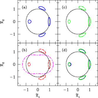
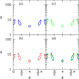
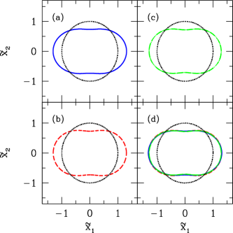
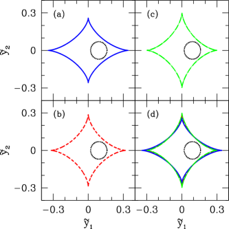
Figure 1: Comparison of the three approaches, (a) exact approach, (b) perturbative approach and (c) approximate approach of the lowest-order of the expansion of $\eta$. The panel labelled by (a), (b) and (c) corresponds to the approach (a), (b) and (c), respectively, while (d) plots all the three approaches for comparison. The upper left panels show the lensed image of the circumference of a circular source. The dotted circle is the Einstein ring. The long and short dashed curve is the critical line. The parameters $\widetilde{\delta r_{s}}=0.07$, $\widetilde{\delta y_{10}}=0.09$, $\widetilde{\delta y_{20}}=0$, $\eta=0.15$ and $u_{0}=0.5$. This is type I. The upper right panels show the magnification factor $\mu$ on the circumference of the images as a function of the angular coordinate of the image plane. The lower left panels show the critical line. The dotted circles are the Einstein ring. The lower right panels show the caustics on the lens plane. The circle is the circumference of source.

3.2 Magnification factor

The magnification factor due to the gravitational lensing is given by the inverse of the determinant of the Jacobian matrix,[12]

$$\mu=|J|^{-1}=\biggl{|}{\rm det}{\partial\vec{y}\over\partial\vec{x}}\biggr{|}^{-1}.$$ (54)

For a general lens potential, the determinant of the Jacobian matrix can be written as

$$J={1\over\widetilde{x}}\biggl{[}\Bigl{(}1-{\partial^{2}\widetilde{\phi}\over\partial{\tilde{x}}^{2}}\Bigr{)}\Bigl{(}\widetilde{x}-{\partial\widetilde{\phi}\over\partial\tilde{x}}-{1\over\widetilde{x}}{\partial^{2}\widetilde{\phi}\over\partial\theta^{2}}\Bigr{)}-{1\over\widetilde{x}}\Bigl{(}{1\over\widetilde{x}}{\partial\widetilde{\phi}\over\partial\theta}-{\partial^{2}\widetilde{\phi}\over\partial\tilde{x}\partial\theta}\Bigr{)}^{2}\biggr{]},$$ (55)

where we used Eqs. (114)$\sim$(118). This is the exact approach (a) for the magnification.

On the other hand, in the case of the perturbative approach (b), we have

$$J=\Bigl{(}1-{\partial^{2}\widetilde{\phi}_{0}\over\partial\tilde{x}^{2}}\Bigr{)}\times\Bigl{(}\widetilde{\delta x}-\widetilde{\delta x}{\partial^{2}\widetilde{\phi}_{0}\over\partial\tilde{x}^{2}}-{\partial\widetilde{\delta\phi}\over\partial\tilde{x}}-{\partial^{2}\widetilde{\delta\phi}\over\partial\theta^{2}}\Bigr{)}\Bigr{|}_{\widetilde{x}=1},$$ (56)

where we used the condition of the Einstein ring. $\partial\widetilde{\phi}_{0}/\partial\tilde{x}|_{\widetilde{x}=1}=1$. Note that $\widetilde{\phi}(\widetilde{x},\theta)=\widetilde{\phi}_{0}(\widetilde{x})+\widetilde{\delta\phi}(\widetilde{x},\theta)$ and $\widetilde{x}=1+\widetilde{\delta x}$. The formulas (119) $\sim$(122) are used for the perturbative approach (b), and (124)$\sim$(126) for the approximate approach (c), respectively.

The upper right panels (a)$\sim$(d) of Fig. 1 show the magnification of the circumference of lensed image as a function of the angular coordinate of the image plane. The panels (a)$\sim$(c) correspond to the three approaches (a)$\sim$(c), respectively. The panel (d) plots the three approaches. The model parameters are the same as those of the upper left panels for the lensed image.

3.3 Critical line

The definition of the critical curve is $J=0$ on the image plane. In the exact approach (a), we solve

$$\widetilde{x}={\partial\widetilde{\phi}\over\partial\tilde{x}}+{1\over\widetilde{x}}{\partial^{2}\widetilde{\phi}\over\partial\theta^{2}}+{1\over\widetilde{x}}\Bigl{(}1-{\partial^{2}\widetilde{\phi}\over\partial{\tilde{x}}^{2}}\Bigr{)}^{-1}\Bigl{(}{1\over\widetilde{x}}{\partial\widetilde{\phi}\over\partial\theta}-{\partial^{2}\widetilde{\phi}\over\partial\tilde{x}\partial\theta}\Bigr{)}^{2},$$ (57)

which is obtained using Eq. (55).

In the perturbative approach (b), the critical line is

$$\widetilde{\delta x}={1\over 1-\partial^{2}\widetilde{\phi_{0}}/\partial\tilde{x}^{2}}\left({\partial\widetilde{\delta\phi}\over\partial\tilde{x}}+{\partial^{2}\widetilde{\delta\phi}\over\partial\theta^{2}}\right)\biggr{|}_{\widetilde{x}=1},$$ (58)

from $J=0$ with Eq. (56). This equation is the same as Eq. (30) in the reference by Alard [15]. In the perturbative approach (b), we use Eqs. (120) and (122), while we use Eqs. (124) and (126) in the approximate approach (c).

The lower left panels (a)$\sim$(d) of Fig. 1 show the critical line (solid curve) on the image plane. The panels (a)$\sim$(c) correspond to the three approaches (a)$\sim$(c), respectively, and the panel (d) plots the three approaches. The dotted circle is the Einstein ring. The model parameters are the same as those of the other panels of Fig. 1.

3.4 Caustics

The caustics are defined by $J=0$ on the source plane, which can be mapped from the critical line on the image plane by the lens equation. The caustics are important in understanding the nature of deformation of an Einstein ring.

In the exact approach (a), the caustics are obtained by substituting the solution of Eq. (57) into (109) and (110).

In the perturbative approach (b), the caustics are given by

$$\widetilde{\delta y_{1}}={\partial^{2}\widetilde{\delta\phi}\over\partial\theta^{2}}\bigg{|}_{\widetilde{x}=1}\cos\theta+{\partial\widetilde{\delta\phi}\over\partial\theta}\bigg{|}_{\widetilde{x}=1}\sin\theta,$$ (59)

$$\widetilde{\delta y_{2}}={\partial^{2}\widetilde{\delta\phi}\over\partial\theta^{2}}\bigg{|}_{\widetilde{x}=1}\sin\theta-{\partial\widetilde{\delta\phi}\over\partial\theta}\bigg{|}_{\widetilde{x}=1}\cos\theta,$$ (60)

which are obtained by substituting Eq.(58) into the lens equation (28) and (29). Eqs. (59) and (60) are the same as Eq. (31) in the reference by Alard[15], where $x_{s}$ and $y_{s}$ are used instead of $\widetilde{\delta y_{1}}$ and $\widetilde{\delta y_{2}}$, respectively. In the approximate approach (c), we use (125) and (126).

The lower right panels (a)$\sim$(d) of Fig. 1 show the caustics (solid curves) on the source plane. The panels (a)$\sim$(c) correspond to the three approaches (a)$\sim$(c), respectively, and the panel (d) plots all three approaches. The spherical circles are the circumference of the source. The model parameters are the same as those of the other panels of Fig. 1.

3.5 Typical configurations

In Fig. 1, we adopted the parameters $\widetilde{\delta r_{s}}=0.07$, $\widetilde{\delta y_{10}}=0.09$, $\widetilde{\delta y_{20}}=0$, $\eta=0.15$ and $u_{0}=0.5$. Figs. 2 and 3 are the same as Fig. 1 but with $\eta=0.1274$ and $\eta=0.08$, respectively, instead of $\eta=0.15$. The other parameters are the same as those of Fig. 1, then the source configuration of Figs. 1, 2, and 3 are the same. As $\eta$ becomes smaller, the size of the caustics becomes smaller, and the shape of the critical line becomes more spherical. Also, as $\eta$ becomes smaller, the right-side three separated images become to merge. Fig. 2 is the critical configuration when the merger occurs. One can observe that the merger occurs when the circumference of the source contacts with the caustics. In the upper right panels of Figs. 2 and 3, the large enhancement of the magnification appears. This reflects the facts that the magnification diverges when a source is on the caustics and when the image crosses the critical line. Figs. 1, 2 and 3 represent typical types of lensed image, which we call type I, II and III, respectively.

As $\eta$ becomes smaller furthermore, the left-side image and the right-side image become elongated, and form a ring, as is demonstrated in Figs. 4 and 5. The parameters of Fig. 4 are $\widetilde{\delta r_{s}}=0.07$, $\widetilde{\delta y_{10}}=0.06$, $\widetilde{\delta y_{20}}=0$, $\eta=0.0205$ and $u_{0}=0.5$. Fig. 5 is the same as Fig. 4 but with the different value of $\eta=0.011$, instead of $\eta=0.0205$. These two images are almost rings, i.e., Einstein rings with finite width. Fig. 4 is the critical configuration when a ring is formed. Figs. 4 and 5 represent typical types of lensed image of a ring, which we call type IV and V, respectively. In these cases, the size of the caustics is smaller than the source size, which is clearly shown in Figs. 4 and 5. We note that the critical configuration, type IV, appears when the circumference of the source comes in contact with the caustics at the left-side caustic. The divergence of the magnification appears when the source overlaps the caustics and when the image crosses the critical line.

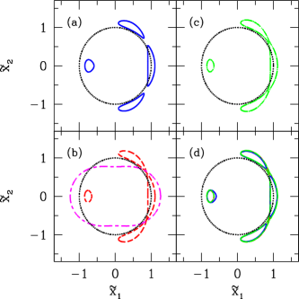
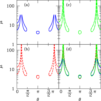
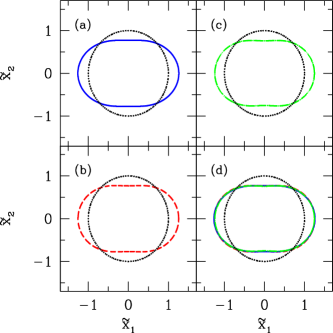
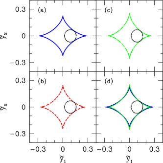
Figure 2: Same as Fig. 1 but with the parameters $\widetilde{\delta r_{s}}=0.07$, $\widetilde{\delta y_{10}}=0.09$, $\widetilde{\delta y_{20}}=0$, $\eta=0.1274$ and $u_{0}=0.5$. This is type II.

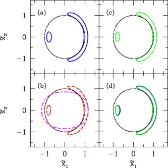
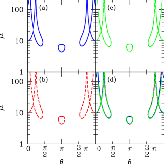
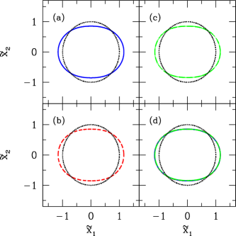
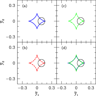
Figure 3: Same as Fig. 1 but with the parameters $\widetilde{\delta r_{s}}=0.07$, $\widetilde{\delta y_{10}}=0.09$, $\widetilde{\delta y_{20}}=0$, $\eta=0.08$ and $u_{0}=0.5$. This is type III.

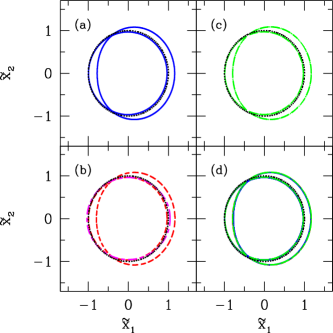
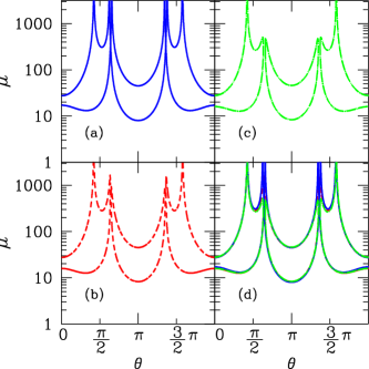
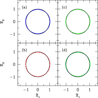
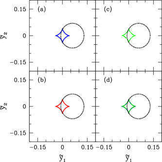
Figure 4: Same as Fig. 1 but with the parameters $\widetilde{\delta r_{s}}=0.07$, $\widetilde{\delta y_{10}}=0.06$, $\widetilde{\delta y_{20}}=0$, $\eta=0.0205$ and $u_{0}=0.5$. This is type IV.

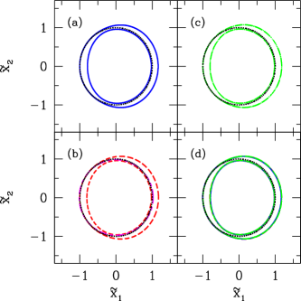
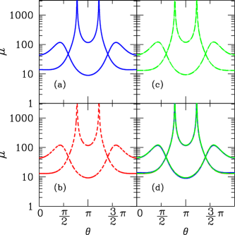
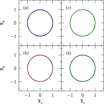
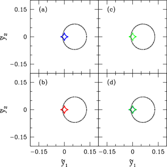
Figure 5: Same as Fig. 1 but with the parameters $\widetilde{\delta r_{s}}=0.07$, $\widetilde{\delta y_{10}}=0.06$, $\widetilde{\delta y_{20}}=0$, $\eta=0.011$ and $u_{0}=0.5$. This is type V.

3.6 Validity of the perturbative approximation

Let us discuss about the validity of the perturbative approach comparing with the exact approach. Fig. 6 plots the outer position of the image at $\theta=0$, i.e., $\widetilde{x}(\theta=0)$, as a function of $\eta$. (See also Fig. 7.) The curves labelled by (a), (b) and (c) correspond to the three approaches. In the exact approach (a), $\widetilde{x}(\theta=0)$ is given by solving Eq. (111). In the perturbative approach (b) and the approximate approach (c), $\widetilde{x}(\theta=0)=1+\widetilde{\delta x}(\theta=0)$, where $\widetilde{\delta x}(\theta=0)$ is given from Eq. (52) with the formulas in the appendix B and in the appendix C, respectively. We are considering the circumference of a circular source, and $\widetilde{x}(\theta=0)$ has the two solutions, which correspond to the two solutions of the sign $\pm$ in Eq. (111) in the exact approach (a) and Eq. (52) in the approaches (b) and (c). Fig. 6 plots the outer solution, which corresponds to the solution of the sign $+$ in Eqs. (111) and (52). In the limit, $\eta\rightarrow 0$, (b) is equivalent to (c). The difference between (a) and (b) (or (c)) in the limit $\eta\rightarrow 0$, comes from a limitation of the perturbative method. As one can see from Fig. 6, the difference between (a) and (b) becomes large for $\eta\lower 2.15277pt\hbox{$\;\buildrel>\over{\sim}\;$}0.5$, where the perturbative approach breaks down. The similar result was obtained in Figure 1 in reference by Alard (2007) [15]. Besides comparing $\widetilde{x}(\theta=0)$, it is useful to compare the position of the image edge as examined in Fig. 8 in the below (See also the reference by Peirani, et al.(2008)[19]).

Next, let us focus on the critical configurations where the number of the images changes. Four images of the type I change to two images of the type III as $\eta$ becomes smaller. The type II is the critical configuration. The two images of the type III changes to a ring configuration of the type V as $\eta$ becomes smaller. The type IV is also the critical configuration. Fig. 8 examines these critical behaviours. Fig. 8 shows the angles of the edge of the image, $\theta_{1}$, $\theta_{2}$ and $\theta_{3}$, which are defined using Fig. 7, as a function of $\eta$. In each panel, we plot $\theta_{1}$, $\theta_{2}$ and $\theta_{3}$, and the top curve is $\theta_{3}$. As $\eta$ becomes small, $\theta_{2}$ and $\theta_{1}$ merge, when the critical configuration (type II) appears. We refer $\eta_{\rm II}$ as the critical value of $\eta$ when $\theta_{2}$ and $\theta_{1}$ merge. For $\eta<\eta_{\rm II}$, we have no solution for $\theta_{1}$ and $\theta_{2}$, In the upper left panel of Fig. 8, the vertical dashed line labelled by I, II and III, are the value of $\eta$, adopted in Fig. 1, 2 and  3, respectively. The solid curve is the exact approach (a), the dashed curve is the perturbative approach (b), and the long dash-dotted curve is the approximate approach (c). Note that the three approaches (a), (b) and (c) agree very well.

The upper right panel of Fig. 8 is the same as the upper left panel, but with $\widetilde{\delta y_{10}}=0.06$, instead of $\widetilde{\delta y_{10}}=0.09$. Similarly, the lower left (right) panel is the same as the upper left panel, but with $\widetilde{\delta y_{10}}=0.15$ ($\widetilde{\delta y_{10}}=0.3$). Thus, the agreement between the three approaches is better for smaller values of $\widetilde{\delta y_{10}}$. Note also that the critical value $\eta_{\rm II}$ becomes larger as $\widetilde{\delta y_{10}}$ becomes larger.

In the upper right panel of Fig. 8, the vertical dashed line labelled by IV and V, is the value of $\eta$, adopted in Figs. 4 and  5, respectively. In this panel, $\theta_{3}$ increases as $\eta$ becomes small. We define $\eta_{\rm IV}$ by the smallest value of $\eta$ with which we can find the solution of $\theta_{3}$. The type IV critical configuration appears at $\eta=\eta_{\rm IV}$. as shown by the vertical dashed line labelled by IV. The critical configuration of type IV appears only in the upper right panel of Fig. 8, where a ring image appears for $\eta<\eta_{\rm IV}$.

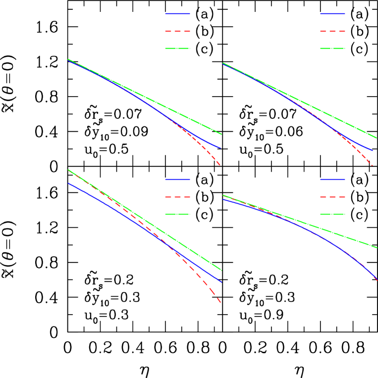
Figure 6: Comparison of the solution of the lens equation $\widetilde{x}(\theta=0)$ as a function of $\eta$. The solid curve is the exact approach (a), the dashed curve is the perturbative approach (b), and the long dash-dotted curve is the approximate approach (c). The upper left panel adopted $\widetilde{\delta r_{s}}=0.07$, $\widetilde{\delta y_{10}}=0.09$, $\widetilde{\delta y_{20}}=0$ and $u_{0}=0.5$. The upper right panel is the same as the upper left panel but with the different value of $\widetilde{\delta y_{10}}=0.09$. The lower left (right) is $\widetilde{\delta r_{s}}=0.2$ $\widetilde{\delta y_{10}}=0.3$, $u_{0}=0.3$ ($u_{0}=0.9$).

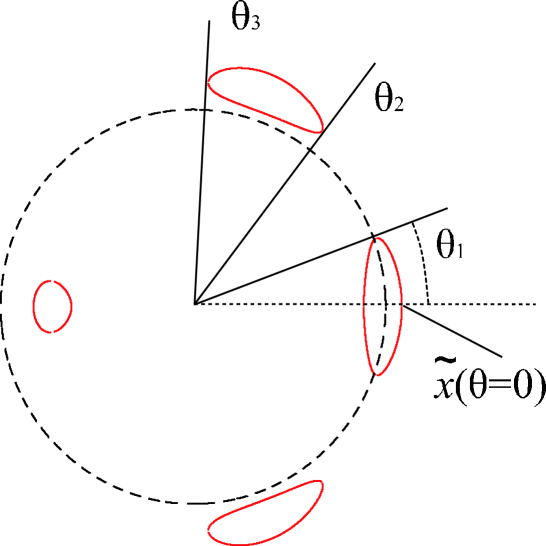
Figure 7: Definition of the angles $\theta_{1}$, $\theta_{2}$, and $\theta_{3}$, for the image of type I.

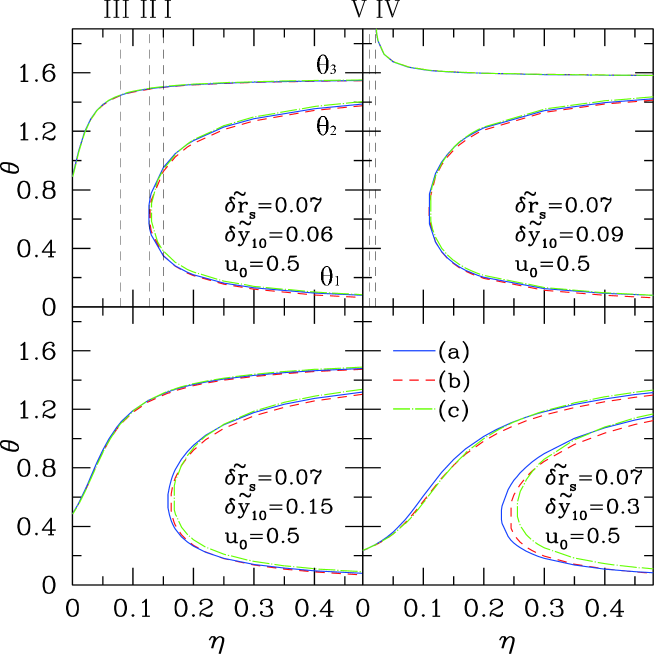
Figure 8: $\theta_{1}$, $\theta_{2}$ and $\theta_{3}$ as a function of $\eta$. In each panel, the top curve is $\theta_{3}$. As $\eta$ becomes small, $\theta_{1}$ and $\theta_{2}$ merge, when the critical configuration (type II) appears. The solid curve is the exact approach (a), the dashed curve is the perturbative approach (b), and the long dash-dotted curve is the approximate approach (c). The dashed vertical lines are the values of $\eta$ adopted in Figs. 1$\sim$5, as labelled in this figure. In this figure we adopt $\widetilde{\delta r_{s}}=0.07$, $\widetilde{\delta y_{20}}=0$ and $u_{0}=0.5$, and $\widetilde{\delta y_{10}}=0.09$ (upper left panel); $\widetilde{\delta y_{10}}=0.06$ (upper right panel); $\widetilde{\delta y_{10}}=0.15$ (lower left panel); $\widetilde{\delta y_{10}}=0.3$ (lower right panel).

4 Discussions

As is demonstrated in the above, the approximate approach (c) is not so bad. An advantage of the approximate approach (c) is that the simplicity enables us to investigate the lensing phenomena in an analytic way, as we will show in this section.

4.1 Condition of the critical configurations

First, we consider the condition that the critical configuration of type II appears, which is the transition point that the number of the images changes from four to two.

In the perturbative approach, the condition $\Delta^{2}(x_{E},\theta)\geq 0$ must be satisfied for the existence of the solution of the lens equation (see Eqs. (30) and (31)). In the approximate approach (c), from Eqs. (53) and (125), we have

$${\widetilde{\Delta}}^{2}(\widetilde{x}=1,\theta)=\widetilde{\delta r_{s}}^{2}-(\eta\sin 2\theta-\widetilde{\delta y_{10}}\sin\theta)^{2},$$ (61)

where we used $\widetilde{\delta y_{20}}=0$. Fig. 9 plots ${\widetilde{\Delta}}^{2}(\widetilde{x}=1,\theta)$ as a function of $\theta$ for the five typical cases, I $\sim$ V, corresponding to Figs. 1 $\sim$ 5. Note that our models satisfy ${\widetilde{\Delta}}^{2}(\widetilde{x}=1,\theta)={\widetilde{\Delta}}^{2}(\widetilde{x}=1,2\pi-\theta)$. Fig. 9 only plots the range of $0\leq\theta\leq\pi$. Lensed image appears under the condition ${\widetilde{\Delta}}^{2}(\widetilde{x}=1,\theta)\geq 0$. The number of separated regions with ${\widetilde{\Delta}}^{2}(\widetilde{x}=1,\theta)\geq 0$ determines the number of the images. Also the zero points of ${\widetilde{\Delta}}^{2}(\widetilde{x}=1,\theta)=0$ in the panel (I) of Fig. 9 correspond to $\theta_{1}$, $\theta_{2}$ and $\theta_{3}$ in Fig. 7.

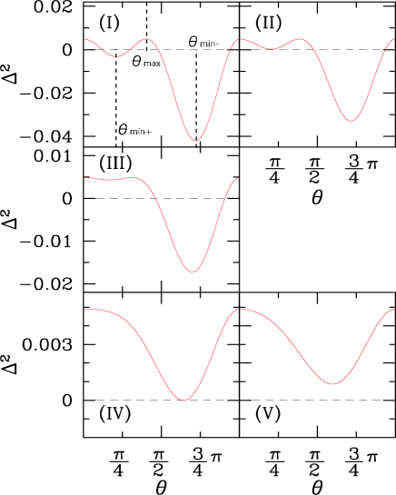
Figure 9: ${\widetilde{\Delta}}^{2}(\widetilde{x}=1,\theta)$ as a function of $\theta$ (see Eq. (61)). Here the parameters of each panel (I) $\sim$ (V) are the same as those of Figs. 1 $\sim$  5, respectively.

Let us first explain the local minimum and maximum points of ${\widetilde{\Delta}}^{2}(\widetilde{x}=1,\theta)$, $\theta_{\rm min\pm}$ and $\theta_{\rm max}$, respectively, (see the upper left panel of Fig. 9). From (61), we have,

$${d\over d\theta}{\widetilde{\Delta}}^{2}(\widetilde{x}=1,\theta) = \sin\theta[-16\eta^{2}\cos^{3}\theta+12\eta\widetilde{\delta y_{10}}\cos^{2}\theta$$ (62)

$$+(8\eta^{2}-2\widetilde{\delta y_{10}}^{2})\cos\theta-4\eta\widetilde{\delta y_{10}}]$$

$$= -16\eta^{2}\sin\theta\left(\cos\theta-{\widetilde{\delta y_{10}}\over 2\eta}\right)$$

$$\times\left(\cos\theta-{\widetilde{\delta y_{10}}+\sqrt{32\eta^{2}+\widetilde{\delta y_{10}}^{2}}\over 8\eta}\right)$$

$$\times\left(\cos\theta-{\widetilde{\delta y_{10}}-\sqrt{32\eta^{2}+\widetilde{\delta y_{10}}^{2}}\over 8\eta}\right).$$

We find that ${\widetilde{\Delta}}^{2}(\widetilde{x}=1,\theta)$ has a local maximum in the range of $0<\theta<\pi$ at

$$\cos\theta_{\rm max}={\widetilde{\delta y_{10}}\over 2\eta}{},$$ (63)

and the two local minimum at

$$\cos\theta_{\rm min\pm}={1\over 8\eta}\left(\widetilde{\delta y_{10}}\pm\sqrt{32\eta^{2}+\widetilde{\delta y_{10}}^{2}}\right).$$ (64)

The values of the local maximum and minimum are

$${\widetilde{\Delta}}^{2}(\widetilde{x}=1,\theta=\theta_{\rm max})={\widetilde{\delta r_{s}}}^{2}$$ (65)

and

$${\widetilde{\Delta}}^{2}(\widetilde{x}=1,\theta=\theta_{\rm min\pm})$$

$$~{}~{}={1\over 128\eta^{2}}\bigg{[}{\widetilde{\delta y_{10}}}^{4}-80{\widetilde{\delta y_{10}}}^{2}\eta^{2}-128\eta^{4}\pm{\widetilde{\delta y_{10}}}^{3}\sqrt{32\eta^{2}+{\widetilde{\delta y_{10}}}^{2}}$$

$$~{}~{}\pm 32\eta^{2}{\widetilde{\delta y_{10}}}\sqrt{32\eta^{2}+{\widetilde{\delta y_{10}}}^{2}}+128{\widetilde{\delta r_{s}}}^{2}\eta^{2}\bigg{]}\equiv{\widetilde{\Delta}}^{2}_{\pm},$$ (66)

respectively.

Furthermore, ${\widetilde{\Delta}}^{2}(\widetilde{x}=1,\theta)$ also has other local maximum at $\theta=0$ and $\theta=\pi$. From (61), we have

$${\widetilde{\Delta}}^{2}(\widetilde{x}=1,\theta=0)={\widetilde{\Delta}}^{2}(\widetilde{x}=1,\theta=\pi)={\widetilde{\delta r_{s}}}^{2}.$$ (67)

This means that the thickness of the arcs is approximately determined by $\widetilde{\delta r_{s}}$, which can be seen in Figs. 1$\sim$ 5.

Note that the critical configuration type II (IV) appears when ${\widetilde{\Delta}}^{2}_{+}=0$ (${\widetilde{\Delta}}^{2}_{-}=0$). From Eq. (66), the condition ${\widetilde{\Delta}}^{2}_{\pm}=0$ is rephrased as

$$f^{\pm}(\xi)=-8\left({\widetilde{\delta r_{s}}\over\eta}\right)^{2},$$ (68)

where we defined

$$f^{\pm}(\xi)=\xi^{4}-20\xi^{2}-8\pm\xi^{3}\sqrt{8+\xi^{2}}\pm 8\xi\sqrt{8+\xi^{2}},$$ (69)

and $\xi=\widetilde{\delta y_{10}}/2\eta$. Fig. 10 plots $f^{+}(\xi)$ and $f^{-}(\xi)$ as a function of $\xi$. Note that $f^{\pm}(0)=-8$. From Fig. 10, one finds $f^{+}(\xi)\geq f^{-}(\xi)$. This means that ${\widetilde{\Delta}}^{2}_{+}\geq{\widetilde{\Delta}}^{2}_{-}$, which can be proved explicitly. This also means that the configuration type always changes as ${\rm V}\rightarrow{\rm IV}\rightarrow{\rm III}\rightarrow{\rm II}\rightarrow{\rm I}$, as ${\widetilde{\delta y_{10}}/\eta}$ changes from infinity to $0$.

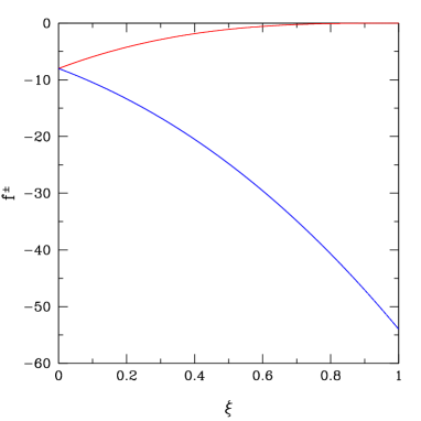
Figure 10: $f^{+}$ (upper curve) and $f^{-}$ (lower curve) as a function of $\xi$.

We can easily find the critical condition that the type II appears in an analytic way, as follows. The condition is ${\widetilde{\Delta}}^{2}_{+}=0$, i.e., Eq. (68) of the $+$ sign, which has a solution around $\xi\sim 1$ for $\eta\sim\widetilde{\delta y_{10}}$. By expanding $f^{+}(\xi)$ around $\xi=1$, we have

$$f^{+}(\xi)\simeq\frac{256}{27}(\xi-1)^{3}+\mathcal{O}(\xi-1)^{4}.$$ (70)

With this approximation, ${\widetilde{\Delta}}^{2}_{+}=0$ yields

$${\widetilde{\delta y_{10}}\over 2\eta}=1-\frac{3}{2}\left(\frac{\widetilde{\delta r_{s}}}{2\eta}\right)^{2/3}.$$ (71)

Fig. 11 is the diagram to show where the typical configurations appear on the $\eta-\widetilde{\delta y_{10}}$ plane. On the boundary between I and III, the critical configuration type II appears, while the type IV appears on the boundary between III and V. The dashed curves satisfy $\widetilde{\Delta}^{2}_{+}=0$, the dot-dashed curves satisfy $\widetilde{\Delta}^{2}_{-}=0$, which are obtained by solving Eq. (68) of the sign $+$ and $-$, respectively. The solid curves plot Eq. (71). The agreement between the dashed curve and the solid curve means the validity of the approximate formula of (71). Here, we adopted $\widetilde{\delta r_{s}}=0.07$, $u_{0}=0.5$ (upper-left panel) and $\widetilde{\delta r_{s}}=0.2$, $u_{0}=0.3$ (upper-right panel), respectively. The lower left (right) panel assumes $u_{0}=0.5$ ($u_{0}=0.9$).

The critical boundary of Fig. 11 is obtained on the basis of the approximate approach of the lowest order expansion in terms of $\eta$. The exact critical value should be found by using figures like Fig. 8. The points in Fig. 11 are obtained by making figure like Fig. 8. The cross, the triangle, and the square are the results with the approach (a), (b) and (c), respectively. Thus, the critical boundary is estimated lower when we use the approximate approach, as shown in each panel of Fig. 11. However, this figure also demonstrates that the approximate approach is quite good as long as $\eta\lower 2.15277pt\hbox{$\;\buildrel<\over{\sim}\;$}0.3$.

The condition that the critical configuration II appears is $\widetilde{\Delta}^{2}_{-}=0$. We may write the condition as

$$\widetilde{\delta y_{10}}+\eta\lower 2.15277pt\hbox{$\;\buildrel<\over{\sim}\;$}\widetilde{\delta r_{s}}.$$ (72)

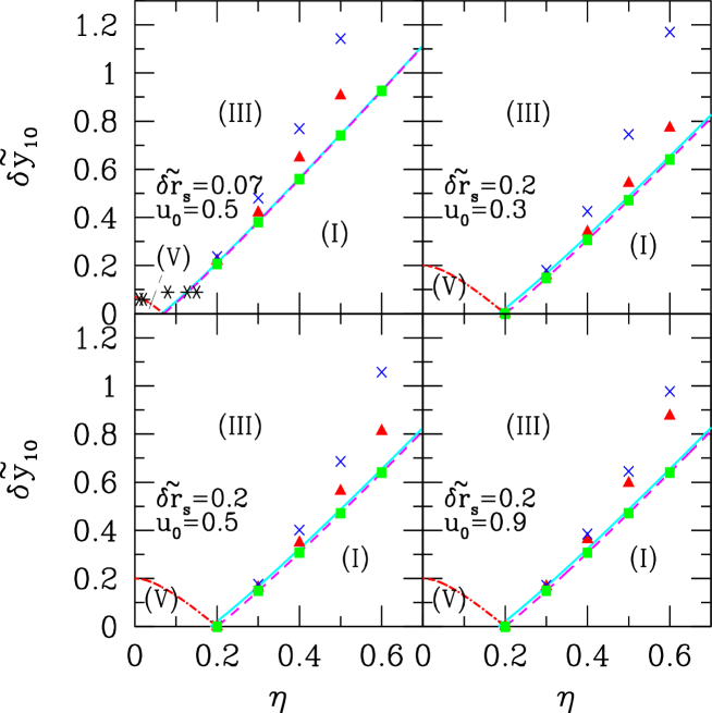
Figure 11: Boundary of the type I, III and V on the $\eta-\widetilde{\delta y_{10}}$ plane. The dashed curves satisfy $\widetilde{\Delta}^{2}_{+}=0$, the dot-dashed curves satisfy $\widetilde{\Delta}^{2}_{-}=0$, which are obtained by solving Eq. (68) of the sign $+$ and $-$, respectively, while the solid curves plot Eq. (71). In order to show the validity of the approximate approach, we plot the points of the critical configuration type II, the crosses are the exact approach (a), the triangles are the perturbative approach (b), and the squares are the approximate approach(c), respectively. The five asterisks in the upper left panel correspond to the value of $\eta$ and $\widetilde{\delta y_{10}}$ of Figs. 1 $\sim$ 5 from the right to left, respectively.

4.2 Relation with caustics and critical line

We consider the condition that the circumference of the source comes in contact with the caustics. The intersection point is obtained by substituting Eqs. (59) and (60) into Eqs. (24) and (25), which yields

$$\left({\partial^{2}\widetilde{\delta\phi}\over\partial\theta^{2}}\Bigr{|}_{x=1}\right)^{2}+\left({\partial\widetilde{\delta\phi}\over\partial\theta}\Bigr{|}_{x=1}\right)^{2}+\widetilde{\delta y_{10}}^{2}$$

$$~{}~{}~{}~{}~{}~{}~{}-2\widetilde{\delta y_{10}}\left({\partial^{2}\widetilde{\delta\phi}\over\partial\theta^{2}}\Bigr{|}_{x=1}\cos\theta+{\partial\widetilde{\delta\phi}\over\partial\theta}\Bigr{|}_{x=1}\sin\theta\right)=\widetilde{\delta r_{s}}^{2},$$ (73)

where we used $\widetilde{\delta y_{20}}=0$. Within the approximate approach (c), we use Eqs. (125) and (126), which we substitute into Eq. (73), then

$$g(\theta)\equiv 12\eta^{2}\cos^{4}\theta-4\eta\widetilde{\delta y_{10}}\cos^{3}\theta-12\eta^{2}\cos^{2}\theta+4\eta^{2}+\widetilde{\delta y_{10}}^{2}-\widetilde{\delta r_{s}}^{2}=0.$$

(74)

When the circumference of the source comes in contact with the caustics, the solution of Eq. (74) has only one solution. This condition is

$$g(\theta_{c})=0,$$ (75)

where $\theta_{c}$ satisfies

$${dg(\theta)\over d\theta}\bigg{|}_{\theta=\theta_{c}}=0.$$ (76)

The solution of Eq. (76) is

$$\theta_{c\pm}=\cos^{-1}\left[{1\over 8\eta}\left(\widetilde{\delta y_{10}}\pm\sqrt{32\eta^{2}+\widetilde{\delta y_{10}}^{2}}\right)\right],$$ (77)

then, Eq.(75) gives

$$g(\theta_{c\pm})= \frac{1}{128\eta^{2}}\Bigl{[}-\delta y_{10}^{4}+80\eta^{2}\delta y_{10}^{2}+128\eta^{4}\pm\delta y_{10}^{3}\sqrt{32\eta^{2}+\delta y_{10}^{2}}$$ (78)

$$~{}~{}\pm 32\eta^{2}\delta y_{10}\sqrt{32\eta^{2}+\delta y_{10}^{2}}+128\eta^{2}\delta r_{s}^{2}\Bigr{]}=0.$$

This is the condition that the circumference of the source comes in contact with the caustics. Note that $\theta_{c\pm}=\theta_{min\pm}$, and $g(\theta_{c\pm})=\widetilde{\Delta}_{\pm}^{2}$. This means that the critical configuration type II (plus sign) and type IV (minus sign) appear when the circumference of the source comes in contact with the caustics.

This condition can be transformed to the following relation between the critical line and the image. From Eq. (52), the central line of the image can be defined by

$$\widetilde{\delta x}={1\over(1-\partial_{\tilde{x}}^{2}\widetilde{\phi_{0}}(\widetilde{x}))}\Bigl{[}\partial_{\widetilde{x}}\widetilde{\delta\phi}(\widetilde{x},\theta)+\widetilde{\delta y_{10}}\cos\theta\Bigr{]}\Bigr{|}_{\widetilde{x}=1}.$$ (79)

The critical line is defined by Eq. (58), then an intersection point of the critical line and the central line of the image satisfies

$$\widetilde{\delta y_{10}}\cos\theta={\partial^{2}\widetilde{\delta\phi}\over\partial\theta^{2}}\Bigr{|}_{x=1}.$$ (80)

Within the approximate approach (c), using Eq. (126), this condition gives

$$\widetilde{\delta y_{10}}\cos\theta=2\eta\cos 2\theta,$$ (81)

which can be solved easily,

$$\cos\theta_{\rm cri\pm}={1\over 8\eta}\left(\widetilde{\delta y_{10}}\pm\sqrt{32\eta^{2}+\widetilde{\delta y_{10}}^{2}}\right).$$ (82)

Note that $\theta_{\rm cri\pm}=\theta_{\rm min\pm}(=\theta_{c\pm})$.

The above behaviour of the critical configuration is obtained using the approximate approach (c), but holds in the exact approach in a similar way. Indeed, these critical behaviour can be seen in Figs. 2 and 4. These facts also guarantee the usefulness of the approximate approach to investigate the lensing phenomena in a simple analytic way.

4.3 Application of approximate approach

In this subsection, let us summarise a few useful consequences, which are obtained using the approximate approach in an analytic manner.

First, we consider the width of lensed images. Within the perturbative approach, the width of the image is

$$\widetilde{\delta x_{+}}-\widetilde{\delta x_{-}} = {2\over(1-\partial_{\tilde{x}}^{2}\phi_{0}(\widetilde{x}))}\sqrt{\Delta^{2}(\widetilde{x},\theta)}\biggr{|}_{\widetilde{x}=1}.$$ (83)

From Eq. (65), the maximum width at $\theta=\theta_{\rm max}$ is

$$(\widetilde{\delta x_{+}}-\widetilde{\delta x_{-}})_{\rm max} = {2\widetilde{\delta r_{s}}\over(1-\partial_{\tilde{x}}^{2}\phi_{0}(\widetilde{x}))}.$$ (84)

From Eq. (67), the same maximum width appears at $\theta=0$ and $\pi$.

Second, let us consider the angular size of the arc, which can be obtained by solving $\widetilde{\Delta}^{2}(\theta)=0$ under the condition $\widetilde{\Delta}^{2}_{+}>0$, because $\widetilde{\Delta}^{2}(\theta)\geq 0$ is necessary for the appearance of the image. Using Eq. (61), $\widetilde{\Delta}^{2}(\widetilde{x}=1,\theta)=0$ reduces to

$$\widetilde{\delta r_{s}}^{2}-(\eta\sin 2\theta-\widetilde{\delta y_{10}}\sin\theta)^{2}=0,$$ (85)

which can be solved easily with a suitable method.

Third, we focus on the magnification of the lensed image. The magnification factor of an extended source is written (e.g.,[12]),

$$\mu_{e}={\int\mathrm{d}^{2}yI(\vec{y})\mu(\vec{y})\over\int\mathrm{d}^{2}yI(\vec{y})},$$ (86)

where $I(\vec{y})$ is the surface brightness at $\vec{y}$. In the case the surface brightness is a constant, i.e., $I(\vec{y})=I_{0}$, we may write

$$\mu_{e}={\int_{|\widetilde{\vec{y}}|<\delta r_{s}}\mathrm{d}^{2}\widetilde{\vec{y}}\mu(\widetilde{\vec{y}})\over\pi\widetilde{\delta r_{s}}^{2}}.$$ (87)

From the definition of the magnification $\mu$, we have

$$\mu_{e}=\int d\theta{dA\over d\theta},$$ (88)

where we defined

$${dA\over d\theta}={1\over\pi\widetilde{\delta r_{s}}^{2}}\int^{1+\widetilde{\delta x_{+}}}_{1+\widetilde{\delta x_{-}}}\widetilde{r^{\prime}}\mathrm{d}\widetilde{r^{\prime}}={1\over\pi\widetilde{\delta r_{s}}^{2}}(\widetilde{\delta x_{+}}-\widetilde{\delta x_{-}}).$$ (89)

Within the perturbative approach, we have

$${dA\over d\theta} = {1\over\pi\widetilde{\delta r_{s}}^{2}}{2\sqrt{\Delta^{2}(\widetilde{x},\theta)}\over(1-\partial_{\tilde{x}}^{2}\phi_{0}(\widetilde{x}))}\biggr{|}_{\widetilde{x}=1}.$$ (90)

In the approximate method (c), we may substitute the expression (61) into Eq. (90).

Fig. 12 shows $dA/d\theta$ as a function of $\theta$. In each panel, a different set of the parameters $\widetilde{\delta r_{s}}$, $\widetilde{\delta y_{10}}$, $\eta$ and $u_{0}$ is adopted, as shown therein. The solid curves show the exact approach (a), the dashed curves show the perturbative approach (b), and the long dash-dotted curves show the approximate approach (c). The top left panel adopts the same parameters as those of Fig. 1. In the top right panel, $\widetilde{\delta r_{s}}$ is increased compared with the top left panel. This increase of $\widetilde{\delta r_{s}}$ changes the four lensed images to one arc and the other separated image. In the middle left (right) panel, compared with the top left panel, $u_{0}$ is decreased (increased), by which the amplification is increased (decreased). In the lower left panel, compared with the top left panel, $\widetilde{\delta y_{10}}$ is increased, by which the four separate images change to one arc and the other separated image. In the lower right panel, $\eta$ is increased.

From Eqs. (65) and (67), we have $\Delta^{2}(\widetilde{x}=1,\theta)=\widetilde{\delta r_{s}}^{2}$ for $\theta=0,~{}\theta_{\rm max},~{}\pi$, where the width of the image becomes maximum. Then, the maximum value of $dA/d\theta$ is

$${dA\over d\theta}={2\over\pi\widetilde{\delta r_{s}}(1-\partial_{\tilde{x}}^{2}\phi_{0}(\widetilde{x}))|_{\widetilde{x}=1}}.$$ (91)

Thus, $dA/d\theta$ takes the same value at $\theta=0,~{}\theta_{\rm max},~{}\pi$, which can be also seen from Fig. 12.

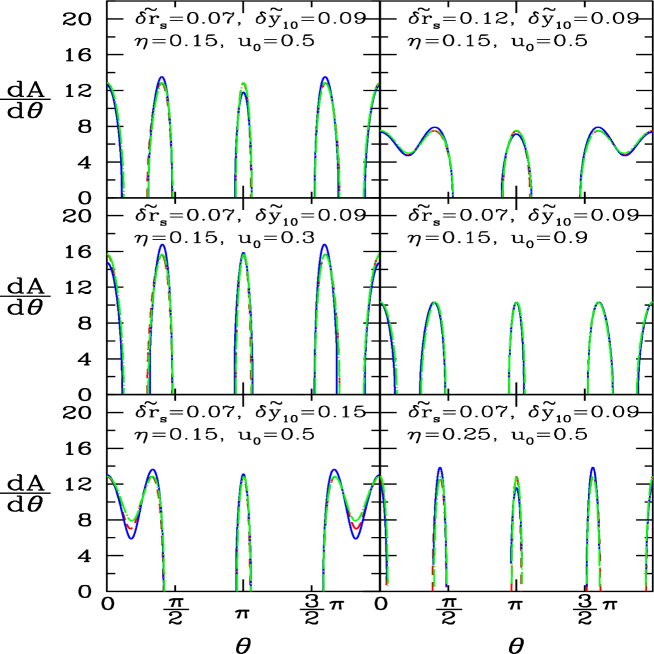
Figure 12: $dA/d\theta$ as a function of $\theta$. A different set of the parameters $\widetilde{\delta r_{s}}$, $\widetilde{\delta y_{10}}$, $\eta$ and $u_{0}$ are adopted for each panel as shown therein. The solid curves are the exact approach (a), the dashed curves are the perturbative approach (b), and the long dash-dotted curves are the approximate approach (c).

4.4 Point source limit

Finally, in this section, we consider the limit of a point source, which is given by imposing $\widetilde{\delta r_{s}}=0$. In this limit, Eq. (53) yields

$$\widetilde{\Delta}^{2}(\widetilde{x},\theta)=-\Bigl{(}{1\over\widetilde{x}}\partial_{\theta}\widetilde{\delta\phi}(\widetilde{x},\theta)-\widetilde{\delta y_{10}}\sin\theta+\widetilde{\delta y_{20}}\cos\theta\Bigr{)}^{2}.$$ (92)

For the existence of the solution, we must have $\widetilde{\Delta}(\widetilde{x},\theta)=0$. In the approximate approach (c), with the use of Eq. (125), $\widetilde{\Delta}(\widetilde{x}=1,\theta)=0$ yields

$$\eta\sin 2\theta-\widetilde{\delta}y_{10}\sin\theta+\widetilde{\delta y_{20}}\cos\theta=0.$$ (93)

This equation is equivalent to

$$\eta\sin 2\theta-\sqrt{\widetilde{\delta y_{10}}^{2}+\widetilde{\delta y_{20}}^{2}}\sin(\theta-\theta_{0})=0,$$ (94)

where $\theta_{0}=\arctan(\widetilde{\delta}y_{20}/\widetilde{\delta}y_{10})$ is regarded as an inclination angle when choosing the coordinate so that the point source is located on the $\widetilde{y_{1}}$-axis. It is easy to solve Eq. (94) in a numerical method. When a solution of Eq. (94) is found, which we denote by $\theta_{p}$, from Eqs. (52) and (56), we obtain the image position and the magnification factor,

$$\widetilde{\delta x}={1\over(1-\partial_{\tilde{x}}^{2}\widetilde{\phi_{0}}(\widetilde{x}))}\Bigl{[}\partial_{\widetilde{x}}\widetilde{\delta\phi}(\widetilde{x},\theta)+\widetilde{\delta y_{10}}\cos\theta\Bigr{]}\Biggr{|}_{\widetilde{x}=1,\theta=\theta_{p}}$$ (95)

and

$$\mu\simeq\biggl{[}(1-\partial_{\tilde{x}}^{2}\widetilde{\phi_{0}}(\widetilde{x}))\left(\widetilde{\delta y_{10}}\cos\theta-2\eta\cos 2\theta\right)\biggr{]}^{-1}\biggr{|}_{\widetilde{x}=1,\theta=\theta_{p}},$$ (96)

respectively.

For simplicity, we here consider the case $\widetilde{\delta y_{20}}=0$, that is, the inclination angle is zero. In this case, Eqs. (95) and (96) yield simple analytic expressions, as follows. Eq. (93) reduces to

$$\eta\sin 2\theta-\widetilde{\delta}y_{10}\sin\theta=0,$$ (97)

which gives the following solution to represent the angular position of the image,

$$\cos\theta_{p}=\frac{\widetilde{\delta y_{10}}}{2\eta}$$ (98)

and

$$\sin\theta_{p}=0.$$ (99)

Eq. (95) gives the radial position of the image. For the solution of Eq.(98), we have

$$\widetilde{\delta x}={1\over(1-\partial_{\tilde{x}}^{2}\widetilde{\phi_{0}}(\widetilde{x}))}\Bigl{[}\partial_{\widetilde{x}}\widetilde{\delta\phi}(\widetilde{x},\theta)+\frac{\widetilde{\delta y_{10}}^{2}}{2\eta}\Bigr{]}\Bigr{|}_{\widetilde{x}=1,\theta=\theta_{p}}.$$ (100)

By substituting Eq. (100) into Eq. (96), we have the magnification factor,

$$\mu=\biggl{[}(1-\partial_{\tilde{x}}^{2}\widetilde{\phi_{0}}(\widetilde{x}))\left(\frac{\widetilde{\delta y_{10}}^{2}}{2\eta}-{\partial^{2}\widetilde{\delta\phi}\over\partial\theta^{2}}\right)\biggr{]}^{-1}\biggr{|}_{\widetilde{x}=1,\theta=\theta_{p}}.$$ (101)

In the approximate approach (c), using Eqs. (126) and (98), this magnification factor is expressed

$$\mu\simeq\biggl{[}2\eta(1-\partial_{\tilde{x}}^{2}\widetilde{\phi_{0}}(\widetilde{x}))\left(1-\left(\frac{\widetilde{\delta y_{10}}}{2\eta}\right)^{2}\right)\biggr{]}^{-1}\biggr{|}_{\widetilde{x}=1}.$$ (102)

In the same way, for the solution of Eq. (99), we obtain the radial position of the image,

$$\widetilde{\delta x}={1\over(1-\partial_{\tilde{x}}^{2}\widetilde{\phi_{0}}(\widetilde{x}))}\biggl{[}\partial_{\widetilde{x}}\widetilde{\delta\phi}(\widetilde{x},\theta)\pm\widetilde{\delta y_{10}}\biggr{]}\Bigr{|}_{\widetilde{x}=1,\theta=\theta_{p}},$$ (103)

and the magnification factor,

$$\mu\simeq\biggl{[}2\eta(1-\partial_{\tilde{x}}^{2}\widetilde{\phi_{0}}(\widetilde{x}))\left(-1\pm\frac{\widetilde{\delta y_{10}}}{2\eta}\right)\biggr{]}^{-1}\biggr{|}_{\widetilde{x}=1},$$ (104)

where $\partial_{\tilde{x}}^{2}\widetilde{\phi_{0}}(\widetilde{x})\bigr{|}_{\widetilde{x}=1}$ is given by Eq. (119), where the sign $+$ and $-$ correspond to the solution $\theta_{p}=0$ and $\theta_{p}=\pi$, respectively, from Eq. (99).

5 Summary and Conclusions

We studied the perturbative approach to the strong lensing system, which was extended by Alard, in both the analytic and numerical manners. We investigated the validity of the perturbative approach by comparing with the exact approach on the basis of the numerical method, focusing on the shape of the image, the magnification, the caustics, and the critical line. The perturbative approach works well in the case when the ellipticity of the lens potential $\eta$ is small and the configuration of the source is close to the that of an Einstein ring. At a quantitative level, the perturbative approach is valid at the $10$ percent level for $\widetilde{\delta y_{10}}\lower 2.15277pt\hbox{$\;\buildrel<\over{\sim}\;$}0.2$ and $\eta\lower 2.15277pt\hbox{$\;\buildrel<\over{\sim}\;$}0.3$. We also demonstrated that the lowest-order expansion in terms of $\eta$ also works well, which enables us to investigate the lensing system in an analytic way.

We investigated the critical behaviour of the lensed images, by demonstrating the phase diagram of the different configurations of four separated images (type I), an arc and one separated image (type III), and one connected ring image (type V). The critical configuration of type II appears during the transition from the type I to the type III, while the type IV appears during the transition from the type III to the type V. We investigated how the critical behaviour depends on the lens ellipticity, the source position and the source radius. We also demonstrated how the appearance of the critical configuration III and V is related to the condition between the source configuration and the caustics. The condition of the critical configuration was investigated in an analytic manner using the lowest-order expansion of the ellipticity $\eta$ of the elliptical lens potential.

The perturbative approach with the lowest-order expansion with respect to $\eta$ is useful to find the simple formulas which characterises the lensing system in an analytic manner. We derived the analytical formulas of the arc width and the magnification factor. In the point source limit, the simple formulas for the image position and magnification factor were obtained. These formulas can be easily solved, which gave the simple analytic expressions in the absence from the inclination angle. These results will be useful to understand the gravitational lensing phenomena.

In a realistic situation in reconstructing a gravitational lensing system, substructures in the lens might have to be taken into account. In the reference,[16] Alard considered how a substructure affects a lensed image in the perturbative approach. Even a substructure with small mass could make a change in the caustics and the lensed image drastically. It is an interesting problem how one can determine the gravitational lens potential including substructures simultaneously. Here, there is potentially a lot of room for improvement.[17] This issue is outside the scope of the present paper, but need to be elaborated for a precise reconstruction of a gravitational lens system.

Appendix A Formulas in the exact approach

In this appendix, we summarize formulas of the lens equation in the exact approach (a) without any approximation. We consider the lensed image of the circumference of the circular source, whose center is located at $(\widetilde{\delta y_{10}},\widetilde{\delta y_{20}})$. The source’s radius is $\widetilde{\delta r_{s}}$. The circumference of the circular source is parameterized as

$$\widetilde{y_{1}}=\widetilde{\delta y_{10}}+\widetilde{\delta r_{s}}\cos\varphi,$$ (105)

$$\widetilde{y_{2}}=\widetilde{\delta y_{20}}+\widetilde{\delta r_{s}}\cos\varphi$$ (106)

with the parameter $\varphi$ in the range $0\leq\varphi\leq 2\pi$. As the image is parameterized as

$$\widetilde{x_{1}}=\widetilde{x}\cos\theta,$$ (107)

$$\widetilde{x_{2}}=\widetilde{x}\sin\theta,$$ (108)

the lens equation is

$$\widetilde{\delta y_{10}}+\widetilde{\delta r_{s}}\cos\varphi=\widetilde{x}\cos\theta-{\cos\theta}{\partial\over\partial\widetilde{x}}\widetilde{\phi}(\widetilde{x},\theta)+{\sin\theta\over\widetilde{x}}{\partial\over\partial\theta}\widetilde{\phi}(\widetilde{x},\theta),$$ (109)

$$\widetilde{\delta y_{20}}+\widetilde{\delta r_{s}}\sin\varphi=\widetilde{x}\sin\theta-{\sin\theta}{\partial\over\partial\widetilde{x}}\widetilde{\phi}(\widetilde{x},\theta)-{\cos\theta\over\widetilde{x}}{\partial\over\partial\theta}\widetilde{\phi}(\widetilde{x},\theta),$$ (110)

which yield

$$\widetilde{x}=\widetilde{\delta y_{10}}\cos\theta+\widetilde{\delta y_{20}}\sin\theta+{\partial\over\partial\widetilde{x}}\widetilde{\phi}(\widetilde{x},\theta)$$

$$~{}~{}~{}\pm\sqrt{\widetilde{\delta r_{s}}^{2}-\left({1\over\widetilde{x}}{\partial\over\partial\theta}\widetilde{\phi}(\widetilde{x},\theta)-\widetilde{\delta y_{10}}\sin\theta+\widetilde{\delta y_{20}}\cos\theta\right)^{2}},$$ (111)

and

$$\tan(\theta-\varphi)=\left[{1\over\widetilde{x}}{\partial\over\partial\theta}\widetilde{\phi}(\widetilde{x},\theta)-\widetilde{\delta y_{10}}\sin\theta+\widetilde{\delta y_{20}}\cos\theta\right]$$

$$~{}~{}~{}~{}~{}~{}~{}~{}~{}~{}~{}~{}~{}~{}~{}\times\left[\widetilde{x}-{\partial\over\partial\widetilde{x}}\widetilde{\phi}(\widetilde{x},\theta)-\widetilde{\delta y_{10}}\cos\theta-\widetilde{\delta y_{20}}\sin\theta\right]^{-1}.$$ (112)

For the elliptical NFW lens model adopted in this paper, the potential is written,

$$\widetilde{\phi}={4\kappa_{s}\over u_{0}^{2}}{1\over\widetilde{x}}\biggl{(}\log{\Xi\over 2}-2{\rm arctanh}^{2}\sqrt{{1-\Xi}\over 1+\Xi}\biggr{)},$$ (113)

where we defined $\Xi=u_{0}\widetilde{x}\sqrt{1-\eta\cos 2\theta}$. Here, the expression of the case $\Xi<1$ is presented. Eq. (113) gives

$${\partial\widetilde{\phi}\over\partial\tilde{x}}={4\kappa_{s}\over u_{0}^{2}}{1\over\widetilde{x}}\biggl{(}\log{\Xi\over 2}+{2\over\sqrt{1-\Xi^{2}}}{\rm arctanh}\sqrt{1-\Xi\over 1+\Xi}\biggr{)},$$ (114)

$${\partial\widetilde{\phi}\over\partial\theta}={4\kappa_{s}\over u_{0}^{2}}{\eta\sin 2\theta\over(1-\eta\cos 2\theta)}\biggl{(}\log{\Xi\over 2}+{2\over\sqrt{1-\Xi^{2}}}{\rm arctanh}\sqrt{1-\Xi\over 1+\Xi}\biggr{)},$$ (115)

$${\partial\widetilde{\phi}\over\partial\theta\partial\tilde{x}}={4\kappa_{s}\over u_{0}^{2}}u_{0}^{2}\eta\tilde{x}\sin 2\theta\biggl{(}{1\over\Xi^{2}-1}$$

$$~{}~{}~{}~{}~{}~{}+{1\over(1-\Xi^{2})^{3/2}}{\rm arctanh}\sqrt{1-\Xi\over 1+\Xi}\biggr{)},$$ (116)

$${\partial\widetilde{\phi}\over\partial\tilde{x}^{2}}={4\kappa_{s}\over u_{0}^{2}}{1\over\widetilde{x}^{2}}\biggl{(}-\log{\Xi\over 2}-{\Xi^{2}\over 1-\Xi^{2}}$$

$$~{}~{}~{}~{}~{}~{}+{2(-1+2\Xi^{2})\over\sqrt{1-\Xi^{2}}}{\rm arctanh}\sqrt{1-\Xi\over 1+\Xi}\biggr{)},$$ (117)

$${\partial\widetilde{\phi}\over\partial\tilde{\theta}^{2}}={4\kappa_{s}\over u_{0}^{2}}\biggl{(}{2\eta(\cos 2\theta-\eta)\over(1-\eta\cos 2\theta)^{2}}\log{\Xi\over 2}-{u_{0}^{2}\widetilde{x}^{2}\eta^{2}\sin^{2}2\theta\over(1-\eta\cos 2\theta)(1-\Xi^{2})}$$

$$~{}~{}~{}~{}~{}~{}{4\eta(1-\Xi^{2})(\cos 2\theta-\eta)+2\eta^{2}\Xi^{2}\sin^{2}2\theta\over(1-\eta\cos 2\theta)^{2}(1-\Xi^{2})^{3/2}}{\rm arctanh}\sqrt{1-\Xi\over 1+\Xi}\biggr{)}.$$ (118)

The case $\Xi<1$ is given by the analytic continuation.

Appendix B Formulas in the perturbative approach

We here summarise useful formulas in the perturbative approach (b). For the elliptical NFW lens potential, we have

$${\partial^{2}\over\partial{\widetilde{x}}^{2}}\widetilde{\phi}_{0}\Bigr{|}_{\widetilde{x}=1}={4\kappa_{s}\over u_{0}^{2}}\biggl{(}-\log{u_{0}\over 2}-{u_{0}^{2}\over 1-u_{0}^{2}}$$

$$~{}~{}~{}~{}~{}~{}+2{-1+2u_{0}^{2}\over(1-u_{0}^{2})^{3/2}}{\rm arctanh}\sqrt{1-u_{0}\over 1+u_{0}}\biggr{)},$$ (119)

$${\partial\over\partial{\widetilde{x}}}\widetilde{\delta\phi}\Bigr{|}_{\widetilde{x}=1}={4\kappa_{s}\over u_{0}^{2}}\biggl{(}\log\Upsilon-{2\over\sqrt{1-u_{0}^{2}}}{\rm arctanh}\sqrt{1-u_{0}\over 1+u_{0}}$$

$$~{}~{}~{}~{}~{}~{}~{}~{}~{}+{2\over\sqrt{1-u_{0}^{2}\Upsilon^{2}}}{\rm arctanh}\sqrt{{1-u_{0}\Upsilon}\over 1+u_{0}\Upsilon}\biggr{)},$$ (120)

$${\partial\over\partial{\theta}}\widetilde{\delta\phi}\Bigr{|}_{\widetilde{x}=1}={4\kappa_{s}\over u_{0}^{2}}{\eta\sin 2\theta\over\Upsilon^{2}}\biggl{(}\log{u_{0}\Upsilon\over 2}$$

$$~{}~{}~{}~{}~{}~{}~{}~{}~{}+{2\over\sqrt{1-u_{0}^{2}\Upsilon^{2}}}{\rm arctanh}\sqrt{{1-u_{0}\Upsilon}\over 1+u_{0}\Upsilon}\biggr{)},$$ (121)

$${\partial^{2}\over\partial{\theta}^{2}}\widetilde{\delta\phi}\Bigr{|}_{\widetilde{x}=1}={4\kappa_{s}\over u_{0}^{2}}{1\over\Upsilon^{4}}\biggl{(}2(1-\Upsilon^{2}-\eta^{2})\log{u_{0}\Upsilon\over 2}$$

$$~{}~{}~{}~{}~{}~{}~{}~{}~{}+{2\eta^{2}u_{0}^{2}\Upsilon^{2}\sin 2\theta\over\sqrt{1-u_{0}^{2}\Upsilon^{2}}^{3}}{\rm arctanh}\sqrt{{1-u_{0}\Upsilon}\over 1+u_{0}\Upsilon}$$

$$~{}~{}~{}~{}~{}~{}~{}~{}~{}+{4(1-\Upsilon^{2}-\eta^{2})\over\sqrt{1-u_{0}^{2}\Upsilon^{2}}}{\rm arctanh}\sqrt{{1-u_{0}\Upsilon}\over 1+u_{0}\Upsilon}\biggr{)}$$

$$~{}~{}~{}~{}~{}~{}~{}~{}~{}-{\eta^{2}u_{0}^{2}\Upsilon^{2}\sin^{2}2\theta\over 1-u_{0}^{2}\Upsilon^{2}}\biggr{)},$$ (122)

where we defined $\Upsilon=\sqrt{1-\eta\cos 2\theta}$.

Appendix C Formulas in the approximate approach

In the approximate approach (c), the potential is approximated at the lowest order of expansion with respect to $\eta$. The following formulas are useful. By expanding the potential $\widetilde{\delta\phi}$, Eq. (51), we have

$$\widetilde{\delta\phi}(\widetilde{x},\theta)\simeq{4\kappa_{s}\over u_{0}^{2}}\eta\cos 2\theta\biggl{(}-{1\over 2}\log{u_{0}\widetilde{x}\over 2}-{1\over(1-u_{0}^{2})^{1/2}}{\rm arctanh}\sqrt{1-u_{0}\widetilde{x}\over 1+u_{0}\widetilde{x}}\biggr{)},$$

(123)

at the lowest order of $\eta$. Similarly, Eqs. (120)$\sim$(122) lead to

$${\partial\over\partial{\widetilde{x}}}\widetilde{\delta\phi}\Bigr{|}_{\widetilde{x}=1}\simeq{4\kappa_{s}\over u_{0}^{2}}\eta\cos 2\theta\biggl{(}{u_{0}^{2}\over 2(1-u_{0}^{2})}-{u_{0}^{2}\over(1-u_{0}^{2})^{3/2}}{\rm arctanh}\sqrt{1-u_{0}\over 1+u_{0}}\biggr{)},$$

(124)

$${\partial\over\partial{\theta}}\widetilde{\delta\phi}\Bigr{|}_{\widetilde{x}=1}\simeq{\eta\sin 2\theta},$$ (125)

$${\partial^{2}\over\partial{\theta}^{2}}\widetilde{\delta\phi}\Bigr{|}_{\widetilde{x}=1}\simeq{2\eta\cos 2\theta}.$$ (126)

References

- [1] E. Komatsu et al., arXiv:1001.4538.
- [2] E. Zackrisson and T. Riehm, Advances in Astronomy, 2010 (2010) 1.
- [3] C. S. Kochanek, C. R. Keeton and B. A. McLeod, Astrophys. J. 547 (2001) 50.
- [4] T. Futamase and T. Hamana, Prog. Theor. Phys. 102 (1999) 1037.
- [5] T. Futamase and S. Yoshida, Prog. Theor. Phys. 105 (2001) 887.
- [6] K. Yamamoto and T. Futamase, Prog. Theor. Phys. 105 (2001) 707.
- [7] K. Yamamoto, Y. Kadoya, T. Murata and T. Futamase, Prog. Theor. Phys. 106 (2001) 917.
- [8] T. Futamase, Int. J. Mod. Phys. A17 (2002) 2677.
- [9] M. Oguri et al., Astron. J. 135 (2008) 512.
- [10] P. A. Abel et al., arXiv:0912.0201 .
- [11] R. D. Blandford and I. Kovner, Phys. Rev. A38 (1988) 4028.
- [12] P. Schneider, J. Ehlers and E. E. Falco, Gravitational Lenses, (Springer-Verlag, New York, 1992).
- [13] J. F. Navarro, C. S. Frenk and S. D. M. White, Astrophys. J. 462 (1996) 563.
- [14] J. F. Navarro, C. S. Frenk and S. D. M. White, Astrophys. J. 490 (1997) 493.
- [15] C. Alard, Mon. Not. R. Astron. Soc. 382 (2007) L58.
- [16] C. Alard, Mon. Not. R. Astron. Soc. 388 (2008) 375.
- [17] C. Alard, Astron. & Astrophys. 506 (2009) 609.
- [18] C. Alard, Astron. & Astrophys. 513 (2010) 39.
- [19] S. Peirani, C. Alard, C. Pichon, R. Gavazzi and D. Aubert, Mon. Not. R. Astron. Soc. 390 (2008) 945.
- [20] M. Bartelmann, Astron. & Astrophys. 313 (1996) 697-702.