Optimal interpolation formulas in the periodic function space of S.L. Sobolev

Abstract.

In this paper the problem of construction of lattice optimal interpolation formulas in the space $\widetilde{L_{2}^{(m)}}(0,1)$ is considered. Using S.L. Sobolev’s method explicit formulas for the coefficients of lattice optimal interpolation formulas are given and the norm of the error functional of lattice optimal interpolation formulas is calculated. Moreover, connection between optimal interpolation formula in the space $\widetilde{L_{2}^{(m)}}(0,1)$ and optimal quadrature formula in this space is shown. Finally, numerical results are given.

MSC: 41A05, 41A15, 65D30, 65D32.

Keywords: lattice optimal interpolation formula; error functional; optimal coefficients; S.L. Sobolev space; periodic function.

1. Introduction. Statement of the Problem

In order to find an approximate representation of a function $\varphi(x)$ by elements of a certain finite dimensional space, it is possible to use values of this function at some finite set of points $x_{k}$, $k=1,2,...,N$. The corresponding problem is called the interpolation problem, and the points $x_{k}$ the interpolation nodes.

There are polynomial and spline interpolations. Now the theory of spline interpolation is fast developing. Many books are devoted to the theory of splines, for example, Ahlberg et al [1], de Boor [2], Schumaker [3], Laurent [4], Attea [5], Stechkin and Subbotin [6], Vasilenko [7], Arcangeli et al [8], Ignatov and Pevniy [9], Korneichuk et al [10], in the numerical analysis literature or Wahba [11], Eubank [12], Green and Silverman [13], Berlinet and Thomas-Agnan [14] in the statistical one.

If the exact values $\varphi(x_{k})$ of an unknown smooth function $\varphi(x)$ at the set of points $\{x_{k},\ k=1,2,...,N\}$ in an interval $[a,b]$ are known, it is usual to approximate $\varphi$ by minimizing

(1.1) $$\int_{a}^{b}(g^{(m)}(x))^{2}dx$$

in the set of interpolating functions (i.e. $g(x_{k})=\varphi(x_{k})$, $k=1,2,...,N$) of the Sobolev space $L_{2}^{(m)}(a,b)$. It turns out that the solution is a natural polynomial spline of order $2m$ with knots $x_{1},...,x_{N}$ called the interpolating $D^{m}$ spline for the points $(x_{k},\varphi(x_{k}))$. In non periodic case first this problem was investigated by Holladay [15] for $m=2$ and the result of Holladay was generalized by de Boor [16] for any $m$. In the Sobolev space $\widetilde{L_{2}^{(m)}}$ of periodic functions the minimization problem of integrals of type (1.1) were investigated by I.J.Schoenberg [17] and M.Golomb [18].

In the present paper we deal with optimal interpolation formulas. Now we give the statement of the problem of optimal interpolation formulas following by S.L.Sobolev [19]. It should be noted that connection between the minimization problem of integrals of type (1.1) and the problem of optimal formulas was shown in [20].

First we recall the definition of Sobolev space $\widetilde{L_{2}^{(m)}}(0,1)$ of periodic functions (see [21, 22]).

Suppose in the set $\mathbb{R}$ of real numbers the function $\varphi(x)$ has local summable derivatives up to order $m$, and also for the interval $[0,1]$ the integral $\int_{0}^{1}{\left({\varphi^{(m)}(x)}\right)^{2}dx}$ is bounded. Assume that the function $\varphi(x)$ is periodic: $\varphi(x+\gamma)=\varphi(x)$, $x\in\mathbb{R},\,\,\,\gamma\in\mathbb{Z}$, where $\mathbb{Z}$ is the set of integer numbers.

Every element of the space $\widetilde{L_{2}^{(m)}}(0,1)$ is a class of functions which differ from each other by constant term. The norm of functions in the space $\widetilde{L_{2}^{(m)}}(0,1)$ is defined by formula

$$\left\|{\left.{\varphi}\right|\widetilde{L_{2}^{(m)}}(0,1)}\right\|=\left({\int\limits_{0}^{1}{\left({\varphi^{(m)}(x)}\right)^{2}dx}}\right)^{1/2}.$$

Now following [19] we consider interpolation formula of the form

(1.2) $$\varphi(x)\cong P_{\varphi}(x)=\sum\limits_{k=1}^{N}{C_{k}(x)\cdot\varphi(x_{k})}$$

in the space $\widetilde{L_{2}^{(m)}}(0,1)$. Here points $x_{k}\in[0,1]$ and parameters $C_{k}(x)$ are respectively called the nodes and the coefficients of the interpolation formula (1.2).

The difference $\varphi-P_{\varphi}$ is called the error of the interpolation formula (1.2). The value of this error at some point $z$ is the linear functional on functions $\varphi$, i.e.

$$(\ell,\varphi)\equiv\varphi(z)-P_{\varphi}(z)=\varphi(z)-\sum\limits_{k=1}^{N}C_{k}(z)\varphi(x_{k})=$$

(1.3) $$=\int\limits_{0}^{1}\left[\left(\delta(x-z)-\sum\limits_{k=1}^{N}C_{k}(z)\delta(x-x_{k})\right)*\phi_{0}(x)\right]\varphi(x)dx,$$

where $\delta(x)$ is the Dirac delta-function, $\phi_{0}(x)=\sum\limits_{\beta}\delta(x-\beta)$, here $\beta$ takes all integer values and

(1.4) $$\ell=\left(\delta(x-z)-\sum\limits_{k=1}^{N}C_{k}(z)\delta(x-x_{k})\right)*\phi_{0}(x)$$

is the error functional of interpolation formula (1.2) and belongs to the space $\widetilde{L_{2}^{(m)*}}(0,1)$. The space $\widetilde{L_{2}^{(m)*}}(0,1)$ is the conjugate space to the space $\widetilde{L_{2}^{(m)}}(0,1)$ and consists of all periodic functionals (1.4) which are orthogonal to unity, i.e.

(1.5) $$(\ell,1)=0.$$

By Cauchy-Schwartz inequality

$$|(\ell,\varphi)|\leq\|\varphi|\widetilde{L_{2}^{(m)}}(0,1)\|\cdot\|\ell|\widetilde{L_{2}^{(m)*}}(0,1)\|$$

the error (1.3) of formula (1.2) is estimated with the help of the norm

$$\left\|{\ell|\widetilde{L_{2}^{(m)*}}(0,1)}\right\|=\mathop{\sup}\limits_{\left\|{\varphi|\widetilde{L_{2}^{(m)}}(0,1)}\right\|=1}\left|{\left({\ell,\varphi}\right)}\right|$$

of the error functional (1.4). Consequently, estimation of the error of interpolation formula (1.2) on functions of the space $\widetilde{L_{2}^{(m)}}(0,1)$ is reduced to finding the norm of the error functional $\ell$ in the conjugate space $\widetilde{L_{2}^{(m)*}}(0,1)$.

Therefore from here we get the first problem.

Problem 1.

Find the norm of the error functional $\ell$ of interpolation formula (1.2) in the space $\widetilde{L_{2}^{(m)*}}(0,1)$.

Obviously the norm of the error functional $\ell(x)$ depends on the coefficients $C_{k}(z)$ and the nodes $x_{k}$. By optimal interpolation formula we call such formula which the error functional in given number $N$ of the nodes has the minimum norm in the space $\widetilde{L_{2}^{(m)*}}(0,1)$. If the nodes $x_{k}$ are the points of a lattice, i.e. are located at points of the form $x_{k}=hk$ then such interpolation formula is called the lattice interpolation formula. Here $h$ is small parameter and is called the step of the lattice.

The main goal of the present paper is to construct the lattice optimal interpolation formula in the space $\widetilde{L_{2}^{(m)}}(0,1)$ for the nodes $x_{k}=hk$, i.e., to find the coefficients $C_{k}(z)$ satisfying the following equality

(1.6) $$\left\|{\mathop{\ell}\limits^{\circ}(x)|\widetilde{L_{2}^{(m)*}}(0,1)}\right\|=\mathop{\inf}\limits_{C_{k}(z)}\left\|{\mathop{\ell}\limits(x)|\widetilde{L_{2}^{(m)*}}(0,1)}\right\|.$$

Thus in order to construct the lattice optimal interpolation formula in the space $\widetilde{L_{2}^{(m)}}(0,1)$ we need to solve the next problem.

Problem 2.

Find the coefficients $C_{k}(z)$ which satisfy equality (1.6) when the nodes are located in the lattice, i.e., $x_{k}=hk$.

In the present paper the lattice optimal interpolation formulas are constructed in the Sobolev space $\widetilde{L_{2}^{(m)}}(0,1)$ of periodic functions. First such problem was stated and investigated by S.L. Sobolev in [19], where the extremal function of the interpolation formula was found in the space $W_{2}^{(m)}$.

This paper is organized as follows. In Section 2 we determine the extremal function which corresponds to the error functional $\ell(x)$ and give a representation of the norm of the error functional (1.4). Section 3 is devoted to minimization of $\left\|\ell\right\|^{2}$ with respect to the coefficients $C_{k}(z)$. We obtain a system of linear equations for the coefficients of the optimal interpolation formula in the space $\widetilde{L_{2}^{(m)}}(0,1)$. Moreover, the existence and uniqueness of the corresponding solution is proved. In Section 4 we consider the problem of construction of lattice optimal interpolation formulas. In Section 5 we prove some new properties of the discrete analogue of the differential operator $d^{2m}/dx^{2m}$. Using these properties explicit formulas for coefficients of lattice optimal interpolation formulas are found in Section 6. In Section 7 the norm of the error functional of lattice optimal interpolation formulas is calculated. Integrating obtained lattice optimal interpolation formula the optimal quadrature formula in the space $\widetilde{L_{2}^{(m)}}(0,1)$ is obtained in Section 8. Finally, in Section 9 we give formulas for coefficients which are very useful in practice and we present some numerical results.

2. The extremal function and representation
of the norm of the error functional

In this section we solve Problem 1, i.e. we find explicit form of the norm of $\ell(x)$.

For finding the explicit form of the norm of the error functional $\ell(x)$ in the space $\widetilde{L_{2}^{(m)}}(0,1)$ we use concept of its extremal function which was introduced by S.L.Sobolev [19, 21]. The function $u(x)$ from $\widetilde{L_{2}^{(m)}}(0,1)$ is called the extremal function for the error functional $\ell(x)$ if the following equality is fulfilled

$$\left({\ell,u}\right)=\left\|{\ell\left|{\widetilde{L_{2}^{(m)*}}(0,1)}\right.}\right\|\cdot\left\|{u\left|{\widetilde{L_{2}^{(m)}}(0,1)}\right.}\right\|.$$

The space $\widetilde{L_{2}^{(m)}}(0,1)$ is Hilbert space and the inner product in this space is given by formula

$$\langle{\varphi,\psi}\rangle_{m}=\int\limits_{0}^{1}{\varphi^{(m)}(x)\cdot\psi^{(m)}(x)dx}.$$

According to the Riesz theorem any linear continuous functional $\ell(x)$ in a Hilbert space is represented in the form of a inner product

(2.1) $$\left({\ell,\varphi}\right)=\langle{\psi_{\ell},\varphi}\rangle_{m}$$

for arbitrary function $\varphi(x)$ from $\widetilde{L_{2}^{(m)}}(0,1)$. Here $\psi_{\ell}(x)$ is a function from $\widetilde{L_{2}^{(m)}}(0,1)$ is defined uniquely by functional $\ell(x)$ and is the extremal function. Integrating by parts the expression in the right hand side of (2.1) and using periodicity of functions $\varphi(x)$ and $\psi_{\ell}(x)$ we get the following equality

$$\left({\ell,\varphi}\right)=(-1)^{m}\int\limits_{0}^{1}{{{d^{2m}}\over{dx^{2m}}}\psi_{\ell}(x)\cdot\varphi(x)dx}.$$

Thus the function $\psi_{\ell}(x)$ is the generalized solution of the equation

(2.2) $${{d^{2m}}\over{dx^{2m}}}\psi_{\ell}(x)=(-1)^{m}\ell(x)$$

with the boundary conditions

$$\psi_{\ell}^{(\alpha)}(0)=\psi_{\ell}^{(\alpha)}(1),\,\,\,\alpha=\overline{0,2m-1}.$$

For the extremal function the following holds

Theorem 2.1.

Explicit expression for the extremal function $\psi_{\ell}(x)$ of the error functional (1.4) is defined by formula

(2.3) $$\psi_{\ell}(x)=(-1)^{m}\left[{B_{2m}(x-z)-\sum\limits_{k=1}^{N}{C_{k}(z)\cdot B_{2m}(x-x_{k})+d_{0}}}\right],$$

where $B_{2m}(x)=\sum\limits_{\beta\neq 0}{{{\exp(-2\pi i\beta x)}\over{(2\pi i\beta)^{2m}}}}$ is the Bernoulli polynomial, $d_{0}$ is a constant.

Proof.

Here we use the following formulas of Fourier transformations given in [21]

$$F[\varphi(x)]=\int_{-\infty}^{\infty}{\exp(2\pi ipx)\cdot\varphi(x)dx},\ \ F^{-1}[\varphi(p)]=\int_{-\infty}^{\infty}{\exp(-2\pi ixp)\cdot\varphi(p)dp}.$$

Convolution of two functions is defined by formula

$$f(x)*g(x)=\int\limits_{-\infty}^{\infty}{f(x-y)\cdot g(y)dy}.$$

Applying to both sides of equation (2.2) the Fourier transformation and known formulas$F[\delta(x-z)]=e^{2\pi ipz}$, $F[\phi_{0}(x)]=\phi_{0}(p)$ (see [21]) we get

(2.4) $$(2\pi ip)^{2m}F[\psi_{\ell}(x)]=(-1)^{m}\left[{\left({\exp(2\pi ipz)-\sum\limits_{k=1}^{N}{C_{k}(z)\exp(2\pi ipx_{k})}}\right)\phi_{0}(p)}\right].$$

By virtue of (1.5) the right hand side of (2.4) is zero at the origin. Therefore we can divide both sides of (2.4) by $(2\pi ip)^{2m}$. The function $F[\psi_{\ell}(x)]$ is defined from equation (2.4) up to the following expression

$$(-1)^{m}d_{0}\delta(p)+\sum\limits_{\alpha=1}^{2m-1}{d_{\alpha}D^{\alpha}\delta(p)}.$$

But as known a periodic solution of the homogenous equation corresponding to equation (2.2) is a constant term then all terms except $(-1)^{m}d_{0}\delta(p)$ should be omitted. Thus from (2.4) we get

(2.5) $$F[\psi_{\ell}(x)]=(-1)^{m}d_{0}\delta(p)+{{\exp(2\pi ipz)\ \phi_{0}(p)}\over{(2\pi p)^{2m}}}-{{\sum\limits_{k=1}^{N}{C_{k}(z)\exp(2\pi ipx_{k})\ \phi_{0}(p)}}\over{(2\pi p)^{2m}}}.$$

Changing the function $\phi_{0}(p)$ by series of $\delta$ functions and applying the inverse Fourier transformation to both sides of (2.5) we get (2.3). Theorem 2.1 is proved. ∎

Now we obtain representation for the norm of the error functional $\ell$. Since the space $\widetilde{L_{2}^{(m)}}(0,1)$ is the Hilbert space then by the Riesz theorem we have

(2.6) $$\left({\ell,\psi_{\ell}}\right)=\left\|{\ell\left|{\widetilde{L_{2}^{(m)*}}(0,1)}\right.}\right\|\cdot\left\|{\psi_{\ell}\left|{\widetilde{L_{2}^{(m)}}(0,1)}\right.}\right\|=\left\|{\ell\left|{\left|{\widetilde{L_{2}^{(m)*}}(0,1)}\right.}\right.}\right\|^{2}.$$

Using formulas (1.4), (2.3), (2.6) we get

$$\left\|{\ell(x)\left|{\widetilde{L_{2}^{(m)*}}(0,1)}\right.}\right\|^{2} = \int\limits_{0}^{1}{\ell(x)\psi_{\ell}(x)dx=}(-1)^{m}\int\limits_{0}^{1}{\left({\delta(x-z)-\sum\limits_{k=1}^{N}{C_{k}(z)\cdot\delta(x-x_{k})}}\right)*\phi_{0}(x)}$$

$$\times\left({B_{2m}(x-z)-\sum\limits_{k=1}^{N}{C_{k}(z)\cdot B_{2m}(x-x_{k})+d_{0}}}\right)$$

$$= (-1)^{m}\int\limits_{0}^{1}{\left({\delta(x-z)*\phi_{0}(x)-\sum\limits_{k=1}^{N}{C_{k}(z)\delta(x-x_{k})*\phi_{0}(x)}}\right)}$$

$$\times\left({B_{2m}(x-z)-\sum\limits_{k=1}^{N}{C_{k}(z)\cdot B_{2m}(x-x_{k})}}\right)dx+(-1)^{m}d_{0}\left({\ell(x),1}\right).$$

Hence, using the condition (1.5) we have

$$\left\|{\ell(x)\left|{\widetilde{L_{2}^{(m)*}}(0,1)}\right.}\right\|^{2}=(-1)^{m}\int\limits_{0}^{1}{\left[{\sum\limits_{\beta}{\int\limits_{-\infty}^{\infty}{\delta(x-z-y)\delta(y-\beta)dy}-}}\right.}$$

$$\left.{-\sum\limits_{k=1}^{N}{C_{k}(z)\sum\limits_{\beta}{\int\limits_{-\infty}^{\infty}{\delta(x-x_{k}-y)\delta(y-\beta)dy}}}}\right]\left[{B_{2m}(x-z)-\sum\limits_{k=1}^{N}{C_{k}(z)\cdot B_{2m}(x-x_{k})}}\right]dx.$$

Taking into account definition of Dirac’s delta-function we obtain

$$\left\|{\ell(x)\left|{\widetilde{L_{2}^{(m)*}}(0,1)}\right.}\right\|^{2}=(-1)^{m}\int\limits_{0}^{1}{\left[{\sum\limits_{\beta}{\delta(x-z-\beta)}-\sum\limits_{k=1}^{N}{C_{k}(z)\delta(x-x_{k}-\beta)}}\right]\times}$$

$$\times\left({B_{2m}(x-z)-\sum\limits_{k=1}^{N}{C_{k}(z)\cdot B_{2m}(x-x_{k})}}\right)dx=$$

$$=(-1)^{m}\left[{\int\limits_{0}^{1}{\sum\limits_{\beta}{\delta(x-z-\beta)\cdot B_{2m}(x-z)dx}-}}\right.\sum\limits_{k=1}^{N}{C_{k}(z)\int\limits_{0}^{1}{\sum\limits_{\beta}{\delta(x-z-\beta)\cdot B_{2m}(x-x_{k})dx}}-}$$

$$-\sum\limits_{k=1}^{N}{C_{k}(z)\int\limits_{0}^{1}{\sum\limits_{\beta}{\delta(x-x_{k}-\beta)\cdot B_{2m}(x-z)dx}}+}$$

$$+\left.{\sum\limits_{k=1}^{N}{\sum\limits_{k^{\prime}=1}^{N}{C_{k}(z)C_{k^{\prime}}(z)}\sum\limits_{\beta}{\int\limits_{0}^{1}{\delta(x-x_{k}-\beta)B_{2m}(x-x_{k^{\prime}})dx}}}}\right].$$

Hence with the help of the characteristic function $\chi_{\left[{0,1}\right]}(x)$ of the interval $[0,1]$ square of the norm of the error functional (1.4) we reduce to the form

$$\left\|{\ell(x)\left|{\widetilde{L_{2}^{(m)*}}(0,1)}\right.}\right\|^{2} = (-1)^{m}\left[{\sum\limits_{\beta}{\int\limits_{-\infty}^{\infty}{\chi_{\left[{0,1}\right]}(x)\delta(x-z-\beta)\,B_{2m}(x-z)dx}}}\right.$$

$$-\sum\limits_{k=1}^{N}{C_{k}(z)\sum\limits_{\beta}{\int\limits_{-\infty}^{\infty}{\chi_{[0,1]}(x)\delta(x-z-\beta)\,B_{2m}(x-x_{k})dx}}}$$

$$-\sum\limits_{k=1}^{N}{C_{k}(z)\sum\limits_{\beta}{\int\limits_{-\infty}^{\infty}{\chi_{[0,1]}(x)\delta(x-x_{k}-\beta)\,B_{2m}(x-z)dx}}}$$

$$+\left.{\sum\limits_{k=1}^{N}{\sum\limits_{k^{\prime}=1}^{N}{C_{k}(z)C_{k^{\prime}}(z)\sum\limits_{\beta}{\int\limits_{-\infty}^{\infty}{\chi_{[0,1]}(x)\delta(x-x_{k}-\beta)\,B_{2m}(x-x_{k})dx}}}}}\right].$$

From here applying definition of Dirac’s delta-function we have

$$\left\|{\ell(x)\left|{\widetilde{L_{2}^{(m)*}}(0,1)}\right.}\right\|^{2} = (-1)^{m}\left[{\sum\limits_{\beta}{\chi_{[0,1]}(z+\beta)B_{2m}(\beta)}}\right.$$

$$-\sum\limits_{k=1}^{N}{C_{k}(z)}\sum\limits_{\beta}{\chi_{[0,1]}(z+\beta)}B_{2m}(z+\beta-x_{k})$$

$$-\sum\limits_{k=1}^{N}{C_{k}(z)}\sum\limits_{\beta}{\chi_{[0,1]}(x_{k}+\beta)}B_{2m}(x_{k}+\beta-z)$$

$$+\left.{\sum\limits_{k=1}^{N}{C_{k}(z)}\sum\limits_{k^{\prime}=1}^{N}{C_{k^{\prime}}(z)}\sum\limits_{\beta}{\chi_{[0,1]}(x_{k}+\beta)}B_{2m}(x_{k}+\beta-x_{k^{\prime}})}\right].$$

Taking into account that $x_{k}\in[0,1],\,$ $\,z\in[0,1],\,$ $\,\sum_{\beta}{\chi_{[0,1]}(y+\beta)=1}$ (see. [21]), $y\in[0,1]$, and 1-periodicity, symmetry of $B_{2m}(x)$, that is $B_{2m}(x+\gamma)=B_{2m}(x),\,\,\,B_{2m}(-x)=B_{2m}(x)$ from the last equality we get the following representation of $\|\ell(x)\|^{2}$

(2.7) $$\left\|{\ell(x)\left|{\widetilde{L_{2}^{(m)*}}(0,1)}\right.}\right\|^{2} = (-1)^{m}\left[{B_{2m}(0)-2\sum\limits_{k=1}^{N}{C_{k}(z)B_{2m}(z-x_{k})+}}\right.$$

$$+\left.{\sum\limits_{k=1}^{N}{C_{k}(z)\sum\limits_{k^{\prime}=1}^{N}{C_{k^{\prime}}(z)}B_{2m}(x_{k}-x_{k^{\prime}})}}\right].$$

Thus Problem 1 is solved.

Further in next sections we solve Problem 2.

3. Existence and uniqueness of optimal interpolation formula

For finding the minimum of the norm (2.7) under the condition (1.5) we use the Lagrange methods. For this we consider the function

$$\Psi(\mathbf{C}(z),\lambda)=\|\ell\|^{2}+2(-1)^{m}\lambda\ (\ell(x),1),$$

where $\mathbf{C}(z)=(C_{1}(z),C_{2}(z),...,C_{N}(z))$.

Equating the partial derivatives of $\Psi(\mathbf{C}(z),\lambda)$ by $C_{k}(z),\ (k=1,2,...,N)$ and $\lambda$ to zero we get the following system of linear equations

(3.1) $$\sum\limits_{k=1}^{N}C_{k}(z)B_{2m}(x_{k^{\prime}}-x_{k})+\lambda=B_{2m}(z-x_{k^{\prime}}),\ \ k^{\prime}=1,2,...,N,$$

(3.2) $$\sum\limits_{k=1}^{N}C_{k}(z)=1.$$

System (3.1)-(3.2) has a unique solution and this solution gives the minimum to $\|\ell(x)\|^{2}$ under the condition (3.2).

It should be noted that uniqueness of the solution of such type systems were also investigated in [7, 8, 9, 21, 22].

The uniqueness of the solution of system (3.1)–(3.2) is proved following [22, Chapter I]. For completeness we give it here.

First in (2.7) we change of variables $C_{k}(z)=\bar{C}_{k}(z)+d_{k}(z)$ then (2.7) and system (3.1)–(3.2) have the following form

(3.3) $$\|\ell\|^{2} = (-1)^{m}\left[\sum\limits_{k=1}^{N}\bar{C}_{k}(z)\right.\sum\limits_{k^{\prime}=1}^{N}\bar{C}_{k^{\prime}}(z)B_{2m}(x_{k}-x_{k^{\prime}})-2\sum\limits_{k=1}^{N}(\bar{C}_{k}(z)+d_{k}(z))B_{2m}(z-x_{k})$$

$$+\sum\limits_{k=1}^{N}\sum\limits_{k^{\prime}=1}^{N}\left.(d_{k}(z)d_{k^{\prime}}(z)+\bar{C}_{k}(z)d_{k^{\prime}}(z)+\bar{C}_{k^{\prime}}(z)d_{k}(z))B_{2m}(x_{k}-x_{k^{\prime}})+B_{2m}(0)\right],$$

(3.4) $$\sum\limits_{k=1}^{N}\bar{C}_{k}(z)B_{2m}(x_{k^{\prime}}-x_{k})+\lambda=B_{2m}(z-x_{k^{\prime}})-\sum\limits_{k=1}^{N}d_{k}(z)B_{2m}(x_{k^{\prime}}-x_{k}),$$

$$k^{\prime}=1,2,...,N,$$

(3.5) $$\sum\limits_{k=1}^{N}\bar{C}_{k}(z)=0,$$

where $d_{k}(z)$ is a partial solution of the equation (3.2).

Hence we directly get that the minimization of (2.7) under the condition (3.2) with respect to $C_{k}(z)$ is equivalent to the minimization of expression (3.3) with respect to $\overline{C}_{k}(z)$ under the condition (3.5). Therefore it is sufficient to prove that system (3.4)–(3.5) has a unique solution with respect to unknowns $\overline{\mathbf{C}}(z)=(\overline{C}_{1}(z),\overline{C}_{2}(z),...,\overline{C}_{N}(z)),$ $\lambda$ and this solution gives the conditional minimum for $\left\|\ell\right\|^{2}$.

From the theory of conditional extremum it is known the sufficient condition in which the solution of system (3.4)–(3.5) gives the conditional minimum for $\left\|\ell\right\|^{2}$ on manifold (3.5). It consists of positiveness of the following quadratic form

(3.6) $$\Phi(\overline{\mathbf{C}}(z))=\sum\limits_{k=1}^{N}\sum\limits_{k^{\prime}=1}^{N}{{{\partial^{2}\Psi(\overline{\mathbf{C}}(z),\lambda)}\over{\partial\overline{C}_{k}(z)\partial\overline{C}_{k^{\prime}}(z)}}}\overline{C}_{k}(z)\overline{C}_{k^{\prime}}(z)$$

on the set of vectors $\overline{\mathbf{C}}(z)=(\overline{C}_{1}(z),\overline{C}_{2}(z),...,\overline{C}_{N}(z))$ under the condition

(3.7) $$S\overline{\mathbf{C}}=0,$$

where $S=(1,1,...,1)$ is the $N$ component vector.

In our case this condition is fulfilled, i.e. the following holds

Lemma 3.1.

For any non zero vector $\overline{\mathbf{C}}(z)=(\overline{C}_{1}(z),\overline{C}_{2}(z),...,\overline{C}_{N}(z))\in\mathbb{R}^{N}$ lying in the subspace (3.7) the function $\Phi(\overline{\mathbf{C}}(z))$ is strictly positive.

Proof.

From definition of the function $\Psi(\overline{\mathbf{C}}(z),\lambda)$ and (3.6) it follows that

(3.8) $$\Phi(\overline{\mathbf{C}}(z))=2\sum_{k=1}^{N}\sum_{k^{\prime}=1}^{N}(-1)^{m}B_{2m}(x_{k}-x_{k^{\prime}})\overline{C}_{k}(z)\overline{C}_{k^{\prime}}(z).$$

We consider the functional

$$\ell_{\overline{\mathbf{C}}(z)}(x)=\sqrt{2}\sum_{k=1}^{N}\overline{C}_{k}(z)\delta(x-x_{k})*\phi_{0}(x).$$

By virtue of condition (3.7) the functional $\ell_{\overline{\mathbf{C}}(z)}(x)$ belongs to the space $\widetilde{L_{2}^{(m)*}}(0,1)$. Thus this functional has the extremal function $u_{\overline{\mathbf{C}}(z)}(x)\in\widetilde{L_{2}^{(m)}}(0,1)$ which is the solution of the equation

(3.9) $$\frac{d^{2m}}{dx^{2m}}u_{\overline{\mathbf{C}}(z)}(x)=(-1)^{m}\ell_{\overline{\mathbf{C}}(z)}(x).$$

As $u_{\overline{\mathbf{C}}(z)}(x)$ we take the following function

$$u_{\overline{\mathbf{C}}(z)}(x)=\sqrt{2}\sum_{k=1}^{N}(-1)^{m}C_{k}(z)B_{2m}(x-x_{k}).$$

Square of the norm of $u_{\overline{\mathbf{C}}(z)}(x)$ coincide with the function $\Phi(\overline{\mathbf{C}}(z))$ in the space $\widetilde{L_{2}^{(m)}}(0,1)$, i.e.

(3.10) $$\|u_{\overline{\mathbf{C}}(z)}(x)|\widetilde{L_{2}^{(m)}}(0,1)\|^{2}=\left(\ell_{\overline{\mathbf{C}}(z)}(x),u_{\overline{\mathbf{C}}(z)}(x)\right)=2\sum_{k=1}^{N}\sum_{k^{\prime}=1}^{N}(-1)^{m}B_{2m}(x_{k}-x_{k^{\prime}})\overline{C}_{k}(z)\overline{C}_{k^{\prime}}(z).$$

From here taking into account (3.8) we conclude that for non zero $\overline{\mathbf{C}}(z)$ the function $\Phi(\overline{\mathbf{C}}(z))$ is strictly positive. Lemma 3.1 is proved.∎

If the system (3.4)–(3.5) has a unique solution then the system (3.1)–(3.2) has also a unique solution.

The following holds

Lemma 3.2.

The main matrix $Q$ of the system (3.4)–(3.5) is non singular.

Proof.

The homogenous system corresponding to system (3.4)–(3.5) have the following matrix form

(3.11) $$Q\left(\begin{array}[]{c}\overline{\mathbf{C}}(z)\\ \lambda\\ \end{array}\right)=\left(\begin{array}[]{cc}B&1\\ S&0\\ \end{array}\right)\left(\begin{array}[]{c}\overline{\mathbf{C}}(z)\\ \lambda\\ \end{array}\right)=0,$$

where $B$ is the matrix with elements $b_{ij}=B_{2m}(x_{i}-x_{j}),\ \ i=1,2,...,N,$ $j=1,2,...,N,$ $S$ is the vector $1\times N$ and $S=(1,1,...,1)$.

We show that system (3.11) has the unique solution $\overline{\mathbf{C}}(z)=(0,0,...,0),$ $\lambda=0.$

Assume $\overline{\mathbf{C}}(z),$ $\lambda$ is a solution of (3.11). Since a solution of equation (3.9) is determined up to constant term then as $u_{\overline{\mathbf{C}}(z)}(x)$ we can take the following function

$$u_{\overline{\mathbf{C}}(z)}(x)=(-1)^{m}\sqrt{2}\left(\sum\limits_{k^{\prime}=1}^{N}\overline{C}_{k^{\prime}}(z)B_{2m}(x-x_{k^{\prime}})+\lambda\right).$$

But from (3.11) it is clear that $u_{\overline{\mathbf{C}}(z)}(x_{k})=0$. Then for the norm of the functional $\ell_{\overline{\mathbf{C}}(z)}(x)$ we have

$$\left\|{\ell_{\overline{\mathbf{C}}(z)}(x)\left|{\widetilde{L_{2}^{(m)*}}(0,1)}\right.}\right\|^{2}=\left({\ell_{\overline{\mathbf{C}}(z)}(x),u_{\overline{\mathbf{C}}(z)}(x)}\right)=\sum\limits_{k=1}^{N}{\overline{\mathbf{C}}_{k}(z)\cdot u_{\overline{\mathbf{C}}(z)}(x_{k})=0}$$

on the other hand from (3.10) we get

$$\left\|{\ell_{\overline{\mathbf{C}}(z)}(x)\left|{\widetilde{L_{2}^{(m)*}}(0,1)}\right.}\right\|^{2}=\left({\ell_{\overline{\mathbf{C}}(z)}(x),u_{\overline{\mathbf{C}}(z)}(x)}\right)=2\sum_{k=1}^{N}\sum_{k^{\prime}=1}^{N}(-1)^{m}B_{2m}(x_{k}-x_{k^{\prime}})\overline{C}_{k}(z)\overline{C}_{k^{\prime}}(z),$$

which is possible only when $\overline{C}_{k}(z)=0,$ $k=\overline{1,N}$.
Hence by virtue of (3.11) we obtain $\lambda=0.$ Lemma 3.2 is proved. ∎

From (2.7) and Lemmas 3.1, 3.2 it follows that in fixed values of the nodes $x_{k}$ square of the norm of the error functional $\ell(x)$ being quadratic function of the coefficients $C_{k}(z)$ has a unique minimum in some concrete value $C_{k}(z)=\mathop{C_{k}}\limits^{\circ}(z)$. Interpolation formulas with the coefficients $\mathop{C_{k}}\limits^{\circ}(z)\,\,(k=\overline{1,N})$, corresponding to this minimum in fixed values of the nodes $x_{k}$ is called the optimal interpolation formulas and $\mathop{C_{k}}\limits^{\circ}(z)\,\,(k=\overline{1,N})$ are called the optimal coefficients.

4. The system for the coefficients of lattice optimal interpolation formula

We consider system (3.1)–(3.2) from Section 3 on one dimensional lattice, i.e., suppose that the nodes $x_{\gamma}=h\gamma$, where $h={1\over N},\,$ $\,\gamma=1,2,\ldots,N$. Below for convenience we denote $[\gamma]=h\gamma$. Then such an interpolation formula we call the lattice interpolation formula. Moreover in this case system (3.1)–(3.2) takes the following form

(4.1) $$\sum\limits_{\gamma=1}^{N}{\mathop{C}\limits^{\circ}\left({[\gamma],z}\right)B_{2m}{[\beta-\gamma]}+\lambda=B_{2m}\left({z-[\beta]}\right),\,\,\,\,\,\,\,}\beta=1,2,...,N,$$

(4.2) $$\sum\limits_{\gamma=1}^{N}{\mathop{C}\limits^{\circ}\left({[\gamma],z}\right)}=1.$$

Later we use the theory of discrete argument functions. The theory of discrete argument functions was investigated in [21].

The convolution of two discrete argument functions is given by formula (cf. [21])

$$f[\beta]*g[\beta]=\sum\limits_{\gamma=-\infty}^{\infty}{f[\gamma]}\cdot g[\beta-\gamma].$$

Below for convenience instead of the sum $\sum\nolimits_{\gamma=-\infty}^{\infty}$ we write $\sum\nolimits_{\gamma}$.

Using the discrete characteristic function $\chi_{[0,1]}[\beta]$ of the interval $[0,1]$ and taking into account the definition of convolution of two discrete argument functions system (4.1)–(4.2) we rewrite in the following convolution form

(4.3) $$B_{2m}[\beta]*\left({\mathop{C}\limits^{\circ}([\beta],z)\cdot\chi_{[0,1]}[\beta]}\right)+\lambda=B_{2m}\left({z-[\beta]}\right),\,\,\,\,\,\,\,\,\,\,[\beta]\in(0,1],$$

(4.4) $$\sum\limits_{\beta=1}^{N}{\mathop{C}\limits^{\circ}\left({[\beta],z}\right)=1,}$$

where $[\beta]=h\beta={\beta\over N}$.

Now we have the following problem.

Problem 3.

Find a discrete function $\mathop{C}\limits^{\circ}\left({[\beta],z}\right)$ and unknown constant $\lambda$ which satisfy the system (4.3)–(4.4).

In the solution of Problem 3 the main role plays some new property of the discrete analogue $D_{h}^{(m)}[\beta]$ of the differential operator $d^{2m}/dx^{2m}$. It should be noted that the properties of the discrete analogue of the polyharmonic operator $\Delta^{m}$ were investigated by S.L. Sobolev [21, 25]. But here we need some new properties of the discrete operator $D_{h}^{(m)}[\beta]$. The next section is devoted to investigation of these properties.

5. Some new properties of the discrete operator $D_{h}^{(m)}[\beta]$

In the work [24] was constructed the discrete analogue $D_{h}^{(m)}[\beta]$ of the differential operator ${{d^{2m}}\over{dx^{2m}}}$. The discrete operator $D_{h}^{(m)}[\beta]$ is the solution of the following difference equation

(5.1) $$D_{h}^{(m)}[\beta]*G_{m}[\beta]=\delta[\beta].$$

Here $G_{m}[\beta]={{\left|{h\beta}\right|^{2m-1}}\over{2\cdot(2m-1)!}}$, $\delta[\beta]$ is equal to 1 when $[\beta]$ =0 and is equal to zero when $[\beta]\neq 0$. The discrete operator $D_{h}^{(m)}[\beta]$ which satisfies equality (5.1) has the following form

(5.2) $$D_{h}^{(m)}[\beta]={{(2m-1)!}\over{h^{2m}}}\left\{\begin{array}[]{ll}\sum\limits_{k=1}^{m-1}{{(1-q_{k})^{2m+1}\cdot q_{k}^{\left|\beta\right|}}\over{q_{k}\cdot E_{2m-1}(q_{k})}},&\left|\beta\right|\geq 2,\cr 1+\sum\limits_{k=1}^{m-1}{{(1-q_{k})^{2m-1}}\over{E_{2m-1}(q_{k})}},&\left|\beta\right|=1,\cr-2^{2m-1}+\sum\limits_{k=1}^{m-1}{{(1-q_{k})^{2m+1}}\over{q_{k}\cdot E_{2m-1}(q_{k})}},&\beta=0,\cr\end{array}\right.$$

where $\left|{q_{k}}\right|<1$ are the roots of the Euler-Frobenius polynomial $E_{2m-2}(\lambda)$ of degree $2m-2$.

The definition of the Euler-Frobenius polynomial is given, for example, in [22].

The following holds

Lemma 5.1.

The function $D_{h}^{(m)}[\beta]$ is the solution of the equation

(5.3) $$hD_{h}^{(m)}[\beta]*B_{2m}[\beta]=\Phi[\beta]-h,$$

where $B_{2m}[\beta]=\sum\limits_{\gamma\neq 0}{{{\exp(-2\pi i\gamma h\beta)}\over{(2\pi i\gamma)^{2m}}}}$,

(5.4) $$\Phi[\beta]=\sum\limits_{\gamma}{\delta[\beta-\gamma h^{-1}]},$$

here $\delta[\beta-h^{-1}\gamma]$ is equal to 1 when $\beta=\gamma h^{-1}$ and is equal to zero when $\beta\neq\gamma h^{-1}$.

Proof.

We investigate the solution of equation (5.3). For this we use the Fourier transformation. For convenience first we go from functions of discrete argument to harrow-shaped functions. According to the definition of harrow-shaped functions (see [21, 22]) for arbitrary function $\psi[\beta]$ of discrete argument its harrow-shaped function has the form

$$\stackrel{{\scriptstyle\mathop{\rm\leftharpoondown\!\!\rightharpoondown}}}{{\psi}}\!\!(x)=\sum\limits_{\beta}{h\psi[\beta]\delta(x-h\beta)}.$$

For $\Phi[\beta]$ which defined by formula (5.4) we have

$$\stackrel{{\scriptstyle\mathop{\rm\leftharpoondown\!\!\rightharpoondown}}}{{\Phi}}\!\!(x) = \sum\limits_{\beta}{h\Phi[\beta]\delta(x-h\beta)}=\sum\limits_{\beta}{h\sum\limits_{\gamma}{\delta[\beta-h^{-1}\gamma]}\delta(x-h\beta)}$$

$$= \sum\limits_{\gamma}{h\delta(x-\gamma)}=h\phi_{0}(x),$$

where $\phi_{0}(x)=\sum\limits_{\gamma}{\delta(x-\gamma)}$.
Taking into account the last equality and the identity $\delta(hx)=h^{-1}\delta(x)$ for equation (5.3) in the class of harrow-shaped functions we have

(5.5) $$h\stackrel{{\scriptstyle\mathop{\rm\leftharpoondown\!\!\rightharpoondown}}}{{D}}_{h}^{(m)}\!\!(x)*\stackrel{{\scriptstyle\mathop{\rm\leftharpoondown\!\!\rightharpoondown}}}{{B}}_{2m}\!\!(x)=h\phi_{0}(x)-h\phi_{0}(xh^{-1}).$$

The Fourier transformation of the functions $\phi_{0}(x)$ and $\phi_{0}(xh^{-1})$ are respectively given by formulas

(5.6) $$F[\phi_{0}(x)]=\int\limits_{-\infty}^{\infty}{e^{2\pi ipx}}\sum\limits_{\beta}{\delta(x-\beta)dx=}\sum\limits_{\beta}{e^{2\pi ip\beta}},$$

(5.7) $$F[\phi_{0}(xh^{-1})]=\int\limits_{-\infty}^{\infty}{e^{2\pi ipx}}\sum\limits_{\beta}{\delta(xh^{-1}-\beta)dx=}h\sum\limits_{\beta}{e^{2\pi iph\beta}}.$$

Hence using the following known formula (see [21])

(5.8) $$h\sum\limits_{\beta}{e^{2\pi iph\beta}}=\sum\limits_{\beta}{\delta(p-h^{-1}\beta)}$$

equalities (5.6), (5.7) we reduce to the form

(5.9) $$F[\phi_{0}(x)] = \phi_{0}(p),$$

(5.10) $$F[\phi_{0}(xh^{-1})] = \sum\limits_{\beta}{\delta(p-h^{-1}\beta)dx=}h\phi_{0}(hp).$$

Now we calculate the Fourier transformation of the function

$$\stackrel{{\scriptstyle\mathop{\rm\leftharpoondown\!\!\rightharpoondown}}}{{B}}_{2m}(x)=(-1)^{m}\sum\limits_{\beta}h\sum\limits_{\gamma\neq 0}{{{\exp(-2\pi i\gamma h\beta)\delta(x-h\beta)}\over{(2\pi\gamma)^{2m}}}}.$$

By definition of the Fourier transformation we have

$$F[\stackrel{{\scriptstyle\mathop{\rm\leftharpoondown\!\!\rightharpoondown}}}{{B}}_{2m}\!\!(x)] = \int\limits_{-\infty}^{\infty}{e^{2\pi ipx}}\stackrel{{\scriptstyle\mathop{\rm\leftharpoondown\!\!\rightharpoondown}}}{{B}}_{2m}\!\!(x)dx={{(-1)^{m}}\over{(2\pi)^{2m}}}\sum\limits_{\beta}h\sum\limits_{\gamma\neq 0}{{{\exp(-2\pi i\gamma h\beta)\exp(2\pi iph\beta)}\over{\gamma^{2m}}}}$$

$$= {{(-1)^{m}h}\over{(2\pi)^{2m}}}\sum\limits_{\beta}{\sum\limits_{\gamma\neq 0}{{{\exp(2\pi ih\beta(p-\gamma))}\over{\gamma^{2m}}}}}.$$

By virtue of equality (5.8) we obtain

$$h\sum\limits_{\beta}{\exp(2\pi ih\beta(p-\gamma))}=\sum\limits_{\beta}{\delta(p-\gamma-h^{-1}\beta)}.$$

Therefore

$$F[\stackrel{{\scriptstyle\mathop{\rm\leftharpoondown\!\!\rightharpoondown}}}{{B}}_{2m}\!\!(x)]={{(-1)^{m}}\over{(2\pi)^{2m}}}\sum\limits_{\beta}{\sum\limits_{\gamma\neq 0}{{{\delta(p-\gamma-h^{-1}\beta)}\over{\gamma^{2m}}}}}.$$

Hence, setting $\gamma+h^{-1}\beta=k,\,\,\,\gamma=k-h^{-1}\beta$, we get

(5.11) $$F[\stackrel{{\scriptstyle\mathop{\rm\leftharpoondown\!\!\rightharpoondown}}}{{B}}_{2m}(x)]={{(-1)^{m}}\over{(2\pi)^{2m}}}\sum\limits_{\beta}{\sum\limits_{\scriptstyle k\atop\scriptstyle kh\notin\mathbb{Z}}{{{\delta(p-k)}\over{(k-h^{-1}\beta)^{2m}}}}.}$$

Now applying the Fourier transformation to both sides of equation (5.5), using (5.9), (5.10), (5.11) and obtained equality dividing by $h$ we get the following equation

(5.12) $$F[\stackrel{{\scriptstyle\mathop{\rm\leftharpoondown\!\!\rightharpoondown}}}{{D}}_{h}^{(m)}\!\!(x)]\cdot{{(-1)^{m}}\over{(2\pi)^{2m}}}\sum\limits_{\beta}{\sum\limits_{\scriptstyle\,\,\,\,\,\gamma\hfill\atop\scriptstyle h\gamma\notin\mathbb{Z}}{{{\delta(p-\gamma)}\over{(\gamma-h^{-1}\beta)^{2m}}}}}=\sum\limits_{\scriptstyle\,\,\,\,\,\gamma\hfill\atop\scriptstyle h\gamma\notin\mathbb{Z}}{\delta(p-\gamma)}.$$

It is known that

(5.13) $$\sum\limits_{\beta}{\sum\limits_{\scriptstyle\,\,\,\,\gamma\hfill\atop\scriptstyle\gamma h\notin\mathbb{Z}}{{{\delta(p-\gamma)}\over{(\gamma-h^{-1}\beta)^{2m}}}}}=\sum\limits_{\beta}{\sum\limits_{\scriptstyle\,\,\,\,\gamma\hfill\atop\scriptstyle\gamma h\notin\mathbb{Z}}{{{\delta(p-\gamma)}\over{(p-h^{-1}\beta)^{2m}}}}}.$$

By virtue of equality (5.13) equation (5.12) is equivalent to the following equation

(5.14) $$F[\stackrel{{\scriptstyle\mathop{\rm\leftharpoondown\!\!\rightharpoondown}}}{{D}}_{h}^{(m)}\!\!(x)]\left({\Gamma_{h}^{(m)}(p)}\right)^{-1}=1,\,\,\,\,p\neq h^{-1}\gamma,$$

where

(5.15) $$\Gamma_{h}^{(m)}(p)=\left[{{{(-1)^{m}}\over{(2\pi)^{2m}}}\sum\limits_{\gamma}{{1\over{(p-h^{-1}\gamma)^{2m}}}}}\right]^{-1}.$$

The function $\Gamma_{h}^{(m)}(p)$ is periodic with respect to $p$ with period $h^{-1}$, real and analytic in all $p\neq h^{-1}\gamma,\,\,\gamma\in\mathbb{Z}$.

From equality (5.14) we have

(5.16) $$F[\stackrel{{\scriptstyle\mathop{\rm\leftharpoondown\!\!\rightharpoondown}}}{{D}}_{h}^{(m)}\!\!(x)]=\Gamma_{h}^{(m)}(p).$$

Applying to both sides of equality (5.16) the inverse Fourier transformation and going from harrow-shaped functions to functions of a discrete argument we find (5.2) (see [24]). This completes the proof of Lemma 5.1. ∎

Lemma 5.2.

For the convolution of discrete functions $D_{h}^{(m)}[\beta]$ and $\exp(2\pi i\sigma h\beta)$ the following holds

(5.17) $$D_{h}^{(m)}[\beta]*\exp(2\pi i\sigma h\beta)=(-1)^{m}(2\pi)^{2m}\exp(2\pi i\sigma h\beta)\cdot\left[{\sum\limits_{\gamma}{{{h^{2m}}\over{(\gamma-\sigma h)^{2m}}}}}\right]^{-1},\,\,\,\,\sigma h\not\in\mathbb{Z},$$

(5.18) $$D_{h}^{(m)}[\beta]*\exp(2\pi i\sigma h\beta)=0,\,\,\,\,\sigma h\in\mathbb{Z}.$$

where $D_{h}^{(m)}[\beta]$ is defined by equality (5.2).

Proof.

The convolution of two harrow-shaped functions $\stackrel{{\scriptstyle\mathop{\rm\leftharpoondown\!\!\rightharpoondown}}}{{D}}_{h}^{(m)}\!\!(x)$ and $\stackrel{{\scriptstyle\mathop{\rm\leftharpoondown\!\!\rightharpoondown}}}{{\exp}}\!\!(2\pi i\sigma x)$ we denote by $\stackrel{{\scriptstyle\mathop{\rm\leftharpoondown\!\!\rightharpoondown}}}{{T}}\!\!(x)$, i.e

$$\stackrel{{\scriptstyle\mathop{\rm\leftharpoondown\!\!\rightharpoondown}}}{{T}}\!\!(x)=\stackrel{{\scriptstyle\mathop{\rm\leftharpoondown\!\!\rightharpoondown}}}{{D}}_{h}^{(m)}\!\!(x)*\stackrel{{\scriptstyle\mathop{\rm\leftharpoondown\!\!\rightharpoondown}}}{{\exp}}\!\!(2\pi i\sigma x).$$

Using formula (5.16) we calculate the Fourier transformation of the function $\stackrel{{\scriptstyle\mathop{\rm\leftharpoondown\!\!\rightharpoondown}}}{{T}}\!\!(x)$

(5.19) $$F[\stackrel{{\scriptstyle\mathop{\rm\leftharpoondown\!\!\rightharpoondown}}}{{T}}(x)] = F[\stackrel{{\scriptstyle\mathop{\rm\leftharpoondown\!\!\rightharpoondown}}}{{D}}_{h}^{(m)}\!\!(x)*\stackrel{{\scriptstyle\mathop{\rm\leftharpoondown\!\!\rightharpoondown}}}{{\exp}}\!\!(2\pi i\sigma x)]$$

$$= F[\stackrel{{\scriptstyle\mathop{\rm\leftharpoondown\!\!\rightharpoondown}}}{{D}}_{h}^{(m)}\!\!(x)]\cdot F[\stackrel{{\scriptstyle\mathop{\rm\leftharpoondown\!\!\rightharpoondown}}}{{\exp}}\!\!(2\pi i\sigma x)]$$

$$= \Gamma_{h}^{(m)}(p)\cdot F[\stackrel{{\scriptstyle\mathop{\rm\leftharpoondown\!\!\rightharpoondown}}}{{\exp}}\!\!(2\pi i\sigma x)].$$

By definition of harrow-shaped functions and the Fourier transformation of $\delta(x-h\beta)$ we have

$$F[\stackrel{{\scriptstyle\mathop{\rm\leftharpoondown\!\!\rightharpoondown}}}{{\exp}}\!\!(2\pi i\sigma x)] = F[\sum\limits_{\beta}{h\exp(2\pi i\sigma h\beta)\delta(x-h\beta)}]$$

$$= \sum\limits_{\beta}{h\exp(2\pi i\sigma h\beta)}\exp(2\pi iph\beta)$$

$$= \sum\limits_{\beta}{h\exp(2\pi ih\beta(\sigma+p))}.$$

Hence taking into account (5.8) we find

(5.20) $$F[\stackrel{{\scriptstyle\mathop{\rm\leftharpoondown\!\!\rightharpoondown}}}{{\exp}}(2\pi i\sigma x)]=\sum\limits_{\beta}{\delta(\sigma+p-h^{-1}\beta)}.$$

Taking into account formulas (5.15), (5.20) from (5.19) we get

$$F[\stackrel{{\scriptstyle\mathop{\rm\leftharpoondown\!\!\rightharpoondown}}}{{T}}(x)] = \left[{{{(-1)^{m}}\over{(2\pi)^{2m}}}\sum\limits_{\gamma}{{1\over{(p-h^{-1}\gamma)^{2m}}}}}\right]^{-1}\cdot\sum\limits_{\beta}{\delta(\sigma+p-h^{-1}\beta)}$$

$$= \sum\limits_{\beta}{\delta(\sigma+p-h^{-1}\beta)}\left[{{{(-1)^{m}}\over{(2\pi)^{2m}}}\sum\limits_{\gamma}{{1\over{(h^{-1}\beta-\sigma-h^{-1}\gamma)^{2m}}}}}\right]^{-1}$$

$$= \sum\limits_{\beta}{\delta(\sigma+p-h^{-1}\beta)}\cdot\left[{{{(-1)^{m}}\over{(2\pi)^{2m}}}\sum\limits_{\gamma}{{1\over{\left({h^{-1}(\beta-\gamma)-\sigma}\right)^{2m}}}}}\right]^{-1},\,\,\,\beta-\gamma\neq\sigma h.$$

From here, since $\beta$ and $\gamma$ take all integer values, we obtain

(5.21) $$F[\stackrel{{\scriptstyle\mathop{\rm\leftharpoondown\!\!\rightharpoondown}}}{{T}}\!\!(x)]=\sum\limits_{\beta}{\delta(\sigma+p-h^{-1}\beta)}\cdot\left[{{{(-1)^{m}}\over{(2\pi)^{2m}}}\sum\limits_{\gamma}{{{h^{2m}}\over{\left({\gamma-\sigma h}\right)^{2m}}}}}\right]^{-1},\,\,\gamma\neq\sigma h,$$

i.e. $\sigma h\notin\mathbb{Z}.$

Using the identity (5.8), we calculate the inverse Fourier transformation of the function$\sum\limits_{\beta}{\delta(\sigma+p-h^{-1}\beta)}$, i.e.

(5.22) $$F^{-1}[\sum\limits_{\beta}{\delta(\sigma+p-h^{-1}\beta)}] = \sum\limits_{\beta}{\int\limits_{-\infty}^{\infty}{e^{-2\pi ixp}}\delta(\sigma+p-h^{-1}\beta)}dp=\sum\limits_{\beta}{\exp\left({-2\pi ix(h^{-1}\beta-\sigma)}\right)}$$

$$= e^{2\pi ix\sigma}\sum\limits_{\beta}{e^{-2\pi ixh^{-1}\beta}}=e^{2\pi ix\sigma}\sum\limits_{\beta}{h\delta(x-h\beta)}$$

$$= \sum\limits_{\beta}{he^{2\pi i\sigma h\beta}}\delta(x-h\beta)=\stackrel{{\scriptstyle\mathop{\rm\leftharpoondown\!\!\rightharpoondown}}}{{\exp}}\!\!(2\pi i\sigma x).$$

Now applying the inverse Fourier transformation to both sides of equality (5.21) and taking into account (5.22) we have

$$\stackrel{{\scriptstyle\mathop{\rm\leftharpoondown\!\!\rightharpoondown}}}{{T}}(x)=\stackrel{{\scriptstyle\mathop{\rm\leftharpoondown\!\!\rightharpoondown}}}{{\exp}}\!\!(2\pi i\sigma x)\cdot\left[{{{(-1)^{m}}\over{(2\pi)^{2m}}}\sum\limits_{\gamma}{{{h^{2m}}\over{\left({\gamma-\sigma h}\right)^{2m}}}}}\right]^{-1},\,\sigma h\notin\mathbb{Z}.$$

Hence, going from harrow-shaped functions to functions of discrete argument, we obtain

$$T[\beta]=\exp(2\pi i\sigma h\beta)\cdot\left[{{{(-1)^{m}}\over{(2\pi)^{2m}}}\sum\limits_{\gamma}{{{h^{2m}}\over{\left({\gamma-\sigma h}\right)^{2m}}}}}\right]^{-1},\,\,\sigma h\notin\mathbb{Z},$$

which completes the proof of Lemma 5.2. ∎

6. The solution of Problem 3.

In this section using the results of the previous section we get explicit formula for coefficients $\stackrel{{\scriptstyle\circ}}{{C}}\!\!([\beta];z)$ of the lattice optimal interpolation formula and we find unknown constant $\lambda$.

Beforehand we give the following result which we use in the proof of the main theorem.

Lemma 6.1.

Let $g[\beta]$ be a discrete periodic function, i.e. $g[\beta]=g(h\beta)=g(h\beta+\gamma)$, $\beta,\gamma\in\mathbb{Z}$ then the following holds

(6.1) $$g[\beta]=(g[\beta]\chi_{[0,1]}[\beta])\ast\Phi[\beta],$$

where $\chi_{[0,1]}[\beta]$ is the discrete characteristic function of the interval $[0,1]$ and $\Phi[\beta]$ is defined by equality (5.4).

Proof.

Indeed, using well-known formula (see. [21])

$$\sum\limits_{k}{\chi_{[0,1]}\left({[\beta]+k}\right)=1}$$

and periodicity of the function $g[\beta]$, taking into account equality (5.4), we have

$$g[\beta] = g[\beta]\sum\limits_{k}{\chi_{[0,1]}\left({[\beta]+k}\right)}=\sum\limits_{k}{g\left({[\beta]+k}\right)\chi_{[0,1]}\left({[\beta]+k}\right)}$$

$$= \sum\limits_{k}{g([\beta]-k)\chi_{[0,1]}([\beta]-k)=\sum\limits_{k}{g[\beta-h^{-1}k]\chi_{[0,1]}[\beta-h^{-1}k]}}$$

$$= \sum\limits_{k}\sum\limits_{\gamma}g[\gamma]\chi_{[0,1]}[\gamma]\delta[\beta-\gamma-h^{-1}k]$$

$$= \sum\limits_{\gamma}{g[\gamma]\chi_{[0,1]}[\gamma]\sum\limits_{k}{\delta[\beta-\gamma-h^{-1}k]}}=\sum\limits_{\gamma}{g[\gamma]\chi_{[0,1]}[\gamma]\Phi[\beta-\gamma]}$$

$$= \left({\chi_{[0,1]}[\beta]g[\beta]}\right)*\Phi[\beta].$$

Lemma 6.1 is proved. ∎

The main result of the present paper is the following theorem.

Theorem 6.2.

In the Sobolev space $\widetilde{L_{2}^{(m)}}(0,1)$ there exists the unique lattice optimal interpolation formula of the form (1.2) with the error functional (1.4) coefficients of which have the form

(6.2) $$\stackrel{{\scriptstyle\circ}}{{C}}\!\!([\beta];z)=h\left(1+\sum\limits_{k\atop kh\not\in\mathbb{Z}}\frac{\exp(2\pi ik(h\beta-z))}{k^{2m}}\cdot L(k)\right),$$

where $L(k)=\left(\sum\limits_{\scriptstyle\gamma}\frac{h^{2m}}{|\gamma-hk|^{2m}}\right)^{-1}$.

Proof.

Applying the operator $hD_{h}^{(m)}[\beta]*$ to both sides of equation (4.3) we obtain

$$hD_{h}^{(m)}[\beta]*\left({B_{2m}[\beta]*\left({\mathop{C}\limits^{\circ}([\beta],z)\chi_{[0,1]}[\beta]}\right)+\lambda}\right)=hD_{h}^{(m)}[\beta]*B_{2m}\left({z-[\beta]}\right),\ [\beta]\in(0,1].$$

Hence taking into account formulas (5.3), (6.1), (5.18) we have

$$\mathop{C}\limits^{\circ}\left({[\beta],z}\right)-h\sum\limits_{\beta=1}^{N}{\mathop{C}\limits^{\circ}\left({[\beta],z}\right)}=hD^{(m)}[\beta]*B_{2m}(z-[\beta]),\,\,\,\,[\beta]\in(0,1].$$

By virtue of (4.4) we find

$$\mathop{C}\limits^{\circ}\left({[\beta],z}\right)=h+hD^{(m)}[\beta]*B_{2m}(z-[\beta]),\,\,\,\,\,\,\,\,\,\,[\beta]\in(0,1].$$

Hence using the Bernoulli polynomial

$$B_{2m}\left({z-[\beta]}\right)=\sum\limits_{k\neq 0}{{{\exp(-2\pi ik(z-h\beta))}\over{(2\pi ik)^{2m}}}}$$

and equalities (5.17), (5.18) we get

$$\mathop{C}\limits^{\circ}\left({[\beta],z}\right) = h+hD_{h}^{(m)}[\beta]*\sum\limits_{k\neq 0}{{{\exp(-2\pi ik(z-h\beta))}\over{(2\pi ik)^{2m}}}}$$

$$= h+h\sum\limits_{k\neq 0}{{{\exp(-2\pi ikz)}\over{(2\pi ik)^{2m}}}}D_{h}^{(m)}[\beta]*\exp(2\pi ikh\beta)$$

$$= h+(-1)^{m}h\sum\limits_{\scriptstyle k\atop\scriptstyle kh\notin\mathbb{Z}}{{{\exp(-2\pi ikz)}\over{(2\pi k)^{2m}}}}\cdot(-1)^{m}(2\pi)^{2m}\exp(2\pi ikh\beta)\left[{\sum\limits_{\gamma}{{{h^{2m}}\over{\left({\gamma-kh}\right)^{2m}}}}}\right]^{-1}$$

$$= h+h\sum\limits_{\scriptstyle k\atop\scriptstyle kh\notin\mathbb{Z}}{{{(2\pi)^{2m}\exp(2\pi ik(h\beta-z))}\over{(2\pi k)^{2m}}}}\cdot\left[{\sum\limits_{\gamma}{{{h^{2m}}\over{\left({\gamma-kh}\right)^{2m}}}}}\right]^{-1}$$

$$= h+h\sum\limits_{\scriptstyle k\atop\scriptstyle kh\notin\mathbb{Z}}{{{\exp(2\pi ik(h\beta-z))}\over{k^{2m}}}}\cdot\left[{\sum\limits_{\gamma}{{{h^{2m}}\over{\left({\gamma-kh}\right)^{2m}}}}}\right]^{-1}.$$

Hence, setting

(6.3) $$L(k)=\left[{\sum\limits_{\gamma}{{{h^{2m}}\over{\left({\gamma-kh}\right)^{2m}}}}}\right]^{-1},$$

we get (6.2). Theorem 6.2 is proved. ∎

Now using Theorem 6.2 we find $\lambda$. First, putting the expression (6.2) of the coefficients $\mathop{C}\limits^{\circ}\left({[\beta],z}\right)$ to the left side of equality (4.1) we calculate the following sum

$$Q(z) = \sum\limits_{\gamma=1}^{N}{\mathop{C}\limits^{\circ}([\gamma],z)B_{2m}[\beta-\gamma]=}$$

$$= \sum\limits_{\gamma=1}^{N}{h\left({1+\sum\limits_{\scriptstyle k\atop\scriptstyle kh\notin Z}{{{\exp(2\pi ik(h\gamma-z)L(k)}\over{k^{2m}}}}}\right)\left({\sum\limits_{\alpha\neq 0}{{{\exp(-2\pi i\alpha(h\beta-h\gamma)}\over{(2\pi i\alpha)^{2m}}}}}\right)}$$

$$= \sum\limits_{\alpha\neq 0}{{{\exp(-2\pi i\alpha h\beta)}\over{(2\pi i\alpha)^{2m}}}\sum\limits_{\gamma=1}^{N}{h\exp(2\pi i\alpha h\gamma)}}$$

$$+\sum\limits_{\scriptstyle k\atop\scriptstyle kh\notin Z}{{{\exp(-2\pi ikz)\,\cdot L(k)}\over{k^{2m}}}}\,\sum\limits_{\alpha\neq 0}{{{\exp(-2\pi i\alpha h\beta)}\over{(2\pi i\alpha)^{2m}}}}\cdot\sum\limits_{\gamma=1}^{N}{h\exp(2\pi ikh\gamma+2\pi i\alpha h\gamma).}$$

It is known that

(6.6) $$\sum\limits_{\gamma=1}^{N}{h\exp(2\pi i\alpha h\gamma)} = {{h\exp(2\pi i\alpha h)\cdot(1-\exp(2\pi i\alpha))}\over{1-\exp(2\pi i\alpha h)}}$$

$$= \left\{\begin{array}[]{l}0,\,\,\alpha h\notin\mathbb{Z},\cr 1,\,\,\alpha h\in\mathbb{Z},\cr\end{array}\right.$$

(6.9) $$\sum\limits_{\gamma=1}^{N}h\exp(2\pi i(k+\alpha)h\gamma) = {{h\exp(2\pi i(k+\alpha)h)\cdot\left({1-\exp(2\pi i(k+\alpha))}\right)}\over{1-\exp(2\pi i(k+\alpha)h)}}$$

$$= \left\{\begin{array}[]{l}0,\,\,(k+\alpha)h\notin\mathbb{Z},\hfill\cr 1,\,\,(k+\alpha)h\in\mathbb{Z}.\cr\end{array}\right.$$

By virtue of equalities (6.6), (6.9) the expression $Q(z)$ takes the form

$$Q(z)=\sum\limits_{\scriptstyle\gamma\neq 0\hfill\atop\scriptstyle\gamma h\in\mathbb{Z}}{{1\over{(2\pi i\gamma)^{2m}}}+}\sum\limits_{\scriptstyle k\hfill\atop\scriptstyle kh\notin\mathbb{Z}}{{{L(k)}\over{(2\pi ik)^{2m}}}}\sum\limits_{\alpha\neq 0}{{{\exp(-2\pi i(\alpha h\beta+kz)}\over{\alpha^{2m}}}},$$

when $(k+\alpha)h\in\mathbb{Z}.$
From here setting

$$(k+\alpha)h=t,\,\,\,t\in\mathbb{Z},\,\,\,k+\alpha=th^{-1},\,\,\,\,\alpha=th^{-1}-k,$$

we have

$$Q(z) = \sum\limits_{\scriptstyle\gamma\neq 0\hfill\atop\scriptstyle\gamma h\in\mathbb{Z}}{{1\over{(2\pi i\gamma)^{2m}}}}+\sum\limits_{\scriptstyle k\hfill\atop\scriptstyle kh\notin\mathbb{Z}}{{{L(k)}\over{(2\pi ik)^{2m}}}\sum\limits_{t}{{{\exp(-2\pi i((th^{-1}-k)h\beta+kz)}\over{(th^{-1}-k)^{2m}}}}}$$

$$= \sum\limits_{\scriptstyle\gamma\neq 0\hfill\atop\scriptstyle\gamma h\in\mathbb{Z}}{{1\over{(2\pi i\gamma)^{2m}}}+\sum\limits_{\scriptstyle k\hfill\atop\scriptstyle kh\notin\mathbb{Z}}{{{L(k)}\over{(2\pi ik)^{2m}}}\sum\limits_{t}{{{\exp(-2\pi i((t\beta-kh\beta+kz)}\over{(th^{-1}-k)^{2m}}}}}}$$

$$= \sum\limits_{\scriptstyle\gamma\neq 0\hfill\atop\scriptstyle\gamma h\in\mathbb{Z}}{{1\over{(2\pi i\gamma)^{2m}}}+\sum\limits_{\scriptstyle k\hfill\atop\scriptstyle kh\notin\mathbb{Z}}{{{\exp(-2\pi ik(z-h\beta)\cdot L(k)}\over{(2\pi ik)^{2m}}}\sum\limits_{t}{{{\exp(-2\pi it\beta)}\over{(th^{-1}-k)^{2m}}}.}}}$$

Hence keeping in mind that $\exp(-2\pi it\beta)=1$ and $L(k)=\sum\limits_{t}{{1\over{(th^{-1}-k)^{2m}}}}$ we obtain

(6.10) $$Q(z)=\sum\limits_{\scriptstyle\gamma\neq 0\hfill\atop\scriptstyle\gamma h\in\mathbb{Z}}{{1\over{(2\pi i\gamma)^{2m}}}+\sum\limits_{\scriptstyle k\hfill\atop\scriptstyle kh\notin\mathbb{Z}}{{{\exp(-2\pi ik(z-h\beta)}\over{(2\pi ik)^{2m}}}}.}$$

Adding and subtracting to the right hand side of equality (6.10) the following series

$$\sum\limits_{\scriptstyle k\neq 0\hfill\atop\scriptstyle kh\in\mathbb{Z}}{{{\exp(-2\pi ik(z-h\beta))}\over{(2\pi ik)^{2m}}}},$$

we have

(6.11) $$Q(z) = \sum\limits_{\scriptstyle\gamma\neq 0\hfill\atop\scriptstyle\gamma h\in\mathbb{Z}}{{1\over{(2\pi i\gamma)^{2m}}}-\sum\limits_{\scriptstyle k\neq 0\hfill\atop\scriptstyle kh\in\mathbb{Z}}{{{\exp(2\pi ik(h\beta-z)}\over{(2\pi ik)^{2m}}}+B_{2m}(z-h\beta)}}$$

$$= \sum\limits_{\scriptstyle k\neq 0\hfill\atop\scriptstyle kh\in\mathbb{Z}}{{{1-\exp(-2\pi ikz)}\over{(2\pi ik)^{2m}}}+B_{2m}(z-h\beta)}.$$

Putting the expression (6.11) of $Q(z)$ to the left hand side of equation (4.1) for $\lambda$ we obtain the following expression

(6.12) $$\lambda=\sum\limits_{\scriptstyle k\neq 0\hfill\atop\scriptstyle kh\in\mathbb{Z}}{{{\exp(-2\pi ikz)-1}\over{(2\pi ik)^{2m}}}.}$$

Hence clear that when $z=h\beta$

$$\lambda=0.$$

Now we show that the expression (6.2) of the coefficients $\mathop{C}\limits^{\circ}\left({[\beta],z}\right)$ satisfy equality (4.2). So, we have

$$\sum\limits_{\beta=1}^{N}{\mathop{C}\limits^{\circ}\left({[\beta],z}\right)} = \sum\limits_{\beta=1}^{N}{\left({h+h\sum\limits_{k\atop kh\notin\mathbb{Z}}{{{\exp(2\pi ik(h\beta-z))}\over{k^{2m}}}}\cdot L(k)}\right)}$$

$$= \sum\limits_{\beta=1}^{N}h+h\sum\limits_{k\atop kh\notin\mathbb{Z}}{{{\exp(-2\pi ikz)L(k)}\over{k^{2m}}}}\sum\limits_{\beta=1}^{N}{\exp(2\pi ikh\beta)}$$

$$= Nh+h\sum\limits_{k\atop kh\notin\mathbb{Z}}{{{\exp(-2\pi ikz)L(k)}\over{k^{2m}}}}\cdot{{\exp(2\pi ikh)(1-e^{2\pi ik})}\over{1-e^{2\pi ikh}}}$$

$$= 1.$$

Thus Problem 3 and respectively Problem 2 are solved.

7. The norm of the error functional
of lattice optimal interpolation formulas

In this section using the results of previous sections we calculate the norm of the error functional $\ell$ of the lattice optimal interpolation formula.

The following holds

Theorem 7.1.

Square of the norm of the error functional (1.4) of the lattice optimal interpolation formula of the form (1.2) in the space $\widetilde{L_{2}^{(m)}}(0,1)$ have the following form

(7.1) $$\left\|{\mathop{\ell}\limits^{\circ}}|\widetilde{L_{2}^{(m)}}(0,1)\right\|^{2} = (-1)^{m}\Bigg{[}{\sum\limits_{k\neq 0}{{1\over{(2\pi ik)^{2m}}}-\sum\limits_{\scriptstyle k\neq 0\hfill\atop\scriptstyle kh\in\mathbb{Z}}{{{2\exp(-2\pi ikz)-1}\over{(2\pi ik)^{2m}}}}}}$$

$$-\sum\limits_{\scriptstyle k\hfill\atop\scriptstyle kh\notin\mathbb{Z}}{{{L(k)}\over{(2\pi ik)^{2m}}}\sum\limits_{t}{{{{\exp(2\pi izth^{-1})}\over{(th^{-1}-k)^{2m}}}}}}\Bigg{]},$$

where $L(k)$ is defined by equality (6.3).

Proof.

From equality (2.7) when $x_{k}=hk$ for $\left\|{\mathop{\ell}\limits^{\circ}}\right\|^{2}$ we have

$$\left\|{\mathop{\ell}\limits^{\circ}}\right\|^{2} = (-1)^{m}\left[{B_{2m}(0)-2\sum\limits_{\gamma=1}^{N}{\mathop{C}\limits^{\circ}\left({[\gamma],z}\right)B_{2m}(z-h\gamma)+}}\right.$$

$$\left.{+\sum\limits_{\gamma=1}^{N}{\mathop{C}\limits^{\circ}}([\gamma],z)\sum\limits_{\beta=1}^{N}{\mathop{C}\limits^{\circ}([\beta],z)B_{2m}(h\beta-h\gamma)}}\right].$$

Hence taking into account (4.1) and (4.2) we obtain

$$\left\|{\mathop{\ell}\limits^{\circ}}\right\|^{2} = (-1)^{m}\left[{B_{2m}(0)-2\sum\limits_{\gamma=1}^{N}{\mathop{C}\limits^{\circ}\left({[\gamma],z}\right)B_{2m}(z-h\gamma)}}\right.\left.{+\sum\limits_{\beta=1}^{N}{\mathop{C}\limits^{\circ}}([\beta],z)\left({B_{2m}(z-h\beta)-\lambda}\right)}\right]$$

$$= (-1)^{m}\left[{B_{2m}(0)-\sum\limits_{\gamma=1}^{N}{\mathop{C}\limits^{\circ}([\gamma],z)B_{2m}(z-h\gamma)-\lambda}}\right].$$

From here using the expression (6.12) of $\lambda$ we obtain

(7.2) $$\left\|{\mathop{\ell}\limits^{\circ}}\right\|^{2} = (-1)^{m}\Bigg{[}{B_{2m}(0)-\sum\limits_{\gamma=1}^{N}{h\Bigg{(}{1+\sum\limits_{\scriptstyle k\hfill\atop\scriptstyle hk\notin\mathbb{Z}}{{{\exp(2\pi ik(h\gamma-z)\,L(k)}\over{k^{2m}}}}}\Bigg{)}}}$$

$$\times{\sum\limits_{\alpha\neq 0}{{{\exp(-2\pi i\alpha(z-h\gamma))}\over{(2\pi i\alpha)^{2m}}}-\sum\limits_{\scriptstyle k\neq 0\hfill\atop\scriptstyle kh\in\mathbb{Z}}{{{\exp(-2\pi izk)-1}\over{(2\pi ik)^{2m}}}}}}\Bigg{]}$$

$$= (-1)^{2m}\Bigg{[}{\sum\limits_{k\neq 0}{{1\over{(2\pi ik)^{2m}}}-\sum\limits_{\alpha\neq 0}{{{\exp(-2\pi i\alpha z)}\over{(2\pi i\alpha)^{2m}}}}}}\sum\limits_{\gamma=1}^{N}h\exp(2\pi i\alpha h\gamma)$$

$$-\sum\limits_{\scriptstyle k\hfill\atop\scriptstyle kh\notin\mathbb{Z}}{{{\exp(-2\pi ikz)\,L(k)}\over{k^{2m}}}}\sum\limits_{\alpha\neq 0}{{{\exp(-2\pi i\alpha z)}\over{(2\pi i\alpha)^{2m}}}}\sum\limits_{\gamma=1}^{N}{h\exp(2\pi i(\alpha+k)h\gamma)}$$

$$-\sum\limits_{\scriptstyle k\neq 0\hfill\atop\scriptstyle kh\in Z\hfill}{{{\exp(-2\pi ikz)-1}\over{(2\pi ik)^{2m}}}}\Bigg{]}.$$

From (7.2) taking into account equalities (6.6) and (6.9) we obtain

$$\left\|{\mathop{\ell}\limits^{\circ}}\right\|^{2} = (-1)^{m}\Bigg{[}{\sum\limits_{k\neq 0}{{1\over{(2\pi ik)^{2m}}}-\sum\limits_{\scriptstyle k\neq 0\atop\scriptstyle kh\in\mathbb{Z}}{{{\exp(-2\pi ikz)}\over{(2\pi ik)^{2m}}}}}}$$

$$-\sum\limits_{\scriptstyle k\atop\scriptstyle kh\notin\mathbb{Z}}{{{L(k)}\over{k^{2m}}}\sum\limits_{\scriptstyle\alpha\neq 0\atop\scriptstyle(k+\alpha)h\in\mathbb{Z}}{{{\exp(-2\pi iz(k+\alpha))}\over{(2\pi i\alpha)^{2m}}}-}}{\sum\limits_{\scriptstyle k\neq 0\hfill\atop\scriptstyle kh\in\mathbb{Z}}{{{\exp(-2\pi ikz)-1}\over{(2\pi ik)^{2m}}}}}\Bigg{]}.$$

Whence, setting $(k+\alpha)h=t$, $\alpha=th^{-1}-k$, we get (7.1). Theorem 7.1 is proved. ∎

Now we show that the expression (7.1) is zero at the nodes $x_{\beta}=h\beta$ of the lattice optimal interpolation formula.

Suppose $z=h\beta$, then from (7.1) we obtain

$$\left\|{\mathop{\ell}\limits^{\circ}}\right\|^{2} = (-1)^{m}\left[{\sum\limits_{k\neq 0}{{1\over{(2\pi ik)^{2m}}}-\sum\limits_{\scriptstyle k\neq 0\hfill\atop\scriptstyle kh\in\mathbb{Z}}{{{2\exp(-2\pi ikh\beta)-1}\over{(2\pi ik)^{2m}}}}}}\right.-\left.{\sum\limits_{\scriptstyle k\hfill\atop\scriptstyle kh\notin\mathbb{Z}}{{{L(k)}\over{(2\pi ik)^{2m}}}\sum\limits_{t}{{{\exp(2\pi it\beta)}\over{(th^{-1}-k)^{2m}}}}}}\right]$$

$$= (-1)^{m}\left[{\sum\limits_{k\neq 0}{{1\over{(2\pi ik)^{2m}}}-\sum\limits_{\scriptstyle k\neq 0\hfill\atop\scriptstyle kh\in\mathbb{Z}}{{1\over{(2\pi ik)^{2m}}}-\left.{\sum\limits_{\scriptstyle k\hfill\atop\scriptstyle kh\notin\mathbb{Z}}{{{L(k)}\over{(2\pi ik)^{2m}\cdot L(k)}}}}\right]}}}\right.$$

$$= (-1)^{m}\left[{\sum\limits_{k\neq 0}{{1\over{(2\pi ik)^{2m}}}-\sum\limits_{\scriptstyle k\neq 0\hfill\atop\scriptstyle kh\in\mathbb{Z}}{{1\over{(2\pi ik)^{2m}}}-\sum\limits_{\scriptstyle k\hfill\atop\scriptstyle kh\notin\mathbb{Z}}{{1\over{(2\pi ik)^{2m}}}}}}}\right]$$

$$= 0.$$

This means that the condition of interpolation is fulfilled and this confirms our theoretical results.

8. Connection between lattice optimal interpolation formula
and optimal quadrature formula in the space $\widetilde{L_{2}^{(m)}}(0,1)$

In previous sections we constructed the lattice optimal interpolation formula which has the following form

(8.1) $$\varphi(x)\cong\sum\limits_{\beta=1}^{N}\stackrel{{\scriptstyle\circ}}{{C}}\!([\beta],x)\varphi(h\beta),$$

where $\stackrel{{\scriptstyle\circ}}{{C}}\!([\beta],x)$ are defined by expression (6.2), $h=\frac{1}{N},$ $N=2,3,...$.

Integrating equality (8.1) from 0 to 1, we get

(8.2) $$\int_{0}^{1}\varphi(x)dx \cong \int_{0}^{1}\sum\limits_{\beta=1}^{N}\stackrel{{\scriptstyle\circ}}{{C}}([\beta],x)\varphi(h\beta)dx$$

$$\cong \sum\limits_{\beta=1}^{N}\left(\int_{0}^{1}h\varphi(h\beta)dx+h\int_{0}^{1}\sum\limits_{k\atop kh\notin\mathbb{Z}}\displaystyle\frac{\exp(2\pi ik(h\beta-x))\cdot L(k)}{k^{2m}}\right).$$

The second integral in the right hand side of (8.2) is equal to zero, since $\int\limits_{0}^{1}\exp(2\pi ik(h\beta-x)dx=0$.
Then from (8.2) we get the following well-known quadrature formula

$$\int_{0}^{1}\varphi(x)dx\cong h\sum_{\beta=1}^{N}\varphi(h\beta).$$

This is the rectangular formula and optimality of this quadrature formula in the space $\widetilde{L_{2}^{(m)}}(0,1)$ is known (see, for example [23, 21]).

Thus by integrating the optimal interpolation formula in the space $\widetilde{L_{2}^{(m)}}(0,1)$ we have obtained the optimal quadrature formula in the same space.

9. Numerical results

First of all here we give explicit formulas for coefficients of lattice optimal interpolation formula (1.2) which are very useful in practice. From Theorem 6.2 we get the following

Corallary 9.1.

In the Sobolev space $\widetilde{L_{2}^{(m)}}(0,1)$ there exists the unique lattice optimal interpolation formula of the form (1.2) with the error functional (1.4) coefficients of which have the form

(9.1) $$\stackrel{{\scriptstyle\circ}}{{C}}\!\!([\beta];z)=h\Bigg{[}1+\sum\limits_{j=1}^{\frac{N-1}{2}}\sum\limits_{t}\frac{2\cos(2\pi(Nt+j)(h\beta-z))}{(Nt+j)^{2m}}\left(\sum\limits_{\gamma}\frac{1}{(N\gamma+j)^{2m}}\right)^{-1}\Bigg{]},\ \beta=\overline{1,N}$$

when $N$ is odd number and $N\geq m$ and

(9.2) $$\stackrel{{\scriptstyle\circ}}{{C}}\!\!([\beta];z) = h\Bigg{[}1+\sum\limits_{j=1}^{\frac{N}{2}-1}\sum\limits_{t}\frac{2\cos(2\pi(Nt+j)(h\beta-z))}{(Nt+j)^{2m}}\left(\sum\limits_{\gamma}\frac{1}{(N\gamma+j)^{2m}}\right)^{-1}$$

$$+\sum\limits_{t}\frac{\cos(2\pi(Nt+N/2)(h\beta-z))}{(Nt+N/2)^{2m}}\left(\sum\limits_{\gamma}\frac{1}{(N\gamma+N/2)^{2m}}\right)^{-1}\Bigg{]},\ \beta=\overline{1,N}$$

when $N$ is even number and $N\geq m$.

Proof.

Now we simplify the expression (6.2) of the optimal coefficients $\stackrel{{\scriptstyle\circ}}{{C}}\!\!([\beta];z)$.

We denote

(9.3) $$S=\sum\limits_{k\atop kh\not\in\mathbb{Z}}\frac{\exp(2\pi ik(h\beta-z))}{k^{2m}}\cdot\left(\sum\limits_{\scriptstyle\gamma}\frac{1}{|N\gamma-k|^{2m}}\right)^{-1}$$

Consider two cases.

The case 1. Let $N$ be odd number, i.e. $N=2M+1$ then $k\neq Nt,\ t\in\mathbb{Z}$. This means

$$k=\left\{\begin{array}[]{l}Nt+1,\ Nt+2,...,Nt+M,\\ Nt-1,\ Nt-2,...,Nt-M.\\ \end{array}\right.$$

Therefore from (9.3) we have

$$S = \sum\limits_{t}\sum\limits_{j=1}^{M}\Bigg{[}\frac{\exp(2\pi i(Nt+j)(h\beta-z))}{(Nt+j)^{2m}}\left(\sum\limits_{\gamma}\frac{1}{(N\gamma-(Nt+j))^{2m}}\right)^{-1}$$

$$+\frac{\exp(2\pi i(Nt-j)(h\beta-z))}{(Nt-j)^{2m}}\left(\sum\limits_{\gamma}\frac{1}{(N\gamma-(Nt-j))^{2m}}\right)^{-1}\Bigg{]}.$$

Hence, taking into account that $\gamma$ and $t$ take all integer value, replacing $\gamma$ by $-\gamma$ and $t$ by $-t$ in the second term of the square brackets we get

$$S = \sum\limits_{t}\sum\limits_{j=1}^{M}\Bigg{[}\frac{\exp(2\pi i(Nt+j)(h\beta-z))}{(Nt+j)^{2m}}+\frac{\exp(-2\pi i(Nt+j)(h\beta-z))}{(Nt+j)^{2m}}\Bigg{]}\left(\sum\limits_{\gamma}\frac{1}{(N\gamma+j)^{2m}}\right)^{-1}$$

$$= \sum\limits_{j=1}^{M}\sum\limits_{t}\frac{2\cos(2\pi(Nt+j)(h\beta-z))}{(Nt+j)^{2m}}\left(\sum\limits_{\gamma}\frac{1}{(N\gamma+j)^{2m}}\right)^{-1}.$$

Taking into account that $M=(N-1)/2$ and putting the last equality for $S$ into (6.2) we get (9.1).

The case 2. Let $N$ be even number, i.e. $N=2M$ then $k\neq Nt,\ t\in\mathbb{Z}$. This means

$$k=\left\{\begin{array}[]{l}Nt+1,\ Nt+2,...,Nt+M-1,Nt+M,\\ Nt-1,\ Nt-2,...,Nt-M+1.\\ \end{array}\right.$$

Therefore from (9.3) we have

$$S = \sum\limits_{t}\sum\limits_{j=1}^{M-1}\Bigg{[}\frac{\exp(2\pi i(Nt+j)(h\beta-z))}{(Nt+j)^{2m}}\left(\sum\limits_{\gamma}\frac{1}{(N\gamma-(Nt+j))^{2m}}\right)^{-1}$$

$$+\frac{\exp(2\pi i(Nt-j)(h\beta-z))}{(Nt-j)^{2m}}\left(\sum\limits_{\gamma}\frac{1}{(N\gamma-(Nt-j))^{2m}}\right)^{-1}\Bigg{]}$$

$$+\sum\limits_{t}\frac{1}{2}\Bigg{[}\frac{\exp(2\pi i(Nt+M)(h\beta-z))}{(Nt+M)^{2m}}+\frac{\exp(2\pi i(Nt-M)(h\beta-z))}{(Nt-M)^{2m}}\Bigg{]}\left(\sum\limits_{\gamma}\frac{1}{(N\gamma+M)^{2m}}\right)^{-1}.$$

Hence as in the case 1, taking into account that $\gamma$ and $t$ take all integer value, replacing $\gamma$ by $-\gamma$ and $t$ by $-t$ in the second terms of the square brackets we get

$$S = \sum\limits_{t}\sum\limits_{j=1}^{M-1}\Bigg{[}\frac{\exp(2\pi i(Nt+j)(h\beta-z))}{(Nt+j)^{2m}}+\frac{\exp(-2\pi i(Nt+j)(h\beta-z))}{(Nt+j)^{2m}}\Bigg{]}\left(\sum\limits_{\gamma}\frac{1}{(N\gamma+j)^{2m}}\right)^{-1}$$

$$+\sum\limits_{t}\frac{1}{2}\Bigg{[}\frac{\exp(2\pi i(Nt+M)(h\beta-z))}{(Nt+M)^{2m}}+\frac{\exp(-2\pi i(Nt+M)(h\beta-z))}{(Nt+M)^{2m}}\Bigg{]}\left(\sum\limits_{\gamma}\frac{1}{(N\gamma+M)^{2m}}\right)^{-1}$$

$$= \sum\limits_{j=1}^{M-1}\sum\limits_{t}\frac{2\cos(2\pi(Nt+j)(h\beta-z))}{(Nt+j)^{2m}}\left(\sum\limits_{\gamma}\frac{1}{(N\gamma+j)^{2m}}\right)^{-1}$$

$$+\sum\limits_{t}\frac{\cos(2\pi(Nt+M)(h\beta-z))}{(Nt+M)^{2m}}\left(\sum\limits_{\gamma}\frac{1}{(N\gamma+M)^{2m}}\right)^{-1}.$$

Taking into account that $M=N/2$ and putting the last equality for $S$ into (6.2) we get (9.2).
Corollary 9.1 is proved. ∎

Here in numerical examples we consider interpolation of two 1-periodic functions:
1) $\varphi_{1}(x)=\sin(2\pi x)$,
2) the Bernoulli polynomial of degree $10$, i.e.

$$\varphi_{2}(x)\equiv B_{10}(x)=x^{10}-5x^{9}+\frac{15}{2}x^{8}-7x^{6}+5x^{4}-\frac{3}{2}x^{2}+\frac{5}{66}.$$

We interpolate these two functions with optimal interpolation formula

(9.4) $$P_{\varphi}(x)=\sum\limits_{\beta=1}^{5}\stackrel{{\scriptstyle\circ}}{{C}}\!\!([\beta];x)\varphi(h\beta)$$

for $m=1,2,3,4$. For simplicity we have taken $N=5$. Since in our case $N=5$, $h=1/5$ as optimal coefficients we use formula (9.1). One can use formula (9.2) for even number $N$ of the nodes.

Below in each case graphs of the optimal coefficients and graphs of absolute errors between optimal interpolation formula (9.4) and functions $\sin(2\pi x)$, $B_{10}(x)$ are respectively given.

The case $m=1$.

Figure 1. Graphs of optimal coefficients for $m=1$, $N=5$: a) $C([1],x)$, b) $C([2],x)$, c) $C([3],x)$, d) $C([4],x)$, e) $C([5],x)$.

Figure 2. Graphs of absolute errors for $m=1$, $N=5$: a) $|\sin(2\pi x)-P_{\varphi}(x)|$, b) $|B_{10}(x)-P_{\varphi}(x)|$.

The case $m=2$.

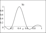
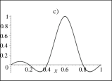
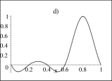
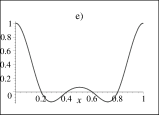
Figure 3. Graphs of optimal coefficients for $m=2$, $N=5$: a) $C([1],x)$, b) $C([2],x)$, c) $C([3],x)$, d) $C([4],x)$, e) $C([5],x)$.

Figure 4. Graphs of absolute errors for $m=2$, $N=5$: a) $|\sin(2\pi x)-P_{\varphi}(x)|$, b) $|B_{10}(x)-P_{\varphi}(x)|$.

The case $m=3$.

Figure 5. Graphs of optimal coefficients for $m=3$, $N=5$: a) $C([1],x)$, b) $C([2],x)$, c) $C([3],x)$, d) $C([4],x)$, e) $C([5],x)$.

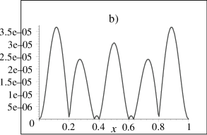
Figure 6. Graphs of absolute errors for $m=3$, $N=5$: a) $|\sin(2\pi x)-P_{\varphi}(x)|$, b) $|B_{10}(x)-P_{\varphi}(x)|$.

The case $m=4$.

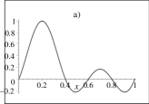
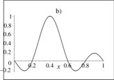
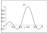
Figure 7. Graphs of optimal coefficients for $m=4$, $N=5$: a) $C([1],x)$, b) $C([2],x)$, c) $C([3],x)$, d) $C([4],x)$, e) $C([5],x)$.

Figure 8. Graphs of absolute errors for $m=4$, $N=5$: a) $|\sin(2\pi x)-P_{\varphi}(x)|$, b) $|B_{10}(x)-P_{\varphi}(x)|$.

From Figures 2,4,6,8 we can conclude that the absolute errors between given functions and optimal interpolation formula is decreasing as $m$ is increasing.

References

• [1] J.H.Ahlberg, E.N.Nilson, J.L.Walsh, The theory of splines and their applications, Mathematics in Science and Engineering, New York: Academic Press, 1967.
• [2] C. de Boor, A practical guide to splines, Springer-Verlag, 1978.
• [3] L.Schumaker, Spline functions: basic theory, J. Wiley, New-York, 1981.
• [4] P.-J.Laurent, Approximation and Optimization, Mir, Moscow, 1975, 496 p. (in Russian)
• [5] M.Attea, Hilbertian kernels and spline functions, Studies in Computational Matematics 4, C. Brezinski and L.Wuytack eds, North-Holland, 1992.
• [6] S.B.Stechkin, Yu.N.Subbotin, Splines in computational mathematics, Nauka, Moscow, 1976, 248 p. (in Russian)
• [7] V.A.Vasilenko, Spline-fucntions: Theory, Algorithms, Programs, Nauka, Novosibirsk, 1983, 216 p. (in Russian)
• [8] R.Arcangeli, M.C.Lopez de Silanes, J.J.Torrens, Multidimensional minimizing splines, Kluwer Academic publishers. Boston, 2004, 261 p.
• [9] M.I.Ignatev, A.B.Pevniy, Natural splines of many variables, Nauka, Leningrad, 1991. (in Russian)
• [10] N.P.Korneichuk, V.F.Babenko, A.A.Ligun, Extremal properties of polynomials and splines, Naukovo dumka, Kiev, 1992, 304 p. (in Russian)
• [11] G.Wahba, Spline models for observational data. CBMS 59, SIAM, Philadelphia, 1990.
• [12] R.L.Eubank, Spline smoothing and nonparametric regression. Marcel-Dekker, New-York, 1988.
• [13] P.J.Green and Silverman, Nonparametric regression and generalized linear models. A roughness penalty approach. Chapman and Hall, London, 1994.
• [14] A.Berlinet and C.Thomas-Agnan, Reproducing Kernel Hilbert Sapces in Probability and Statistics, Kluwer Academic Publisher, 2004.
• [15] J.C.Holladay, Smoothest curve approximation, Math. Tables Aids Comput. V.11. (1957) 223-243.
• [16] C. de Boor, Best approximation propertiesof spline functions of odd degree, J. Math. Mech. 12, (1963), pp.747-749.
• [17] I.J.Schoenberg, On trigonometric spline interpolation, J. Math. Mech. 13, (1964), pp.795-825.
• [18] M.Golomb, Approximation by periodic spline interpolants on uniform meshes, Journal of Approximation Theory, 1, (1968), pp. 26-65.
• [19] S.L.Sobolev, On Interpolation of Functions of $n$ Variables, in: Selected Works of S.L.Sobolev, Springer, 2006, pp. 451-456.
• [20] S.L.Sobolev, Formulas of Mechanical Cubature in $n$- Dimensional Space, in: Selected Works of S.L.Sobolev, Springer, 2006, pp. 445-450.
• [21] S.L.Sobolev, Introduction to the Theory of Cubature Formulas, Nauka, Moscow, 1974, 808 p.
• [22] S.L.Sobolev, V.L.Vaskevich. The Theory of Cubature Formulas. Kluwer Academic Publishers Group, Dordrecht (1997).
• [23] S.M.Nikolskii, Quadrature Formulas, Nauka, Moscow, 1988, (in Russian)
• [24] Kh.M.Shadimetov. The Discrete Analogue of the Differential Operator $d^{2m}/dx^{2m}$ ant Its Construction, Vopr. Vychisl. Prikl. Mat. 79, Tashkent, (1985), 22-35. arXiv:1001.0556 [NA.math]
• [25] S.L.Sobolev, A Difference Analogue of the Polyharmonic Equation, in: Selected Works of S.L.Sobolev, Springer, 2006, pp. 529-535.