On noise limited cellular networks

Abstract.

This paper introduces a general theoretical framework to analyze noise limited networks. More precisely, we consider two homogenous Poisson point processes of base stations and users. General model of radio signal propagation and effect of fading are also considered. The main difference of our model with respect to other existing models is that a user connects to his best servers but not necessarily the closest one. We provide general formula for the outage probability. We study functionals related to the SNR as well as the sum of these functionals over all users per cell. For the latter, the expectation and bounds on the variance are obtained.

1. Introduction

1.1. Motivation

Cellular network is a kind of radio network consisting of a number of fixed access points known as base stations and a large number of users (or mobiles). Each base station covers a geometrical region known as a cell and serve all users in this cell. Interference and noise are two factors annoying communications in cellular wireless networks. Noise is unavoidable and comes from natural sources. Interferences come from users and base stations. The use of recent technologies such as SDMA (spatial division multiple access) and MIMO (multiple input multiple output) can reduce significantly interferences so that we can hope that in a near future the impact of interferences will be negligible and noise will become the only factor harming the network. The best case is when interferences from other cells are perfectly canceled, the network is then said to be in noise limited regime. In this paper, we consider and introduce a framework to study this kind of network.

In existing literature, base stations (BS) locations are usually modeled as an ideal regular hexagonal lattice. In reality, base stations are irregularly located, especially in an urban area, and the cell radius is not the same for each BS. In this paper, we model the base station locations as an homogenous Poisson point process $\Pi_{B}$ of intensity $\lambda_{B}$. Such a model comes from stochastic geometry. It is sufficently versatile by changing $\lambda_{B}$ to cover a wide number of real situations and it is mathematically tractable. For an introduction to the usage of stochastic geometry for wireless networks performances, we refer to [8]. Theory and number of pertinent examples can be found in [1] and [2]. For all theoretical details, we refer the first opus.

To model cellular network cells, Voronoi tessellations are frequently used. It is based on the assumption that each user is served by the closest BS. Unfortunately, this is not always very accurate since in real life, a mobile connects to the best BS it can have, i.e., the BS which offers it the best Signal over Noise Ratio. The best BS is not always the closest because of the fading environment. In this paper, we analyze the impact of fading by considering that users are served by the base station providing the best signal power. The location of users in the plane are modeled as another homogenous Poisson point process $\Pi_{M}$ of intensity $\lambda_{M}$.

While ancient cellular networks such as GSM and GPRS provided only voice service and low data transmission rate, recent and emergent wireless cellular networks such as WIMAX or LTE offer higher data rate and other services requiring high throughput such as video calls. Each service requires a different level of signal to noise ratio (SNR). If the SNR does not reach a required threshold due to the radio condition, the service can not be established or may be interrupted. Such calls are said to be in outage. The outage probability is one of key measurement of the network performance. One of the aims of this paper is to determine the outage probability of noise limited network, or equivalently the distribution of SNR, which turns out to be equivalent to determine the distribution of the smallest path loss fading. In fact, there have been some works dealing with the outage probability of noise limited wireless network, but almost all of them consider the exponent path loss model. This paper provides a general formula for outage probability taking into account a more general model of path loss.

Once the distribution of SNR of a user is determined, the distribution of functionals related to SNR can be easily derived. In some situations, we have to study the distribution of the sum of a functional for all users in a cell. For example, in an OFDMA noise limited cellular system, the number of sub channels required for a user demanding a particular service depends on its SNR. If the total number of sub channels of all users in a cell excesses the number of available sub channels in this cell then at least one user is blocked. The probability of that to happen, sometimes called infeasibility probability, contains extremely important information on the performance of the network. Since it is often impossible to find the explicit probability distribution of additive functionals, we calculate the expectation, and bounds on the variance of such random variables.

This paper is organized as follows. In Section 2, we describe the model. In Section 3, we show that the path loss fading can be viewed as a Poisson point process on the real line and we provide a general formula for the outage probability. In Section 4, we calculate average capacity of a user and of a cell. We also compute upper and lower bounds for their variance as closed form expressions seem untractable. Section 5 illustrates the results obtained for some particular situations.

2. Model

2.1. System model

Consider a BS (base station) located at $y$ with transmission power $P$ and a mobile located at $x$. The mobile’s received signal has average power $L(y-x)P$ where $L$ is the path loss function. We assume that $L$ is measurable function on ${\mathbf{R}}^{2}$. The most used path loss function is the so-called path loss exponent model

$$L(z)=K|z|^{-\gamma},$$

where $|z|$ refers to the Euclidean norm of $z$. This function gives raise to nice closed formulas but is rather unrealistic: Close to the BS, the signal is infinitely amplified. A more realistic model is the modified path loss model given by:

$$L(z)=K\min\{R_{0}^{-\gamma},|z|^{-\gamma}\}$$

where $R_{0}$ is a reference distance and $K$ a constant depending on the environment. In addition to this deterministic large scale effect, we consider the fading effect, which is by essence random. The received signal power from a BS located at $y$ to a mobile unit (MU for short) located at $x$ is given by

$$P_{yx}=h_{y,\,x}L(y-x)P,$$

where $\{h_{y,\,x}\}_{x,y\in{\mathbf{R}}^{2}}$ are independent copies of a random variable $H$. Most used fading random models are log-normal shadowing and Rayleigh fading. The log-normal shadowing is such that $H$ is a log-normal random variable and we can write $H\sim 10^{G/10}$ where $G\sim\mathcal{N}(0,\sigma^{2})$. The Rayleigh fading is such that $H$ is an exponential random variable of parameter $\mu$. We can also consider the Rayleigh-Lognormal composite fading, in this case the fading is the product of the log-normal shadowing factor and the Rayleigh fading factor. It is worth noting that the log-normal shadowing usually improves the network performance while Rayleigh fading usually degrades performances.

We assume that once in the network, a mobile is attached to the BS that provides it the best signal strength. If the power received at this point is greater than some threshold $T$, we say that $x$ is covered. If $x$ is not covered by any BS then a MU at $x$ can not establish a communication and thus is said to be in outage. In the case of path loss exponent model with no fading ($H=\text{constant}$), the best BS for given mobile is always its nearest BS.

We assume that the point process of BSs $\Pi_{B}=\{y_{0},y_{1},...\}$ is an homogenous Poisson point process of intensity $\lambda_{B}$ on $\mathbf{R}^{2}$ and that users are distributed in the plane as a Poisson point process $\Pi_{M}=\{x_{0},x_{1},...\}$ of intensity $\lambda_{M}$.

To avoid any technical difficulty, from now on, we make the following assumptions:

Assumption 1.

Assume that:

1. All random variables $h_{yx}$ ($x,y\in\mathbf{R}^{2}$) are independent.

2. $H$ admits a probability density function $p_{H}$. Its complementary cumulative distributive function is denoted by $F_{H}$, i.e.,

   $$F_{H}(\beta)=P(H\geq\beta)=\int_{\beta}^{\infty}p_{H}(t)\text{ d}t>0.$$

3. Define $B(\beta)=\int_{R^{2}}F_{H}((L(z)\beta)^{-1})\text{ d}z$. Then, we have $0<B(\beta)<\infty$ for all $\beta>0$.

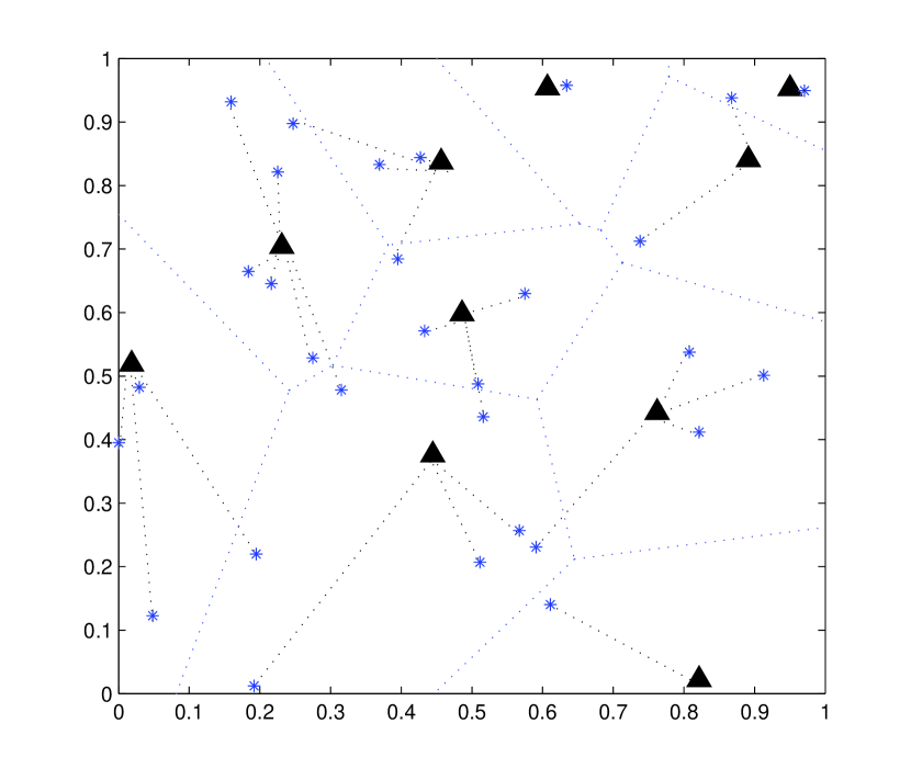
Figure 1. Triangles represent BS, plus represent MU. Dotted polygons are Voronoi cells induced by BS. A line between a BS and an MU means that the BS serves the MU. A mobile may be not served by the BS closest to it, due to fading.

3. Poisson point process of path loss fading

In this section, similarly to  [7], we show that the path loss fading process is a Poisson point process on the positive half of the real line.

For each location $x$ on $\mathbf{R}^{2}$, consider the path loss fading process $Sh^{x}=\{s_{i}^{x}\}_{i=0}^{\infty}$ where $s_{i}^{x}=(h_{y_{i}x}L(y-x))^{-1}$.

Proposition 1.

For any $x$, $Sh^{x}$ is a Poisson point process on ${\mathbf{R}}^{+}$ with intensity density $d\Lambda(t)=\lambda_{B}B^{\prime}(t)dt$. In addition, $B(0)=0$ and $B(\infty)=\infty$.

Proof.

Define the marked point process $\Pi_{B}^{x}=\{y_{i},h_{y_{i}x}\}_{i=0}^{\infty}$. It is a Poisson point process of intensity $\lambda_{B}dy\otimes f_{H}(t)dt$ because the marks are independent and identically distributed. Considering the probability kernel $p((z,t),A)=1_{\{(L(z)t)^{-1}\in A\}}$ for all Borel $A\subset\mathbf{R}^{+}$ and applying the displacement theorem ([1], theorem 1.3.9), we obtain that the point process $Sh^{x}$ is a Poisson point process of intensity

$$\Lambda(A)=\lambda_{B}\int_{R^{2}}\int_{R}1_{(\{L(z)t)^{-1}\in A\}}p_{H}(t)\text{ d}z\text{ d}t\cdotp$$

We now show that $\Lambda([0,\beta])=\lambda_{B}B(\beta)$. Indeed,

$$\Lambda([0,\beta]) = \lambda_{B}\int_{R^{2}}\int_{R}1_{\{t\geq(\beta L(z))^{-1}\}}p_{H}(t)\text{ d}z\text{ d}t$$

$$= \lambda_{B}\int_{R^{2}}F_{H}((\beta L(z))^{-1})\text{ d}z$$

$$= \lambda_{B}B(\beta)\cdotp$$

It is easy to see that $B(0)=0$ and $B(\infty)=\infty$. Finally $B(\beta)$ admits the derivative:

$$B^{\prime}(\beta)=\beta^{-2}\int_{R^{2}}\frac{1}{L(z)}p_{H}((\beta L(z))^{-1})\text{ d}z\cdotp$$

This concludes the proof. ∎

For any point $x$, we can reorder the points of $Sh^{x}.$ We denote ordered atoms of $Sh^{x}$ by $0\leq\xi_{0}^{x}<\xi_{1}^{x}<\ldots$. The CDF and PDF of $\xi^{x}_{m}$ are easily derived according to the property of Poisson point processes:

Corollary 1.

The complementary cumulative distribution function of $\xi_{m}^{x}$ is given by:

$$P(\xi_{m}^{x}>t)=e^{-\lambda_{B}B(t)}\sum_{i=0}^{m}\frac{(\lambda_{B}B(t))^{i}}{i!},$$

and its probability density function is given by

(1) $$p_{\xi_{m}^{x}}(t)=\frac{\lambda_{B}^{m+1}B^{\prime}(t)(B(t))^{m}}{m!}e^{-\lambda_{B}B(t)}\cdotp$$

Proof.

The event $(\xi_{m}^{x}>t)$ is equivalent to the event (in the interval $[0,t],$ there are at most $m$ points) and the number of points in this interval follows a Poisson distribution of mean $\lambda_{B}B(t)$. Thus, we have:

$$P(\xi_{m}^{x}>t)=e^{-\lambda_{B}B(t)}\sum_{i=0}^{m}\frac{(\lambda_{B}B(t))^{i}}{i!}\cdotp$$

The PDF is thus given by

$$p_{\xi_{m}^{x}}(t) = -\frac{\partial}{\partial t}P(\xi_{m}^{x}>t)$$

$$= -\lambda_{B}B^{\prime}(t)e^{-\lambda_{B}B(t)}$$

$$+\sum_{1}^{m}\lambda_{B}B^{\prime}(t)e^{-\lambda_{B}B(t)}\left(\frac{(\lambda_{B}B(t))^{i-1}}{(i-1)!}-\frac{(\lambda_{B}B(t))^{i}}{i!}\right)$$

$$= \frac{\lambda_{B}^{m+1}B^{\prime}(t)(B(t))^{m}}{m!}e^{-\lambda_{B}B(t)}\cdotp$$

The proof is thus complete. ∎

Corollary 2.

If $L(z)=K|z|^{-\gamma}$ then:

$$B(\beta)=C.\beta^{\frac{2}{\gamma}},$$

where $C=\pi K^{\frac{2}{\gamma}}E(H^{\frac{2}{\gamma}})$.

Proof.

The path loss function depends only on the distance from the BS to the user. By the change of variable $r=|z|$ and by integration by substitution, we have:

$$B(\beta) = 2\pi\int_{0}^{\infty}\int_{0}^{\infty}r1_{\{tK\beta\geq r^{\gamma}\}}p_{H}(t)\text{ d}r\text{ d}t$$

$$= 2\pi\int_{0}^{\infty}p_{H}(t)\text{ d}t\int_{0}^{(tK\beta)^{1/\gamma}}r\text{ d}r$$

$$= \pi(K)^{\frac{2}{\gamma}}\beta^{\frac{2}{\gamma}}\int_{0}^{\infty}p_{H}(t)t^{\frac{2}{\gamma}}\text{ d}t$$

$$= \pi(K)^{\frac{2}{\gamma}}E(H^{\frac{2}{\gamma}})\beta^{\frac{2}{\gamma}}\cdotp$$

Hence the result. ∎

Remark that this result can also be derived from [7]. We observe that the distribution of the point process $Sh^{x}$ does depend only on $E(H^{\frac{2}{\gamma}})$ but not on the distribution of fading $H$ itself. This phenomenon can be explained as in [9](page 159). If the fading is log-normal shadowing, i.e $H\sim 10^{G/10}$ where $G\sim\mathcal{N}(0,\sigma^{2})$ then $E(H^{\frac{2}{\gamma}})=e^{\frac{2\sigma_{1}^{2}}{\gamma^{2}}}$ where $\sigma_{1}=\frac{\ln(10)\sigma}{10}$. If the fading is Rayleigh fading, i.e $H\sim\exp(\mu)$ then $E(H^{\frac{2}{\gamma}})=\Gamma(\frac{2}{\gamma}+1,0)\mu^{-\frac{2}{\gamma}}$ where $\Gamma(a,b)=\int_{b}^{\infty}t^{a-1}e^{-t}\text{ d}t$ is the upper incomplete gamma function.

Similarly to the distance to $m$-th nearest BS (which can be found in [11]), the distribution of $m$-th less strong path loss fading $\xi_{m}^{x}$ can be characterized as follows:

Corollary 3.

If $L(z)=K|z|^{-\gamma}$, $\xi_{m}^{x}$ is distributed according to the generalized Gamma distribution:

$$p_{\xi_{m}^{x}}(t)=\frac{2}{\gamma}(\lambda_{B}C)^{m+1}t^{\frac{2}{\gamma}(m+1)}\frac{e^{-\lambda_{B}Ct^{\frac{2}{\gamma}}}}{m!}\cdotp$$

Proof.

This is a consequence of Proposition 1 and Lemma 2. ∎

We can also investigate more general and realistic path loss model.

Corollary 4.

If $L(z)=K\min\{R_{0}^{-\gamma},|z|^{-\gamma}\}$ then:

(2) $$B(\beta)=C_{1}\beta^{\frac{2}{\gamma}}\int_{\frac{R_{0}^{\gamma}}{\beta K}}^{\infty}t^{\frac{2}{\gamma}}p_{H}(t)\text{ d}t,$$

where $C_{1}=\pi K^{\frac{2}{\gamma}}$. In addition, we have:

(3) $$B^{\prime}(\beta)=\frac{2}{\gamma}\beta^{-1}B(\beta)+\pi R_{0}^{2}p_{H}\left(\frac{R_{0}^{\gamma}}{K\beta}\right)\cdotp$$

If the fading is lognormal shadowing $H\sim 10^{G/10}$ where $G\sim\mathcal{N}(0,\sigma^{2})$ then we have:

$$B(\beta)=C_{1}\beta^{\frac{2}{\gamma}}e^{(\frac{2\sigma_{1}}{\gamma})^{2}}Q\left(\frac{-\ln\beta-\ln(KR_{0}^{-\gamma})}{\sigma_{1}}-\frac{2\sigma_{1}}{\gamma}\right),$$

where $Q(a)=\frac{1}{\sqrt{2\pi}}\int_{a}^{\infty}e^{-u^{2}/2}\text{ d}u$ is the Q-function and $\sigma_{1}=\frac{\sigma\ln 10}{10}$. If the fading is Rayleigh $H\sim\exp(\mu)$ then

$$B(\beta)=C_{1}\left(\frac{\beta}{\mu}\right)^{\frac{2}{\gamma}}\Gamma\left(1+\frac{2}{\gamma},\frac{\mu R_{0}^{\gamma}}{K\beta}\right).$$

Proof.

Similarly to the path loss exponent model case, we have:

$$B(\beta) = 2\pi\int_{0}^{\infty}rF_{H}((\max\{R_{0},r\})^{-\gamma}(K\beta)^{-1})\text{ d}r$$

$$= 2\pi\int_{0}^{R_{0}}rF_{H}(R_{0}^{-\gamma}(K\beta)^{-1})\text{ d}r+2\pi\int_{R_{0}}^{\infty}rF_{H}(R_{0}^{-\gamma}(K\beta)^{-1})\text{ d}r$$

$$= \pi R_{0}^{2}F_{H}(R_{0}^{\gamma}(K\beta)^{-1})+2\pi\int_{\frac{R_{0}^{\gamma}}{\beta K}}^{\infty}p_{H}(t)\text{ d}t\int_{R_{0}}^{(tK\beta)^{1/\gamma}}r\text{ d}r$$

$$= C_{1}\beta^{\frac{2}{\gamma}}\int_{\frac{R_{0}^{\gamma}}{K\beta}}^{\infty}t^{\frac{2}{\gamma}}p_{H}(t)\text{ d}t\cdotp$$

We then obtain Equation (2). Now differentiate the two sides of that equation to get:

$$B^{\prime}(\beta) = \frac{2}{\gamma}C_{1}\beta^{\frac{2}{\gamma}-1}\int_{\frac{R_{0}^{\gamma}}{\beta K}}^{\infty}t^{\frac{2}{\gamma}}p_{H}(t)\text{ d}t+\frac{C_{1}R_{0}^{2}}{K^{\frac{2}{\gamma}}}p_{H}\left(\frac{R_{0}^{\gamma}}{K\beta}\right)$$

$$= \frac{2}{\gamma}\beta^{-1}B(\beta)+\pi R_{0}^{2}p_{H}\left(\frac{R_{0}^{\gamma}}{K\beta}\right).$$

That yields Equation (3). In the case of lognormal shadowing we have:

$$B(\beta) = C_{1}\beta^{\frac{2}{\gamma}}\int_{\frac{R_{0}^{\gamma}}{K\beta}}^{\infty}\frac{1}{\sqrt{2\pi\sigma_{1}^{2}}t}t^{\frac{2}{\gamma}}e^{-\frac{(\ln t)^{2}}{2\sigma_{1}^{2}}}\text{ d}t$$

$$= C_{1}\beta^{\frac{2}{\gamma}}\int_{\ln\frac{R_{0}^{\gamma}}{K\beta}}^{\infty}\frac{1}{\sqrt{2\pi\sigma_{1}^{2}}}e^{\frac{2u}{\gamma}}e^{-\frac{u^{2}}{2\sigma_{1}^{2}}}\text{ d}u$$

$$= C_{1}\beta^{\frac{2}{\gamma}}e^{(\frac{2\sigma_{1}}{\gamma})^{2}}\int_{\ln\frac{R_{0}^{\gamma}}{K\beta}}^{\infty}\frac{1}{\sqrt{2\pi\sigma_{1}^{2}}}e^{-\frac{(u-\frac{2\sigma_{1}^{2}}{\gamma})^{2}}{2\sigma_{1}^{2}}}\text{ d}u$$

$$= C_{1}\beta^{\frac{2}{\gamma}}e^{(\frac{2\sigma_{1}}{\gamma})^{2}}Q\left(\frac{-\ln\beta-\ln(KR_{0}^{-\gamma})}{\sigma_{1}}-\frac{2\sigma_{1}}{\gamma}\right)\cdotp$$

In the case of Rayleigh fading we have:

$$B(\beta) = C_{1}\beta^{\frac{2}{\gamma}}\int_{\frac{R_{0}^{\gamma}}{K\beta}}^{\infty}t^{\frac{2}{\gamma}}\mu e^{-\mu t}\text{ d}t$$

$$= C_{1}\left(\frac{\beta}{\mu}\right)^{\frac{2}{\gamma}}\Gamma\left(1+\frac{2}{\gamma},\frac{\mu R_{0}^{\gamma}}{K\beta}\right),$$

by a change of variables. Hence the results. ∎

Corollary 5.

The number of BS covering a point $x$ is distributed according to the Poisson distribution of parameter $\lambda_{B}B(T)$. In particular, the outage probability given a threshold $T$ is

$$P(\xi_{0}^{x}>T)=e^{-\lambda_{B}B(T)}.$$

Proof.

The path loss fading $Sh^{x}$ is a Poisson point process on ${\mathbf{R}}^{+}$ with intensity $\lambda_{B}B^{\prime}(t)\text{ d}t$, so the number of point on the interval $(0,T)$ is distributed according to Poisson distribution of parameter $\lambda_{B}B(T)$. ∎

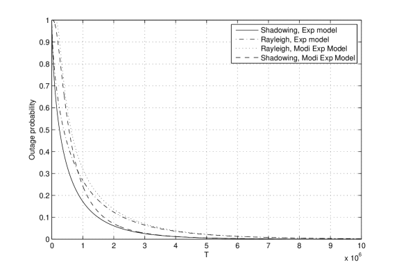
Figure 2. Comparison of outage probability between propagation models. For lognormal shadowing $\sigma=4(dB)$, for Rayleigh fading $\mu=1$; $K=10^{-2}$, $\gamma=2.8$.

Figure 2 represents the outage probability for different models of fading. This shows that the curves of modified path loss exponent model is generally higher than those of path loss exponent model but they are very close in the low outage region.

4. Capacity

In this section, we calculate the mean of any capacity function of a user. Remark that since the system is spatially stationary the statistic of the path loss fading and the capacity of a user does not depend on his position. Since the PDF and the CDF of the path loss fading $\xi^{x}_{0}$ have been already calculated in Proposition 1, the mean of a capacity function of a user follows immediately. In particular:

Theorem 2.

The average capacity per user is

(4) $$E(f(\xi_{0}^{x}))=\lambda_{B}\int_{0}^{\infty}B^{\prime}(\beta)e^{-\lambda_{B}B(\beta)}f(\beta)\text{ d}\beta\cdot$$

In the case of path loss exponent model $L(z)=K|z|^{-\gamma}$, we have:

(5) $$E(f(\xi_{0}^{x}))=\mathcal{L}_{\widetilde{f}}(\lambda_{B}C)$$

where $\mathcal{L}_{g}(s)=\int_{0}^{\infty}e^{-st}g(t)\text{ d}t$ is the Laplace transform of the capacity function $g$ and $\widetilde{f}(t)=f(t^{\frac{\gamma}{2}})$.

Proof.

Equation (4) comes from Proposition 1. If the path loss exponent model is considered, then we have:

$$E(f(\xi_{0}^{x})) =\lambda_{B}\int_{0}^{\infty}\frac{2C}{\gamma}\beta^{\frac{2}{\gamma}-1}e^{-\lambda_{B}C\beta^{\frac{2}{\gamma}}}f(\beta)\text{ d}\beta$$

$$=\int_{0}^{\infty}e^{-\lambda_{B}C\beta_{1}}f(\beta_{1}^{\frac{\gamma}{2}})\text{ d}\beta_{1}$$

by the change of variable $\beta_{1}=\beta^{\frac{\gamma}{2}}$. ∎

The statistic of the cell capacity $S_{o}(f)$ is more difficult to analyze. In this section, we calculate its mean $m(f)$ and lower bound and upper bound of its variance $v(f)$. We state the following lemma, which is straightforward due to Assumption 1 but still useful:

Lemma 3.

Given a fixed configuration $\Pi_{B}$ of BSs, the Poisson point processes of path loss fading $Sh^{x}$ and $Sh^{y}$ are independent for any two different points $x,\,y$.

Lemma 4.

Let $z=y-x$. The PDF of $s_{yx}$ is given by

$$p_{s_{yx}}(t)=\frac{1}{l(z)t^{2}}p_{H}\left(\frac{1}{L(z)t}\right).$$

Proof.

We have

$$P(s_{yx}<t) = P(h_{yx}>\frac{1}{L(z)t})$$

$$= F_{H}\left(\frac{1}{L(z)t}\right).$$

The density probability function is then

$$p_{s_{yx}}(t)=\frac{1}{L(z)t^{2}}p_{H}\left(\frac{1}{L(z)t}\right).$$

∎

Theorem 5.

The expectation of the cell capacity of the typical BS is

(6) $$m(f)=\lambda_{M}\int_{0}^{\infty}B^{\prime}(\beta)e^{-\lambda_{B}B(\beta)}f(\beta)\text{ d}\beta\cdot$$

In the case of path loss exponent model $L(z)=K|z|^{-\gamma}$, we have:

(7) $$m(f)=\frac{\lambda_{M}}{\lambda_{B}}\mathcal{L}_{\widetilde{f}}(\lambda_{B}C)\cdot$$

Proof.

Given a fixed configuration of BSs $\Pi_{B}$, the random variables $1(s_{ox}<\xi_{0}^{x})f(s_{ox})$ obtained from all $x\in\mathbf{R}^{2}$ are independent. Thus, the marked point process $\tilde{\Pi}_{M}=(x_{i},1(s_{ox_{i}}<\xi_{0}^{x_{i}})f(s_{ox_{i}}))$ is a Poisson point process. Using the Campbell theorem we have:

$$E(S_{o}(f)\mid\Pi_{B})=\lambda_{M}\int_{\mathbf{R}^{2}}E\left(1(s_{ox}<\xi_{0}^{x})f(s_{ox})\mid\Pi_{B}\right)\text{ d}x\cdot$$

As a consequence,

$$E(S_{o}(f)) =E\left(\lambda_{M}\int_{\mathbf{R}^{2}}E(1(s_{ox}<\xi_{0}^{x})f(s_{ox})\mid\Pi_{B})\text{ d}x\right)$$

$$=\lambda_{M}\int_{\mathbf{R}^{2}}E\left(1(s_{ox}<\xi_{0}^{x})f(s_{ox})\right)\text{ d}x\cdot$$

In virtue of Lemma 4, Proposition 1 and Collary 1, we have:

$$E(S_{o}(f)) =\lambda_{M}\int_{\mathbf{R}^{2}}E(1(s_{ox}<\xi_{0}^{x})f(s_{ox}))\text{ d}x$$

$$=\lambda_{M}\int_{\mathbf{R}^{2}}\int_{0}^{\infty}p_{s_{ox}}(t)P(t<\xi_{0}^{x})f(t)\text{ d}t\text{ d}x$$

$$=\lambda_{M}\int_{0}^{\infty}f(t)e^{-\lambda_{B}B(t)}\text{ d}t\int_{\mathbf{R}^{2}}\frac{\partial F_{H}}{\partial t}\left(\frac{1}{L(x)t}\right)\text{ d}x$$

$$=\lambda_{M}\int_{0}^{\infty}f(t)e^{-\lambda_{B}B(t)}\text{ d}t\frac{\partial}{\partial t}\left(\int_{R^{2}}F(\frac{1}{L(x)t})\text{ d}x\right)$$

$$=\lambda_{M}\int_{0}^{\infty}f(t)e^{-\lambda_{B}B(t)}B^{\prime}(t)\text{ d}t\cdot$$

For the case of path loss exponent model, Equation 7 follows easily. This completes the proof. ∎

Equation (6) has the following interpretation: the mean cell capacity is the product of the mean number of users per cell and the mean capacity per user.

Theorem 6.

Given two capacity functions $f,g$ we have :

(8) $$\operatorname{\text{cov}}(S_{o}(f),S_{o}(g))\geq m(f.g)\cdot$$

In particular,

$$\operatorname{\text{var}}(S_{o}(f))\geq m(f^{2}).$$

Proof.

For simplicity, let $\beta_{x}=s_{ox}1(s_{ox}<\xi_{0}^{x})$ and $f(0)=0,g(0)=0$, we have :

$$\operatorname{\text{cov}}(S_{o}(f)S_{o}(g)) =E(\operatorname{\text{cov}}(S_{o}(f),S_{o}(g)\mid\Pi_{B}))$$

$$+E(E(S_{o}(f)\mid\Pi_{B})E(S_{o}(g)\mid\Pi_{B}))-E(S_{o}(f))E(S_{o}(g))$$

$$=T_{1}+T_{2}-T_{3}\cdot$$

It is clear that

$$T_{3}=m(f)m(g)\cdot$$

Consider the first term. Remind that we have assumed that all random fading $\{h_{yx}\}_{y,x\in\mathbf{R}^{2}}$ are independent, so given a fixed configuration $\Pi_{B}$ of BSs, the random variables $\{\beta_{x}\}_{x\in\mathbf{R}^{2}}$ are independent. Hence by Campbell formula we have:

$$T_{1} = \lambda_{M}E\int_{\mathbf{R}^{2}}E(f(\beta_{x})g(\beta_{x})\mid\Pi_{B})\text{ d}x$$

$$= \lambda_{M}\int_{\mathbf{R}^{2}}E(E(f(\beta_{x})g(\beta_{x})\mid\Pi_{B}))\text{ d}x$$

$$= \lambda_{M}\int_{\mathbf{R}^{2}}E(f(\beta_{x})g(\beta_{x}))\text{ d}x$$

$$= m(f.g)\cdot$$

Now consider the second term

$$T_{2}=\lambda_{M}^{2}E\left(\int_{\mathbf{R}^{2}}E(f(\beta_{x})\mid\Pi_{B})\text{ d}x\int_{R^{2}}E(g(\beta_{x})\mid\Pi_{B})\text{ d}x\right)\\ \begin{aligned} &=\lambda_{M}^{2}E\left(\int_{\mathbf{R}^{2}}\int_{\mathbf{R}^{2}}E(f(\beta_{x})\mid\Pi_{B})E(g(\beta_{y})\mid\Pi_{B})\text{ d}x\text{ d}y\right)\\ &=\lambda_{M}^{2}\int_{\mathbf{R}^{2}}\int_{\mathbf{R}^{2}}E\left(E(f(\beta_{x})\mid\Pi_{B})E(g(\beta_{y})\mid\Pi_{B})\right)\text{ d}x\text{ d}y\\ &=\lambda_{M}^{2}\int_{\mathbf{R}^{2}}\int_{\mathbf{R}^{2}}E(f(\beta_{x}))E(g(\beta_{y}))\text{ d}x\text{ d}y\\ &=\lambda_{M}^{2}\int_{\mathbf{R}^{2}}\int_{\mathbf{R}^{2}}\int_{0}^{\infty}\int_{0}^{\infty}P(s_{ox}<\xi_{0}^{x},s_{oy}<\xi_{0}^{y}\mid s_{ox}=t_{1},s_{oy}=t_{2})\times\end{aligned}\\ \times f(t_{1})g(t_{2})p_{s_{ox}}(t_{1})p_{s_{oy}}(t_{2})\text{ d}t_{1}\text{ d}t_{2}\text{ d}x\text{ d}y\cdot$$

by remarking that $\beta_{x}$ and $\beta_{y}$ are independent if $x\neq y$ (Lemma 3). We will prove that if $x\neq y$:

$$P(s_{ox}<\xi_{0}^{x},s_{oy}<\xi_{0}^{y}\mid s_{ox}=t_{1},s_{oy}=t_{2})\geq\\ P(s_{ox}<\xi_{0}^{x}\mid s_{ox}=t_{1})P(s_{oy}<\xi_{0}^{y}\mid s_{oy}=t_{2})$$

Consider the marked point process $\Pi_{B}^{x,y}=\{y_{i},h_{y_{i}x},h_{y_{i}y})\}$. Since the marks are independent, it is a Poisson point process on $\mathbf{R}^{4}$ with intensity

$$m_{a}^{x,u_{1},u_{2}}(\text{ d}y,du_{1},du_{2})=\lambda_{M}\text{ d}y\otimes p_{H}(u_{1})du_{1}\otimes p_{H}(u_{2})du_{2}\cdot$$

Consider two sets

$$A_{1}=\{(y,u_{1},u_{2}):L(y)u_{1}\geq t_{1}^{-1}\}$$

and

$$A_{2}=\{(y,u_{1},u_{2}):L(y)u_{2}\geq t_{2}^{-1}\},$$

we have:

$$P(s_{ox}<\xi_{0}^{x},s_{oy}<\xi_{0}^{y}\mid s_{ox}=t_{1},s_{oy}=t_{2})=P(\Pi_{B}^{x,y}(A_{1}\cup A_{2})=\emptyset)\\ \begin{aligned} &=e^{-m_{a}^{x,y}(A_{1}\cup A_{2})}\\ &\geq e^{-m_{a}^{x,y}(A_{1})-m_{a}^{x,y}(A_{2})}\\ &=P(\Pi_{B}^{x,y}(A_{1})=\emptyset)P(\Pi_{B}^{x,y}(A_{2})=\emptyset)\\ &=P(s_{ox}<\xi_{0}^{x}\mid s_{ox}=t_{1})P(s_{oy}<\xi_{0}^{y}\mid s_{oy}=t_{2})\cdot\end{aligned}$$

Thus,

$$T_{2} \geq\lambda_{M}^{2}\int_{\mathbf{R}^{2}}\int_{\mathbf{R}^{2}}\int_{0}^{\infty}\int_{0}^{\infty}P(s_{ox}<\xi_{0}^{x}\mid s_{ox}=t_{1})P(s_{oy}<\xi_{0}^{y}\mid s_{oy}=t_{2})\times$$

$$\ \ \ \ \times f(t_{1})g(t_{2})p_{s_{ox}}(t_{1})p_{s_{oy}}(t_{2})\text{ d}t_{1}\text{ d}t_{2}\text{ d}x\text{ d}y$$

$$=m(f)m(g)\cdot$$

The result follows. ∎

Theorem 7.

For $f$ and $g$ two capacity functions, we have:

$$\operatorname{\text{cov}}(S_{o}(f),S_{o}(g))\leq m(f.g)+m(f)n(g)-m(f)m(g)$$

where

(9) $$n(f)=\lambda_{M}\int_{0}^{\infty}B^{\prime}(t)f(t)\text{ d}t\cdot$$

Proof.

We continue the proof of Theorem 6, we have to prove that

$$T_{2}\leq m(f)n(g)\cdot$$

Indeed,

$$P(s_{ox}<\xi_{0}^{x},s_{oy}<\xi_{0}^{y}\mid s_{ox}=t_{1},s_{oy}=t_{2})\leq P(s_{ox}<\xi_{0}^{x}\mid s_{ox}=t_{1}),$$

thus,

$$T_{2} \leq\lambda_{M}^{2}\int_{\mathbf{R}^{2}}\int_{\mathbf{R}^{2}}\int_{0}^{\infty}\int_{0}^{\infty}P(s_{ox}<\xi_{0}^{x}\mid s_{ox}=t_{1})\times$$

$$\ \ \ \ \ \times f(t_{1})g(t_{2})p_{s_{ox}}(t_{1})p_{s_{oy}}(t_{2})\text{ d}t_{1}\text{ d}t_{2}\text{ d}x\text{ d}y$$

$$\leq m(f)\int_{0}^{\infty}g(t_{2})\int_{{\mathbf{R}}^{2}}\frac{\partial F_{H}}{\partial t}(\frac{1}{L(x)t})\text{ d}x\text{ d}t_{2}$$

$$=m(f)n(g)\cdot$$

Hence the result. ∎

5. Examples

5.1. Number of users in a cell

For $f_{0}(t)=1$, the random variable $n_{o}:=S(f_{0})=\sum_{i=0}^{\infty}1(x_{i}\in C_{o})$ represents the number of users who view $o$ as the best server, and thus will be served by $o$.

$$E(n_{o}) = \lambda_{M}\int_{0}^{\infty}B^{\prime}(\beta)e^{-\lambda_{B}B(\beta)}d\beta$$

$$= \frac{\lambda_{M}}{\lambda_{B}}\cdot$$

The mean number of users served by a BS is $\frac{\lambda_{M}}{\lambda_{B}}$ which is easily interpreted. We rewrite the formula (6) by

$$E(S_{o}(f))=\frac{\lambda_{M}}{\lambda_{B}}E(f(\xi_{0}^{x})).$$

Again this is easily interpreted. The average sum rate is the product of the average user per cell and the average per user.

Now apply Theorem 6, we get that

$$\operatorname{\text{var}}(n_{o})\geq m(1)=\frac{\lambda_{M}}{\lambda_{B}}\cdotp$$

We can not apply Theorem 7 because $n(f_{0})=\lambda_{M}\int_{0}^{\infty}B^{\prime}(t)\text{ d}t=\infty$.

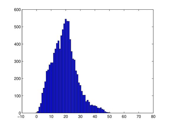
Figure 3. Histogram of $n_{o}$

5.2. Number of users in outage in a cell

Consider $f_{1}(t)=1(t>T)$, then $S_{o}(f_{1})$ is the number of users in outage in the typical cell. We have

$$m(f_{1}) =\lambda_{M}\int_{T}^{\infty}B^{\prime}(\beta)e^{-\lambda_{B}B(\beta)}d\beta$$

$$=\frac{\lambda_{M}}{\lambda_{B}}e^{-\lambda_{B}B(T)},$$

and

$$v(f_{1})\geq\frac{\lambda_{M}}{\lambda_{B}}e^{-\lambda_{B}B(T)}\cdot$$

Note that again, we can not apply Theorem 7 as $n(f_{1})=\lambda_{M}\int_{T}^{\infty}B^{\prime}(t)\text{ d}t$ is infinite.

5.3. Number of covered users in a cell

Consider $f_{2}(t)=1(t\leq T)$, then $S(f_{2})$ represents the number of covered users in the typical cell. We have:

$$m(f_{2}) =\lambda_{M}\int_{0}^{T}B^{\prime}(\beta)e^{-\lambda_{B}B(\beta)}d\beta$$

$$=\frac{\lambda_{M}}{\lambda_{B}}\left(1-e^{-\lambda_{B}B(T)}\right),$$

$$v(f_{2})\geq\frac{\lambda_{M}}{\lambda_{B}}\left(1-e^{-\lambda_{B}B(T)}\right),$$

and

$$v(f_{2})\leq\frac{\lambda_{M}}{\lambda_{B}}e^{-\lambda_{B}B(T)}+\frac{\lambda_{M}^{2}}{\lambda_{B}^{2}}e^{-\lambda_{B}B(T)}\left(\lambda_{B}B(T)-1+e^{-\lambda_{B}B(T)}\right)\cdot$$

5.4. Total bit rate of a cell

We now consider the piecewise constant function $f_{3}(t)=\sum_{1}^{n}1(T_{i}\leq t<T_{i+1})c_{i}$ with $0<T_{1}<T_{2}<...<T_{n}<T_{n+1}$ and $T_{n+1}$ can be infinite. If $f_{3}$ is the function that represents the actual bit rate then $S_{o}(f_{3})$ represents the total bit rates of all users in the cell. We have:

$$m(f_{3}) = \lambda_{M}\int_{0}^{\infty}B^{\prime}(\beta)e^{-\lambda_{B}B(\beta)}\sum_{1}^{n}1(T_{i}\leq\beta<T_{i+1})c_{i}d\beta$$

$$= \lambda_{M}\sum_{i=1}^{n}c_{i}\left(e^{-\lambda_{B}B(T_{i})}-e^{-\lambda_{B}B(T_{i+1})}\right)\cdot$$

$$v(f_{3}) \geq \lambda_{M}\sum_{i=1}^{n}c_{i}^{2}\left(e^{-\lambda_{B}B(T_{i})}-e^{-\lambda_{B}B(T_{i+1})}\right)\cdot$$

$$v(f_{3}) \leq \lambda_{M}\sum_{i=1}^{n}c_{i}^{2}\left(e^{-\lambda_{B}B(T_{i})}-e^{-\lambda_{B}B(T_{i+1})}\right)+$$

$$+\left(\frac{\lambda_{M}}{\lambda_{B}}\right)^{2}\sum_{i=1}^{n}\left(e^{-\lambda_{B}B(T_{i})}-e^{-\lambda_{B}B(T_{i+1})}\right)\times$$

$$\times\sum_{i=1}^{n}\left(\lambda_{B}B(T_{i+1})-\lambda_{B}B(T_{i})-e^{-\lambda_{B}B(T_{i})}+e^{-\lambda_{B}B(T_{i+1})}\right)\cdot$$

5.5. Discussion on the distribution of $S_{o}(f)$

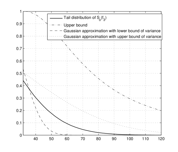
Figure 4. Tail distribution of $S_{o}(f_{3})$

The distribution of $S_{o}(f)$ does not behave like a Gaussian distribution even in the limit regimes. Take, for example, the histogram of $n_{o}=S_{o}(f_{0})$ and that of $S_{o}(f_{3})$ which are shown in figures 3 and 5 respectively. For the case of no fading, $H=$ constant, in [6] the author found some approximative but not reliable bounds of the distribution of $S_{o}(f)$ for equivariant functions $f$ but no approximation or bounds is found for general capacity functions. In addition, no closed expression is found for the Laplace transform of functional $S_{o}(f)$. In our case where the fading is considered, this is expected to be more challenging.

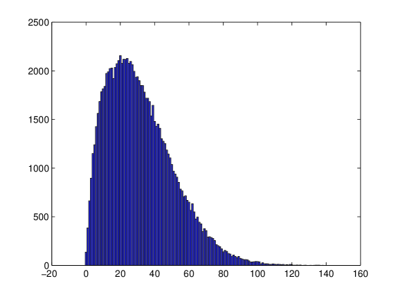
Figure 5. A typical histogram of $S_{o}(f_{3})$

We can find an upper bound for the tail distribution by Chebyshev’s inequality:

$$P(S_{o}(f)>m(f)+t) \leq \frac{v(f)}{v(f)+t^{2}}$$

$$\leq \frac{m(f^{2})+m(f)n(f)-(m(f))^{2}}{m(f^{2})+m(f)n(f)-(m(f))^{2}+t^{2}}$$

The above inequality provides a robust upper bound for the tail distribution and valid for all capacity function $f$. However the gap is large (Figure 4). It is well known that other types of concentration inequality based on Chernoff bound can give better bound. In this direction, [10], [5] and [12] provide concentration inequalities that apply for functional related to one PPP. These inequalities can not be directly applied in our case because our target is a functional related to two independent PPPs. Actually we can combine the two independent PPPs into one united PPP by the independent marking theorem. Unfortunately the functional $S_{o}(f)$ of the united PPP does not satisfy the required conditions for the concentration inequalities neither on [10], [12] nor on [5]. But we believe that similar techniques used in these references can be used to derive a upper bound the tail distribution of $S_{o}(f)$.

6. Conclusion

In this paper we introduce a general model to evaluate the outage probability and the capacity of wireless noise limited network. It is in fact an extension of models introduced in series of papers [4], [3], [6]. The main difference is that we take into account the effect of fading, and that we assume that a user connects to the BS with strongest signal rather than the closest one. We first show that for a particular user, the path loss fading process from all BSs seen from this user is a Poisson point process in the positive half line. We find explicit expression for the outage probability, the expectation of capacity of a user, and the expectation of the cell capacity of the typical BS $S_{o}(f)$. We find the lower bound and upper bound for the variance of the cell capacity. We consider general model for path loss and fading. The results presented in this paper actually generalizes the results on [6]. Possible further research is to find a way to compute the distribution of $S_{o}(f)$.

References

- [1] F. Baccelli and B. Blaszczyszyn. Stochastic geometry and wireless networks, volume 1: Theory. Foundations and Trends in Networking, 3(3-4):249–449, 2009.
- [2] F. Baccelli and B. Blaszczyszyn. Stochastic geometry and wireless networks, volume 2: Applications. Foundations and Trends in Networking, 4(1-2):1–312, 2009.
- [3] F. Baccelli, M. Klein, M. Lebourges, and S. Zuyev. Géométrie aléatoire et architecture de réseaux. Annals of Telecommunications, 51:158–179, 1996.
- [4] F. Baccelli, M. Klein, M. Lebourges, and S. Zuyev. Stochastic geometry and architecture of communication networks. Telecommunication Systems, 7:209–227, 1997.
- [5] L. Decreusefond, A. Joulin, and N. Savy. Upper bounds on Rubinstein distances on configuration spaces and applications. Communications on stochastic analysis, 2010.
- [6] S. Foss and S. Zuyev. On a voronoi aggregative process related to a bivariate poisson process. pages 965–981, 1996.
- [7] M. Haenggi A Geometric Interpretation of Fading in Wireless Networks: Theory and Applications. IEEE Transaction on Information Theory, 54(12):5500–5510, December 2008.
- [8] M. Haenggi, J. G. Andrews, F. Baccelli, O. Dousse, and M. Franceschetti. Stochastic geometry and random graphs for the analysis and design of wireless networks. IEEE Journal of Selected Areas in Communications, 27:1029–1046, September 2009.
- [9] M. Haenggi and R. K. Ganti. Interference in Large Wireless Networks. Foundations and Trends in Networking, 3(2):127–248, 2008.
- [10] C. Houdré and N. Privault. Concentration and deviation inequalities in infinite dimensions via covariance representations. Bernoulli, 8(6):697–720, 2002.
- [11] S. Srinivasa and M. Haenggi. Distance Distributions in Finite Uniformly Random Networks: Theory and Applications. IEEE Transactions on Vehicular Technology, 59(2):940–949, February 2010.
- [12] L. Wu. A new modified logarithmic Sobolev inequality for Poisson point processes and several applications. Probability Theory and Related Fields, 118(3):427–438, 2000.