Evidence for coherent quantum phase-slips across a Josephson junction array

Abstract

Superconducting order in a sufficiently narrow and infinitely long wire is destroyed at zero temperature by quantum fluctuations, which induce $2\pi$ slips of the phase of the order parameter. However, in a finite-length wire coherent quantum phase-slips would manifest themselves simply as shifts of energy levels in the excitations spectrum of an electrical circuit incorporating this wire. The higher the phase-slips probability amplitude, the larger are the shifts. Phase-slips occurring at different locations along the wire interfere with each other. Due to the Aharonov-Casher effect, the resulting full amplitude of a phase-slip depends on the offset charges surrounding the wire. Slow temporal fluctuations of the offset charges make the phase-slips amplitudes random functions of time, and therefore turn energy levels shifts into linewidths. We experimentally observed this effect on a long Josephson junction array acting as a “slippery” wire. The slip-induced linewidths, despite being only of order $100~{}\mathrm{kHz}$, were resolved from the flux-dependent dephasing of the fluxonium qubit.

I Introduction

The basic notion of superconductivity as a cooperative phenomenon is the superconducting order parameter. It is a continuous and complex single-valued function of coordinates, commonly referred to as the macroscopic wave functionGinzburgLandau1950 . The electronic condensate of a superconductor can move without friction, manifesting itself as a current without Joule dissipation. The density of a non-dissipative current (supercurrent) is proportional to the phase gradient of the macroscopic wave function; its amplitude is constant along the wire. At fixed gradient, phase is a linear function of the coordinate along the wire. For a long wire, the phase difference between the wire’s ends may exceed, by many orders of magnitude, the basic period $2\pi$. This behavior is inconsistent with the thermodynamics of a superconductor, as its free energy is a $2\pi$-periodic function of the phase difference. Thus, the equilibrium current reaches a maximum at a phase difference of $\pi$ and then oscillates with a further increase of phase difference.

In a narrow wire (thinner than the coherence length), the adjustment of the supercurrent to the equilibrium value is achieved by the transient processes of $2\pi$ phase-slips (PS) of the macroscopic wave function HalperinPhaseSlipsReview . As the wire becomes thinner, the phase-slips occur more frequently. Furthermore, at low temperature and for sufficiently small wire diameters, quantum phase-slips (QPS) take over the thermally activated ones, leading to an activationless relaxation of supercurrent Zaikin97 .

It is important to notice that the conditions of the continuity and single-valuedness of the macroscopic wave function allow a $2\pi m_{i}$ discontinuity of its phase at any point $x_{i}$ along the wire (here $m_{i}$ are integers). At fixed phase difference between the ends of the wire, an observable quantity, such as current, depends on $m=\sum_{i}m_{i}$, but is independent of the specific locations $x_{i}$. This is why $m$ can be used to label different quantum states of the condensate. A $\pm 2\pi$-phase slip, occurring at some point along the wire, changes the value of $m$ by $\pm 1$. Because the state of the wire is characterized by $m=\sum_{i}m_{i}$ rather than by each $m_{i}$ separately, any of these $\pm 2\pi$-QPS results in the transition $m\rightarrow m\pm 1$. The QPS processes a priori do not have to be dissipative Buchler2004 ; MooijNazarov2006 . In the absence of dissipation, QPS happening at different points along the wire interfere with each other Ivanov ; MLG2002 . The resulting superpositions of QPS depend on the distribution of the electric charge along the wire due to Aharonov-Casher effect AC . We refer to these spatially interfereing QPS as coherent quantum phase-slips (CQPS).

The thinner the wire, the larger the amplitude of CQPS and quantum uncertainty of $m$ are. Proliferation of CQPS destroys superconductivity in ultra-thin long wires in the following sense: the equilibrium maximum supercurrent (prescribed by the periodic phase dependence of the free energy) decreases exponentially with the increasing length of the wire MLG2002 , rather than being inversely proportional to it. In general, CQPS are considered to be the precursors of the superconductor-insulator quantum phase transition FazioVanDerZant2001 . Moreover, in Josephson networks with special symmetries, CQPS were predicted to give rise to the topologically non-trivial quantum collective order DoucotVidal2002 ; IoffeFeigelman2002 . On a practical side, challenging, but ultimately achievable control of external dissipation promises realization of a fundamental current standard by Bloch oscillations induced by CQPS AverinZorinLikharev ; Haviland2000 ; Buchler2004 ; MooijNazarov2006 .

In spite of their conceptual and practical importance, the CQPS processes have remained so far rather elusive. Several experiments have focused on the resistance of a current-biased superconducting wire, which therefore dissipates an energy $I\Phi_{0}$ per phase-slip event ($I$ being the bias current, $\Phi_{0}=h/2e$ the flux quantum)BezryadinLauTinkham2000 ; ArutyunovGolubevZaikin ; Rogachev2009 . Such experiments, while providing evidence for quantum-mechanical effects, cannot reveal the coherent aspects of quantum phase-slips and are likely to suffer from uncontrolled dissipation in the electromagnetic environment of the biasing circuitry. Phase-biased chains of a few Josephson junctions exhibit suppression of maximum supercurrent consistent with the CQPS theoryGladchenko2009 ; Pop2010 , but have so far not displayed the expected spectrum of excitations associated with the quantum dynamics of phase-slips. Proposals for non-dissipative experiments with nanowires undergoing CQPS in the flux-qubit setup MooijHarmans ; MooijTHY require a narrow range of quantum phase-slip amplitudes corresponding to transition frequencies of the order of a few $\mathrm{GHz}$. Such experimental strategy appears feasible, but it may be complicated by the fact that phase-slip amplitudes of realistic wires vary by many orders of magnitude in view of their predicted exponential sensitivity to the wire transverse dimensions Zaikin97 .

In this paper we describe an evidence for the coherent quantum phase-slips in a long array of $N=43$ Josephson junctions, which emulates a nanowire. Our experiment on CQPS features two important distinctions. First, for a faithful emulation of a nanowire, two parameters of the array are crucial: it must be long (comprising many junctions) and the probability amplitude of a phase-slip in a single junction must be small. These conditions minimize the effect of the discrete nature of the lumped circuit, and make the dynamics of condensate phase in the array similar to its counterpart in a wire. Second, to detect the presence of CQPS in our array, we take advantage of the sensitivity of the fluxonium qubitManucharyan2009 transitions to the phase-slips in its array inductance, which we treat as a slippery superconducting wire.

This paper is organized as follows. In section II of this paper we describe, both qualitatively and quantitatively, how the spectrum of fluxonium qubit is modified by the presence of CQPS in the qubit inductance. In section III we describe the experimental evidence of CQPS in the qubit inductance by comparing to the theory both frequency-domain and time-domain measurements of the fluxonium transitions. Appendix A provides details of our experimental techniques, Appendix B supports our theory and data analysis.

II Dispersive effect of quantum phase-slips on a superconducting artificial atom

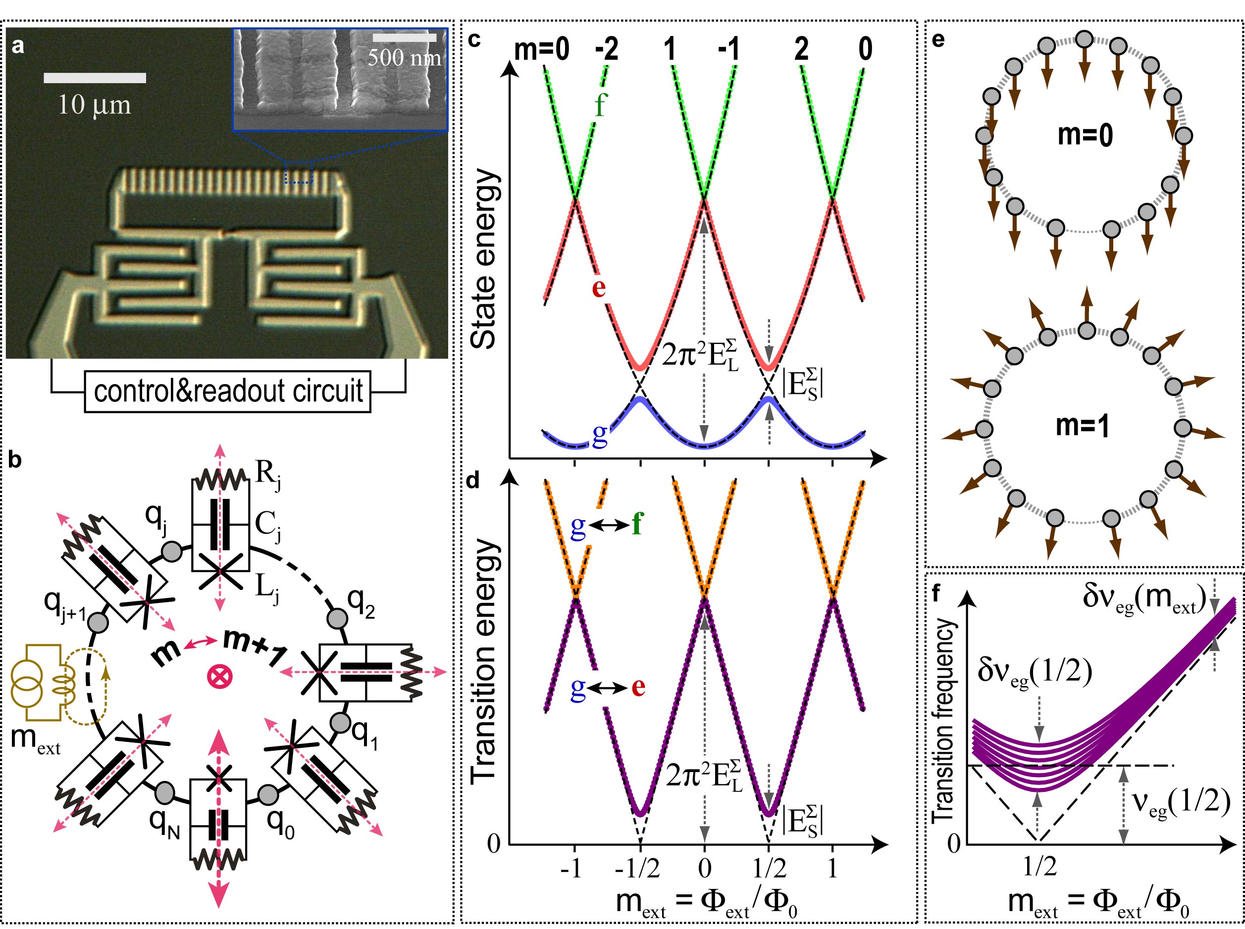
Figure 1: (a) Optical image of the fluxonium device, bright color for Al, dark color for Si substrate. Two finger capacitors couple the small junction of the loop to the dispersive microwave reflectometry setup. Inset: Scanning electron micrograph of an array section. (b) Effective electrical circuit of the device with minimal elements for quantum phase-slip description. Each junction consists of a non-linear Josephson inductance $L_{j}$, a capacitance $C_{j}$, and an effective frequency-dependent resistance $R_{j}$ representing possible intrinsic losses; every island carries offset charge $q_{j}$ induced by charged impurities in the oxide or unpaired quasiparticles. Pink arrows indicate possible semiclassical phase-slip trajectories. Charge-dependent energy shifts of artificial atom levels correspond to closed trajectories crossing several junctions (not represented on the figure). (c) Low-energy spectrum of the Josephson ring. Dashed parabolas represent energy of loop Josephson inductance threaded by an integer number $m$ of flux quanta and tuned with external flux $m_{\mathrm{ext}}$. (d) Two lowest transitions from the ground state. (e) Sketch of spatial distribution of superconducting phases of array islands, corresponding to the states with $m=0$ (no phase-slips) and $m=1$ (one phase-slip) across the entire loop at $m_{\mathrm{ext}}=0$. Phase of each island is represented by the angle between the corresponding arrow and the vertical. The value of $m$ coinsides with the total phase winding along the loop devided by $2\pi$. (f) Schematic broadening of the ground to first excited state transition $g\rightarrow e$ due to a spread of CQPS amplitude across the array. Origin of the spread is the combination of Aharonov-Casher effect and time-dependence of offset charges $q_{j}$ of array islands. Average transition frequency at $m_{\mathrm{ext}}=1/2$ is dominated by the phase-slip across the weak junction.

Fluxonium qubit (Fig. 1a, Fig. 5) may be viewed as one junction shunted by the kinetic inductance of a series array of $N\gg 1$ larger junctions Manucharyan2009 . Alternatively, we may view it as a loop of $N+1$ junctions connected in series, with one “black-sheep” weaker junction (Fig. 1b). The quantum state of the device is monitored by coupling the weak junction capacitively to an electromagnetic resonator, which provides a non-dissipative microwave readoutSchuster2005 ; Wallraff04 .

The loop array can first be understood qualitatively by the following semiclassical approach. Quantum fluctuations of the phase across a selected $j$-th Josephson junction are controlled by the ratio of its Josephson energy ($E_{J_{j}}=(\Phi_{0}/2\pi)^{2}/L_{j}$, $L_{j}$ being junction inductance) and charging energy ($E_{C_{j}}=e^{2}/2C_{j}$, $C_{j}$ being junction capacitance). We neglect the capacitances of the array islands to ground (any large size metal object in the vicinity of the device). This is made possible by a tight packing of array junctions (Fig. 1a-inset), as justified in our previous work Manucharyan2009 .

For large $E_{J_{j}}/E_{C_{j}}$, phase fluctuations are small. Correspondingly, quantum phase-slips crossing a ring made of such junctions occur rarely. This allows one to reduce the many-body Hamiltonian describing the quantum dynamics of phases in the ring to a simplified, low-energy Hamiltonian MLG2002 . In the basis of states labeled by the number $m$ of phase-slips which crossed the ring the Hamiltonian is given by (model A)

$$H =\frac{1}{2}E_{L}^{\Sigma}(2\pi)^{2}\sum\limits_{m}(m-m_{\mathrm{ext}})^{2}\left|m\right\rangle\left\langle m\right|$$

$$+\sum\limits_{m}\left[\frac{1}{2}E_{S}^{\Sigma}\left|m\right\rangle\left\langle m+1\right|+\mathrm{h.c.}\right]\,.$$ (1)

Here $E_{L}^{\Sigma}=\left(\Phi_{0}/2\pi\right)^{2}/L_{\Sigma}$ corresponds to the inductive energy of the current in the loop of total inductance $L_{\Sigma}=\sum L_{j}$; the hybridization matrix element $E_{S}^{\Sigma}$ is proportional to the CQPS probability amplitude in the loop, and we assume $|E_{S}^{\Sigma}|\ll$ $E_{L}^{\Sigma}$, so that one can neglect non-nearest-neighbor terms (like $m\leftrightarrow m+2$); an externally applied magnetic field offsets the total flux in the loop by an amount $\Phi_{\mathrm{ext}}=$ $m_{\mathrm{ext}}\Phi_{0}$.

In the absence of CQPS, i.e. $E_{S}^{\Sigma}=0$, the energy levels of the ring depend quadratically on $m_{\mathrm{ext}}$ for a given $m$ (Fig. 1c), and present two-fold degeneracy at half-integer $m_{\mathrm{ext}}$. The energy difference between the ground $g$ and first excited $e$ states varies in a zig-zag manner as a function of $m_{\mathrm{ext}}$. CQPS removes the degeneracy, which leads to the rounding of the zig-zag corners at half-integer $m_{\mathrm{ext}}$. Moreover, the presence of CQPS allows $e\leftrightarrow g$ coherent transitions under external radiation at any $m_{\mathrm{ext}}$.

Interestingly, the collective nature of the strongly-coupled junctions in this model hides in the specific form of the matrix element $E_{S}^{\Sigma}$. Namely,

$$E_{S}^{\Sigma}\{Q\}=\sum\limits_{j=0}^{N}E_{S_{j}}\mathrm{e}^{i2\pi Q_{j}/2e}\,,$$ (2)

where $E_{S_{j}}$ is the “microscopic” contribution of an individual quantum phase-slip along the $j$-th junctionESnote and $Q_{j}$ is the total charge on the islands between the $0$-th and $j$-th junction, i.e $Q_{j}=\sum\limits_{i=0}^{j}q_{i}$, with $q_{j}$ being the charge on $j$-th island (Fig. 1b). As long as $N\gg 1$, one can view each quantum phase-slip event as tunneling of a fictitious particle carrying flux $\Phi_{0}$ from the inside of the loop to the outside (and vice-versa). Tunneling occurs via a superposition of multiple paths crossing different junctions and therefore encircle island charges. Tunneling through each individual junction $j$ then contributes to the total CQPS amplitude Eq. (2) with the corresponding Aharonov-Casher geometric phase AC ; Elion ; AverinFriedman ; Ivanov ; MLG2002 $2\pi Q_{j}/2e$.

In real superconducting circuits, however, non-equilibrium charged impurities and quasiparticles cause the offset charges to fluctuate in time with an amplitude comparable to $e$, often on sub-$\mathrm{ms}$ time scales Aumentado2004 , much shorter than the averaging time of a typical qubit experiment. In the case of a homogeneous array $(E_{S_{i}}\simeq E_{S_{j}}$ $\forall i,j)$, fluctuations of $E_{S}^{\Sigma}$ and, as a result, fluctuations of the transition matrix element $\left\langle g|m|e\right\rangle$, which couples the qubit to the external radiation, are comparable to their respective means (see Appendix B.1). This makes slow spectroscopic measurement at $m_{\mathrm{ext}}=1/2$, and time-domain coherence measurements at any $m_{\mathrm{ext}}$ technically challenging. We circumvent this obstacle by introducing an inhomogeneity in the array in the form of one ($j=0$, for definiteness) weak “black-sheep” junction. Since the phase across the weaker junction fluctuates more strongly, the corresponding phase-slip amplitude $E_{S_{0}}$ at $j=0$ largely exceeds that for all other (array) junctions, $E_{S_{0}}\gg E_{SA}\equiv\overline{E_{S_{j\neq 0}}}$, where the averaging is taken over the junction index. Now, the Aharonov-Casher interference contrast is reduced from unity to a much smaller value of order $\sqrt{N/2}E_{SA}/E_{S_{0}}$, where the $\sqrt{N}$ factor comes from averaging over random charges. Effectively, we split the roles of phase-slips in different junctions: while phase-slips across the black-sheep mix states of the loop with different $m$ and therefore shape the qubit transition spectrum (Fig. 1b-c), the CQPS in the array junctions, combined with the fluctuating island charges, induce an inhomogeneous broadening $\delta\nu_{eg}$ to the qubit $g\leftrightarrow e$ transition. This linewidth is maximal at $|m_{\mathrm{ext}}|=1/2$, where it is given by $\delta\nu_{eg}(1/2)=\sqrt{N/2}E_{SA}/h$, and diminishes away from that spot according to the following expression

$$\delta\nu_{eg}(m_{\mathrm{ext}})=\delta\nu_{eg}(1/2)\frac{\nu_{eg}(1/2)}{\nu_{eg}(m_{\mathrm{ext}})}$$ (3)

(Fig. 1f). The factor $\sqrt{N/2}$ comes from averaging $|E_{S}^{\Sigma}|$ over the random charges, assuming $E_{S_{0}}\gg E_{SA}$.

CQPS thus remarkably turn the flux-noise sweet spot into charge noise anti-sweet spot. We have now arrived at the main idea behind our experiment: by measuring the variation of the dephasing time $T_{2}^{\ast}$ of the $g\leftrightarrow e$ transition of the fluxonium circuit as a function of external flux $m_{\mathrm{ext}}$, we resolve the effect of CQPS in the Josephson junction array, provided that the transition intrinsic linewidth is smaller than the characteristic frequency $\sqrt{N/2}E_{SA}/h$ of the CQPS. Evidence for CQPSs consists of: (i) the presence of the dephasing anti-sweet spot at $|m_{\mathrm{ext}}|=1/2$, (ii) excellent quantitative agreement of the observed dephasing time as a function of $m_{\mathrm{ext}}$ with the described below parameter-free prediction Eq. (6), and (iii) confirmation of the inhomogeneous nature of the dephasing in echo measurements. The latter also allow us to extract limits for the time scale of charge re-arrangements.

We introduce now a quantitative model of quantum phase-slips in the fluxonium circuit (model B). Unlike Eq. (1), now we need to allow strong phase fluctuations in one of the junctions, while phase-slips in all others are still rare. Therefore, we use a mixed representation: the black-sheep junction is described by a continuous fluctuating phase $\varphi$; the dynamics of the remaining array of large junctions is treated by the same tight-binding type model as Eq. (1) in the space of the number $\tilde{m}$ of CQPS across the array of large junctions only. The variables $\varphi$ and $\tilde{m}$ are coupled because phase-slips in the array of large junctions create a phase bias on the black sheep. Thus, the Hamiltonian of model B is

$$H =H_{F}(\varphi,~{}m_{\mathrm{ext}}-\tilde{m})$$

$$+\sum\limits_{\tilde{m}}\left[\frac{1}{2}E_{S}\left|\tilde{m}\right\rangle\left\langle\tilde{m}+1\right|+\mathrm{h.c.}\right]\,,$$ (4)

where

$$H_{F}(\varphi,m_{\mathrm{ext}}) =-4E_{C}\frac{\mathrm{\partial}^{2}}{\mathrm{\partial}\varphi^{2}}-E_{J}\cos\varphi$$

$$+\frac{1}{2}E_{L}(2\pi)^{2}(\varphi/2\pi-m_{\mathrm{ext}})^{2}\,,$$ (5)

$E_{J}=E_{J_{0}}$, and $E_{C}=E_{C_{0}}$. The CQPS amplitude $E_{S}\{Q\}=E_{S}^{\Sigma}\{Q\}-E_{S_{0}}$ is different from that in Eq. (2) and accounts for phase-slips through every junction except the black-sheep one (we have set $Q_{0}=0$ without the loss of generality). Similarly, the new inductive energy $E_{L}$ excludes the contribution of the black-sheep junction inductance from the total inductive energy of the loop; $1/E_{L}=$ $1/E_{L}^{\Sigma}-1/E_{J_{0}}$. For $E_{S}=0$, expressions (4) and (5) define the Hamiltonian of the fluxonium qubitManucharyan2009 . The second term in Eq (4) incorporates the CQPS in the fluxonium inductance, and $\tilde{m}$ now counts their number. We are now in a position to evaluate accurately the flux dependence of the Aharonov-Casher linewidth of any $\alpha\leftrightarrow\beta$ fluxonium transition. First order perturbation theory in $|E_{S}|$ results in a remarkably simple expression (see Appendix B.1 for details of derivation):

$$\delta\nu_{\alpha\beta}(m_{\mathrm{ext}})=\frac{E_{SA}\sqrt{N/2}}{h}\left|F_{\alpha\beta}(m_{\mathrm{ext}})\right|\,,$$ (6)

where

$$F_{\alpha\beta}(m_{\mathrm{ext}}) =\int\limits_{-\infty}^{\infty}\mathrm{d}\varphi\Psi_{\alpha}(\varphi)\Psi_{\alpha}(\varphi-2\pi)$$

$$-\int\limits_{-\infty}^{\infty}\mathrm{d}\varphi\Psi_{\beta}(\varphi)\Psi_{\beta}(\varphi-2\pi)$$ (7)

with $\Psi_{\alpha}(\varphi)$ being the eigenfunction of the $\alpha$-th energy state of the fluxonium Hamiltonian (5); it can be readily computed numerically.

The dependence of $\delta\nu_{\alpha\beta}$ on the external flux $m_{\mathrm{ext}}$ comes from the presence of $m_{\mathrm{ext}}$ in Eq. (5) determining the wave functions $\Psi_{\alpha,\beta}(\varphi)$ which enter Eq. (7). For small amplitude of CQPS and for $|m_{\mathrm{ext}}|$ close to $1/2$, one recovers the relation (3) from Eq. (6). The overlap function $F_{\alpha\beta}$ also appears in a previous workHriscuNazarov and can be understood from the fact that a phase-slip through the array inductance must shift the center of gravity of $\Psi_{\alpha}(\varphi)$ by $2\pi$. The external flux dependence of the Aharonov-Casher linewidth thus encodes the overlap of the $2\pi$-shifted fluxonium wave functions (Fig. 10). The flux dependence of the linewidth (6) of our model B generalizes Eq. (3) of the intuitive model A to the case of arbitrary black-sheep junction parameters.

Finally, since the finite lifetime of fluxonium excited states limit our experiment, and given the large number $N$ of array junctions, a natural question arises: does the dissipation in the array scale up with $N$? Every junction of the array suffers from intrinsic, generally unknown dissipation sources, all lumped into a frequency-dependent resistance $R_{j}$ shunting the $j$-the junction (Fig. 1b). Fortunately (and counterintuitively) the dissipation in the black-sheep junction solely dominates the intrinsic relaxation of the phase-slips spectrum with contribution from array junctions being suppressed as $1/N$. Indeed, the dominant phase-slip process generates a voltage pulse across the black-sheep; each array junction receives only a $1/N$ portion of that voltage, and the total energy dissipated in the array resistors is only $1/N$ of that dissipated in the black-sheep junction. We thus conclude that, remarkably, the apparent multi-junction complexity of the fluxonium circuit does not a priori penalize it with enhanced energy relaxation.

III Experiments

In this section we present measurements of the transition frequencies of a fluxonium qubit obtained using both frequency-domain and time-domain techniques, and analyze our data using the theory developed in section II. We read out the qubit state with the help of a microwave resonator, the technique known as circuit QED Schuster2005 ; Wallraff04 . Details of this technique are described in the Appendix, Sections A.2, A.3, and A.4. Capacitive coupling of the fluxonium circuit to the readout resonator results in the shift of the frequency of this resonator depending on the quantum state of fluxonium according to Eq. (12). Essentially, the qubit state is mapped onto a particular value of the shift of the resonance frequency of the readout resonator. This frequency shift is in turn detected by measuring the phase (Eq. (9)) of the reflection amplitude (Eq. (8)) for a microwave signal, scattered off the resonator.

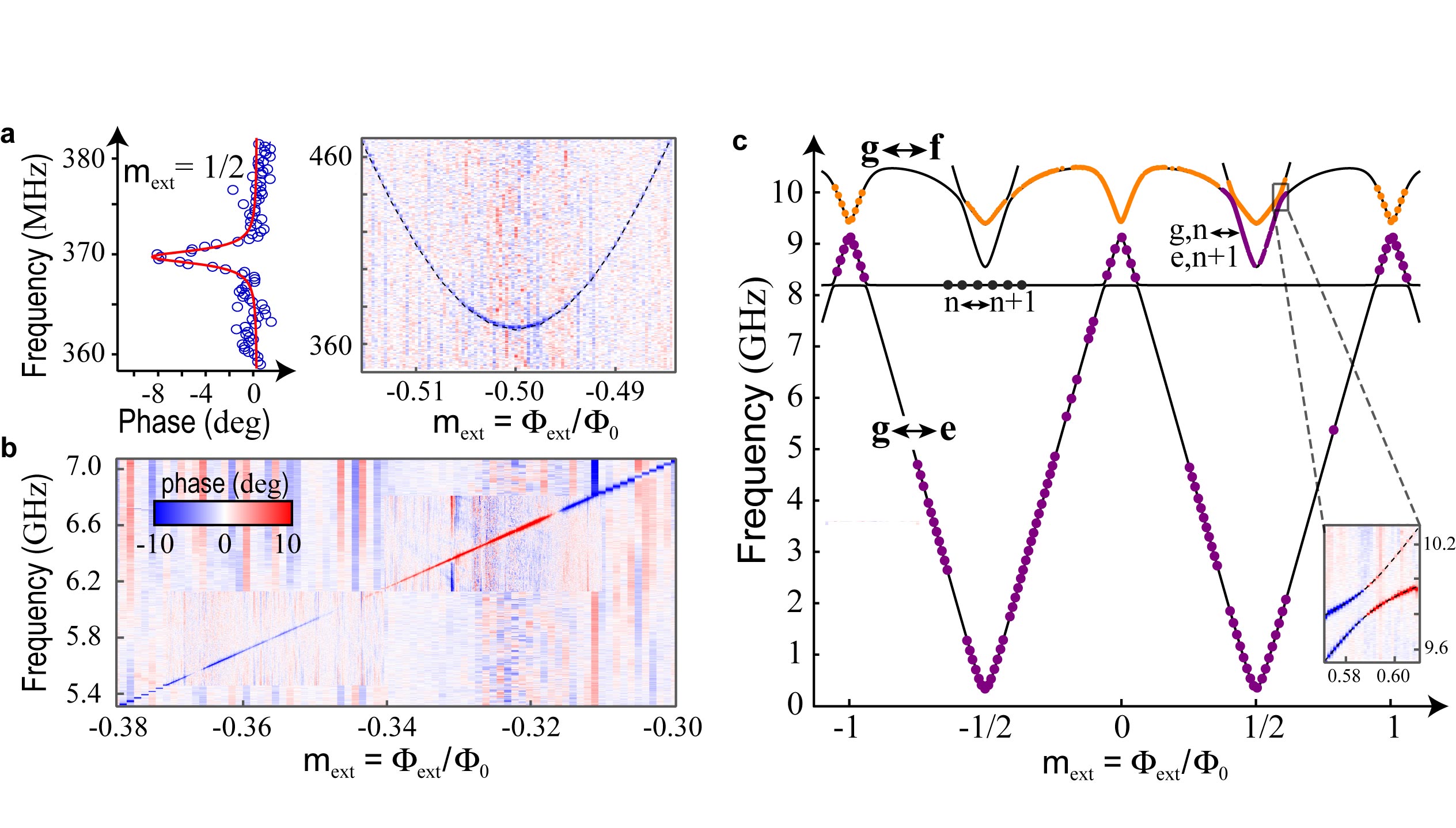
Figure 2: (a) Left: Transition between $g\leftrightarrow e$ fluxonium ground and first excited states at $|m_{\mathrm{ext}}|=1/2$ measured by sweeping spectroscopy (Y-axis) frequency and measuring phase response of the $8.2$ $\mathrm{GHz}$ microwave cavity coupled to the qubit (X-axis). Right: Raw spectroscopy data consisting of traces like that on the left but with Y color-coded, as a function of external flux, in the vicinity of $|m_{\mathrm{ext}}|=1/2$; (b) Large scale spectroscopy data as a function of flux and frequency. (c) Extracted resonance locations vs spectroscopy frequency and applied flux. Solid line represent the fit to numerically diagonalized Hamiltonian neglecting quantum phase-slips in the array but taking into account interaction with readout cavity mode. Horizontal line represents cavity mode. Inset shows strong, $160~{}\mathrm{MHz}$ anticrossing of the cavity-assisted blue sideband of the qubit lowest transition with the second lowest qubit transition, on which the readout mechanism is based.

Spectroscopy of fluxonium. Spectroscopy data in the range of qubit transition frequencies from $300~{}\mathrm{MHz}$ to $12$ $\mathrm{GHz}$ and for the full span of external flux bias reveals the spectrum of the transitions between the $3$ lowest energy levels (Fig. 2). The phase-slip frequency of the black-sheep junction, $\nu_{eg}(m_{\mathrm{ext}}=1/2)=|E_{S_{0}}|/h=369~{}\mathrm{MHz}$ corresponds to the center frequency of the line observed at $m_{\mathrm{ext}}=1/2$ (Fig. 2a-left). By varying $m_{\mathrm{ext}}$ around that point and plotting spectroscopy traces on a 2D color plot (Fig. 2a-right) we observe the anti-crossing of the states of the loop with the phase-slips number $m$ differing by a unity. Apart from the neighborhood of $m_{\mathrm{ext}}=1/2$ and $m_{\mathrm{ext}}=0$, the transition frequency depends linearly on the applied flux with a slope given by $E_{L}$, up to corrections of order $E_{L}/E_{J_{0}}\simeq 0.06$ (Fig. 2b). In $m_{\mathrm{ext}}-\nu$ plane (Fig. 2c), one recognizes the anticipated zig-zag shape (Fig. 1d) of the lowest $g\leftrightarrow e$ transition (Fig. 2c).

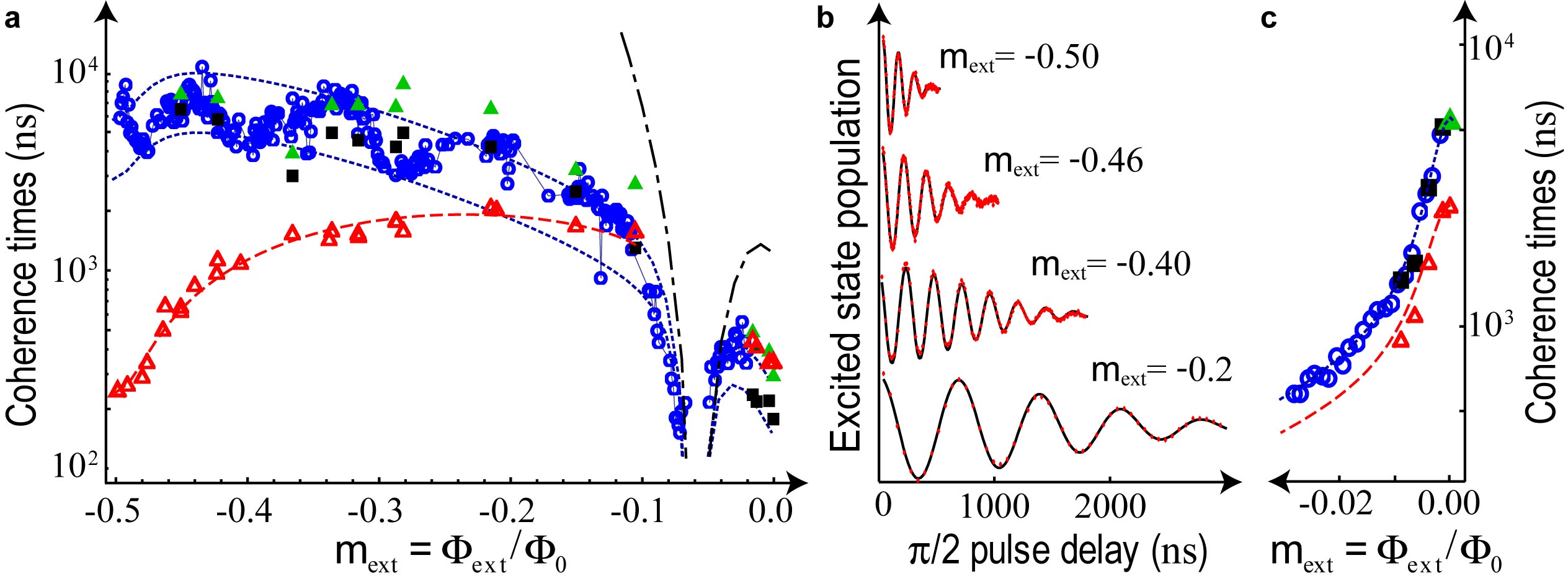
Figure 3: (a) Summary of the coherence times measurements of the $g\leftrightarrow e$ transition. Blue open circles denote energy decay times ($T_{1}$), red open triangles - decay time of the Ramsey fringes ($T_{2}^{\ast}$) and closed green triangles the decay of the $\pi$-pulse echo experiment ($T_{2}$). Black squares are the $T_{1}$ data measured simultaneously with the echo data. The dash-dotted line represent the calculated relaxation time into the readout cavity (Purcell effect), which clearly is irrelevant for the most of the data. The two dotted lines are theoretical predictions of relaxation, for the two absolute values of effective resistance discussed in the text. Relaxation times $T_{1}$’s present temporal variations that are not repeatable (differences between blue open and solid circles), while the overall dependence with applied flux is. Dashed line corresponds to the theory of the Aharonov-Casher effect induced dephasing, with the overlap function calculated numerically using circuit parameters extracted by spectroscopy. (b) Actual Ramsey fringes for several values of flux bias, with matched scale of the Y-axes for clarity. (c) Coherence time of the $g\leftrightarrow f$ transition. Notations match those of (a), except that all relaxation times were multiplied by 2 for easy comparison with dephasing times. Theory lines obtained using same parameters as those for $g\leftrightarrow e$ transition.

The anticrossing at $m_{\mathrm{ext}}=0$ between transitions $g\leftrightarrow f$ and $g\leftrightarrow e$ (Fig. 2c) is associated with the hybridization between states $m\leftrightarrow m+2$. The size of this anticrossing according to model A would be orders of magnitude smaller than $\nu_{eg}(m_{\mathrm{ext}}=1/2)$, the latter is associated with the hybridization $m\leftrightarrow m+1$. However, we find that the two frequencies are of the same order, because of the proximity of transitions $g\leftrightarrow f$ and $g\leftrightarrow e$ at $m_{\mathrm{ext}}=0$ to the plasma resonance in the black-sheep junction, which model B properly takes into account.

The $g\leftrightarrow f$ transition anticrosses the cavity-assisted blue sideband of the $g\leftrightarrow e$ transition, which appears as a copy of the $g\leftrightarrow e$ transition (Fig. 2c and inset). This anticrossing is an unusual vacuum Rabi resonance between the readout cavity and the $e\leftrightarrow f$ transition of the qubit, as indicated by the pole in the dispersive shift expression (12) at $\nu_{ef}=\nu_{0}$. The magnitude of this anticrossing (Fig. 2c-inset), which exceeds $100~{}\mathrm{MHz}$ demonstrates the strong coupling of the qubit to the readout and accounts for the good qubit visibility in the remarkable $5$-octave transition frequency range. The frequencies of all transitions are in perfect agreement with a numerical diagonalization of the hamiltonian of model B (neglecting $E_{S}$). This allows us to extract accurately the circuit parameters values from spectroscopy data, see Table (1).

Measurement of decoherence times of fluxonium. We now turn to the time-domain experiments. The coherence of the $g\leftrightarrow e$ transition (Fig. 2a) is analyzed using standard time domain techniques in the full range of flux and frequency $(-0.5\leqslant m_{\mathrm{ext}}\leqslant 0$;$~{}0.369~{}\mathrm{GHz}\leqslant\nu_{eg}\leqslant 9.1~{}\mathrm{GHz})$. First, the contribution of the energy relaxation, is measured by the standard $\pi$-pulse techniques and yields the exponential decay times $T_{1}$ of the excited state. Theoretical expression for $T_{1}$ is given by Eqs. (18), (19), (20), and (21). In the narrow $300~{}\mathrm{MHz}$ vicinity of the cavity frequency, $T_{1}$ is limited by relaxation into the cavity (Purcell effect). Subtracting that effect, the overall shape of the $T_{1}(m_{\mathrm{ext}})$ data is matched well (within a factor of $2)$, by dissipation across the black-sheep junction through effective shunting resistance of the form $R_{0}(\omega)=A/\omega$. Note that this agreement takes place for $T_{1}$ varying by two order of magnitude and over a $4-$octave frequency span. The only adjustable parameter is the value of $A=190\pm 60$ $\mathrm{M\Omega}\times\mathrm{GHz}$, the extreme values corresponding to top and bottom dashed lines (Fig. 3a). Such $1/\omega$ frequency dependent resistance usually arises from the coupling to a large ensemble of discrete energy absorbersMartinis , whose microscopic origin is presently unclear FaoroIoffe . Dissipation across the black-sheep may likely come from dielectric losses in the coupling finger capacitors (Fig. 1a). Alternatively, our energy relaxation data could be explained by a lossless black-sheep and dissipation in the larger area junctions of the array, but with the $A$ factor $N=43$ stronger.

Dephasing times $T_{2}^{\ast}$ of the $g\leftrightarrow e$ transition, measured from the decay of Ramsey fringes, display pronounced minimum of about $250$ $\mathrm{ns}$ at the flux sweet-spot and spectacularly rise by almost an order of magnitude (Fig. 3a-b), exceeding $2$ $\mathrm{\mu s}$ at $|m_{\mathrm{ext}}|\simeq 0.2$ ($\nu_{ge}=$ $5.5$ $\mathrm{GHz}$). Around $|m_{\mathrm{ext}}|=1/2$, the decay of Ramsey fringes is well fitted (Fig. 3b) with a gaussian. This confirms the irrelevance of the energy relaxation for $|m_{\mathrm{ext}}|>0.2$, while it dominates at $m_{\mathrm{ext}}$ close to zero. Coherence times $T_{2}$ obtained with echo experiments are drastically larger than $T_{2}^{\ast}$, particularly around $|m_{\mathrm{ext}}|=1/2$, and, for the most part, turn out to be limited by energy relaxation, i. e. $T_{2}\approx 2T_{1}$ (Fig. 3a). Therefore, the noise that causes Ramsey fringes to decay is slow on the time scale of order $T_{2}$ (about $10~{}\mathrm{\mu}$s) but fast on the time scale of the typical Ramsey fringe acquisition time, of order one minute, typical of $e$-jump rates seen with superconducting single electron transistors and charge qubits Aumentado2004 ; Houck .

Experimental evidence for the CQPS. Analyzing our time-domain data, we find that the measured flux dependence of the decoherence times $T_{2}^{\ast}(m_{\mathrm{ext}})$ of the $g\leftrightarrow e$ transition is in excellent agreement with the expressions (6) and (7). Moreover, our data is inconsistent with conventional decoherence mechanisms, which include low-frequency noise in the flux $m_{\mathrm{ext}}$, the Josephson energy $E_{J}$ (due to critical current noise of the black-sheep junction), and in the inductive energy $E_{L}$ (due to critical current noise in array junctions).

For the flux-noise mechanism, according to Eq. (23) and Fig. 2, we expect $T_{2}^{\ast}(m_{\mathrm{ext}})$ to be maximal at $|m_{\mathrm{ext}}|=1/2$ (flux sweet-spot). This is obviously inconsistent with our data, which shows a clear minimum of $T_{2}^{\ast}(m_{\mathrm{ext}})$ at $|m_{\mathrm{ext}}|=1/2$, see Fig. 3a. Dephasing due to fluctuations in the array inductance, given by Eq. (25), is also ruled out because the corresponding $T_{2}^{\ast}(m_{\mathrm{ext}})$ would also peak at $|m_{\mathrm{ext}}|=1/2$. (Qualitaively, this is because at $|m_{\mathrm{ext}}|=1/2$ the transition frequency $\nu_{eg}$ is given by $|E_{S}^{\Sigma}|/h$, which is a property of the black-sheep junction, and is independent of the array inductance ESnote .) The numerically evaluated sensitivity of the transition frequency $\nu_{eg}$ to $E_{L}$ is presented in Fig. 13b. Theoretical analysis of the sensitivity of $\nu_{eg}$ to the critical current noise in the black-sheep junction (Eq. (24), Fig. 13a) shows that the sensitivity must turn zero at some device-specific flux bias. Such non-monotonic dependence is inconsistent with the observed monotonic $T_{2}^{\ast}(m_{\mathrm{ext}})$.

Our key result is that the highly unusual flux-dependence of the dephasing time $T_{2}^{\ast}(m_{\mathrm{ext}})$ (Fig. 3a) is well explained with the Aharonov-Casher effect of phase-slip interference. Upon adding the measured small contribution $1/2T_{1}$ to the expression (17) obtained from our theory of CQPS-induced dephasing, see Eqs. (4)-(7) and Appendix B.1, we find excellent agreement with the data (Fig. 3a). The only adjustable parameter we use is the theoretical value of $T_{2}^{\ast}$ at $|m_{\mathrm{ext}}|=1/2$. Furthermore, this adjustable parameter agrees well with a WKB calculation of $E_{SA}\approx h\times 150$ kHz based on our estimates of the array junction parameters.

Control experiments. To verify our interpretation of the dephasing data in terms of the CQPS-induced broadening, we performed two main control experiments.

In the first control experiment, we check if phase-slips interference can explain the dephasing of some other fluxonium transition. For such experiment it is necessary to select a transition other than the lowest $g\leftrightarrow e$, but with sufficiently long $T_{1}$, so that the decoherence is dominated by dephasing and not by energy relaxation. A good candidate for this control experiment turns out the transition to the second excited state $g\leftrightarrow f$ in a narrow vicinity of $m_{\mathrm{ext}}=0$ (Fig. 2c). Interestingly, for this transition the flux bias $m_{\mathrm{ext}}=0$ turns out to be a sweet-spot for $T_{1}$, see Fig. 3c. The sharp increase of $T_{1}$ of the $g\leftrightarrow f$ transition at $m_{\mathrm{ext}}=0$ is well explained, see Eq. (22), by exactly the same model of dissipation, $R_{0}(\omega)=A/\omega$, used to explain energy relaxation of the $g\leftrightarrow e$ transition, with $A=190~{}M\Omega\times\mathrm{GHz}$. The origin of the peak in $T_{1}$ at $m_{\mathrm{ext}}=0$ comes from the fact that the $f$ state can decay either directly to $g$ or first to $e$ and then to $g$; at $m_{\mathrm{ext}}=0$, due to parity conservation, the direct $f\rightarrow g$ decay is forbidden Manucharyan2009 . Thus, the bottleneck at $m_{\mathrm{ext}}=0$ is a $280~{}\mathrm{MHz}$ $f\leftrightarrow e$ transition resulting in the lifetimes of the $g\leftrightarrow f$ transition of up to $3~{}\mu s$.

The Ramsey fringe measurement on the $g\leftrightarrow f$ transition at $m_{\mathrm{ext}}=0$, yields $T_{2}^{\ast}\simeq 2.5$ $\mu s$, a significantly smaller value than $2T_{1}\simeq 6~{}\mu s$. Echo measurement at $m_{\mathrm{ext}}=0$ yields a value of $T_{2}$ almost matching $2T_{1}$, see Fig. 3c. Thus, there is a noticeable amount of inhomogeneous broadening of the $g\leftrightarrow f$ transition at $m_{\mathrm{ext}}=0$. We find that this broadening is indeed precisely accounted for by expressions (6), (7), and (17). In other words, the ratio of $T_{2}^{\ast}=250$ ns of the $g\leftrightarrow e$ transition at $|m_{\mathrm{ext}}|=1/2$ and $T_{2}^{\ast}=2.5$ $\mu$s of the $g\leftrightarrow f$ transition at $m_{\mathrm{ext}}=0$ coincides with the theoretical prediction $F_{gf}(0)/F_{ge}(1/2)$, where the overlap integrals are computed without any adjustable parameters. The reduction of $T_{2}^{\ast}$ with the departure from the sweet-spot $m_{\mathrm{ext}}=0$ is also correctly reproduced without adjustable parameters (Fig. 3c).

The second control experiment is even more telling, and is performed on another fluxonium device, according to the following logic. Our theory of dephasing by the interfereing quantum phase-slips predicts that increasing the Josephson energy $E_{J_{j\neq 0}}$ of the array junctions while leaving their charging energy $E_{C_{j\neq 0}}$ the same, would suppress exponentiallyESnote the phase-slip matrix element $E_{SA}$. (Let us remind that we assume all the junctions of the fluxonium array to be nearly identical, i.e. $E_{J_{i}}\simeq E_{J_{j}}$ and $E_{C_{i}}\simeq E_{J_{j}}$ for any $i,~{}j>0$, so that $|E_{S_{i}}|\simeq|E_{S_{j}}|=E_{SA}$.) Thus, we shall be able to practically switch off the decoherence of fluxoium transitions due to CQPS in its array inductance, by a small adjustment of the array junctions parameters.

Parameters of the fluxonium device for the second control experiment were extracted from spectroscopy data (not shown) to be $E_{J_{j=0}}\equiv E_{J}=12.0~{}\mathrm{GHz}$, $E_{C_{j=0}}\equiv E_{C}=2.46~{}\mathrm{GHz}$, $E_{L}=0.89~{}\mathrm{GHz}$, very similar to the parameters of the main device (see Table 1). Since we kept the geometry of the array junctions and their number identical to the previous device, we infer that the charging energy of the array junctions $E_{C_{j\neq 0}}$ did not change significantly, while the Josephson energy $E_{J_{j\neq 0}}=N\times E_{L}=43\times 0.89=38~{}\mathrm{GHz}$ increased by a factor of $1.7$. For such device parameters, the spectrum of this fluxonium is similar to that of the main one. However, in sharp contrast to the main device, we find that $T_{2}^{\ast}(m_{\mathrm{ext}})$ for the $g\leftrightarrow e$ transition is now sharply peaked at $|m_{\mathrm{ext}}|=1/2$ and is nearly independent on $m_{\mathrm{ext}}$ away from this spot (Fig. 4). The reduction of $T_{2}^{\ast}$ away from the sweet-spot follows the prediction of the first-order flux-noise effect, Eq. (23), assuming the flux noise amplitude $\delta m_{\mathrm{ext}}\approx 10^{-5}$. The dependence $T_{2}^{\ast}(m_{\mathrm{ext}})$ away from the spot $|m_{\mathrm{ext}}|=1/2$ is now clearly inconsistent with the CQPS. (They still may be responsible for the dephasing at $|m_{\mathrm{ext}}|=1/2$.) The measured value of $T_{2}^{\ast}=4~{}\mathrm{\mu s}$ exactly at $|m_{\mathrm{ext}}|=1/2$ is too small to be explained by the second order flux-noise, but matches, within the factor of two, the prediction of Eq. (6) for the CQPS-induced dephasing. Thus, a second fluxonium device with nearly similar parameters, apart from an increase in $E_{J_{j\neq 0}}$ by a factor of $1.7$ resulted in a $16$-fold enhancement of the coherence time at $|m_{\mathrm{ext}}|=1/2$, indicating the expectedESnote exponential suppression of the phase-slip interference.

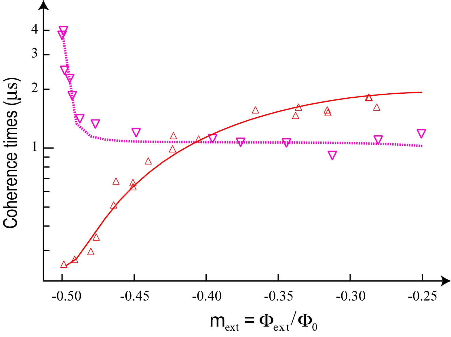
Figure 4: Measurement of the dephasing times $T_{2}^{\ast}$ of a new fluxonium device with supressed CQPS rate (magenta inverted triangles) and theoretical prediction (magenta dotted line). Data from Fig. 3a of the main text (red triangles) on $T_{2}^{\ast}$ of the main device is shown for easy comparison.For $|m_{\mathrm{ext}}|<0.25$, energy relaxation dominates the decoherence.

IV Summary

Coherent quantum phase-slips hybridize states of a superconductor with different configurations of the order parameter. The corresponding hybridization energy is exponentially small for “good” superconductors. In our experiment this energy, $|E_{S}|$, corresponds to only a few hundred $\mathrm{kHz}$, three orders of magnitude lower than the $15~{}\mathrm{mK}$ sample temperature, and five orders of magnitude lower than the main qubit energy scales, i. g. plasma frequency and the inductive energy (both of order $10~{}\mathrm{GHz}$). Detection of the tiny energy scale $|E_{S}|$ has been made possible by two ingredients specific to our experiment. First, the Aharonov-Casher modulation of CQPS amplitude broadens the qubit transitions. Second, the the immunity of the fluxonium circuit to dissipation ($Q=\nu_{eg}T_{1}\gtrsim 10^{5}$) allows us the high-precision measurement of this broadening, thus revealing CQPS. By replacing the junction array of the present experiment with an amorphous superconducting nanowire, but keeping the black-sheep junction, one may attempt seeing CQPS in nominally continuous wires with poorly controlled CQPS amplitudes.

Our experiment also shows that the fluxonium artificial atom may find applications in various quantum information processing schemes: it provides a 3-level system displaying a combination of larger frequency range and anharmonicity than most other qubits; it can operate away from flux sweet spots without loosing too much coherence; its coupling to a microwave cavity can be varied from weak to strong for exchange of quantum information without the side effect of spontaneous emission. In the event that critical current noise would end up dominating superconducting qubit coherence, one may expect a $1/\sqrt{N}$ suppression of this effect using an $N$ junction array. Finally, demonstrated coherence quality factor $Q$ exceeding $10^{5}$ in a circuit containing as many as $44$ junctions encourages the design of large quantum Josephson networks, especially those offering topologically protected ground states.

Appendix A Experimental techniques

A.1 Sample description

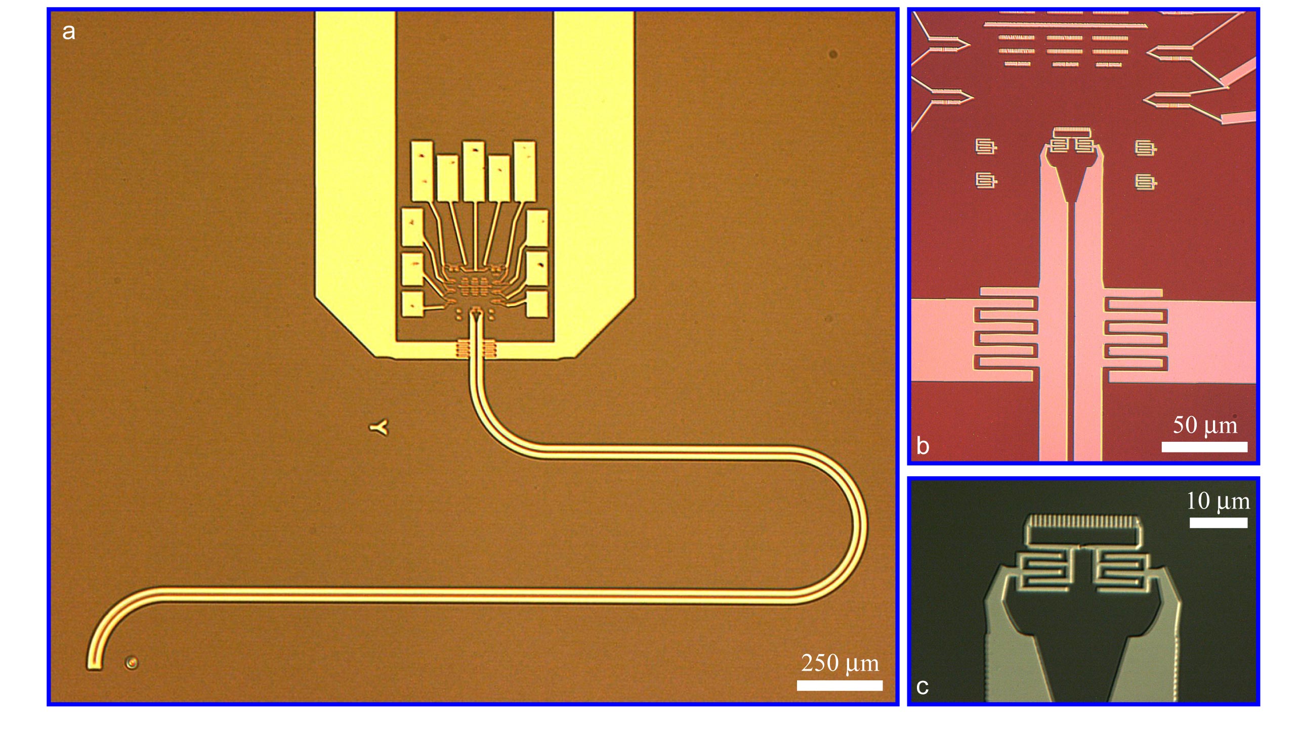
Figure 5: (a) Optical image of the sample (color filters applied for better contrast), bright indicates Al, dark indicates Si substrate. Sample contains the CPS resonator, the qubit, measurement leads and test structures. (b) Zoom in on the voltage antinode region of the resonator. (c) Further zoom on the fluxonium qubit loop.

The qubit and the readout circuits (Fig. 5a) are fabricated on a Si chip using Al double-angle evaporation through a suspended electron beam resist mask. The readout part consists of a resonator, implemented with a $\lambda/4$ coplanar-strips (CPS) transmission line. Resonator is coupled to $50~{}\Omega$ measurement leads (microstrips) using a pair of interdigitated capacitors (Fig. 5b). The two leads of the “black-sheep” junction are connected to the resonator strips with another pair of smaller interdigitated capacitors (Fig. 5c). A number of resistance and dose test structures are placed outside the resonator.

The fabrication procedure is outlined in the previous work Manucharyan2009 , with relevant device parameters collected into Table (1). We emphasize that the entire fluxonium device – including the Josephson array, the black-sheep junction, the resonator, and the test structures – is fabricated in a single step of e-beam lithography and double-angle evaporation. Such simplification in the fabrication of a superconducting qubit has been made possible because: i) the dimensions of both the black-sheep junction and the array junctions are chosen to be sufficiently close for patterning both types of junction in a single resist mask ii) the strips of the CPS resonator are sufficiently narrow so that the e-beam and lift off process used for the small junction fabrication could be readily applied to the resonator; in addition, space remains to accommodate test junctions and arrays fabricated simultaneously with the qubit.

Readout resonator strips width (measured)	$15~{}\mathrm{\mu m}$
Readout resonator strips separation (measured)	$4~{}\mathrm{\mu m}$
Readout resonator wave impedance $Z_{\infty}$ (inferred)	$80~{}\Omega$
Readout resonator resonance frequency $\nu_{0}$ (fit)	$8.175~{}\mathrm{GHz}$
Readout resonator external quality factor $Q_{\mathrm{ext}}$ (measured)	$400$
Readout resonator internal quality factor $Q_{\mathrm{int}}$ (measured)	$2000-5000$
Black-sheep junction dimensions (nominal)	$0.35~{}\mathrm{\mu m\times}0.2~{}\mathrm{\mu m}$
Array junction dimensions (nominal)	$2~{}\mathrm{\mu m\times}0.2~{}\mathrm{\mu m}$
Array inductive energy $E_{L}=(\hbar/2e)^{2}/L$ (fit)	$0.525~{}\mathrm{GHz}$
Array inductance $L$ (inferred)	$300~{}\mathrm{nH}$
Black-sheep junction Josephson energy $E_{J_{j=0}}\equiv E_{J}$ (fit)	$8.9~{}\mathrm{GHz}$
Black-sheep junction Coulomb energy $E_{C_{j=0}}\equiv E_{C}=e^{2}/2C_{J}$ (fit)	$2.5~{}\mathrm{GHz}$
Number of array junctions $N$ (nominal)	$43$
Array junction Josephson energy $E_{j\neq 0}=NE_{L}$ (inferred)	$22.5~{}\mathrm{GHz}$
Array junction Coulomb energy $E_{C_{j\neq 0}}$ (inferred)	$0.85-1~{}\mathrm{GHz}$
Qubit-cavity coupling constant $g$ (fit)	$181~{}\mathrm{MHz}$
Qubit-cavity coupling capacitance $C_{c}$ (inferred from $g$ and $Z_{\infty}$)	$0.8~{}\mathrm{fF}$
Black-sheep junction phase-slip energy $|E_{SB}|$ (measured, inferred)	$369~{}\mathrm{MHz}$
Array junction phase-slip energy $E_{SA}$ (inferred from $L$, $E_{J_{j\neq 0}}$, $E_{C_{j\neq 0}}$)	$50-250~{}\mathrm{kHz}$
Array junction phase-slip energy $E_{SA}$ (inferred from $T_{2}^{\ast}(m_{\mathrm{ext}}=1/2)$)	$130~{}\mathrm{kHz}$

Table 1: Device parameters

A.2 Microwave reflectometry readout

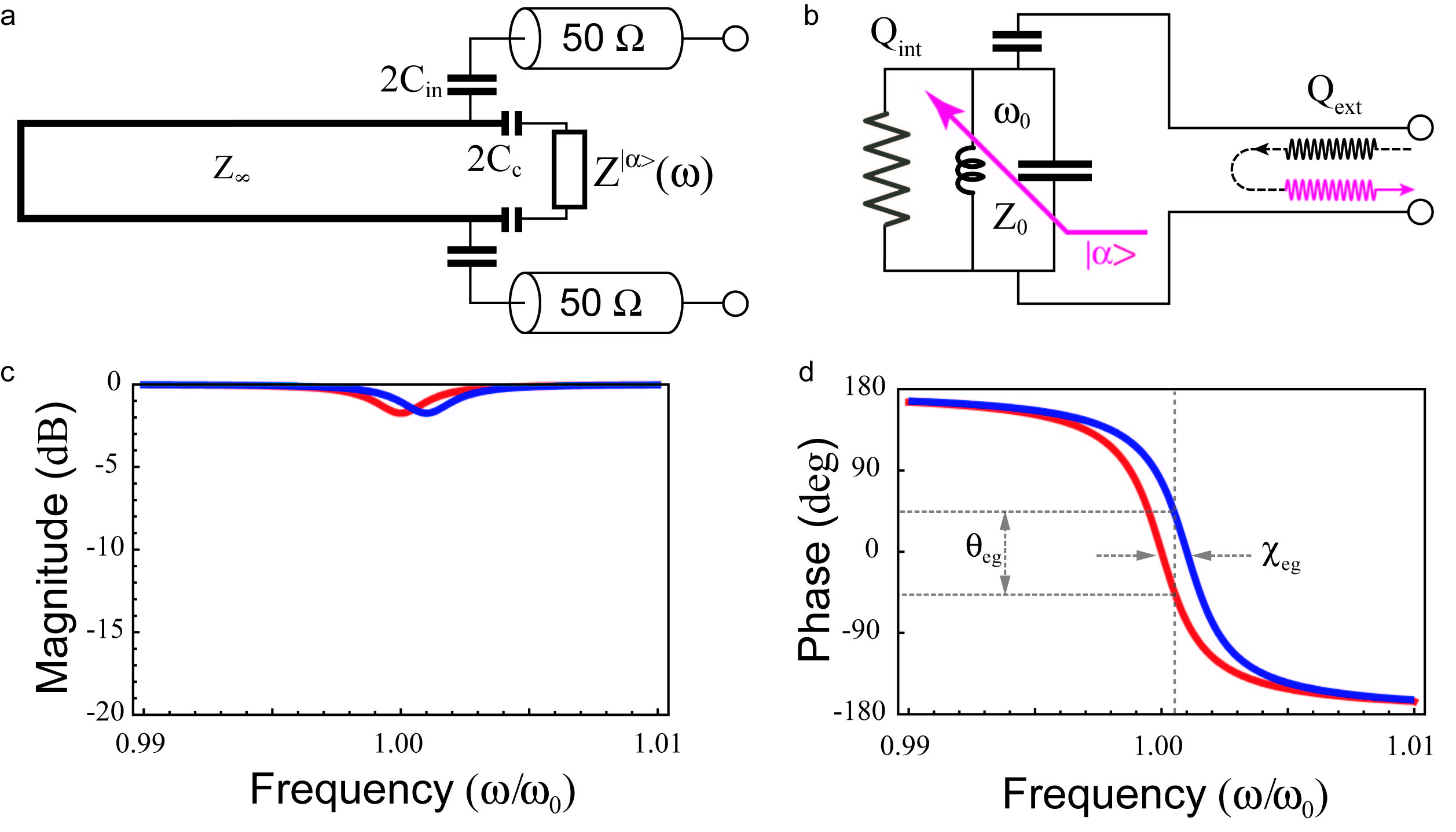
Figure 6: (a) Electrical model of a qubit interacting with the CPS transmission line resonator. Thick solid line represents the distributed transmission line. (b) Simplified circuit model of the dispersive effect of qubit on resonator. (c) Modulus of the reflection amplitude in model of panel (b) vs. signal frequency for $Q_{\mathrm{int}}=10Q_{\mathrm{ext}}$. Blue and red traces correspond to qubit states $g$ and $e$ respectively. (d) Phase of the reflection amplitude, same conditions as in panel (c).

We use the lowest differential mode of our resonator, which corresponds to the frequency $\omega_{0}$ at which the physical length of the CPS transmission line matches a quarter of the wavelength. The next order resonance lies at $3\omega_{0}$. The qubit can be viewed as a high impedance termination $Z^{\left|\alpha\right\rangle}(\omega)$ placed at the open end of the transmission line, and depends both on the frequency $\omega$ and the qubit state $\alpha$ (Fig. 6a). It provides a small contribution $\chi_{\alpha}$ - termed the dispersive shift - to the resonance frequency $\omega_{0}$, when the qubit is in state $\left|\alpha\right\rangle$. The shift in the resonance frequency is detected by monitoring the complex-valued reflection amplitude $\Gamma$ for the scattering of a microwave signal off the resonator. Approximating the single-mode resonance with an effective $LC$-oscillator (Fig. 6b), the reflection amplitude is given by

$$\Gamma(\omega,\omega_{0})=\frac{2i(\frac{\omega-\omega_{0}}{\omega_{0}})-Q_{\mathrm{ext}}^{-1}+Q_{\mathrm{int}}^{-1}}{2i(\frac{\omega-\omega_{0}}{\omega_{0}})+Q_{\mathrm{ext}}^{-1}+Q_{\mathrm{int}}^{-1}}~{},$$ (8)

where $Q_{\mathrm{ext}}$ is the quality factor due to the energy loss in the matched $50~{}\Omega$ measurement leads while $Q_{\mathrm{int}}$ is the quality factor due to the energy loss inside the resonator (electrically represented by a resistor shunting the $LC$-circuit). In our CPS resonator $Q_{\mathrm{ext}}\simeq 400\ll Q_{\mathrm{int}}\approx 4000$ making $|\Gamma(\omega,\omega_{0})|$ to be very close to unity (Fig. 6c). The phase $\theta=\mathrm{Arg}(\Gamma)$ of the reflected signal is a rapid function of frequency: $\theta=2\arctan 2Q_{\mathrm{ext}}\frac{\omega-\omega_{0}}{\omega_{0}}$ (Fig. 6d). Finally, the difference in phase of the reflection coefficient $\theta_{eg}=\theta_{e}-\theta_{g}$ between the qubit excited state $e$ and the ground state $g$ is given by

$$\theta_{eg}=2\arctan\left(2Q_{\mathrm{ext}}\frac{\chi_{g}}{\nu_{0}}\right)-2\arctan\left(2Q_{\mathrm{ext}}\frac{\chi_{e}}{\nu_{0}}\right)~{},$$ (9)

where $\nu_{0}=\omega_{0}/2\pi$ is the resonator frequency in $\mathrm{Hz}$. The quantity $\theta_{eg}$ is plotted on the Y-axes of Fig. 2a-left, and plotted as the color scale in Fig. 2a-right and in Fig. 2c.

Note that since $\theta_{eg}$ saturates quickly once $2Q_{\mathrm{ext}}\frac{\chi_{e}-\chi g}{\omega_{0}}>1$, increasing $Q_{\mathrm{ext}}$ above the value $\omega_{0}/|\chi_{e}-\chi_{g}|$ will not improve the sensitivity. In our experiment $|\chi_{e,f}-\chi_{g}|$ lie between $1~{}\mathrm{MHz}$ and $10~{}\mathrm{MHz}$, while $\nu_{0}=8.175~{}\mathrm{GHz}$, so $Q_{\mathrm{ext}}=400$ is a convenient choice with a measurement bandwidth of $20~{}\mathrm{MHz}$. We discuss the origin of the dispersive shifts as well as the effect of finite $Q_{\mathrm{ext}}$ on the qubit lifetimes (Purcell effect) in the text below, see Eqs. (18), (19), and (20).

A.3 Measurement schematic

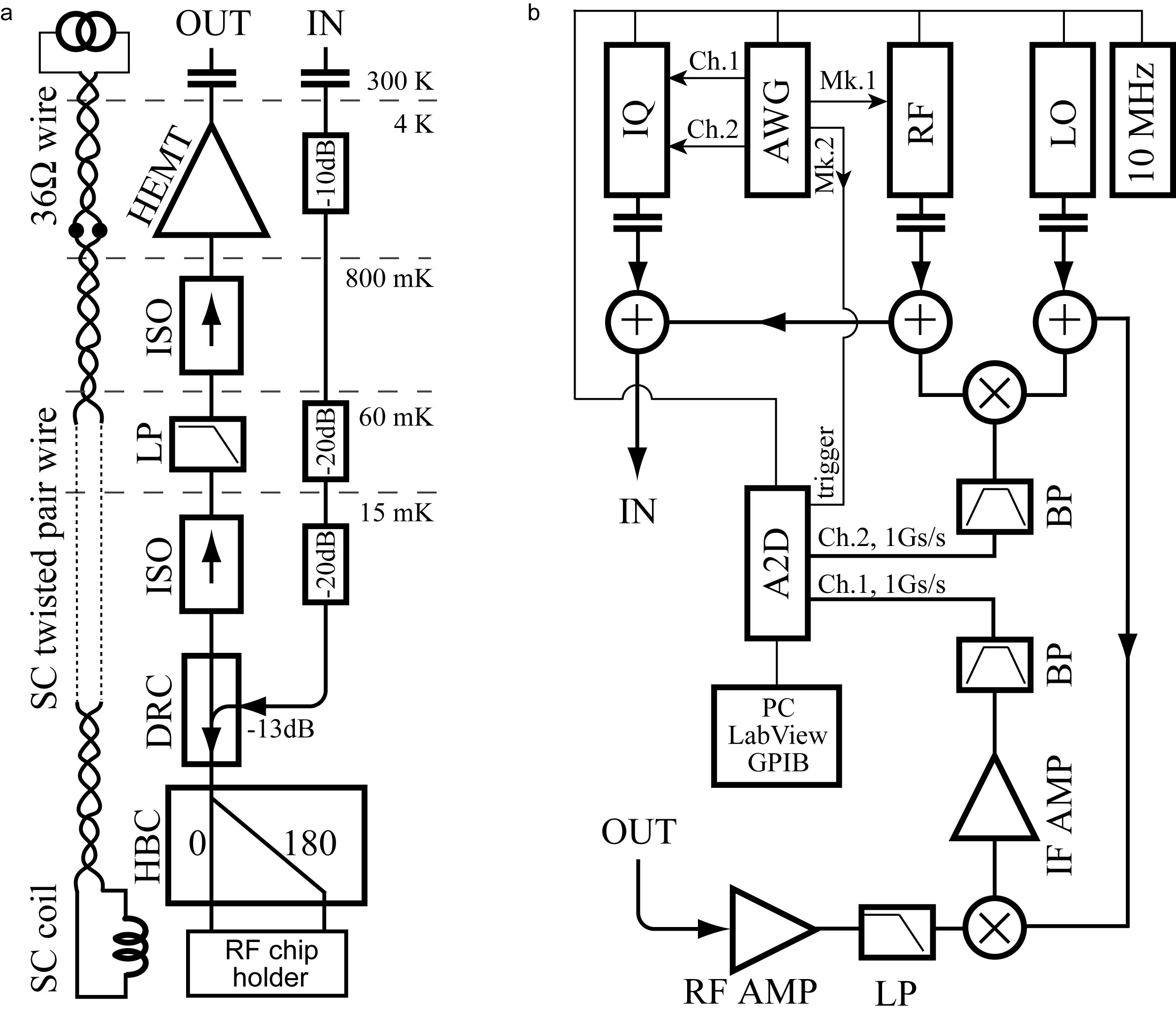
Figure 7: (a) Dilution refridgerator part of the microwave reflectometry setup. HEMT - high electron mobility cryogenic amplifier, ISO - cryogenic broadband isolator, LP - low pass filter, DRC - directional coupler, HBC - 180 degree hybrid coupler, see text for more details (b) Room-temperature signal generation and demodulation setup. LO - continuous microwave source, RF - pulsed (Mk.1 controlled) wave source, IQ is a vector signal generator for driving the qubit transitions, AWG - arbitrary waveform generator, A2D- two-channel fast digitizer, “$+$” - matched signal combiner/splitter, “$\times$” - microwave mixer, BP- and pass filter, “$10~{}\mathrm{MHz}$” - Rb reference, RF AMP - a room temperature microwave amplifier.

Low-temperature setup (Fig. 7a). The incoming signals line is attenuated with cryogenic high-frequency resistive film attenuators (XMA), with total attenuation exceeding $50~{}\mathrm{dB}$. The readout line is shielded by the two $4-12~{}\mathrm{GHz}$ isolators (Pamtech) and a low-pass filter (K&L) with rejection band $10-40~{}\mathrm{GHz}$. Outgoing signals are amplified using a $5~{}\mathrm{K}$ noise temperature cryogenic HEMT amplifier (Caltech). Incoming and outgoing waves are separated from each other using a directional coupler (Krytar). Differential excitation of the resonator is implemented using a $180$ degree hybrid coupler (Krytar). The chip rests at the bottom of the fully enclosing copper sample holder, the microwaves are guided to it by means of two printed circuit board microstrips wirebonded to their on-chip continuation, and perpendicular coaxial-to-microstrip transition implemented using Anritsu K connectors (Fig. 8). The transition provides less than $15~{}\mathrm{dB}$ return loss up to $20~{}\mathrm{GHz}$. Flux bias is provided by driving a hand-made superconducting coil (glued to the sample holder) with DC currents of order $1-10~{}\mathrm{mA}$.

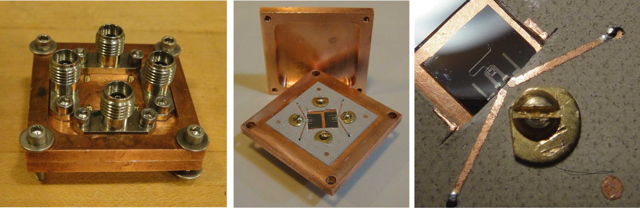
Figure 8: Photographs of the chip holder carrying the actual fluxonium device. Anritsu K connector guides microwaves from coaxial cables to Cu microstrip lines ($300~{}\mathrm{\mu m}$ wide) on the printed circuit board. The center conductor of the K connector is soldered to the begining of the microstrip. Microstrip lines continue to the chip by means of 5-6 short wirebonds.

Room-temperature setup (Fig. 7b). The readout signal is provided with Agilent E8257D generator (RF), the qubit pulses are generated using Agilent E8267D vector signal generator (IQ) combined with Tektronix 520 arbitrary waveform generator (AWG). Both readout and qubit signals are combined at room temperature and sent into the IN line of the refrigerator. The reflected $\sim 8~{}\mathrm{GHz~{}}$readout signal from the refrigerator OUT line is amplified at room temperature with a Miteq amplifier ($1-12~{}\mathrm{GHz}$, $30~{}\mathrm{dB}$ gain), mixed down with a local oscillator signal (LO), provided by HP 8672A, to a $50~{}\mathrm{MHz}$ IF signal, then filtered and amplified with the IF amplifier (SRS SR445A), and finally digitized using one channel of the $1~{}\mathrm{GS}/\mathrm{s}$ Agilent Acqiris digitizer. A reference IF signal is created by mixing a copy of RF and LO and digitized using the second channel. A software procedure then subtracts the phases of the two IF signals, resulting in a good long-term stability of the phase measurement. The short-term stability is implemented by phase locking every instrument to a Rb $10~{}\mathrm{MHz}$ reference (SRS FS725). The marker signals of the AWG are used as triggers to other instruments. Typical time to acquire Ramsey fringes of $5~{}\mathrm{\mu s}$ long (Fig. 3b) ranges from $10$ seconds to $1$ minute, without noticeable change in the fringe decay time. The magnetic coil is biased with Yokogawa 7751 voltage source in series with a $1:10$ voltage divider and a $1~{}\mathrm{k\Omega}$ resistor at room temperature.

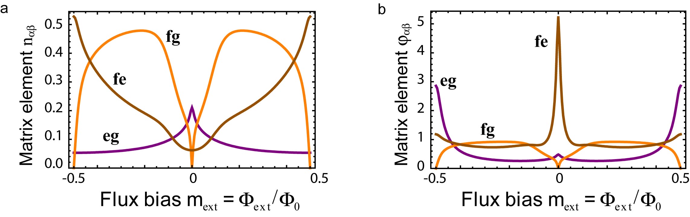
Figure 9: (a) Matrix elements of charge operator $N$ (in units of Cooper pair charge $2e$) for transitions $g\leftrightarrow e$, $g\leftrightarrow f$, and $e\leftrightarrow f$. (b) Matrix elements of phase operator (in radians) for same transitions.

A.4 Dispersive shifts of a resonator by fluxonium artificial atom

Here we evaluate $\chi_{\alpha}$ used in Eq. (9) for the reflectometry signal (Fig. 6d). The interaction of the qubit with the resonator is given by

$$\hat{V}=hg(\hat{a}+\hat{a}^{{\dagger}})\hat{n}\,,$$ (10)

where $\hat{n}$ is the charge on black-sheep junction capacitor in units of $2e$, and $\hat{a}$ is the annihilation operator for the microwave photons in the equivalent $LC$-oscillator (Fig. 6a-b). The coupling constant $g$, given by

$$g=\frac{C_{c}}{C_{J}+C_{c}}\sqrt{\frac{1}{2}Z_{0}/R_{Q}}\nu_{0}~{},$$ (11)

is expressed via the characteristic impedance of the oscillator $Z_{0}=4Z_{\infty}/\pi$ ($Z_{\infty}=70-80~{}\Omega$ is the wave impedance of the CPS transmission line), and the superconducting impedance quantum $R_{Q}=\hbar/(2e)^{2}\simeq 1~{}\mathrm{k\Omega}$. Treating $\hat{V}$ as a perturbation to second order in $g$ yields the following expression for the dispersive shift $\chi_{a}$ of the resonator frequency for the qubit in state $\left|\alpha\right\rangle$:

$$\chi_{\alpha}=2g^{2}\sum_{\beta\neq\alpha}\frac{|n_{\alpha\beta}|^{2}\nu_{\alpha\beta}}{\nu_{\alpha\beta}^{2}-\nu_{0}^{2}}\,,$$ (12)

where $n_{\alpha\beta}$ are the matrix element of the charge operator $\hat{n}$ connecting states $\alpha$ and $\beta$ and $\nu_{\alpha\beta}$ is the qubit transition frequency (in Hz) between these states. In formula 12, $\nu_{\alpha\beta}$ is taken negative if the state $\alpha$ is higher in energy than the state $\beta$, and positive otherwise; in the rest of the text, for simplicity, we treat $\nu_{\alpha\beta}$ as a positive number. Perturbation theory breaks down whenever the denominator goes to zero, a situation which corresponds to a resonance between various qubit transitions and the resonator frequency. The inset of Fig. 2c shows an uncommon instance of such vacuum Rabi resonance with the qubit transition $e\leftrightarrow f$. A conventional vacuum Rabi resonance, involving the lowest $g\leftrightarrow e$ qubit transition, takes place at $|m_{\mathrm{ext}}|\simeq 0.05$ and $\nu_{eg}\simeq 8.2~{}\mathrm{GHz}$, it is shown as an anticrossing of the theory lines (actual data available elsewhere Manucharyan2009 ).

Interestingly, for the case of the present fluxonium artificial atom, the dominant contribution to the dispersive shift of the lowest transition ($g\leftrightarrow e$) comes from the transitions $g\leftrightarrow f$ and $e\leftrightarrow f$ and not from the $g\leftrightarrow e$ transition itself. This happens because the transitions to the $f$ state involve large charge motion and the $\nu_{ef}$ frequency remains in a window $1-2~{}\mathrm{GHz}$ away from the cavity frequency $\nu_{0}$ for all flux values. This behavior is due to a large participation of the black-sheep plasma mode in the $f$ state for the present device parameters. By contrast, the $g\leftrightarrow e$ transition involves little charge motion (Fig. 9) because it connects states with different phase-slips number $m$, and, in addition, detunes quickly from the cavity with the external flux. The large splitting between the transition $e\leftrightarrow f$ and the resonator shown in the inset of Fig. 2c of the main text illustrates this point.

Appendix B Decoherence of fluxonium

B.1 Aharonov-Casher Line Broadening

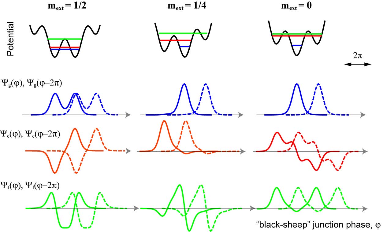
Figure 10: Top row: Effective potential for the “black-sheep” junction phase and a sketch of the three lowest levels for three values of $m_{\mathrm{ext}}$. Bottom rows: Overlap between $2\pi$-shifted fluxonium wavefunctions in states $g$, $e$, and $f$, for the three values of $m_{\mathrm{ext}}$. Note that for states $g$ and $e$ the overlap is clearly maximal when $|m_{\mathrm{ext}}|=1/2$.

Here we derive and discuss Eq. (6). The Hamiltonian of model B, defined by Eqs. (4) and (5) is invariant under the transformation $(\varphi,~{}\tilde{m})\rightarrow(\varphi-2\pi,~{}\tilde{m}+1)$. This symmetry represents the fact that by looking only at the initial and final states of the junction loop we cannot distinguish which part of the loop (black-sheep junction or the array) actually underwent a phase-slip. This point can also be illustrated by representing graphically the phase distribution of array islands before and after a phase-slip by $2\pi$(Fig. 1e). The unperturbed eigenstates $\left|\alpha\right\rangle^{(0)}$ of the Hamiltonian (4) then take the following form:

$$\left|\alpha\right\rangle^{(0)}=\lim_{M\rightarrow\infty}\frac{1}{\sqrt{2M+1}}\sum_{\tilde{m}=-M}^{M}\Psi_{a}(\varphi-2\pi\tilde{m})\left|\tilde{m}\right\rangle~{}.$$ (13)

Here $\Psi_{\alpha}(\varphi)$ is the wavefunction of the $\alpha$-th (non-degenerate) eigenstate of the fluxonium Hamiltonian Eq. (5), the states $\left|\tilde{m}\right\rangle$ are the eigenstates of the integer $\tilde{m}$ operator, and the normalization is chosen to satisfy $\left\langle\alpha|\beta\right\rangle^{(0)}=\delta_{\alpha\beta}$. Now, treating the quantum phase-slips perturbation (second term of Eq. (4)) to the first order in $|E_{S}|$, we find that the correction to the qubit transition frequency $\nu_{\alpha\beta}^{\{1\}}$ between the states $\alpha$ and $\beta$:

$$\nu_{\alpha\beta}^{\{1\}}=\frac{1}{2h}\lim_{M^{\prime},M^{\prime\prime}\rightarrow\infty}\frac{1}{\sqrt{2M^{\prime}+1}\sqrt{2M^{\prime\prime}+1}}\\ \times\sum\limits_{\tilde{m}=-\infty}^{+\infty}\sum\limits_{\tilde{m}^{\prime}=-M^{\prime}}^{M^{\prime}}\sum\limits_{\tilde{m}^{\prime\prime}=-M^{\prime\prime}}^{M^{\prime\prime}}\int\limits_{-\infty}^{\infty}\mathrm{d}\varphi\\ \times(\Psi_{\alpha}(\varphi-2\pi\tilde{m}^{\prime})\Psi_{\alpha}(\varphi-2\pi\tilde{m}^{\prime\prime})\\ -\Psi_{\beta}(\varphi-2\pi\tilde{m}^{\prime})\Psi_{\beta}(\varphi-2\pi\tilde{m}^{\prime\prime}))\\ \times\left(E_{S}\left\langle\tilde{m}^{\prime}|\tilde{m}\right\rangle\left\langle\tilde{m}+1|\tilde{m}^{\prime\prime}\right\rangle+E_{S}^{\ast}\left\langle\tilde{m}^{\prime}|\tilde{m}+1\right\rangle\left\langle\tilde{m}|\tilde{m}^{\prime\prime}\right\rangle\right)~{}.$$

Because states with $\tilde{m}\neq\tilde{m}^{\prime}$ are orthogonal, the sum reduces to a compact expression

$$\nu_{\alpha\beta}^{\{1\}}=\frac{\mathrm{Re}[E_{S}]}{h}F_{\alpha\beta}(m_{\mathrm{ext}})~{},$$ (14)

where the overlap function $F_{\alpha\beta}(m_{\mathrm{ext}})$ is defined by Eq. (7). The flux dependence of $\nu_{\alpha\beta}^{\{1\}}$ comes from the flux-dependence of the qubit state wavefunction, several examples are illustrated in Fig. 10 and in Fig. 11.

In order to convert the shift $\nu_{\alpha\beta}^{\{1\}}$, Eq. (14), into the linewidth $\delta\nu_{\alpha\beta}$, Eq. (6), let us recall that

$$E_{S}=\sum\limits_{j=1}^{N}E_{S_{j}}\exp\left(i2\pi Q_{j}/2e\right)~{},$$ (15)

with $Q_{j}$ being random variables with a spread of values comparable to $e$, and the sum running over all array junctions. According to the central-limit theorem, in the limit of large $N$, the quantity Re$[E_{S}]$ obeys to the gaussian distribution with zero meanand standard deviation $\sigma=\sqrt{\overline{(\mathrm{Re}[E_{S}])^{2}}}$,

$$P\{0<\mathrm{Re}[E_{S}]<x\}=\frac{1}{\sqrt{2\pi}\sigma}\exp(-x^{2}/2\sigma^{2})~{}.$$ (16)

Assuming the array junctions to be approximately identical, $E_{S_{j}}\simeq E_{SA}$, we get $\overline{(\mathrm{Re}[E_{S}])^{2}}=\frac{1}{2}E_{SA}^{2}\times N$, and then readily compute the linewidth $\delta\nu_{\alpha\beta}$ (defined as $\sqrt{\overline{\left(\nu_{\alpha\beta}^{\{1\}}\right)^{2}}}$) due to inhomogeneous broadening to be given by Eq. (6). If charges $Q_{j}$ vary slowly compared to the duration of a single Ramsey fringe experiment (of order $10~{}\mathrm{\mu s}$), the decaying envelope of the of Ramsey fringes is given by the absolute value of the characteristic function of the distribution (16). We therefore find that Ramsey fringe envelope is given by a gaussian $\exp\left(-\left(t/T_{\phi}^{\mathrm{CQPS}}\right)^{2}\right)$, with the flux-dependent dephasing time $T_{\phi}^{\mathrm{CQPS}}$ of the $\alpha\rightarrow\beta$ transition due to the coherent quantum phase-slips given by

$$1/T_{\phi}^{\mathrm{CQPS}}(m_{\mathrm{ext}})=\sqrt{2}\pi\delta\nu_{\alpha\beta}(m_{\mathrm{ext}})~{}.$$ (17)

We used the expression (17) to produce theory plots in Fig. 3.

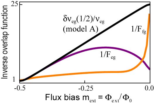
Figure 11: Flux-dependent part of the inverse linewidth due to coherent quantum phase-slips and the Aharonov-Casher effect in the array. Black line corresponds to the model A prediction for the $g\leftrightarrow e$ transition, purple and yellow lines present results of model B for the $g\leftrightarrow e$ and $g\leftrightarrow f$ transitions, respectively. Note that close to $|m_{\mathrm{ext}}|=1/2$ the two models provide the same result for the lowest transition.

B.2 Energy relaxation of fluxonium transitions ($T_{1}$ processes)

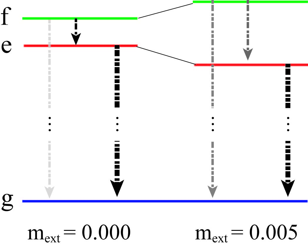
Figure 12: Sketch of the lowest three energy levels of fluxonium qubit and structure of the corresponding relaxation rates in close proximity to $m_{\mathrm{ext}}=0$. Vanishing of the phase matrix element $\varphi_{fg}$ at $m_{\mathrm{ext}}=0$ combined with the particular frequency dependence of $R_{\mathrm{intrinsic}}(\omega)$ explains the sweet-spot in $T_{1}^{fg}$ at zero flux bias.

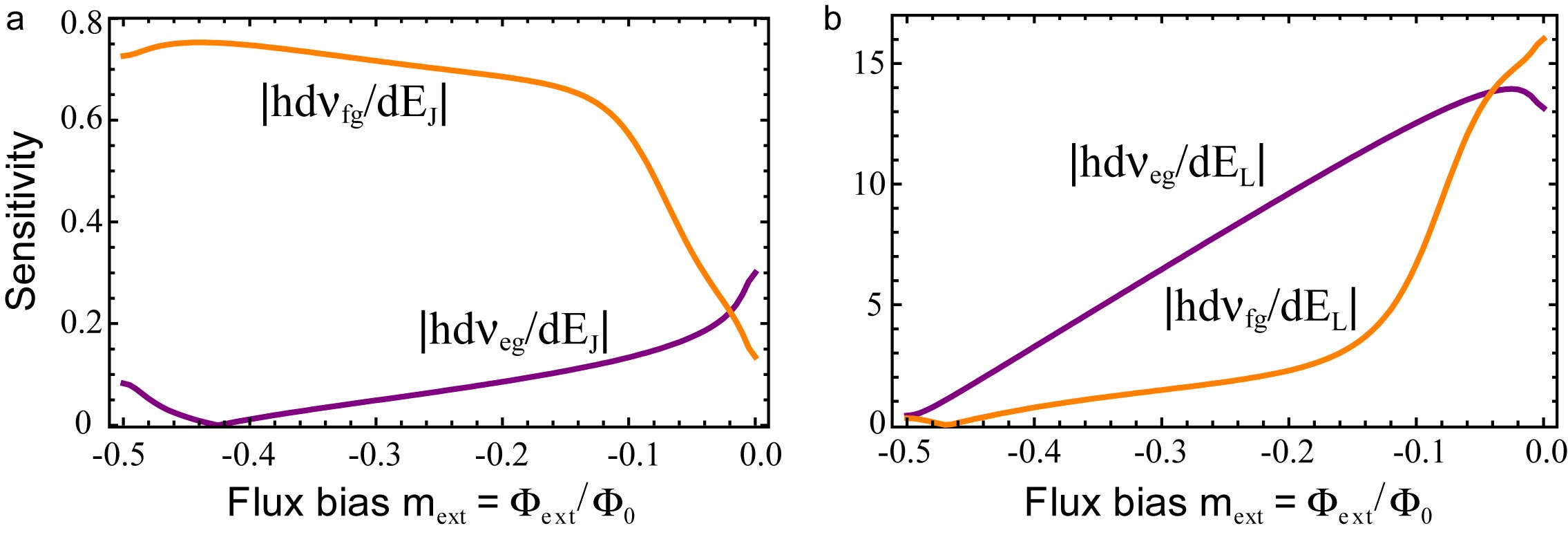
Figure 13: Sensitivity of the fluxonium spectrum to $E_{J}$ and $E_{L}$ computed numerically for the $g\leftrightarrow e$ and $g\leftrightarrow f$ transitions and present device parameters.

Transitions $e\rightarrow g$ $(g\rightarrow e)$. Energy relaxation of the qubit, taking into account the finite temperature of the sample, an important effect around $m_{\mathrm{ext}}=1/2$, takes place at the rate $\Gamma_{1}=\Gamma_{g\rightarrow e}+\Gamma_{e\rightarrow g}$, where $\Gamma_{\alpha\rightarrow\beta}$ is the rate at which the qubit makes a transition from states $\alpha$ to $\beta$. The relaxation time is defined as $T_{1}^{eg}=1/\Gamma_{1}$ and is given in terms of the black-sheep junction phase matrix element $\varphi_{eg}$ (Fig. 9b) and effective frequency-dependent parallel resistance $R_{\mathrm{eff}}(\omega)$ shunting the black-sheep junction. We may decompose this resistance into the components $R_{\mathrm{intrinsic}}(\omega)$ and $R_{\mathrm{Purcell}}(\omega)$, originating from the spontaneous emission into the dissipative bath associated with the qubit circuit, and into the measurement apparatus, respectively:

$$R_{\mathrm{eff}}^{-1}=R_{\mathrm{intrinsic}}^{-1}+R_{\mathrm{Purcell}}^{-1}~{}.$$ (18)

The latter dissipation mechanism comes from the resonator-filtered $50$ $\Omega$ environment of the measurement circuit (Fig. 7a-b) and is called Purcell effect . The resulting formula for $T_{1}^{eg}$ is obtained from Fermi’s golden rule:

$$1/T_{1}^{eg}=4\pi\frac{R_{Q}}{R_{\mathrm{eff}}(2\pi\nu_{eg})}|\varphi_{eg}|^{2}\nu_{eg}\coth\frac{h\nu_{eg}}{2k_{B}T}~{}.$$ (19)

Here,

$$R_{\mathrm{Purcell}}^{-1}(\omega)=Z_{\infty}^{-1}\frac{(\omega Z_{\infty}C_{c})^{2}}{Q_{\mathrm{ext}}}\frac{\pi}{4}\frac{\left(\omega/\omega_{0}\right)^{2}}{\cot^{2}(\frac{\pi}{2}\omega/\omega_{0})}~{},$$ (20)

is the real part of the admittance of the electrical circuit connected to the black-sheep junction. In Fig. 6a this is a circuit connected to the two terminals of the element $Z^{\left|\alpha\right\rangle}(\omega)$ with a pair of coupling capacitances $2C_{c}~{}$(the capacitances $2C_{c}$ are also shown as the interdigitated capacitances in Fig. 1a and Fig. 5c). The above expressions work as long as $|1-\nu/\nu_{0}|\gg Q_{\mathrm{ext}}^{-1}$. Note that $R_{\mathrm{Purcell}}\sim 1/C_{c}^{2}$, and that the value of $C_{c}$ in our circuit is of order $1~{}\mathrm{fF}$, making the Purcell contribution smaller than in transmon qubits ($C_{c}\approx 20~{}\mathrm{fF}$) by more than two orders of magnitude. For the parameters of our sample, the Purcell contribution becomes negligible as soon as $\nu_{0}-\nu_{eg}>300~{}\mathrm{MHz}$. Therefore, energy relaxation in our qubit is mostly intrinsic. Using the reasoning in the main text, we express $R_{\mathrm{intrinsic}}$ through the effective (and also frequency-dependent) shunting resistances $R_{j}$ of the junctions (Fig. 1b):

$$R_{\mathrm{intrinsic}}^{-1}=R_{0}^{-1}+\left(\sum\limits_{j=1}^{N}R_{j}\right)^{-1}~{}.$$ (21)

Since the area of the black-sheep junction is only a factor of $6-7$ smaller than that of the array junctions, and assuming that $R_{j}^{-1}$ is proportional to the area, it is likely that for large $N$, only the black-sheep junction ($j=0$) contributes, $R_{\mathrm{intrinsic}}\approx R_{0}$.

Relaxation $f\rightarrow g$. In the vicinity of $m_{\mathrm{ext}}=0$, we have $\Gamma_{e\rightarrow g}\gg\Gamma_{f\rightarrow e}$, $\Gamma_{f\rightarrow g}$. In the two-step transition $f\rightarrow e\rightarrow g$ the step, $f\rightarrow e$, is the bottleneck (Fig. 9b, 12). Therefore, the relaxation time associated with the $f\rightarrow g$ transition can be written as $1/T_{1}^{fg}\simeq\Gamma_{f\rightarrow e}+\Gamma_{f\rightarrow g}$, and, neglecting the Purcell contribution, we get

$$\left(T_{1}^{{}^{fg}}\right)^{-1} \simeq 4\pi\frac{R_{Q}}{R_{\mathrm{intrinsic}}(2\pi\nu_{fg})}|\varphi_{fg}|^{2}\nu_{fg}+$$ (22)

$$+4\pi\frac{R_{Q}}{R_{\mathrm{intrinsic}}(2\pi\nu_{fe})}|\varphi_{fe}|^{2}\nu_{fe}\frac{1}{1-\exp\left(-\frac{h\nu_{fe}}{k_{B}T}\right)}~{}.$$

We dropped the temperature-dependent factor in the first term because, in our experiment, in the vicinity of $m_{\mathrm{ext}}=0$, the transition energy are such that $h\nu_{fe}\approx k_{B}T\ll h\nu_{fg}$. Once $k_{B}T\simeq h\nu_{fg}$, the relaxation process becomes more complicated.

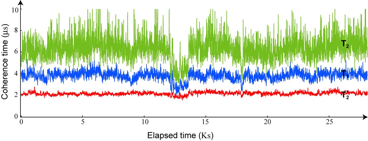
Figure 14: Measurement of $T_{1}$ (blue trace), $T_{2}^{\ast}$ (red trace) and $T_{2}$ (green trace) as a function of time for the $g\leftrightarrow e$ transition at $|m_{\mathrm{ext}}|=0.2$. A set of the three data points was acquired continuously every $8$ seconds.

B.3 Common dephasing mechanisms

Noise in $m_{\mathrm{ext}}$. We establish a higher bound on its amplitude, assuming the noise is “1/f” ($S_{m_{\mathrm{ext}}}=\delta m_{\mathrm{ext}}^{2}/\nu$, where $\nu$ is the frequency in $\mathrm{Hz}$), from pure dephasing time at $m_{\mathrm{ext}}=0.2$, where the $T_{2}^{\ast}$ is maximal (Fig. 3a) but Aharonov-Casher contribution is suppressed. For a “1/f” flux noise the pure dephasing time (gaussian decay of echo signal) is given by Nakamura

$$1/T_{\phi}^{m_{\mathrm{ext}}}\approx\delta m_{\mathrm{ext}}\times\mathrm{d}\nu_{eg}(m_{\mathrm{ext}})/\mathrm{d}m_{\mathrm{ext}}~{}.$$ (23)

We estimate the dephasing time by subtracting the decay constant $1/T_{2}$ of the echo signal (which was nearly exponential), from the separately measured $1/2T_{1}$: $T_{\phi}^{m_{\mathrm{ext}}}=(1/T_{2}-1/2T_{1})^{-1}>35~{}\mathrm{\mu s}$. Given that $\mathrm{d}\nu_{eg}(m_{\mathrm{ext}})/\mathrm{d}m_{\mathrm{ext}}\simeq 19.2~{}\mathrm{GHz}$ (Fig. 2b-c) we thus extract the “1/f” flux noise amplitude to be $\delta m_{\mathrm{ext}}<2\times 10^{-6}$.

Noise in $E_{J}\equiv E_{J_{0}}$. According to a previous studyvHarlingen , this noise is believed to be “1/f” with the spectral density $S_{E_{J}}=\delta E_{J}^{2}/\nu$, where $\delta E_{J}\propto E_{J}$. To first order, the dephasing time $T_{2}$ due to fluctuating $E_{J}$ is proportional to $\left(h\mathrm{d}\nu_{eg}(m_{\mathrm{ext}})/\mathrm{d}E_{J}\right)^{-1}$. Remarkably, present fluxonium circuit is supposed to be insensitive to the noise in $E_{J}$ for some specific value of $m_{\mathrm{ext}}\simeq 0.43$ (Fig. 13a). Overall theoretical non-monotonic dependence of $T_{2}$ on flux makes the noise in $E_{J}$ completely incompatible with the data. For instance, if the $E_{J}$ noise limits dephasing time at $m_{\mathrm{ext}}=1/2$ to the measured value of $250~{}\mathrm{ns}$, then it should also limit it to a similar number at $m_{\mathrm{ext}}\simeq 1/4$, where we measure the dephasing time one order of magnitude longer. By analogy with the flux noise relation (23), we can estimate $\delta E_{J}$ from the similar relation

$$1/T_{\phi}^{E_{J}}=\delta E_{J}\times\mathrm{d}\nu_{eg}(m_{\mathrm{ext}})/\mathrm{d}E_{J}~{}.$$ (24)

Assuming that at $m_{\mathrm{ext}}=0.2$ the pure dephasing is entirely due to “1/f” $E_{J}$ noise, we substitute $T_{\phi}^{E_{J}}>35~{}\mathrm{\mu s}$ and $h\mathrm{d}\nu_{eg}(m_{\mathrm{ext}})/\mathrm{d}E_{J}\simeq 0.1$ (Fig. 13a), we extract a conservative estimate $\delta E_{J}<3\times 10^{-5}E_{J}$.

Noise in $E_{L}$. Fluctuations in the Josephson energies $E_{J_{j\neq 0}}$ of the array junctions would result in a noisy inductance (noisy $E_{L}$) such that $S_{E_{L}}=\delta E_{L}^{2}/\nu$. Already from the considerations of model A it is clear that $\mathrm{d}\nu_{ge}(m_{\mathrm{ext}})/\mathrm{d}E_{L}$ is minimal at $m_{\mathrm{ext}}=1/2$ and maximal at $m_{\mathrm{ext}}=0$, see Eq. (3) and Fig. 1f. Calculating this derivative numerically (Fig. 13b) we conclude that the theoretical flux-dependence of the $E_{L}$ noise indeed is completely inconsistent with our dephasing data. We extract the higher bound on the $E_{L}$ noise, assuming it is 1/f, from the pure dephasing time of the $g\leftrightarrow f$ transition measured at $m_{\mathrm{ext}}=0$, where flux, $E_{J}$, and Aharonov-Casher dephasing effects are minimal (Fig. 2c, Fig. 11, and Fig. 13a). Using, as usual, $1/T_{\phi}^{E_{L}}=1/T_{2}-1/2T_{1}^{fg}$, the relation

$$1/T_{\phi}^{E_{L}}=\delta E_{L}\times\mathrm{d}\nu_{fg}(m_{\mathrm{ext}})/\mathrm{d}E_{L}~{},$$ (25)

the observed values $T_{\phi}>50~{}\mathrm{\mu s}$, and $h\mathrm{d}\nu_{fg}(m_{\mathrm{ext}})/\mathrm{d}E_{L}\simeq 16$ (Fig. 13b) at $m_{\mathrm{ext}}=0$, we find $\delta E_{L}<3\times 10^{-6}E_{L}$.

B.4 Time-stability of the decoherence times

Fig. 14 shows that the measured values of $T_{1}$ may show fluctuations by as much as $50\%$ over time. The data is taken for the lowest $g\leftrightarrow e$ transition for $m_{\mathrm{ext}}=0.2$ and is typical for any other bias. The origin of these $T_{1}$ fluctuations is unknown. Fortunately, the dephasing times $T_{2}^{\ast}$, measured in a Ramsey fringe experiment, being significantly lower than $2T_{1}$, are almost unaffected by the fluctuations in $T_{1}$. We also note that the times $T_{2}$, measured in an echo experiment, follow the fluctuations of $T_{1}$, confirming that the value of $T_{2}$ is indeed close to $2T_{1}$.

References

- (1) V. L. Ginzburg and L. D. Landau, Zh. Eksp. Teor. Fiz. 20, 1064 (1950). [L. D. Landau, Collected papers (Pergamon Press, 1965)].
- (2) B. I. Halperin, G. Refael, E. Demler, in Bardeen, Cooper and Schrieffer: 50 Years, L. Cooper and D. Feldman, eds. (World Scientific 2010).
- (3) A. D. Zaikin, D. S. Golubev, A. van Otterlo, G. T. Zimanyi, Phys. Rev. Lett. 78, 1552 (1997).
- (4) H. P. Buchler, V. B. Geshkenbein, G. Blatter, Phys. Rev. Lett. 92, 067007 (2004).
- (5) J. E. Mooij, Yu. V. Nazarov, Nature Phys. 2, 169 (2006).
- (6) K. A. Matveev, A. I. Larkin, L. I. Glazman, Phys. Rev. Lett. 89, 096802 (2002).
- (7) D. A. Ivanov, L. B. Ioffe, V. B. Geshkenbein, G. Blatter, Phys. Rev. B 65, 024509 (2001).
- (8) Y. Aharonov, A. Casher, Phys. Rev. Lett. 53, 319 (1984).
- (9) R. Fazio, H. van der Zant, Physics Reports 355, 235 (2001).
- (10) B. Doucot, J. Vidal, Phys. Rev. Lett. 88, 227005 (2002).
- (11) L. B. Ioffe, M. V. Feigel’man, Phys. Rev. B 66, 224503 (2002).
- (12) D. V. Averin, A. B. Zorin, K. K. Likharev, Zh. Exp. Teor. Phys. 88, 692 (1985). [Sov. Phys. JETP 61, 407 (1985)].
- (13) D. Haviland, K. Andersson, P. Agren, J. Low Temp. Phys. 118, 733 (2000).
- (14) A. Bezryadin, C. N. Lau, M. Tinkham, Nature 404, 971 (2000).
- (15) K. Yu. Arutyunov, D. S. Golubev, A. D. Zaikin, Phys. Rep. 464, 1 (2008).
- (16) M. Sahu, M. H. Bae, A. Rogachev, D. Pekker, T. C. Wei, N. Shah, P. M. Goldbart, A. M. Bezryadin, Nature Phys. 5, 503 (2009).
- (17) S. Gladchenko, D. Olaya, E. Dupont-Ferrier, B. Douçot, L. B. Ioffe, M. E. Gershenson, Nature Phys. 5, 48 (2009).
- (18) I. M. Pop, I. Protopopov, F. Lecocq, Z. Peng, B. Pannetier, O. Buisson, W. Guichard, Nature Phys. 6, 589 (2010).
- (19) J. E. Mooij, C. J. P. M. Harmans, New J. Phys. 7, 219 (2005).
- (20) J. E. Mooij, T. P. Orlando, L. Levitov, L. Tian, C. H. Van der Wal, S. Lloyd, Science 285, 1036 (1999).
- (21) V. E. Manucharyan, J. Koch, L. I. Glazman, M. H. Devoret, Science 326, 113 (2009).
- (22) A. Wallraff, D. I. Schuster, A. Blais, L. Frunzio, R. S. Huang, J. Majer, S. Kumar, S. M. Girvin, R. J. Schoelkopf, Nature 431, 162 (2004).
- (23) D. I. Schuster, A. Wallraff, A. Blais, L. Frunzio, R. S. Huang, J. Majer, S. M. Girvin, R. J. Schoelkopf, Phys. Rev. Lett. 94, 123602 (2005).
- (24) , in the limit of large and within the WKB approximation MLG2002 .
- (25) W. J. Elion, J. J. Wachters, L. L. Sohn, J. E. Mooij, Phys. Rev. Lett. 71, 2311 (1993)
- (26) J. R. Friedman, D. V. Averin, Phys. Rev. Lett. 88, 050403 (2002).
- (27) J. Aumentado, M. W. Keller, J. M. Martinis, M. H. Devoret, Phys. Rev. Lett. 92, 066802 (2004).
- (28) A. Hriscu, Yu. V. Nazarov, Phys. Rev. Lett. 106, 077004 (2011).
- (29) J. M. Martinis, Quantum Information Processing 8, 81 (2009).
- (30) L. Faoro, L. B. Ioffe, Phys. Rev. Lett. 96, 047001 (2006).
- (31) A. A. Houck, J. A. Schreier, B. R. Johnson, J. M. Chow, J. Koch, J. M. Gambetta, D. I. Schuster, L. Frunzio, M. H. Devoret, S. M. Girvin, R. J. Schoelkopf, Phys. Rev. Lett. 101, 080502 (2008).
- (32) F. Yoshihara, K. Harrabi, A. O. Niskanen, Y. Nakamura, J. S. Tsai, Phys. Rev. Lett. 97, 167001 (2006).
- (33) D. J. Van Harlingen, T. L. Robertson, B. L. T. Plourde, P. A. Reichardt, T. A. Crane, J. Clarke, Phys. Rev. B 70, 064517 (2004).