Thermohaline Mixing and its Role in the Evolution of Carbon and Nitrogen Abundances in Globular Cluster Red Giants: The Test Case of Messier 3

Abstract

We review the observational evidence for extra mixing in stars on the red giant branch (RGB) and discuss why thermohaline mixing is a strong candidate mechanism. We recall the simple phenomenological description of thermohaline mixing, and aspects of mixing in stars in general. We use observations of M3 to constrain the form of the thermohaline diffusion coefficient and any associated free parameters. This is done by matching [C/Fe] and [N/Fe] along the RGB of M3. After taking into account a presumed initial primordial bimodality of [C/Fe] in the CN-weak and CN-strong stars our thermohaline mixing models can explain the full spread of [C/Fe]. Thermohaline mixing can produce a significant change in [N/Fe] as a function of absolute magnitude on the RGB for initially CN-weak stars, but not for initially CN-strong stars, which have so much nitrogen to begin with that any extra mixing does not significantly affect the surface nitrogen composition.

1 Introduction

Standard stellar evolution theory predicts that only one mixing event will change the surface composition of a low-mass star as it ascends the red giant branch. That event is the so-called first dredge-up (FDU, see Iben 1967) associated with the inwards migration of the base of the convective envelope into regions where hydrogen burning via the CNO-bicycle has occurred. Relatively modest changes in surface C and N abundance are predicted, and once the convective envelope recedes outwards these changes are brought to a halt. However, observations of low-mass red giants ($M<2.5M_{\odot}$, see for example Charbonnel & Do Nascimento 1998) for essentially all compositions show trends among light element abundances that cannot be accounted for by the FDU. Some form of non-convective mixing seems to occur whereby greater amounts of the products of partial hydrogen burning are cycled into the convective envelope over a much longer timescale, and during more advanced phases of RGB evolution, than can be explained by the FDU. The observational results summarised below imply that current canonical models do not include essential physics of this so-called “extra mixing”. Regardless of what the physical mechanism is, extra mixing is required to conform to the following observational criteria:

1. It commences after the hydrogen burning shell has erased a composition discontinuity in the radiative zone that marked the innermost limit of the convective envelope during the FDU event, and may continue to at least the tip of the RGB (Gilroy & Brown, 1991; Charbonnel et al., 1998; Gratton et al., 2000; Smith & Martell, 2003; Shetrone, 2003; Weiss & Charbonnel, 2004; Martell et al., 2008). The onset of the extra mixing is thus thought to coincide with a local maximum (the so-called “bump”) observed in the RGB luminosity function of globular clusters.

2. It must occur over a range of masses and metallicities (Smiljanic et al., 2009, and references therein), being active in giants of all metallicities from solar to at least [Fe/H] $\sim-2.5$ (Gratton et al., 2000) and masses less than $\sim 2.5M_{\odot}$ (Lambert & Ries, 1977), although not necessarily with equal efficiency throughout these mass and metallicity ranges.

3. It must deplete ${}^{7}\mathrm{Li}$ (Charbonnel et al., 1998; Smiljanic et al., 2009; Lind et al., 2009).

4. It must decrease the ${}^{12}\mathrm{C}$/${}^{13}\mathrm{C}$ ratio (Charbonnel, 1994, 1996), since values lower than predicted by the FDU are found among Population I field giants (Tomkin et al., 1976; Lambert & Ries, 1981; Charbonnel et al., 1998), open cluster giants (Gilroy, 1989; Gilroy & Brown, 1991; Smiljanic et al., 2009; Mikolaitis et al., 2010), globular cluster giants (Shetrone, 2003; Recio-Blanco & de Laverny, 2007) and halo field giants (Sneden et al., 1986; Gratton et al., 2000).

5. It must decrease the total carbon abundance since systematic decreases with advancing luminosity on the upper half of the red giant branch are seen both among globular clusters and halo field giants (Suntzeff, 1981, 1989; Carbon et al., 1982; Trefzger et al., 1983; Langer et al., 1986; Gratton et al., 2000; Bellman et al., 2001; Smith & Martell, 2003; Martell et al., 2008; Shetrone et al., 2010). In Population II giants the behaviour of the carbon abundance can serve as an even more potent probe of the extent of extra mixing than the ${}^{12}\mathrm{C}$/${}^{13}\mathrm{C}$ isotope ratio, because the latter can attain near-equilibrium values for only moderate amounts of mixing that would otherwise cause only small ($\sim$0.1 dex) changes in [C/H] (Sneden et al., 1986).

6. As a consequence of the previous point it must increase the nitrogen abundance. The results of CN cycling are observed on the upper half of the red giant branch. Halo field stars on the upper RGB were found by Gratton et al. (2000) to show an excess of nitrogen compared to those on the lower RGB.

It is expected that the mechanism(s) will also destroy ${}^{3}\mathrm{He}$ inside the star (Dearborn et al., 1986; Hata et al., 1995; Dearborn et al., 1996; Sackmann & Boothroyd, 1999; Charbonnel & Zahn, 2007a, b). As we cannot observe ${}^{3}\mathrm{He}$ in stellar atmospheres directly this is not an observational constraint, but it is a significant requirement from the study of chemical yields and galactic evolution. The importance of ${}^{3}\mathrm{He}$ is discussed in Section 3.

In the last four decades many candidate extra-mixing mechanisms have been suggested. These include: rotational mixing (Sweigart & Mengel, 1979; Chanamé et al., 2005; Palacios et al., 2006), magnetic fields (Palmerini et al., 2009; Nordhaus et al., 2008; Busso et al., 2007), and internal gravity waves (Denissenkov & Tout, 2000). Individually, none of these have been proven to be satisfactory. Due to its promising ability to account for the above requirements, and the necessity of its occurrence in low mass giants just after the FDU, in this study we focus on ${}^{3}\mathrm{He}$-driven “thermohaline mixing” (Eggleton et al. 2006, EDL06 hereafter, Charbonnel & Zahn 2007a, CZ07a hereafter, Eggleton et al. 2008, EDL08 hereafter). The name comes from a phenomenon seen in oceans, and is taken from the two major determinants of the density of sea water - its heat content (“thermo”) and its salinity (the salt or “haline” content). It is common to find warm salty water overlying cool fresh water. Although the higher salinity of the warm water makes it denser, the higher heat content acts to stabilise the stratification. The subsequent evolution of the system is determined by the competition between two diffusion processes and their associated timescales - the time for the (stabilizing) heat to diffuse away compared to the time for the (destabilizing) salt to do the same. Hence the process is often called “doubly-diffusive”, and it has been studied in the oceanographic context for many years (see recent reviews, theoretical modelling, observations and laboratory experiments in Progress of Oceanography Volume 56, 2003; e.g. Ruddick & Gargett 2003). Within oceans it is now well known that the rapid diffusion of heat from the warm salty layer produces an over-dense layer that begins to sink into the cooler fresh water below. The temperature stays roughly the same as the surrounds, and “salt fingers” form which extend downward delivering the saltier water to deeper regions. Reciprocal fresh-water fingers move upward and replace the salty water with fresher water. Laboratory experiments have also played a role in helping to characterise the instability. Work by Stommel and Faller published in Stern (1960) as well as more recently Krishnamurti (2003, and references there in) have helped elucidate the instability.

A similar process can occur in stars. Here it is not salt but the mean molecular weight that is the “destabilising agent”, in the words of Denissenkov (2010). Usually, the molecular weight increases as we move toward the centre of the star, as a result of nuclear burning and fusion reactions. If it were to decrease, then the plasma would be buoyantly unstable, just as is the case in convection. However, just as in the oceanic case, we must include the rapid thermal diffusion which can act to stabilise the motion. In this paper we consider the situation where some local event causes a decrease in the molecular weight in an otherwise stable region within a star. We investigate the effects of the resultant “thermohaline mixing” or doubly diffusive process that is initiated by a molecular weight ($\mu$) inversion (Ulrich, 1972; Kippenhahn, Ruschenplatt & Thomas, 1980).

Recently thermohaline mixing has featured prominently in the literature. EDL06, CZ07a, EDL08, Cantiello & Langer (2010) and Charbonnel & Lagarde (2010) have discussed in detail the important consequences of its inclusion during the RGB. The dichotomy in RGB carbon abundance between metal poor stars and carbon-enhanced metal-poor stars has been explained by Stancliffe et al. (2009) using thermohaline mixing. Cantiello & Langer (2010), Stancliffe (2010) and Charbonnel & Lagarde (2010) have shown that its operation beyond the giant branch may affect the subsequent asymptotic giant branch (AGB) evolution. This mechanism may be a crucial part of stellar physics that has been missing from the models. We thus believe it pertinent to investigate the effects of the mechanism in some detail.

In this paper we will take the approach of trying to model the mixing in spherically symmetric stellar models and investigate its effect on observable surface abundances. In this respect our approach follows that of CZ07a and Charbonnel & Lagarde (2010). We will examine the change of the abundances of carbon and nitrogen on the red giant branch of globular clusters, focusing on the case of M3.

Currently a range of approaches is taken to include thermohaline mixing in evolution codes, especially if the ${}^{12}\mathrm{C}$/${}^{13}\mathrm{C}$ ratio is the constraint used to determine the extent of extra mixing. The ${}^{12}\mathrm{C}$/${}^{13}\mathrm{C}$ ratio was one of the first indicators that extra mixing must operate on the RGB. It is classically used to probe the results of FDU (Dearborn et al., 1975; Tomkin et al., 1976; Charbonnel, 1994). It naturally follows that the ${}^{12}\mathrm{C}$/${}^{13}\mathrm{C}$ ratio could be used to trace the extent of extra mixing and constrain any mechanism. The change in ${}^{12}\mathrm{C}$/${}^{13}\mathrm{C}$ ratio following FDU will depend on the efficiency of mixing and allow us to explore the mixing velocity via a diffusion approximation. EDL08 estimated the mixing speed with their formula for the diffusion coefficient and found that a range of three orders of magnitude in their free parameter can lead to the observed levels of ${}^{12}\mathrm{C}$/${}^{13}\mathrm{C}$ and ${}^{3}\mathrm{He}$ depletion. Ulrich (1972) and Kippenhahn, Ruschenplatt & Thomas (1980) both use essentially the same formula (UKRT formula hereafter) for the diffusion coefficient but their choice of the free parameter varies by two orders of magnitude. In an attempt to constrain the parameter space we address the following questions:

1. The ${}^{12}\mathrm{C}$/${}^{13}\mathrm{C}$ ratio is generally used as a tracer to probe the extent of mixing. This ratio saturates near the CN equilibrium value rather quickly in low metallicity stars, and hence is of limited utility. Is there a better way to constrain the mixing?

2. Which formalism should be used? Here we will limit our investigation to the EDL08 and UKRT prescriptions for the diffusion coefficient.

3. Once the preferred formalism is identified, what diffusion co-efficient (or mixing velocity) is needed to match observations? What values do we use for any free parameters?

As has been the practice for many years, we turn to globular clusters to test our understanding of stellar theory. Smith (2002), Smith & Martell (2003) and Martell et al. (2008) have compiled observations of carbon and nitrogen along the giant branch of M3. This has provided us with a valuable alternative to the ${}^{12}\mathrm{C}$/${}^{13}\mathrm{C}$ probe. By matching our models to the carbon depletion (as a function of absolute magnitude) observed in this cluster we can attempt to constrain both the form of the thermohaline diffusion coefficient and the values of any parameters contained therein. As carbon and nitrogen are intrinsically linked in the CN burning cycle we include observations of nitrogen as an additional tracer. Furthermore, we identify when extra mixing begins in the models and compare this to the observed luminosity function bump (LF bump) in the cluster.

2 Thermohaline Mixing

The usual condition for convective instability is simply that a blob moved from its equilibrium position will be buoyantly unstable and continue to move away from its initial position. In a region of homogeneous chemical composition this results in the usual Schwarzschild criterion for instability:

$$\nabla_{\rm{rad}}>\nabla_{\rm{ad}},$$ (1)

where $\nabla_{\rm{ad}}=(\partial\ln T/\partial\ln P)_{\rm{ad}}$ is the adiabatic gradient and $\nabla_{\rm{rad}}=(\partial\ln T/\partial\ln P)_{\rm{rad}}$ is the same gradient assuming all the energy is carried by radiation (one usually uses the diffusion approximation for this expression). This equation simply says that the steepest stable gradient is the adiabatic one, and if a steeper gradient is required to carry the energy by radiation, then radiation will fail and buoyancy will develop.

This condition however ignores the possibility of a variation in the chemical composition. Including this leads to the Ledoux criterion for instability:

$$\nabla_{\rm{rad}}>\nabla_{\rm{ad}}+\left(\frac{\varphi}{\delta}\right)\nabla_{\rm{\mu}},$$ (2)

where $\varphi=(\partial\ln\rho/\partial\ln\mu)_{P,T}$, $\delta=-(\partial\ln\rho/\partial\ln T)_{P,\mu}$ and $\nabla_{\rm{\mu}}=(\partial\ln\mu/\partial\ln P).$ The essential feature here is the appearance of the term involving the gradient of the molecular weight (the multiplicative terms $\phi$ and $\delta$ come from the thermodynamics and are of little importance for the present discussion; both are unity for a perfect gas without radiation pressure).

For thermohaline mixing we need the Ledoux criterion to be broken, but with the added condition that the molecular weight gradient decreases with depth, i.e.

$$\nabla_{\rm{\mu}}<0.$$ (3)

Thermohaline mixing has a long history. Stothers & Simon (1969) were the first to consider how thermohaline mixing may impact upon the structure and subsequent evolution of a star. They theorised that accreted material from a helium-rich companion would be thermohaline unstable and may be responsible for the pulsations of $\beta$ Cepheids.

Soon after Abraham & Iben (1970) and Ulrich (1971) recognised an unusual property of the reaction

$$^{3}\mathrm{He}\left({}^{3}\mathrm{He},2\rm{p}\right)^{4}\mathrm{He},$$ (4)

which is that despite being a fusion reaction, it actually reduces the mean molecular weight because it produces three particles from two. (These particles also have more kinetic energy than the initial two particles, because the reaction is exothermic.) They thought the reaction may have an important role during pre-main-sequence contraction, and could lead to the situation where $\nabla_{\mu}<0$ and a thermohaline instability may develop. This was later found to have little effect due to the short time scale of the pre-main-sequence.

Ulrich (1972) was the first to derive an expression for the turbulent diffusivity in a perfect gas. He considered thermohaline mixing during the core flash where off-centre ignition leads to carbon-rich material sitting on material that is helium-rich. Kippenhahn et al. (1980) extended this to allow for a non-perfect gas which included radiation pressure and degeneracy. Thermohaline mixing is unlikely to have an appreciable effect during the core flash because of the very short timescale of the flash. Dearborn et al. (2006) showed that a small amount of overshooting inwards could remove the molecular weight inversion on a dynamical timescale, thus removing the possibility of any thermohaline mixing.

3 Thermohaline Mixing on the First Giant Branch

A further application, and the one of interest to us here, was proposed by EDL06. During main-sequence evolution a low mass star produces a substantial amount of ${}^{3}\mathrm{He}$. Close to the centre all of the ${}^{3}\mathrm{He}$ has been destroyed in completing the pp chains. But at lower temperatures the ${}^{3}\mathrm{He}$ remains (e.g. see Fig 1 of EDL08). When the FDU occurs it mixes the envelope abundances over a large region, producing a homogeneous envelope with a ${}^{3}\mathrm{He}$ content that is far above the equilibrium value. Following FDU, the convective envelope recedes, leaving behind a region that is homogeneous in composition.

When the hydrogen burning shell advances, the fragile ${}^{3}\mathrm{He}$ begins to burn and the resulting decrease in the molecular weight leads to an inversion developing. Note that ${}^{3}\mathrm{He}$ burning alone is not sufficient to drive the mixing. Whenever there is hydrogen burning via the pp chains the ${}^{3}\mathrm{He}$ + ${}^{3}\mathrm{He}$ reaction (Equation 4) will decrease $\mu$. However the combined effect of the other reactions and the low abundance of ${}^{3}\mathrm{He}$ makes the effect of the ${}^{3}\mathrm{He}$ + ${}^{3}\mathrm{He}$ reaction negligible. If one can homogenise the region beforehand, then the effect of ${}^{3}\mathrm{He}$ + ${}^{3}\mathrm{He}$ dominates. This way thermohaline mixing is initiated at essentially the same luminosity as the bump in the luminosity function, since both are caused by the H-shell reaching the abundance discontinuity left behind from FDU.

From equation (4) it can be shown that the change in $\mu$ must be (EDL08)

$$\delta\mu=\mu^{2}\delta(X(^{3}\mathrm{He}))/6.$$ (5)

and they found the magnitude of such inversions to be of the order ${\Delta\mu}/{\mu}$ $\sim$ 10^-4. Although this seems small, convection is in fact driven by a similarly small superadiabaticity.

We now try to understand what happens to the material in this region of the star. When ${}^{3}\mathrm{He}$ burns, a parcel forms that is slightly hotter and has lower molecular weight than its surroundings. This means it has a higher pressure than it requires for its position. Hence it quickly expands (and begins to cool) in order to establish pressure equilibrium. The expansion reduces the density and therefore the element becomes buoyant. The parcel rises until it finds an equilibrium point where the external pressure and density are equal to that inside the bubble. This is expected to be a small displacement which occurs on a dynamical timescale.

As the molecular weight inside the bubble is lower than its surroundings the equilibrium point must correspond to a place where the external temperature is higher than that of the bubble. The temperature inside the bubble will be lower than its surroundings (we may assume a perfect gas equation of state):

$$\rm{\frac{T_{i}}{T_{o}}=\frac{\mu_{i}}{\mu_{o}}},$$ (6)

where subscript i denotes the inside of the bubble and subscript o denotes the surroundings. As heat begins to diffuse into the parcel, we expect layers will start to strip off in the form of long fingers. It is this secondary mixing that governs the overall mixing timescale. The mixing cycles in fresh ${}^{3}\mathrm{He}$ from the envelope reservoir, to replace the ${}^{3}\mathrm{He}$-depleted material that is rising toward the star’s convective envelope. This upward-flowing material will also have experienced other burning, such as CN cycling, while in the hotter region. It will also experience further burning in the future as the material is cycled through this region on subsequent occasions.

The diffusion of heat and composition is analogous to the situation in the oceans where haline fingers diffuse salt and heat, although in the stellar context we are dealing with a compressible flow. For a thorough investigation of the differences between the oceanic and stellar case we refer to Denissenkov (2010). The fact that in both instances there are two diffusive processes at work has seen the term ‘thermohaline’ adopted in the astrophysics literature (e.g. CZ07a).

As stated above, EDL08 originally referred to thermohaline mixing on the RGB as “$\delta\mu$ mixing” to distinguish and emphasise the mechanism that drives the mixing, namely the slight difference in the molecular weight brought about by ${}^{3}\mathrm{He}$ burning. Their simulations seemed to hint at the possibility of a dynamical phase in addition to the linear phase which CZ07a modelled as UKRT thermohaline mixing.

Many groups have realised the importance of understanding the mixing and are investigating the instability that arises from the ${}^{3}\mathrm{He}$ burning. The anlysis by Denissenkov & Pinsonneault (2008) of the mixing suggests a dynamical phase should not arise. Further complicating the picture are the 2D models by Denissenkov (2010) that predict a different behaviour in the fluid compared to the 1D parameter fitting of CZ07a.

We consider $\delta\mu$ mixing to be a strong extra-mixing candidate along the RGB as it can meet the criteria outlined in the introduction (CZ07a, EDL08). To summarise, this ${}^{3}\mathrm{He}$ burning drives mixing that begins after the hydrogen shell encounters the composition discontinuity left behind by FDU. We note that the depletion of ${}^{3}\mathrm{He}$ is required to ensure that stellar nucleosynthesis and Big Bang Nucleosynthesis remain consistent (Dearborn et al., 1986; Hata et al., 1995; Dearborn et al., 1996; Sackmann & Boothroyd, 1999; Charbonnel & Zahn, 2007a, b). Measurements of ${}^{3}\mathrm{He}$ in HII regions and planetary nebula (Rood et al., 1984; Hogan, 1995; Charbonnel, 1995; Charbonnel & Do Nascimento, 1998; Tosi, 1998; Palla et al., 2000; Romano et al., 2003) match the predicted yields from Big Bang Nucleosynthesis. Canonical models predict that low-mass, main-sequence stars are net producers of ${}^{3}\mathrm{He}$ which is returned to the ISM through mass loss. Hata et al. (1995) have shown that about 90% of the ${}^{3}\mathrm{He}$ produced on the main sequence must be destroyed to reconcile the two fields. We saw above how these stars produced ${}^{3}\mathrm{He}$, and the newly discovered mechanism now also destroys it, removing the inconsistency with Big Bang Nucleosynthesis. This will still allow for the existence of the minority of planetary nebula that show large ${}^{3}\mathrm{He}$ abundances (Balser et al., 1997; Balser et al., 1999, 2006; Charbonnel & Zahn, 2007b).

The thermohaline mixing mechanism described here will operate until the ${}^{3}\mathrm{He}$ is destroyed, which may be beyond the tip of the RGB (Stancliffe, 2010; Cantiello & Langer, 2010; Charbonnel & Lagarde, 2010). The molecular weight inversion caused by the ${}^{3}\mathrm{He}$ burning creates an instability that cycles CN processed material into the envelope, having the desired effect on the surface abundances (CZ07a). Finally CZ07a, EDL08 and Charbonnel & Lagarde (2010), demonstrated that the degree of mixing depends on mass and metallicity, most clearly seen in the different values of the carbon isotopic ratio in Population I and Population II stars.

4 The Formula for the Diffusion Coefficient

It is common in stellar interior calculations to use a diffusion equation to simulate mixing. It is important to remember that many mixing processes, such as convective mixing, are advective in nature, not diffusive. In the former, a property is distributed as a result of bulk flows within the fluid. The latter follows from Fick’s first law, which postulates that a flux exists between regions of high and low concentration of the quantity of interest. The equation governing this is

$$\vec{j}=-D\vec{\nabla}n$$ (7)

where $n$ is the density of the quantity and $\vec{j}$ is its flux. The parameter D is the “diffusion coefficient” of the “diffusivity”. For particles with a mean-free-path $l$ and typical speed $v$ then

$$D={1\over 3}vl.$$ (8)

As no theory for time dependent mixing exists, it is common to use a diffusion equation to simulate mixing in stellar interiors. Historically, this is also how thermohaline mixing has been calculated. A diffusion equation is solved for each species in the star, and thus determines the radial composition variation.

EDL08 used the following formula, based on estimates of the mixing velocity and the convective formalism in their evolution code:

$$D=\left\{\begin{array}[]{ccc}\frac{{F_{\rm inv}}r^{2}}{{t_{\rm nuclear}}}{\thinspace}(\mu-\mu_{\rm min})&\mbox{ if }(k\geq k_{\rm min})\\ \\ 0&\mbox{ if }(k\leq k_{\rm min}),\end{array}\right.$$ (9)

where $k$ is the mesh point number, counted outwards from the centre of the model, $k_{\rm{min}}$ is the value of $k$ for which $\mu$ takes its minimum value of $\mu_{\rm{min}}$, $r$ is the radial coordinate, $F_{\rm{inv}}$ is a constant which is selected to obtain the desired mixing efficiency and ${t_{\rm nuclear}}$ is an estimate of the nuclear evolution timescale (see EDL08). This is an extension of the convective formula used in the EDL08 calculations, with the addition of a $\mu-\mu_{\rm{min}}$ term to reflect the driving by the $\mu$ inversion. Thus this formula is not a local one as the value of $D$ at a point in the star depends on the value of $\mu_{\rm{min}}$ at some other location in the star. Nevertheless, it is a phenomenological form that recognises the role of the $\mu$ inversion in driving the mixing.

This formulation ensured the correct region was mixed but note that the mixing speed is formally zero at the position where $\mu$ has its minimum even though the mixing should presumably be the most efficient at this point. EDL08 give upper and lower estimates for the mixing velocity and find that they can change their free parameter $F_{\rm{inv}}$, and consequently alter the speed by three orders of magnitude whilst still producing the observed levels of ${}^{12}\mathrm{C}$/${}^{13}\mathrm{C}$ and leading to ${}^{3}\mathrm{He}$ depletion.

CZ07a adopt the UKRT formulation for thermohaline mixing, which results from a linear analysis of the problem. They cast it in the following way,

$$D_{t}=C_{t}\,K\left({\varphi\over\delta}\right){-\nabla_{\mu}\over(\nabla_{\rm ad}-\nabla)}\quad\hbox{for}\;\nabla_{\mu}<0,$$ (10)

where K is the thermal diffusivity and $C_{t}$ is a dimensionless free parameter. In fact $C_{t}$ is related to the aspect ratio, $\alpha$, of the fingers in the following manner:

$$C_{t}={8\over 3}\pi^{2}\alpha^{2}$$ (11)

The appropriate value to use for this parameter remains uncertain. To understand thermohaline mixing fully clearly requires a hydrodynamic theory that will determine the diffusion coefficient and any associated parameters. In lieu of such a theory, we can compare with observations and see what form of $D$ and values of constants are needed to match the real world. This is the approach we adopt in this paper.

Alternatively, one could try to determine $C_{t}$ or $\alpha$ by comparison to laboratory experiments and the oceanic case, which has been well studied. Stommel and Faller carried out experiments of fluids in laboratory conditions. This work, published in Stern (1960), saw the development of long salt fingers with lengths that were larger than their diameters ($\alpha$ $\simeq$5). This led Ulrich (1972) to determine that $C_{\rm{t}}$ $\simeq$ 658 which was the basis of the choice by CZ07a to use $C_{\rm{t}}=1000$. The huge differences between incompressible salty water and the the self-gravitating plasma we are considering make direct comparisons very difficult, however (see Denissenkov 2010). In contrast to the oceanic case, Kippenhahn envisaged the classical picture where mixing is due to blobs. If Kippenhahn’s expression is cast into the same form as Equation 10 then $C_{\rm{t}}$ $\simeq$ 12. This value seems to agree with the 2D-hydrodynamical models of Denissenkov (2010) and 1D models of Cantiello & Langer (2010), but is inconsistent with the value preferred by CZ07a and the present work (see below).

5 Models and Results

Messier 3 was chosen as a test case for thermohaline mixing in Population II stars because in many respects it can be considered a typical globular cluster. A metallicity of [Fe/H] $=-1.4$ (Sneden et al., 2004; Cohen & Meléndez, 2005) means that it falls near the mode in the metallicity distribution of halo globular clusters. Among clusters of similar metallicity, the horizontal branch morphology of M3 has stars on both the red and blue sides of the RR Lyrae gap (Sandage, 1970; Buonanno et al., 1994), and the colour distribution is intermediate between extremes such as those of M13 and NGC 6752 (whose HBs have more extended blue tails; Newell 1970; Lee & Cannon 1980) and NGC 7006 (whose HB stars are more concentrated to the red side of the RR Lyrae gap; Sandage & Wildey 1967). Red giants with enhanced $\lambda$3883 CN bands in their spectra were discovered in M3 by Suntzeff (1981), and further studied by Norris & Smith (1984). The CN distribution contains both CN-strong and CN-weak giants (i.e., high and low nitrogen abundance giants) as is typical of other clusters of similar metallicity (Norris & Smith, 1984). The behaviour of the CN bands at a given luminosity on the RGB appears to anticorrelate with carbon and oxygen abundance (Suntzeff, 1981; Smith et al., 1996). When giants of different luminosity are compared a significant trend becomes apparent in the carbon abundance. Among red giants with absolute magnitudes brighter than the horizontal branch [C/Fe] declines with increasing luminosity (Suntzeff, 1981, 1989; Smith, 2002) in a manner that is typical of other globular clusters and halo field giants (Smith & Martell, 2003). It is this behaviour of carbon in particular that is of great use in constraining models of thermohaline mixing. The carbon isotope ratio ¹²C/¹³C has a low value of $\sim$ 4-6 among the bright giants (Pilachowski et al., 2003; Pavlenko et al., 2003), although the number of stars for which this has been measured is small. In addition, M3 displays O, Na, and Al abundance inhomogeneities of the type that are commonplace within globular clusters of similar metallicity (Carretta et al., 2005). The cluster has a population of stars that are enhanced in Na and Al but depleted in oxygen (Kraft et al., 1992; Cavallo & Nagar, 2000; Sneden et al., 2004; Cohen & Meléndez, 2005; Johnson et al., 2005), but without the extremes in O abundance depletion and Na enhancement that are found in the oft-compared cluster M13 (Sneden et al., 2004). A substantial component of the O-Na-Al variations in M3 are arguably the products of early cluster self-enrichment, and thermohaline mixing on the first ascent giant branch is not expected to have played a role in their production. Work by CZ07a and Charbonnel & Lagarde (2010) also show that these elements are not affected by thermohaline mixing.

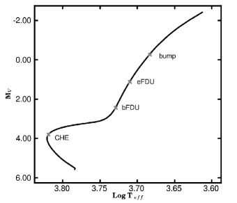
Figure 1: HR Diagram for our star that models M3. We mark: core hydrogen exhaustion (CHE) and the beginning of FDU (bFDU) which we define as the point where the penetration of the envelope begins to affect the surface abundances. Also marked is the end of FDU (eFDU) and the bump, after which extra mixing is expected to begin.

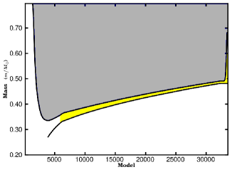
Figure 2: A simplified Kippenhan plot for our model star. We plot the interior of the star in mass co-ordinates against model number which is a non-linear proxy for time. The grey shaded region shows the penetration of the convective envelope, its deepest point coinciding with the end of FDU. We also mark the top of the hydrogen-burning shell. Unshaded regions denote radiative zones, whilst the shaded region between the shell and the envelope represents the location where thermohaline mixing occurs in the star. Although not obvious on this scale there is still a small radiative buffer between the top of the shell and the thermohaline mixed regions. Thermohaline mixing has the effect of extending the convection zone and allows material to be mixed closer to the shell where it can be processed.

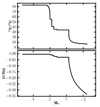
Figure 3: Top panel: ¹²C/¹³C as a function of magnitude. Bottom panel: [C/Fe] as a function of magnitude. In this figure we compare the evolution of [C/Fe] to that of ¹²C/¹³C. The UKRT thermohaline mixing formula with C_t=1000 has been used in this model. It can be seen that the isotopic ratio reaches equilibrium soon after the onset of extra mixing, where as [C/Fe] depletes along the entire RGB.

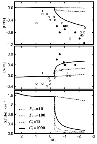
Figure 4: Abundances as a function of visual magnitude. In this figure we compare the UKRT prescription for the diffusion coefficient to that of EDL. Open circles denote CN-weak stars in M3, filled circles denote CN-strong stars and crosses represent stars of intermediate CN strength, with all data taken from Smith (2002). The two UKRT models correspond to the dashed line for C_t=12 and the solid line for C_t=1000. The two EDL models are denoted by the dotted line for $F_{\rm{inv}}$=100 and the dot dashed line for $F_{\rm{inv}}$=10, these sit nearly on top of each other on this scale. The models are all of mass $M$=0.8$\rm{M}_{\odot}$ and $Z$=5 $\times$ 10^-4 with solar scaled CNO abundances. The errors in magnitude are smaller than the symbols used. The maximum error in [C/Fe] and [N/Fe] is $\pm 0.3$ dex.

We use MONSTAR (The Monash version of the Mt.Stromlo evolution code; see Campbell & Lattanzio 2008) to produce stellar models for M3. The stars are evolved from the zero-age main-sequence until the core flash. They are of mass M=0.8 $\rm{M}_{\odot}$, metallicity Z=0.0005 and have a solar-scaled CNO abundance, as a first approximation. Population II subdwarfs in the globular cluster metallicity range tend to have [C/Fe] $\sim 0$ (e.g. Laird 1985). In M13 the work of Briley et al. (2004) shows an upper envelope to the data that approaches [C/Fe] $\sim 0$ to $-0.2$ near the main sequence.

Our mixing length parameter $\alpha$ is set to 1.75 and we run without any overshoot. Mixing is calculated using a diffusion equation, and we investigate different formulae for the diffusion co-efficient used for thermohaline mixing. These parameters approximate the stars in M3 quite well: M3 has an age estimated by various authors to be between 11.3 to 14.2 Gyr (Chaboyer et al., 1992; Jimenez et al., 1996; VandenBerg, 2000; Salaris & Weiss, 2002; Alves et al., 2004) and [Fe/H]=$-$1.5. Figure 1 shows the evolution of our model star in the HR Diagram. We mark the end of core H exhaustion (CHE in the figure, at an age of t$=$12.5 Gyr), the beginning and end of FDU (bFDU and eFDU respectively) as well as the position of the LF bump. Figure 2 shows a Kippenhahn diagram for the evolution of our star. Here we see the convective envelope moving inwards (coinciding with the beginning of FDU), whilst the deepest point of penetration marks the end of FDU. The location of thermohaline mixing is the lightly shaded region between the envelope and the advancing hydrogen burning shell. In Figure 3, using the UKRT formulation for thermohaline mixing and C_t=1000, we plot the variation of the surface [C/Fe] as well as the ¹²C/¹³C ratio versus $M_{V}$. Here it can clearly be seen that the ¹²C/¹³C ratio drops below 10 very quickly, finally reaching as low as 6.5. This is in good agreement with the observations of 4-6 by Pilachowski et al. (2003) and Pavlenko et al. (2003). The gradual depletion of carbon throughout the entire RGB on the other hand provides a more sensitive constraint on the mixing.

Figure 4 compares the results with the EDL08 and UKRT formulae for the diffusion coefficient. In this figure open circles denote CN-weak stars, filled circles denote CN-strong stars and crosses represent CN-intermediate stars all from M3. In this figure as well as the proceeding figures the errors in magnitude are smaller than the symbols used. The random errors in the abundance measurements can be up to $\pm 0.3$ dex according to Suntzeff (1981), although this does not take into account potential systematic errors due to limitations in the stellar atmospheres code used in the abundance derivations. We have run four models to compare to the observations, two with thermohaline mixing that use the UKRT formula for the diffusion coefficient and two models that use the EDL08 formula. The dashed line and the solid line are variations of the UKRT prescription, the broken line uses C_t=12 ($\alpha\sim 1$) as suggested by Kippenhahn et al. (1980) while the model represented by the solid line uses C_t=1000 ($\alpha\sim 6$), a geometry more akin to CZ07a. The dotted and dot-dashed lines (which nearly sit on top of each other) are EDL08 models where $F_{\rm{inv}}$=100 corresponds to the dotted line and $F_{\rm{inv}}$=10 corresponds to the dot-dashed line. The two choices of $F_{\rm{inv}}$ lie within the three orders of magnitude that lead to the required level of ${}^{12}\mathrm{C}$/${}^{13}\mathrm{C}$ depletion as discussed in EDL08.

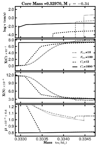
Figure 5: Various profiles for the same models as Figure 4. The same symbols are used. The profiles are all taken at the same stage in evolution, that is when the hydrogen-exhausted core mass $M_{\rm{c}}$=0.32970 $\rm{M}_{\odot}$ and at and $M_{V}=-0.34$. Top Panel: the mixing velocity in the region above the shell. Second Panel: the carbon abundance in the region above the shell. Third Panel: the nitrogen abundance in the region above the shell. Bottom Panel: highlights the respective locations where the minimum value of $\mu$ occurs.

The two EDL08 models destroy the available ${}^{3}\mathrm{He}$ very quickly and are unable to cycle much CN processed material to the envelope. As previously mentioned, in the EDL08 formulation of the diffusion coefficient the mixing is dependent on the difference in $\mu$, i.e. $(\mu-\mu_{\rm{min}})$. Material near the envelope is cycled down faster and the mixing becomes less efficient closer to the location where $\mu$ has its minimum. Material is not replenished at the same rate it would be with a local condition on the $\mu$ gradient as seen with the UKRT prescription. This in turn affects the depth at which the minimum value of $\mu$ occurs. We can see in Figure 5 that the location at which $\mu$ has its minimum occurs further out in the EDL08 scheme. The steep temperature gradient ensures the fragile ${}^{3}\mathrm{He}$ is easily destroyed while the carbon-rich material is not exposed to temperatures where it can burn significantly. CN cycling is therefore reduced whilst the driving fuel, ${}^{3}\mathrm{He}$, is easily processed irrespective of one’s choice of $F_{\rm{inv}}$. The bottom panel in Figure 5 clearly demonstrates the dependence of the location of the minimum value of $\mu$ on the mixing scheme. The four models in Figure 4 are plotted with the same symbols in Figure 5. We have plotted the velocities, carbon, nitrogen and molecular weight profiles at a hydrogen-exhausted core mass of M_c=0.32970 $\rm{M}_{\odot}$ corresponding to $M_{V}=-0.34$ . The bottom panel demonstrates the depth to which the models mix. This highlights the fact that the two UKRT models have their $\mu$ minimum occurring closer to the hydrogen shell and mix deeper than the EDL08 models at the same core mass. As expected the two EDL08 abundance profiles show little CN processing. As shown by EDL08 this is sufficient to produce the observed ${}^{12}\mathrm{C}$/${}^{13}\mathrm{C}$ values but as Figure 5 shows it is not enough to reproduce the [C/Fe] or [N/Fe] variations. Note that to calculate a velocity from Equation 8 we require a value for $l$. We have used $l=1.75\times$ H_p where H_p is the pressure scale height. This may not be an accurate estimate but it is expeted to give us an indicative velocity.

The surface abundances are determined by both the depth to which the material is mixed as well as the speed of mixing. The depth of mixing in a “steady state” is determined by the location of the $\mu$ minimum which is in turn dependent on the mixing speed, so that the two are not independent. Consider the case of very fast mixing, such as convection. The abundance would be homogeneous from the deepest point of mixing to the surface. Clearly the surface abundance is controlled by the burning conditions at the bottom of the mixed region - a case we call “burning limited.” Now consider the case of very slow mixing. The abundance profile is marginally altered from the radiative case. Although the material is mixed to the surface it proceeds so slowly that the advance of the burning region is almost independent of the (slow) mixing - just as it would be in the limiting case of no mixing (i.e. a radiative zone). Hence in the slow mixing case the surface abundances are “transport limited.” In Figure 4 the bottom panel suggests that the UKRT C_t=12 model is transport limited and this, not the depth to which material is mixed, is responsible for the lack of processing. The bottom panel in Figure 5 shows that the EDL08 models do not mix as deep as the UKRT models. Yet the EDL08 models destroy essentially all of the ${}^{3}\mathrm{He}$ (see Figure 4) while this is not true for the UKRT formulation. ${}^{3}\mathrm{He}$ and consequently carbon in the C_t=12 model are not destroyed because not enough material is physically transported through the radiative region and processed before the end of the RGB. In Figure 6 we see that there is is almost a difference of two orders of magnitude between the mixing speeds in the two UKRT models. In addition at this stage of the evolution the C_t=12 model does not connect the region of the $\mu$-inversion (where the burning occurs) with the envelope to cycle in fresh fuel (it does so further up the RGB): this further hinders any processing.

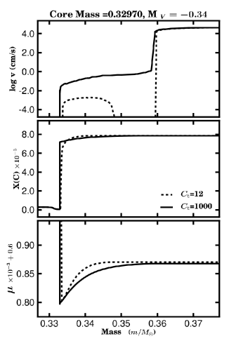
Figure 6: Velocity, $X_{\rm{c}}$ and $\mu$ profiles for the two UKRT models. This is an expanded plot of the first panel in Figure 5 so is once again taken at a hydrogen-exhausted core mass of M_c=0.32970 and $M_{V}=-0.34$ . The C_t=12 model (dashed line) mixes two orders of magnitude more slowly than the C_t=1000 model (solid line). It also fails to transport material to and from the envelope at this stage. It does connect with the envelope before the end of the RGB.

It appears that the requirement for significant carbon depletion is two fold: the position of the minimum in $\mu$ must occur at a reasonably high temperature and we need a sufficiently fast mixing velocity. As a result of our comparison with M3 we prefer the UKRT formalism over that used by EDL08.

6 Constraining the Diffusion Coefficient

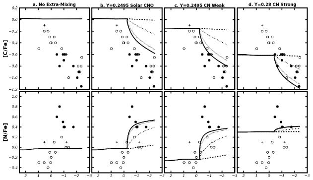
M_V

Figure 7: Carbon and nitrogen abundances as a function of absolute magnitude in M3. Here we compare our models to the Smith (2002) compilation of M3 observations. Open circles denote CN-weak stars, filled circles CN-strong stars, whilst the crosses represent stars of intermediate CN strength. The errors in magnitude are smaller than the symbols used. The maximum error in [C/Fe] and [N/Fe] is $\pm 0.3$ dex. Where extra mixing is included in our models dashed lines correspond to C_t=12 ($\alpha\sim 1$), dot-dashed lines to C_t=120 ($\alpha\sim 2$), dotted lines to C_t=600 ($\alpha\sim 5$) and solid lines to C_t=1000 ($\alpha\sim 2$). Figure 7c includes models with the following initial CNO abundances X(C)=5.45$\times$10^-5, X(N)=1.5$\times$10^-5 and X(O)=2.86$\times$10^-4. In Figure 7d the initial CNO abundances are X(C)=1.9$\times$10^-5, X(N)=5.5$\times$10^-5 and X(O)=2.6$\times$10^-4.

As previously mentioned Kippenhahn et al. (1980), Ulrich (1972) and CZ07a differ in their choice of $\alpha$, the aspect ratio of the fingers by a factor of five and this translates to a difference of two orders of magnitude in C_t. We can also determine a velocity for the mixing through a diffusion equation.

Having selected our preferred formalism we can now use observations to constrain the diffusion coefficient. In Figure 7a we illustrate the effect of standard evolution on the carbon and nitrogen abundances. In all the Figure 7 panels, open circles denote CN-weak stars , filled circles denote CN-strong stars and crosses represent CN-intermediate stars as before. The uncertainty in the data is as specified in Section 5. Figures 7b, 7c and 7d include thermohaline mixing with the UKRT prescription. In each panel we provide four models, these represent different values of C_t. We include: C_t= 12 as per Kippenhahn et al. (1980) (dashed lines, $\alpha\sim 1$), C_t =1000 as per CZ07a (solid lines, $\alpha\sim 6$) and two intermediate values, C_t=120 (dot-dashed lines, $\alpha\sim 2$) and C_t=600 (dotted lines, comparable to Ulrich 1972 C_t=658, $\alpha\sim 5$).

The canonical evolution in Figure 7a shows very little carbon depletion following FDU. This is contrary to the observations for the upper part of the RGB. We include this panel to highlight to the reader the need for extra mixing. In Figure 7b we have assumed a scaled solar CNO abundance and varied the free parameter as described above. It is unlikely that M3 possesses a scaled solar abundance. Russell & Dopita (1992) have already shown that Large Magellanic Cloud abundances are not scaled Solar and we would not expect the environment during globular cluster formation to resemble the solar neighbourhood.

In Figure 7c we have altered the initial CNO abundances whilst keeping the metallicity and total CNO content constant. As the carbon abundance does not change a great deal before the onset of extra mixing we have assumed the most carbon-rich stars are representative of the pre-FDU abundance, similarly for the most nitrogen-poor stars. To match the constraints, the following initial CNO abundances were assumed X(C)=5.45$\times$10^-5, X(N)=1.5$\times$10^-5 and X(O)=2.86$\times$10^-4. We altered the carbon and nitrogen so that we arrived at our desired post-FDU value and adjusted the oxygen abundance in order to keep the total CNO constant. We have decreased the carbon by a factor of 1.47 and the nitrogen by a factor of 1.63 (in relation to solar). These values could easily be fine-tuned to better fit the data but it is the proof of concept we are concerned with. The two slow mixing cases are unable to account for the depletion in carbon. Both C_t=600 and C_t=1000 are a good fit to the carbon and the nitrogen. It does appear that the mixing should begin at a slightly lower luminosity, however Sweigart (1978) demonstrated that lowering the ${}^{4}\mathrm{He}$ abundance will cause the extra mixing to begin earlier because the shell reaches the discontinuity sooner. We find that our models provide a fit to the upper envelope of the run of [C/Fe] vs $M_{V}$ in Figure 7c but can only fit the nitrogen for the CN-weak stars. This argues that much of the spread in [N/Fe] in the lower panels of Figure 4 is dominated by a variation that was present among the cluster stars before they commenced red giant branch evolution. The fact that none of the models in the the lower panels of Figure 4 can reproduce the observed spread in [N/Fe] is suggestive of the CN inhomogeneity in M3 having a predominantly primordial origin. This inference is consistent with the discovery in a number of clusters, including M3 (Norris & Smith, 1984), that N abundance variations (or equivalently CN band strength variations) are found both at and below the magnitude of the bump in the RGB luminosity function (e.g., see Suntzeff & Smith 1991; Briley et al. 2004; Carretta et al. 2005; for the clusters NGC 6752 and M13 which have similar [Fe/H] to M3). This argues strongly for the spread being present in the stars at their birth.

In Figure 7d we have assumed the CN-strong stars are a separate population with their own CNO abundance. Moreover we have assumed there is a CN-[C/Fe] anticorrelation in which the CN-strong stars are initially 0.4 dex depleted in carbon relative to the CN-weak stars (Smith, 2002, and references therein). The CN-strong stars show the results of hot hydrogen burning in the gas from which they formed, including CN and ON cycling. We have therefore changed the initial helium abundance from Y=0.2495 to Y=0.28 as well as the CNO values. Here we set X(C)=1.9$\times$10^-5, X(N)=5.5$\times$10^-5 and X(O)=2.6$\times$10^-4. We find in this case the slower mixing is a good fit for the carbon abundance whilst the faster mixing is able to account for the more extreme observations of carbon depletion. These models are unable to match the more extreme nitrogen enhancements in the CN strong stars. The [N/Fe] is initially so high even on the main sequence that any enhancement due to extra mixing only slightly raises the [N/Fe]. We conclude that much of the nitrogen spread in the CN strong stars is due to primordial variations as a result of hot hydrogen burning (in an early generation of stars that instigated cluster enrichment) rather than thermohaline mixing in the present-day giants.

Our findings are consistent with those of CZ07a in that C_t=1000 is our preferred value of the free parameter in the UKRT thermohaline mixing prescription. In Figure 8 we investigate the effect of increasing C_t beyond 1000. The dotted line corresponds to the EDL08 prescription with $F_{\rm{inv}}$=100, the solid line corresponds to C_t=1000, the dashed line to C_t=3000 ($\alpha\sim$10) and the dotted line C_t=12000 ($\alpha\sim$20). Once again we use the same symbols for the M3 data. The initial abundances are solar scaled CNO, however it is the shape of the profiles we are interested in here. We include the EDL08 model to compare the similarities in the ${}^{3}\mathrm{He}$ depletion as a function of magnitude. The fact that the UKRT ${}^{3}\mathrm{He}$ profiles begin to approach that of the faster mixing EDL08 model once again suggests that depth to which the UKRT models mix is responsible for the carbon depletion. Initially the faster mixing cases are able to deplete the carbon more efficiently than our preferred value of C_t=1000. Although all three values of C_t begin to deplete at different rates they eventually lead to similar levels of CN processing. The similar levels of carbon depletion suggest that a steady state has been reached and for C_t $\geq$ 1000 the process is burning limited.

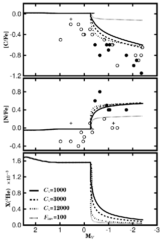
Figure 8: Abundances as function of magnitude. We consider values of C_t beyond 1000. M3 data is represented with the same symbols as in the previous figures. The dotted line corresponds to the EDL prescription with $F_{\rm{inv}}$=100, the solid line corresponds to C_t=1000, the dashed line to C_t=3000 ($\alpha\sim$10) and the dash-dotted line to C_t=12000 ($\alpha\sim$20). There is little difference in the level of carbon depletion once C_t $>$ 1000, because the depletion is limited by the burning rate rather than the transport rate.

7 Mass Loss

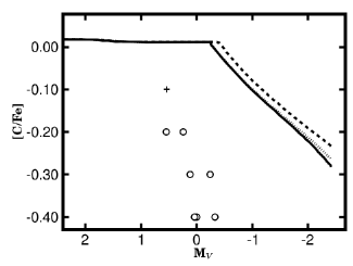
Figure 9: Carbon abundance relative to solar as a function of magnitude. Here we plot UKRT C_t=120 models with varying levels of mass loss. Symbols are described in previous figures. The dashed line corresponds to a model with no mass loss, the dotted line to standard Reimers’ mass-loss rate and the solid curve twice the mass-loss rate. There is little effect on the carbon depletion.

Mass loss could have a significant effect on the level of carbon depletion in the models. If there is less envelope, the amount of carbon that needs to be processed to reduce the [C/Fe] is also less. In Figure 9 we investigate the role of mass loss in the UKRT formula for mixing. We provide three models for the C_t=120 case, standard Reimers’ mass loss (dotted line), no mass loss (dashed line) and a factor of two increase on the standard mass-loss rate (solid line). The effect of mass loss on the surface composition is greatest towards the tip of the giant branch where the mass-loss rate is highest, but even there the alteration in [C/Fe] is slight compared to a zero mass-loss model. These findings are consistent with EDL08, who also find the effect of mass loss negligible after the onset of thermohaline mixing.

8 The Onset of Mixing and the Location of the LF Bump

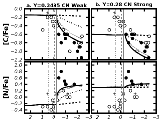
M_V

Figure 10: Carbon and nitrogen abundances as a function of absolute magnitude in M3. These are the same panels as Figures 7c and 7d with the location where the local luminosity maximum occurs when the hydrogen shell meets the composition discontinuity (solid vertical line), the location of the LF bump for M3 from Fusi Pecci et al. (1990) (dashed vertical line) and location of the LF bump for M3 from Smith & Martell (2003) (dot-dashed vertical line).

Our final observational test concerns the onset of mixing and the observed location of the abundance changes. The hydrogen-burning shell will reach the composition discontinuity independent of any thermohaline mixing, which only begins after this event. Once the mixing starts, the rate is dependent on the parameter $C_{t}$ and so the surface abundance begins changing at a visual magnitude that depends slightly on $C_{t}$. The models for the four different values of $C_{t}$ in Figure 7 commence thermohaline mixing within $\Delta M_{V}=0.02$ mag of each other. In Figure 10 we have taken Figures 7c and 7d and marked the position of M3’s LF bump according to (Fusi Pecci et al., 1990, grey dashed line) and the position according to Smith & Martell (2003, dot-dashed grey line). In all four panels we also include the magnitude at which the hydrogen shell reaches the discontinuity in the CN weak models(the solid vertical line). Fusi Pecci et al. (1990) determine the LF bump of M3 to occur at M_V=$-$0.06, Smith & Martell (2003) at M_V=0.45 whereas our models reach the composition discontinuity at M_V=$-$0.26. In the UKRT formula for the diffusion coefficient the change in the surface abundances begins almost immediately after the bump. These results differ somewhat from the non-rotating case of Charbonnel & Lagarde (2010) who find there is a delay of $\sim$ 0.5 magnitudes before the onset of any changes to the surface abundance, albeit for different masses and metallicities to those considered here. The differences between the two quoted values for the LF bump are due to the respective choices of the distance modulus. We find our models are closer to the older results but we refrain from drawing any conclusions. A study that includes lower luminosity giants is required in order for us to make further comparisons to the observations.

In Figure 10b we find that increasing the amount of ${}^{4}\mathrm{He}$ in the model has delayed the onset of the bump. These results are consistent with Sweigart (1978) who in addition to this showed that the size of the discontinuity is also reduced with increasing ${}^{4}\mathrm{He}$ abundance. This is owing to the fact that an increase in ${}^{4}\mathrm{He}$ translates to less hydrogen and less of a discontinuity. The fact that the hydrogen shell encounters the discontinuity later for models with higher initial ${}^{4}\mathrm{He}$ is due to the effect the composition has on the penetration of the convective envelope. A higher hydrogen abundance allows for deeper penetration of the envelope and hence the shell reaches this depth sooner.

9 Conclusion

M3 is a well studied system that demonstrates the abundance patterns we commonly associate with globular clusters. Along with many other clusters it displays significant [C/Fe] depletion along the RGB, the implication being that some form of internal, non-canonical mixing must be occurring. Our models with thermohaline mixing show that the carbon and nitrogen observations can be explained if we adopt the hybrid theory outlined in Smith (2002), where stars in the cluster are undergoing extra mixing as they ascend the RGB and the presence of primordial abundance inhomogeneities due to ON cycling are needed to explain the initial carbon and nitrogen abundances. We have used observations of M3 to investigate our theoretical understanding of thermohaline mixing. Our findings are summarised below:

1. The variation of $\rm{[C/Fe]}$ with magnitude provides a much more stringent test of any proposed extra-mixing mechanism than simply matching the final ${}^{12}\mathrm{C}$/${}^{13}\mathrm{C}$ ratio. When data of sufficient quality is available this can constrain the details of any proposed extra-mixing formulation. In the present case the UKRT formulation of thermohaline mixing is a far better fit than the phenomenological prescription given by EDL08, although both fit the constraint provided by the carbon isotope ratio.

2. The UKRT prescription of thermohaline mixing with C_t=1000 seems to best fit the data for M3. This is consistent with the results of Charbonnel & Lagarde (2010) for higher metallicities and CZ07a for a range of metallicities.

3. We infer that there is a spread of $\sim$0.3 to 0.4 dex in [C/Fe] in the stars in M3 from their birth. Without this initial difference in [C/Fe] between the two populations, thermohaline mixing cannot reproduce the change in [C/Fe] seen on the giant branch. That there are two populations is absolutely required, because once C_t is sufficiently large, an increase of this coefficient doesn’t produce a bigger $\Delta$[C/Fe]. Primordial C and N inhomogeneities have been directly observed as abundance differences among main sequence stars in globular clusters such as M13 and NGC 6752 (Briley et al., 2004; Carretta et al., 2005), which have similar metallicity to M3.

4. Thermohaline mixing can produce the observed values of the carbon isotopes seen in M3.

5. To reproduce the entire spread of [C/Fe] values seen in the giants of M3 it is essential that thermohaline mixing operate in both the CN-strong and CN-weak populations identified in (3). In this case we can explain the full spread in [C/Fe] seen near the tip of the giant branch in M3. A similar exercise was carried out by Denissenkov & VandenBerg (2003) for the case of M92, modelled with a simple parameterized extra-mixing formulation. The data for M92 are from many different sources and make it difficult to estimate precisely where the extra mixing begins. For this reason we do not discuss M92 further in this paper.

6. Thermohaline mixing can produce a significant change in [N/Fe] as a function of M_V on the RGB for initially CN-weak stars but not for initially CN-strong stars, which have so much N to begin with that any extra mixing does not significantly affect the surface composition.

7. The level of depletion of carbon is dependent on the depth to which the material is mixed and how fast it is mixed.

8. Mass loss has little effect on the surface abundances.

9. Both the predicted and observed composition changes take place at a luminosity that is higher than the LF bump in Fusi Pecci et al. (1990). The observed abundances begin to decrease at a luminosity lower than the LF bump preferred by Smith & Martell (2003). Uncertainties in the distance modulus make it difficult to draw further conclusions.

We have seen that the linear theory of Ulrich (1972) and Kippenhahn et al. (1980) provides a fit to the carbon and nitrogen abundances in the giants in M3 (assuming there are two different populations initially). CZ07a have shown that the same theory (and indeed the same parameter C_t=1000) seems to fit field stars of a range of metallicities (see also Charbonnel & Lagarde 2010). It is important to note that thermohaline mixing is more than a theory with an adjustable parameter. For example, its beginning is determined clearly by the fusion of ${}^{3}\mathrm{He}$ which produces a molecular weight inversion. Also, the hydrodynamics provides the physical formulation for the diffusion co-efficient used, and hence its variation throughout the star, to within a constant which depends on the geometry of the fingers expected in the mixing process. Nevertheless, until we have a complete theory that also determines this geometric factor, or at the least some numerical simulations, there is a gap between understanding the fundamental physics and the sort of work presented here, to match the observations. To this end we note the work of Denissenkov (2010) which addresses this issue. There has been recently considerable progress in modelling the oceanic case (Stellmach et al., 2010; Traxler et al., 2010). We are ourselves working on 3D hydrodynamic models in the stellar context, which will be the subject of another paper.

Although our models can explain M3 very well the question remains whether this work can be extended to all clusters. The UKRT prescription for thermohaline mixing appears to model the internal mixing of a young metal rich cluster. Old metal-poor clusters such as M92 will have undergone a different mixing history. Furthermore Sweigart (1978) suggests changing the metallicity and helium content will drastically alter the location and size of the LF bump. Preliminary work by Angelou et al. (2010) will be the subject of subsequent studies. This work further supports the ability of thermohaline mixing to explain extra mixing on the RGB.

10 Acknowledgements

We would like to thank Lionel Siess for helping implement the UKRT mixing by providing us with his matrix solver. We also thank Alessandro Chieffi for providing us with his luminosity to magnitude conversion routine. We extend our gratitude to Christopher Tout for his engaging and helpful discussions on the difference between the two mixing schemes. GCA wishes to thank Matteo Cantiello for his time and subsequent discussions on thermohaline mixing. He also wishes to acknowledge the financial support of the APA scholarship. RPC wishes to acknowledge The Wener Gren Foundation for their financial support. RJS is funded by the Australian Research Council’s Discovery Projects Scheme under grant DP0879472. This work was supported by the NCI National Facility at the ANU.

References

- Abraham & Iben (1970) Abraham Z., Iben Jr. I., 1970, ApJ, 162, L125
- Alves et al. (2004) Alves D. R., Cook K. H., Wishnow E., 2004, in Bulletin of the American Astronomical Society Vol. 36 of Bulletin of the American Astronomical Society, Mass Loss from Red Giants in 2nd-Parameter Globular Clusters: The Ages of M3 and M13. pp 1425–+
- Angelou et al. (2010) Angelou G. C., Lattanzio J. C., Church R. P., Stancliffe R. J., 2010 Observational Constraints for Thermohaline Mixing
- Balser et al. (1997) Balser D. S., Bania T. M., Rood R. T., Wilson T. L., 1997, ApJ, 483, 320
- Balser et al. (2006) Balser D. S., Goss W. M., Bania T. M., Rood R. T., 2006, ApJ, 640, 360
- Balser et al. (1999) Balser D. S., Rood R. T., Bania T. M., 1999, ApJ, 522, L73
- Bellman et al. (2001) Bellman S., Briley M. M., Smith G. H., Claver C. F., 2001, PASP, 113, 326
- Briley et al. (1999) Briley, M. M., Grundahl, F., & Andersen, M. I. 1999, 31, 1369
- Briley et al. (2004) Briley M. M., Cohen J. G., Stetson P. B., 2004, AJ, 127, 1579
- Buonanno et al. (1994) Buonanno R., Corsi C. E., Buzzoni A., Cacciari C., Ferraro F. R., Fusi Pecci F., 1994, A&A, 290, 69
- Busso et al. (2007) Busso M., Wasserburg G. J., Nollett K. M., Calandra A., 2007, ApJ, 671, 802
- Campbell & Lattanzio (2008) Campbell S. W., Lattanzio J. C., 2008, A&A, 490, 769
- Cantiello & Langer (2010) Cantiello, M., & Langer, N. 2010, A&A, 521, A9+
- Carbon et al. (1982) Carbon D. F., Romanishin W., Langer G. E., Butler D., Kemper E., Trefzger C. F., Kraft R. P., Suntzeff N. B., 1982, ApJS, 49, 207
- Carretta et al. (2005) Carretta E., Gratton R. G., Lucatello S., Bragaglia A., Bonifacio P., 2005, A&A, 433, 597
- Cavallo & Nagar (2000) Cavallo R. M., Nagar N. M., 2000, AJ, 120, 1364
- Chaboyer et al. (1992) Chaboyer B., Sarajedini A., Demarque P., 1992, ApJ, 394, 515
- Chanamé et al. (2005) Chanamé, J., Pinsonneault, M., & Terndrup, D. M. 2005, ApJ, 631, 540
- Charbonnel (1994) Charbonnel C., 1994, A&A, 282, 811
- Charbonnel (1995) —. 1995, ApJ, 453, L41+
- Charbonnel (1996) Charbonnel C., 1996, in C. Leitherer, U. Fritze-von-Alvensleben, & J. Huchra ed., From Stars to Galaxies: the Impact of Stellar Physics on Galaxy Evolution Vol. 98 of Astronomical Society of the Pacific Conference Series, Destruction of 3He in Low Mass Stars and Implications for Chemical Evolution. p. 213
- Charbonnel et al. (1998) Charbonnel C., Brown J. A., Wallerstein G., 1998, A&A, 332, 204
- Charbonnel & Do Nascimento (1998) Charbonnel, C., & Do Nascimento, Jr., J. D. 1998, A&A, 336, 915
- Charbonnel & Zahn (2007a) Charbonnel C., Zahn J., 2007a, A&A, 467, L15
- Charbonnel & Zahn (2007b) Charbonnel C., Zahn J., 2007b, A&A, 476, L29
- Charbonnel & Lagarde (2010) Charbonnel, C., & Lagarde, N. 2010, A&A, 522, A10+
- Chen & Han (2004) Chen X., Han Z., 2004, MNRAS, 355, 1182
- Cohen & Meléndez (2005) Cohen J. G., Meléndez J., 2005, AJ, 129, 303
- Dearborn et al. (1975) Dearborn D. S., Bolton A. J. C., Eggleton P. P., 1975, MNRAS, 170, 7P
- Dearborn et al. (2006) Dearborn D. S. P., Lattanzio J. C., Eggleton P. P., 2006, ApJ, 639, 405
- Dearborn et al. (1986) Dearborn D. S. P., Schramm D. N., Steigman G., 1986, ApJ, 302, 35
- Dearborn et al. (1996) Dearborn D. S. P., Steigman G., Tosi M., 1996, ApJ, 465, 887
- Denissenkov (2010) Denissenkov P. A., 2010, ArXiv e-prints
- Denissenkov & Pinsonneault (2008) Denissenkov P. A., Pinsonneault M., 2008, ApJ, 684, 626
- Denissenkov & Tout (2000) Denissenkov P. A., Tout C. A., 2000, MNRAS, 316, 395
- Denissenkov & VandenBerg (2003) Denissenkov, P. A., & VandenBerg, D. A. 2003, ApJ, 593, 509
- Eggleton et al. (2006) Eggleton P. P., Dearborn D. S. P., Lattanzio J. C., 2006, Science, 314, 1580
- Eggleton et al. (2008) Eggleton P. P., Dearborn D. S. P., Lattanzio J. C., 2008, ApJ, 677, 581
- Fusi Pecci et al. (1990) Fusi Pecci F., Ferraro F. R., Crocker D. A., Rood R. T., Buonanno R., 1990, A&A, 238, 95
- Gilroy (1989) Gilroy K. K., 1989, ApJ, 347, 835
- Gilroy & Brown (1991) Gilroy K. K., Brown J. A., 1991, ApJ, 371, 578
- Gratton et al. (2000) Gratton R. G., Sneden C., Carretta E., Bragaglia A., 2000, A&A, 354, 169
- Hata et al. (1995) Hata N., Scherrer R. J., Steigman G., Thomas D., Walker T. P., Bludman S., Langacker P., 1995, Physical Review Letters, 75, 3977
- Hogan (1995) Hogan, C. J. 1995, ApJ, 441, L17
- Iben (1967) Iben, Jr., I. 1967, ApJ, 147, 624
- Jimenez et al. (1996) Jimenez R., Thejll P., Jorgensen U. G., MacDonald J., Pagel B., 1996, MNRAS, 282, 926
- Johnson et al. (2005) Johnson C. I., Kraft R. P., Pilachowski C. A., Sneden C., Ivans I. I., Benman G., 2005, PASP, 117, 1308
- Karakas et al. (2010) Karakas A. I., Campbell S. W., Stancliffe R. J., 2010, ApJ, 713, 374
- Kippenhahn et al. (1980) Kippenhahn R., Ruschenplatt G., Thomas H., 1980, A&A, 91, 175
- Kraft et al. (1992) Kraft R. P., Sneden C., Langer G. E., Prosser C. F., 1992, AJ, 104, 645
- Krishnamurti (2003) Krishnamurti, R. 2003, Journal of Fluid Mechanics, 483, 287
- Laird (1985) Laird J. B., 1985, ApJ, 289, 556
- Lambert & Ries (1977) Lambert D. L., Ries L. M., 1977, ApJ, 217, 508
- Lambert & Ries (1981) Lambert D. L., Ries L. M., 1981, ApJ, 248, 228
- Langer et al. (1986) Langer G. E., Kraft R. P., Carbon D. F., Friel E., Oke J. B., 1986, PASP, 98, 473
- Lee & Cannon (1980) Lee S., Cannon R. D., 1980, Journal of Korean Astronomical Society, 13, 15
- Lind et al. (2009) Lind, K., Primas, F., Charbonnel, C., Grundahl, F., & Asplund, M. 2009, A&A, 503, 545
- Martell et al. (2008) Martell S. L., Smith G. H., Briley M. M., 2008, AJ, 136, 2522
- Mikolaitis et al. (2010) Mikolaitis, Š., Tautvaišienė, G., Gratton, R., Bragaglia, A., & Carretta, E. 2010, MNRAS, 407, 1866
- Newell (1970) Newell E. B., 1970, ApJ, 159, 443
- Nordhaus et al. (2008) Nordhaus J., Busso M., Wasserburg G. J., Blackman E. G., Palmerini S., 2008, ApJ, 684, L29
- Norris & Smith (1984) Norris J., Smith G. H., 1984, ApJ, 287, 255
- Palacios et al. (2006) Palacios A., Charbonnel C., Talon S., Siess L., 2006, A&A, 453, 261
- Palla et al. (2000) Palla, F., Bachiller, R., Stanghellini, L., Tosi, M., & Galli, D. 2000, A&A, 355, 69
- Palmerini et al. (2009) Palmerini S., Busso M., Maiorca E., Guandalini R., 2009, Publications of the Astronomical Society of Australia, 26, 161
- Pavlenko et al. (2003) Pavlenko Y. V., Jones H. R. A., Longmore A. J., 2003, MNRAS, 345, 311
- Pilachowski et al. (2003) Pilachowski C., Sneden C., Freeland E., Casperson J., 2003, AJ, 125, 794
- Piotto (2009) Piotto, G. 2009, 258, 233
- Recio-Blanco & de Laverny (2007) Recio-Blanco A., de Laverny P., 2007, A&A, 461, L13
- Romano et al. (2003) Romano, D., Tosi, M., Matteucci, F., & Chiappini, C. 2003, MNRAS, 346, 295
- Rood et al. (1984) Rood, R. T., Bania, T. M., & Wilson, T. L. 1984, ApJ, 280, 629
- Ruddick & Gargett (2003) Ruddick B., Gargett A., 2003, Progress in Oceanography, 56, 381
- Russell & Dopita (1992) Russell S. C., Dopita M. A., 1992, ApJ, 384, 508
- Sackmann & Boothroyd (1999) Sackmann I., Boothroyd A. I., 1999, ApJ, 510, 217
- Salaris & Weiss (2002) Salaris M., Weiss A., 2002, A&A, 388, 492
- Sandage (1970) Sandage A., 1970, ApJ, 162, 841
- Sandage & Wildey (1967) Sandage A., Wildey R., 1967, ApJ, 150, 469
- Shetrone et al. (2010) Shetrone, M., Martell, S. L., Wilkerson, R., Adams, J., Siegel, M. H., Smith, G. H., & Bond, H. E. 2010, AJ, 140, 1119
- Shetrone (2003) Shetrone M. D., 2003, ApJ, 585, L45
- Smiljanic et al. (2009) Smiljanic R., Gauderon R., North P., Barbuy B., Charbonnel C., Mowlavi N., 2009, A&A, 502, 267
- Smith (2002) Smith G. H., 2002, PASP, 114, 1097
- Smith & Martell (2003) Smith G. H., Martell S. L., 2003, PASP, 115, 1211
- Smith et al. (1996) Smith G. H., Shetrone M. D., Bell R. A., Churchill C. W., Briley M. M., 1996, AJ, 112, 1511
- Sneden et al. (2004) Sneden C., Kraft R. P., Guhathakurta P., Peterson R. C., Fulbright J. P., 2004, AJ, 127, 2162
- Sneden et al. (1986) Sneden C., Pilachowski C. A., Vandenberg D. A., 1986, ApJ, 311, 826
- Stancliffe (2010) Stancliffe R. J., 2010, MNRAS, 403, 505
- Stancliffe et al. (2009) Stancliffe R. J., Church R. P., Angelou G. C., Lattanzio J. C., 2009, MNRAS, 396, 2313
- Stancliffe et al. (2007) Stancliffe R. J., Glebbeek E., Izzard R. G., Pols O. R., 2007, A&A, 464, L57
- Stellmach et al. (2010) Stellmach, S., Traxler, A., Garaud, P., Brummell, N., & Radko, T. 2010, ArXiv e-prints
- Stern (1960) Stern M., 1960, Tellus, 12,172
- Stothers & Simon (1969) Stothers R., Simon N. R., 1969, ApJ, 157, 673
- Suntzeff (1981) Suntzeff N. B., 1981, ApJS, 47, 1
- Suntzeff (1989) Suntzeff N. B., 1989, in G. Cayrel de Strobel ed., The Abundance Spread within Globular Clusters: Spectroscopy of Individual Stars CNO abundances in the metal-poor globular clusters.. pp 71–81
- Suntzeff & Smith (1991) Suntzeff N. B., Smith V. V., 1991, ApJ, 381, 160
- Sweigart (1978) Sweigart A. V., 1978, in A. G. D. Philip & D. S. Hayes ed., The HR Diagram - The 100th Anniversary of Henry Norris Russell Vol. 80 of IAU Symposium, Survey of some recent stellar-evolution calculations. pp 333–343
- Sweigart & Mengel (1979) Sweigart A. V., Mengel J. G., 1979, ApJ, 229, 624
- Tomkin et al. (1976) Tomkin J., Luck R. E., Lambert D. L., 1976, ApJ, 210, 694
- Tosi (1998) Tosi, M. 1998, Space Sci. Rev., 84, 207
- Traxler et al. (2010) Traxler, A., Stellmach, S., Garaud, P., Radko, T., & Brummell, N. 2010, ArXiv e-prints
- Trefzger et al. (1983) Trefzger D. V., Langer G. E., Carbon D. F., Suntzeff N. B., Kraft R. P., 1983, ApJ, 266, 144
- Ulrich (1971) Ulrich R. K., 1971, ApJ, 168, 57
- Ulrich (1972) Ulrich R. K., 1972, ApJ, 172, 165
- VandenBerg (2000) VandenBerg D. A., 2000, ApJS, 129, 315
- Weiss & Charbonnel (2004) Weiss A., Charbonnel C., 2004, Memorie della Societa Astronomica Italiana, 75, 347