High Jet Efficiency and Simulations of Black Hole Magnetospheres

Abstract

This article reports on a growing body of observational evidence that many powerful lobe dominated (FR II) radio sources likely have jets with high efficiency. This study extends the maximum efficiency line (jet power $\approx$ 25 times the thermal luminosity) defined in Fernandes et (2010) so as to span four decades of jet power. The fact that this line extends over the full span of FR II radio power is a strong indication that this is a fundamental property of jet production that is independent of accretion power. This is a valuable constraint for theorists. For example, the currently popular ”no net flux” numerical models of black hole accretion produce jets that are 2 to 3 orders of magnitude too weak to be consistent with sources near maximum efficiency.

1 Introduction

Relativistic jets emanating from AGN (active galactic nuclei) exist in a variety of strengths. Most quasars are radio quiet objects that have either no measurable jets or jets that are so weak that they often cannot propagate out of the host galaxy. About $\gtrsim 10\%$ of AGN have highly luminous radio jets of which $\approx 20\%$ are classic FR II radio sources defined by jets that propagate hundreds of kpc, terminating in lobes of plasma with similar linear extent (deVries et al., 2006). The energy flux in these jets, $Q$, can be enormous with many independent estimates finding long term time averages, $\overline{Q}\gtrsim 10^{47}\mathrm{ergs/sec}$ (Willott et al., 1999; Punsly, 2007c). These jets are not perfectly steady, so there are episodes in which the instantaneous power, $Q(t)$, must be even larger. In this Letter, an attempt is made to expand on and consolidate the evidence for large jet power that has been accumulating in the literature since 2006.

The second section quantifies $Q$ relative to the dynamics of the accreting gas. From observations, one can estimate the ratio of $Q$ to the thermal luminosity of the accretion flow, $L_{bol}$, defined as $R\equiv Q/L_{bol}$ or with respect to the mass accretion rate $Q\equiv\eta_{Q}\dot{M}c^{2}$, where $\eta$ is called the efficiency. Strong radio sources can be described in terms of a concept of maximum jet efficiency that was introduced by Fernandes et al (2010), i.e a maximum value of $R$ or $\eta_{Q}$ for radio jets. The maximum jet efficiencies implied by various lines of research are compiled. The results are analyzed for consistency and are critically examined in terms of the assumptions and limitations of each method.

In the third section, we discuss the high efficiency sources from section 2 in the context of current numerical work, the 3-D numerical simulations of MHD (magnetohydrodynamic) accretion flows around black holes with no net magnetic flux. The nexus between these simulations and observation is that the simulated $Q$ is always expressible in units of $\dot{M}c^{2}$ by all research groups. By making reasonable assumptions about $\eta_{th}$, the thermal efficiency ($L_{bol}=\eta_{th}\dot{M}c^{2}$), as derived by accretion disk theory and new turbulent MHD simulations, one can compare the observations with the simulations.

2 Evidence for High Jet Efficiency

Ever since the seminal work of Rawlings and Sanders (1991), astrophysicists have been trying to estimate the enormous energy flux that feeds the radio lobes in FR II radio sources and relate it to the thermal luminosity of the accretion flow. The three most viable options for estimating $Q$ are either based on the low frequency (151 MHz) flux from the radio lobes on 100 kpc scales (eg. Willott et al. (1999)), or the work done creating the cavities that are carved out of the intra-cluster medium by the expanding radio lobes (eg. Birzan et al (2004); McNamara et al (2010)), or models of the broadband Doppler boosted synchrotron and inverse Compton radiation spectra associated with the relativistic parsec scale jet (eg. Ghisellini et al (2010)). Each method has its advantage. The 151 MHz method is the most widely applicable, all that is needed is a radio spectrum. A disadvantage is that it involves long term time averages, $\overline{Q}$, that do not necessarily reflect the current state of quasar activity. The second method is also not contemporaneous, yet more accurate in principle than the first, but is restricted to low redshift sources with deep X-ray observations. The last method is contemporaneous, so one can define a directly interpretable ratio of jet to accretion thermal power, $R(t)=Q(t)/L_{bol}$. However, one is forced to deal with estimating the large Doppler enhancement factor, $\delta$, which is a potential source of large uncertainty (the jet luminosity scales like $\delta^{4}$). In this section, using these three methods, we expand on the notion of a maximum jet efficiency defined in Fernandes et al (2010) that is based on 151 MHz flux estimate.

In Figure 1, the black squares are a scatter plot, $\overline{Q}$ versus $L_{bol}$, of the complete sample of FRII narrow line radio galaxies (NLRGs) from Fernandes et al (2010). The low frequency selected sample is limited to $0.9<z<1.1$, as a compromise between having sufficient cosmic volume to find strong radio sources and being sufficiently close so that these sources can be detected in the IR. $L_{bol}=8.5\nu L_{\nu}(12\mu\mathrm{m})$ is computed from the IR luminosity at 12 $\mu\mathrm{m}$ Richards et al (2006). They define a diagonal line at $\overline{R}\equiv\overline{Q}/L_{bol}=25$ (the black solid line in Figure 1), the maximum efficiency line. The dashed blue vertical line represents the approximate dividing line between Seyfert 1 galaxy and quasar luminosity ($M_{V}=-23$). The dashed vertical orange line represents the dividing line between solely Seyfert 1 galaxies and a mixture of LLAGNs (low luminosity AGN) and weaker Seyfert 1 galaxies (Ho, 2005). In contrast to Seyfert 1 galaxies and quasars, the LLAGNs do not have a strong ”blue bump” in their spectra, the signature of strong thermal emission from an accretion flow (Ho, 2005; Sun and Malkan, 1989). The LLAGNs are estimated to have inefficient modes of accretion, expressed in terms of the Eddington luminosity as $L_{bol}/L_{Edd}<10^{-5}$ in contrast to quasars and Seyfert galaxies which typically have $10^{-2}<L_{bol}/L_{Edd}<1$ (Ho, 2005; Sun and Malkan, 1989). Thus, Figure 1 indicates that the NLRGs in the Fernandes et al (2010) sample are likely to have a central black hole in a high efficiency accretion state typical of a quasar or Seyfert 1 galaxy, but the optical/UV core is hidden.

Figure 1: The maximum efficiency line is illustrated in this scatter plot of $Q$ and $L_{bol}$. The scatter plot shows that $1<R<25$ is not an unusual state of jet activity.

One can expand the Fernandes et al (2010) treatment to a larger range of black hole accretion states and jet power, by considering the low redshift sample of IR observations of FRII NLRGs of Ogle et al (2006). The same IR bolometric correction and $\overline{Q}$ estimators can be used as in Fernandes et al (2010). They noticed a diagonal boundary in a scatter plot of IR luminosity versus 178 MHz flux which is similar to the maximum efficiency line. In Figure 1, the orange circles represent these ”weak Mid-IR sources” from Ogle et al (2006). Notice how well the orange circles respect the maximum efficiency line. The trend now extends below the upper limit of LLAGN luminosity. Since Seyfert 1 galaxies also exist at such luminosity, and the trend looks smooth, there does not seem to be any evidence of a change in accretion mode for FRII NLRGs at $L_{bol}<6\times 10^{43}$ ergs/sec.

A small sample of FRII NLRGs from McNamara et al (2010) is also plotted as blue triangles in Figure 1. In this sample, $\overline{Q}$ is estimated by an independent method, the work done to create large bubbles in the intra-cluster medium. The IR luminosity is estimated from the data in Shi et al (2005) with the synchrotron component subtracted off and the IR bolometric correction is from Richards et al (2006). This data also conforms with the maximum efficiency line concept.

Another method of quantifying a jet as highly efficient is to choose sources with $\overline{Q_{Edd}}=\overline{Q}/L_{Edd}>1$. This is an extreme condition since $L_{bol}/L_{Edd}>1$ quasars are either extremely rare or as is often argued nonexistent (Marconi et al, 2009; Netzer, 2009). Thus, the $\overline{Q_{Edd}}$ sources would almost certainly have instantaneous episodes with $R(t)>1$. A small sample of these sources were found in Punsly (2007c). These are the red diamonds in Figure 1 and overlap the high end of the Fernandes et al (2010) scatter. They are lobe dominated quasars for which UV continuum emission and broad line strengths were used to estimate $L_{bol}$ and 151 MHz flux was used to estimate $\overline{Q}$. Note that the Fernandes et al (2010) and the Punsly (2007c) samples are consistent with a maximum value of $\overline{Q}\gtrsim 10^{47}$ ergs/sec that seems to make the maximum efficiency line bend over towards the equipartition line defined by $R=1$.

The fact that $\overline{Q}$ seems to reach a maximum does not necessarily mean that there are not even larger instantaneous jet powers. By fitting broadband blazar spectra, from the radio band to gamma rays, Ghisellini et al (2010) believe that they have a method to extract the jet power within a few light years of the central black hole in a blazar - almost contemporaneous on cosmic time scales. The model is one of a highly relativistic magnetized plasmoid propagating in the radiation environment of the quasar. The inverse Compton emission is necessarily modeled simultaneously with an accretion disk model of the ”big blue bump” for each source. The method is a bit controversial because of the large Doppler enhancement in blazar jets and the uncertainty that it introduces in the intrinsic luminosity. The appeal of this method is that it is completely independent of the techniques used for the other data in Figure 1. In order not to clutter Figure 1, only the $R(t)>2$ blazars are plotted. These $Q(t)$ estimates (that are plotted as dark blue circles) also respect the maximum efficiency line with only two outliers.

None of the methods used to create the data sets in Figure 1 is a rigorous justification of the maximum efficiency line in isolation. However, the agreement that is achieved by these independent experiments are strong scientific evidence in support of the notion of the maximum efficiency line found in Fernandes et al (2010) that is now extended to over 4 decades in $Q$. The fact that this line extends over the full span of FR II radio power is an indication that this is a fundamental property of jet production that is independent of accretion power. Another important aspect of Figure 1 is that powerful FR II radio sources are plentiful in the range $1<R<25$. Furthermore, since jet power is not steady over the lifetime of the QSO, many of the sources below the $R=1$ line likely have episodes in the high efficiency range $1<R<25$, i.e. this is not an aberrant or outlier state of jet activity.

Figure 2: A comparison of 3-D numerically simulated data with the constraints on jet power in terms of accretion rate ($Q/\dot{M}c^{2}$) imposed by observations. The ”region of high jet efficiency” corresponds to the region between $R=1$ and $R=25$ in Figure 1.

3 Theoretical Discussion

In the past, we were forced to compare a scatter plot like Figure 1 to theory by means of parametric models. However, these models have a large unknown, the strength of the magnetic field (Blandford and Znajek, 1977; Meier, 2001; Nemmen et al, 2007). The ability of a turbulent accretion disk to transport and sustain large scale magnetic flux is controversial, rendering the flux distribution as a major unknown (Ghosh and Abramowicz, 1997; Livio et al, 1999; Rothstein and Lovelace, 2008; Reynolds et al, 2006). Long term MHD simulations in a generally relativistic background can at least provide a self-consistent magnetic field distribution (be it not necessarily unique). Thus, the best tools that we have to investigate the central engine of radio loud AGN, without the over-riding uncertainty of the field distribution, are the current battery of long term 3-D numerical simulations of black hole accretion systems (McKinney and Blandford, 2009; Beckwith et al, 2008b; Hawley and Krolik, 2006; Krolik et al, 2005; Fragile et al, 2007). The initial state is a thick torus of gas in equilibrium that is threaded by concentric loops of weak magnetic flux that foliate the surfaces of constant pressure. There is no net magnetic flux in these simulations. If the loops are configured in the same orientation and are poloidal and not toroidal then the leading edge that accretes will deposit a net poloidal flux on the black hole and a jet forms (Beckwith et al, 2008b). In these simulations, $Q$ is expressible in terms of accretion rate onto the black hole, $\dot{M}c^{2}$. Thus, one can compare different simulations and one can compare to the observations if $\eta_{th}$ is known. Theoretically, $\eta_{th}$ was determined by Novikov and Thorne (1973). This was recently questioned since the boundary condition of zero stress at the inner most stable orbit was suspect (Gammie, 1999; Krolik et al, 1999). In spite of this, recent high resolution simulations of accretion disks indicate that the Novikov and Thorne (1973) value is accurate to within a few percent for thin disks and only increases modestly for high spin rates (expressed as $a/M\lesssim 1$, where ”M” and ”a” are the black hole mass and specific angular momentum, respectively) and thick disks (Beckwith et al, 2008a; Penna et al, 2010; Noble and Krolik, 2009). Therefore, in the context of this discussion, the Novikov and Thorne (1973) value of $\eta_{th}$ is suitable for the purpose of comparing the simulations to the maximum efficiency line in Figure 2. Recall that the sources in Figure 1 have $L_{bol}$ consistent with large viscous dissipation (big blue bump), so a thermally luminous disk model is appropriate as opposed to low efficiency advection dominated accretion (Narayan and Yi, 1995).

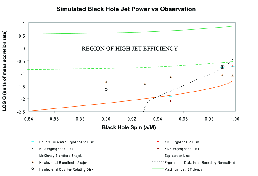
Figure 2 compares the 3-D simulated data to the maximum efficiency line. The McKinney and Blandford (2009) a/M=0.92 simulation shows a Blandford-Znajek (B-Z) jet as in Blandford and Znajek (1977). They note that $Q\approx 0.01\dot{M}c^{2}$ is similar to the 2-D solutions reported in McKinney (2005). Thus, the spin dependent efficiency equation, equation (3) of McKinney (2005) is plotted above. The other B-Z jet data (collectively referred to as Hawley et al. Blandford-Znajek in Figure 2) comes from Hawley and Krolik (2006); Krolik et al (2005) except for the a/M = 0.99 and the a/M=0.998 data. The reason for the new data points is that the high spin cases a/M=0.998 (KDE) form Krolik et al (2005); Punsly (2006) and a/M=0.99 (KDJ) from Hawley and Krolik (2006); Punsly (2007a); Punsly et al (2010) have a strong ergospheric disk jet (as indicated in the Figure2) that suppresses the B-Z jet (Punsly, 2007b). To find the power of a pure B-Z jet, the raw data from two simulations (that were used for ray tracing in Beckwith et al (2008a)) that was generously provided to this author by John Hawley, KDEb (a/M=0.998) and KDJd (a/M=0.99), was reduced. These simulations were different from KDE and KDJ because the code was modified to include artificial diffusion terms in the equations of continuity, energy conservation, and momentum conservation as described in De Villiers (2006). The resultant numerical diffusion suppressed the ergospheric disk jet giving a more pristine estimate of the B-Z efficiency than can be obtained from KDE and KDJ. The simulation, KDH (a/M=0.95), has a weak ergospheric disk jet so the estimates for the B-Z power are straightforward Punsly (2007b). The mechanical energy flux is included in these estimates which can be non-negligible in some of the high spin simulations (Punsly, 2007b). Note that no accretion disk jets form in any of these simulations.

Notice that all the no net flux simulations in Figure 2 fall below the region of high jet efficiency, $1<R<25$ from Figure 1, being 2 to 3 orders of magnitude less efficient than the most efficient jets. The only simulations that are close are the high spin ergospheric disk jets from KDE and KDJ. But they are still just below the region of high jet efficiency. Can the a/M=0.998 case be optimized to reproduce the high jet efficiency? To answer this, we explore the curious situation that the ergospheric disk jet in KDE is not much stronger than KDJ contrary to the theory (Punsly, 2008). A spin dependent expression for the ergospheric disk jet Poynting flux (approximately $Q$ in this discussion), $S$, can be approximated as

$$S\approx N(B^{2})\left[[SA]\Omega_{H}\right]^{2}\;,$$ (1)

where the vertical magnetic field in the ergospheric disk is $B$, the surface area of the ergospheric disk is $SA$ and the field line angular velocity scales with the horizon angular velocity, $\Omega_{H}$, and $N(B^{2})$ is a normalization constant (Punsly, 2008). The theory does not fix the distribution on $B$ in time and space and $SA$ of the jet producing region that will occur in a given numerical simulation. In equation (1), the empirical distribution of $B^{2}$ is absorbed in the normalization constant $N$. In principle, $SA$ of the equatorial plane in the ergosphere, changes very rapidly with spin for $a/M\lesssim 1$, hence the expectation of significantly larger jet power for KDE than for KDJ (Punsly, 2008). Setting $N=0.0028$ in equation (1) creates the ”doubly truncated ergospheric disk,” a two parameter ($SA$ and $\Omega_{H}$) fit to the simulated data in Figure 2. It is doubly truncated because the jet does not fill the entire ergospheric equatorial plane, but is restricted to the region $r_{in}<r<1.50M$, where $r_{in}$ is the inner calculational boundary (located outside the event horizon, $r_{in}>r_{H}$). For some unknown reason, the vertical flux that creates the jet dies off rapidly beyond $r=1.50M$ in the simulations. Yet, in principle, an ergospheric disk can exist throughout the ergosphere $r_{H}<r<2M$ (Punsly, 2008). The simple two parameter equation (1) (with $N$ fixed) is a reasonable fit to the numerical data (the 3 blue dashes in Figure 2) and explains the dependence of $S$ on $a$. Equation (1) implies that the reason KDE is not much stronger than KDJ is because $SA$ in the computational grids of the two simulations is virtually identical ($\approx 18M^{2}$ in geometrized units). If one were to move $r_{in}$ in KDE inward so that it is normalized to the the KDJ scaling of $r_{in}(KDJ)=1.203M=1.054r_{H}$, one expects a larger $SA$ and therefore a larger jet power, (i.e. change the inner calculational boundary in the numerical grid of KDE from $r_{in}(KDE)=1.175M$ to $r_{in}=1.054r_{H}=1.12M$). $SA$ is increased to $23.3M^{2}$ for a/M=0.998 if $r_{in}=1.12M<r<1.5M$. The black dashed curve in Figure 2 is a plot of the predicted $S$ from equation (1) with the empirically fit value of $N=0.0028$ from the simulated data and normalized numerical grids defined by $r_{in}=1.054r_{H}$. Even with the enhancement in power for a/M = 0.998, with a renormalized grid, the curve barely penetrates the region of high jet efficiency. Based on this analysis of this most efficiently known simulated jet, it is concluded that any attempt to optimize the no net flux scenario will still be too weak to explain the region of high jet efficiency in Figure 2.

4 Conclusion

This study shows that the maximum jet efficiency condition, $R\approx 25$, extends over the entire range of known FR II jet powers. It is demonstrated that the no net flux accretion numerical models can not explain the large number of high efficiency jets with $R>1$. Furthermore, the initial no net flux state in the considered simulations is configured to yield the maximum jet power. The situation for no net flux is even more nonconforming if the initial field is not composed of loops of the same vertical orientation, but randomly oriented. In this case, the jet power can be reduced by three orders of magnitude or more (Beckwith et al, 2008b). It is concluded that the no net flux models are not suitable numerical models for powerful radio loud quasars. Clearly some other dynamical element is needed in the setup of the simulations. Perhaps it is the accretion of a large reservoir of large scale magnetic flux as in Igumenshchev (2008). This can have two relevant effects. First, the ergospheric disk power should be greatly increased (Punsly et al, 2010). Also, unlike the no net flux simulations, a magnetized accretion disk forms in Igumenshchev (2008).

Finally, note that Figure 2 does not indicate that large ”a” acts likes a switch that transforms a radio quiet black hole accretion system into one with high jet efficiency. The only thing that looks remotely like a switch in Figure 2 is the ergospheric disk. This conclusion is in accord with the B-Z switch model of Tchekhovskoy et al (2010) that requires radio quiet (loud) quasars to have spins $a\approx 0.15$ ($a\approx 1$). This scenario seems unlikely, radio quiet quasars are typically selected by optical/UV luminosity and therefore should have elevated (mass and angular momentum) accretion rates and large $a$ (Bardeen, 1970). The magnetospheres in Tchekhovskoy et al (2010) are shaped by a boundary condition. There is no accretion in the simulation, therefore there is no calibrated measure of the jet strength with respect to $\dot{M}c^{2}$.

References

- Bardeen (1970) Bardeen, J. 1970 Nature 226 64
- Beckwith et al (2008a) Beckwith, K., Hawley, J., Krolik, J. 2008, MNRAS 390 21
- Beckwith et al (2008b) Beckwith, K., Hawley, J., Krolik, J. 2008, ApJ 678 1180
- Birzan et al (2004) Birzan, L. et al 2004, ApJ 607 800
- Blandford and Znajek (1977) Blandford, R. and Znajek, R. 1977, MNRAS. 179, 433
- De Villiers (2006) De Villiers, J-P. 2006, astro-ph/0605744
- deVries et al. (2006) deVries, W., Becker, R., White, R. 2006, AJ 131 666
- Fernandes et al (2010) Fernandes, C. 2010, MNRAS in press arXiv:1010.0691v1
- Fragile et al (2007) Fragile, P. C., Blaes, O. M., Anninos, P., Salmonson, J. D. 2007, ApJ 668 417
- Gammie (1999) Gammie, C. 1999 ApJL 522 575
- Ghisellini et al (2010) Ghisellini, G. et al 2010, MNRAS 405, 387
- Ghosh and Abramowicz (1997) Ghosh, P., & Abramowicz, M. A. 1997, MNRAS 292, 887
- Hawley and Krolik (2006) Hawley, J., Krolik, K. 2006, ApJ 641 103
- Ho (2005) Ho, L. 2005 In: From X-ray Binaries to Quasars: Black Hole Accretion on All Mass Scales ed. by Maccarone,T., Fender,R. and Ho, L.C. (Dordrecht: Kluwer) p.219 astro-ph/0504643
- Igumenshchev (2008) Igumenshchev, I. V. 2008, ApJ 677 317
- Krolik et al (1999) Krolik, J. 1999 ApJL 515 73
- Krolik et al (2005) Krolik, J., Hawley, J., Hirose, S.2005, ApJ 622, 1008
- Laing et al (1983) Laing, R. Riley, J. and Longair, M. 1983, MNRAS 204, 151
- Livio et al (1999) Livio, M., Ogilvie, G. and Pringle, J. 1999, ApJ 512, 100
- Marconi et al (2009) Marconi, A. et al 2009, ApJL 698 103
- McKinney (2005) McKinney, J. 2004, ApJL630 5
- McKinney and Blandford (2009) McKinney, J., Blandford, R. 2009, MNRAS Letters 394 126
- McNamara et al (2010) McNamara, B., Rohanizadegan, M., Nulsen, P. 2010, accepted by ApJ arXiv:1007.1227
- Meier (2001) Meier, D. L. 2001, ApJL 548 9
- Narayan and Yi (1995) R. Narayan, I. Yi 1995 ApJ 452,710
- Nemmen et al (2007) Nemmen, R.,Bower, R., Babul, A., Storchi-Bergmann, T. 2007, MNRAS 3771652
- Netzer (2009) Netzer, H. 2009 ApJ 695 793
- Noble and Krolik (2009) Noble, S., Krolik, J. 2009, ApJ 692, 411
- Novikov and Thorne (1973) Novikov, I. and Thorne, K. 1973, in Black Holes: Les Astres Occlus, eds. C. de Witt and B. de Witt (Gordon and Breach, New York), 344
- Ogle et al (2006) Ogle, P., Whysong, D. and Antonucci, R.2006 ApJ 647 161
- Penna et al (2010) Penna, R. et al 2010, MNRAS 377 1652
- Punsly (2008) Punsly, B. 2008, Black Hole Gravitohydromagnetics, second edition (Springer-Verlag, New York)
- Punsly (2007a) Punsly, B. 2007a, ApJL 661, 21
- Punsly (2007b) Punsly, B. 2007b, MNRAS Letters 381,79
- Punsly (2007c) Punsly, B. 2007c, MNRAS 374 10
- Punsly (2006) Punsly, B. 2006, MNRAS 366 29
- Punsly et al (2010) Punsly, B., Igumenshchev, I. V., Hirose, S. 2010, ApJ 704, 1065
- Rawlings et al. (2001) Eales, S. Rawlings, S., Eales, S. and Lacy, M. 1997, MRAS 322 523
- Rawlings and Sanders (1991) Rawlings, S. and Saunders, 1991, Nature 349 138
- Reynolds et al (2006) Reynolds,C., Garofalo, D.and Begelman, M. 2006, ApJ 651 1023
- Richards et al (2006) Richards, G. et al 2006, ApJS 166 470
- Rothstein and Lovelace (2008) Rothstein, D. and Lovelace, R. V. E. 2008, ApJ 677 1221
- Shi et al (2005) Shi, Y. et al 2005, ApJ 629 88
- Sun and Malkan (1989) Sun, W.H., Malkan, M. 1989, ApJ 346 68
- Tchekhovskoy et al (2010) Tchekhovskoy, A., Narayan, R. and McKinney, J. 2010, ApJ 711 50
- Willott et al. (1999) Willott, C., Rawlings, S., Blundell, K., Lacy, M. 1999, MNRAS 309 1017