Smoothed Particle Hydrodynamics and Magnetohydrodynamics

Abstract

This paper presents an overview and introduction to Smoothed Particle Hydrodynamics and Magnetohydrodynamics in theory and in practice. Firstly, we give a basic grounding in the fundamentals of SPH, showing how the equations of motion and energy can be self-consistently derived from the density estimate. We then show how to interpret these equations using the basic SPH interpolation formulae and highlight the subtle difference in approach between SPH and other particle methods. In doing so, we also critique several ‘urban myths’ regarding SPH, in particular the idea that one can simply increase the ‘neighbour number’ more slowly than the total number of particles in order to obtain convergence. We also discuss the origin of numerical instabilities such as the pairing and tensile instabilities. Finally, we give practical advice on how to resolve three of the main issues with SPMHD: removing the tensile instability, formulating dissipative terms for MHD shocks and enforcing the divergence constraint on the particles, and we give the current status of developments in this area. Accompanying the paper is the first public release of the ndspmhd SPH code, a 1, 2 and 3 dimensional code designed as a testbed for SPH/SPMHD algorithms that can be used to test many of the ideas and used to run all of the numerical examples contained in the paper.

url]http://users.monash.edu.au/$\sim$dprice/SPH/

1 Introduction

Smoothed Particle Hydrodynamics (SPH), originally formulated by Lucy (1977) and Gingold and Monaghan (1977), is by now very widely used for many diverse applications in astrophysics, geophysics, engineering and in the film and computer games industry. Whilst numerous excellent reviews already exist (e.g. Monaghan, 1992, 2005; Price, 2004; Rosswog, 2009), there remain – particularly in the astrophysical domain – some widespread misconceptions about its use, and more importantly, its fundamental basis.

Our aim in this – mainly pedagogical – review is therefore not to provide a comprehensive survey of SPH applications, nor the implementation of particular physical models, but to re-address the fundamentals about why and how the method works, and to give practical guidance on how to formulate general SPH algorithms and avoid some of the common pitfalls in using SPH. Since such an understanding is critical to the development of robust and accurate methods for Magnetohydrodynamics (MHD) in SPH (hereafter referred to as “Smoothed Particle Magnetohydrodynamics”, SPMHD), this will lead us naturally on to review the background and current status in this area – particularly relevant given the importance of MHD in most, if not all, astrophysical problems. Whilst the paper is written with an astrophysical flavour in mind (given the topical issue of JCP for which it is written), the principles are general and thus are applicable in any of the areas in which SPH is applied.

Finally, alongside this article I have released a public version of my ndspmhd SPH/SPMHD code, along with a set of easy-to-follow numerical exercises – consisting of setup and input files for the code and step-by-step instructions for each problem in 1, 2 and 3 dimensions – the problems themselves having been chosen to illustrate many of the theoretical points in this paper. Indeed, ndspmhd has been used to compute all of the test problems and examples shown. The hope is that this will become a useful resource not only for advanced researchers but also for students embarking on an SPH-based research topic.

2 The foundations of SPH: Calculating density

The usual introductory lines on SPH refer to it as a “Lagrangian particle method for solving the equations of hydrodynamics”. However, SPH starts with a basis much more fundamental than that, as the answer to the following question:

How does one compute the density from an arbitrary distribution of point mass particles?

This problem arises in many areas other than hydrodynamics, for example in obtaining the solution to Poisson’s equation for the gravitational field $\nabla^{2}\Phi=4\pi G\rho({\bf r})$ when a (continuous) density field is represented by a collection of point masses.

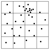
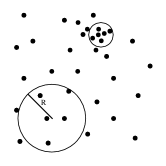
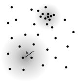
Figure 1: Computing a continuous density field from a collection of point mass particles. a) In particle-mesh methods (left panel) the density is computed by interpolating the mass to a grid (or simply dividing the mass by the volume). However, this tends to over/under resolve clustered/sparse regions. b) An alternative not requiring a mesh is to construct a local volume around the sampling point, solving the clustering problem by scaling the sample volume according to the local number density of particles. c) This panel shows the approach adopted in SPH, where the density is computed via a weighted sum over neighbouring particles, with the weight decreasing with distance from the sample point according to a scale factor $h$.

2.1 Approaches to computing the density

Three common approaches are summarised in Fig. 1. Perhaps the most straightforward (Fig. 1a) is to construct a mesh of some sort and divide the mass in each cell by the volume. This basic approach forms the basis of hybrid particle-mesh methods such as Marker-In-Cell (e.g. Harlow and Welch, 1965) and Particle-In-Cell (Hockney and Eastwood, 1981) schemes, where one can further improve the density estimate using any of the standard particle-cell interpolation methods, such as Cloud-In-Cell (CIC), Triangular-Shaped-Cloud (TSC) etc. However there are clear limitations – firstly that a fixed mesh will inevitably over/under-sample dense/sparse regions (respectively) when the mass distribution is highly clustered; and secondly a loss of accuracy, speed and consistency because of the need to interpolate both to/from the particles, for example to compute forces.

The second approach (Fig. 1b) is to remove the mesh entirely and instead calculate the density based on a local sampling of the mass distribution, for example in a sphere centred on the location of the sampling point (which may or may not be the location of a particle itself). The most basic scheme would be to divide the total mass by the sampling volume, i.e.,

$$\rho({\bf r})=\frac{\sum_{b=1}^{N_{neigh}}m_{b}}{\frac{4}{3}\pi R^{3}}.$$ (1)

The problem of resolving clustered/sparse regions can be easily addressed in this method by adjusting the size of the sampling volume according to the local number density of sampling points, for example by computing with a fixed “number of neighbours” for each particle – as shown in the Figure. However, this leads to a very noisy estimate, since the density estimate will be very sensitive to whether a distant particle on the edge of the volume is “in” or “out” of the estimate (with $\delta\rho\propto 1/N_{neigh}$ for equal mass particles). This leads naturally to the idea that one should progressively down-weight the contributions from neighbouring particles as their relative distance increases, in order that changes in distant particles have a progressively smaller influence on the local estimate (that is, the density estimate is smoothed).

2.2 The SPH density estimator

This third approach forms the basis of SPH and is shown in Fig. 1c: Here the density is computed using a weighted summation over nearby particles, given by

$$\rho({\bf r})=\sum_{b=1}^{N_{neigh}}m_{b}W({\bf r}-{\bf r}_{b},h),$$ (2)

where $W$ is an (as yet unspecified) weight function with dimensions of inverse volume and $h$ is a scale parameter determining the rate of fall-off of $W$ as a function of the particle spacing (also yet to be determined). Conservation of total mass $\int\rho{\rm dV}=\sum_{b=1}^{N_{part}}m_{b}$ implies a normalisation condition on $W$ given by

$$\int_{\rm V}W({\bf r}^{\prime}-{\bf r}_{b},h){\rm dV^{\prime}}=1.$$ (3)

The accuracy of the density estimate then rests on the choice of a sufficiently good weight function (hereafter referred to as the smoothing kernel). Elementary considerations suggest that a good density kernel should have at least the following properties:

1. A weighting that is positive, decreases monotonically with relative distance and has smooth derivatives;

2. Symmetry with respect to (${\bf r}-{\bf r}^{\prime}$) – i.e., $W({\bf r}^{\prime}-{\bf r},h)\equiv W(|{\bf r}^{\prime}-{\bf r}|,h)$; and

3. A flat central portion so the density estimate is not strongly affected by a small change in position of a near neighbour.

A natural choice that satisfies all of the above properties is the Gaussian:

$$W({\bf r}-{\bf r}^{\prime},h)=\frac{\sigma}{h^{d}}\exp\left[-\frac{({\bf r}-{\bf r}^{\prime})^{2}}{h^{2}}\right],$$ (4)

where $d$ refers to the number of spatial dimensions and $\sigma$ is a normalisation factor given by $\sigma=[1/\sqrt{\pi},1/\pi,1/(\pi\sqrt{\pi})]$ in [1,2,3] dimensions. The Gaussian satisfies condition 1 particularly well since it is infinitely smooth (differentiable) – and gives in practice an excellent density estimate. However it has the practical disadvantage of requiring interaction with all of the particles in the domain [with computational cost of $\mathcal{O}(N^{2})$ if computing the density at the particle locations], despite the fact that the relative contribution from neighbouring particles quickly becomes negligible with increasing distance. Thus in practice it is better to use a kernel that is Gaussian-like in shape but truncated at a finite radius (e.g. a few times the scale length, $h$). Using kernels with such “compact support” means a much more efficient density evaluation, since the cost scales like $\mathcal{O}(N_{neigh}N)$, but inevitably leads to a more noisy density estimate since one is more sensitive to small changes in the local distribution.

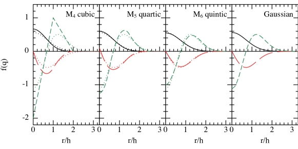
Figure 2: The $M_{4}$ (cubic, truncated at $2h$), $M_{5}$ (quartic, truncated at $2.5h$) and $M_{6}$ (quintic, truncated at $3h$) Schoenberg (1946) B-spline kernel functions (solid lines) and their first (long-dashed) and second (short-dashed) derivatives, compared to the Gaussian (right panel and dotted lines in other panels). Notice that although the “number of neighbours” increases in the $M_{5}$ and $M_{6}$ functions compared to the cubic spline, the smoothing scale $h$ retains the same meaning with respect to the Gaussian. Thus, using the higher order B-splines is a way to increase the smoothness of the kernel summations without altering the resolution length, and is very different to simply increasing the number of neighbours under the cubic spline.

2.3 Kernel functions with compact support

There are many kernel functions which fit this bill. The most well-used (for SPH at least) are the Schoenberg (1946) B-spline functions (Monaghan and Lattanzio, 1985; Monaghan, 1985, 2005), generated as the Fourier transform

$$M_{n}(x,h)=\frac{1}{2\pi}\int^{\infty}_{-\infty}\left[\frac{\sin{(kh/2)}}{kh/2}\right]^{n}\cos(kx){\rm d}k.$$ (5)

These give progressively better approximations to the Gaussian at higher $n$, both by increasing the radius of compact support and by increasing smoothness, since each function $M_{n}$ is continuous up to the $\{n-2\}$th derivatives. Since we minimally require continuity in at least the first and second derivatives, the lowest order B-spline useful for SPH is the $M_{4}$ (cubic) spline truncated at $2h$:

$$w(q)=\sigma\left\{\begin{array}[]{ll}\frac{1}{4}(2-q)^{3}-(1-q)^{3},&0\leq q<1;\\ \frac{1}{4}(2-q)^{3},&1\leq q<2;\\ 0.&q\geq 2,\end{array}\right.$$ (6)

where for convenience we use $W(|{\bf r}-{\bf r}^{\prime}|,h)\equiv\frac{1}{h^{d}}w(q)$, where $q=|{\bf r}-{\bf r}^{\prime}|/h$ and $\sigma$ is a normalisation constant given by $\sigma=[2/3,10/(7\pi),1/\pi]$ in $[1,2,3]$ dimensions. Next are the $M_{5}$ quartic, truncated at $2.5h$:

$$w(q)=\sigma\left\{\begin{array}[]{ll}\left(\frac{5}{2}-q\right)^{4}-5\left(\frac{3}{2}-q\right)^{4}+10\left(\frac{1}{2}-q\right)^{4},&0\leq q<\frac{1}{2};\\ \left(\frac{5}{2}-q\right)^{4}-5\left(\frac{3}{2}-q\right)^{4},&\frac{1}{2}\leq q<\frac{3}{2};\\ \left(\frac{5}{2}-q\right)^{4},&\frac{3}{2}\leq q<\frac{5}{2};\\ 0.&q\geq\frac{5}{2},\end{array}\right.$$ (7)

with normalisation $\sigma=[1/24,96/1199\pi,1/20\pi]$, and the $M_{6}$ quintic, truncated at $3h$:

$$w(q)=\sigma\left\{\begin{array}[]{ll}(3-q)^{5}-6(2-q)^{5}+15(1-q)^{5},&0\leq q<1;\\ (3-q)^{5}-6(2-q)^{5},&1\leq q<2;\\ (3-q)^{5},&2\leq q<3;\\ 0.&q\geq 3,\end{array}\right.$$ (8)

with normalisation $\sigma=[1/120,7/478\pi,1/120\pi]$ (e.g. Morris, 1996b). These kernel functions and their first and second derivatives are shown for comparison with the Gaussian in Fig. 2.

One important aspect to draw from our discussion so far is the clear meaning attached to the smoothing length $h$ as specifying the fall-off of the kernel weighting with respect to the particle separation. In particular, it is clear that referring to the “number of neighbours” does not have any meaning per se for Gaussian and Gaussian-like kernels: For the Gaussian the number of neighbours is in principle infinite, but there nevertheless exists a well-defined smoothing scale, $h$. The higher order B-splines (Fig. 2) also demonstrate that it is possible to change the “neighbour number” – by progressing to higher $n$ in the series – without changing the smoothing length. It is a widely-propagated myth that one can achieve formal convergence in SPH by “increasing the number of neighbours” (e.g. more slowly than the total number of particles). However, there are very important differences between simply “stretching” the cubic spline to accommodate a larger neighbour number – which amounts to changing the ratio of $h$ to particle spacing – and using a kernel that has a larger radius of compact support but retains the same $h$. That is, in no sense is the SPH density estimate (our “approach 3”) the same as approach 2 shown in Fig. 1b. We will return to this point later.

There are obviously other kernels, and other families of kernels, that satisfy the above properties (e.g. Dehnen, 2001). However, more detailed investigations into kernels (e.g. Fulk and Quinn, 1996) tend to merely confirm the points made above – namely that Bell-shaped, symmetric, monotonic kernels provide the best density estimates. We will examine the formal errors in the kernel density estimate shortly, but first we turn to the issue of setting the smoothing length, $h$.

2.4 Setting the smoothing length

Early SPH simulations (e.g. Gingold and Monaghan, 1977) simply employed a spatially constant resolution length $h$, though one which was allowed to change as a function of time according to the densest part of a calculation. However, as is evident from Fig. 1, it is clearly desirable to resolve both clustered and sparse regions evenly – that is, with a roughly constant ratio of $h$ to the mean local particle separation. Thus, a natural choice for setting the smoothing length is to relate to the local number density of particles, i.e.,

$$h({\bf r})\propto n({\bf r})^{-1/d};\hskip 28.45274ptn({\bf r})=\sum_{b}W\left[{\bf r}-{\bf r}_{b},h({\bf r})\right].$$ (9)

For equal mass particles, this is equivalent to making $h$ proportional to the density itself (since $1/n\equiv m/\rho$). Since in turn density is itself a function of smoothing length, this leads to the idea of an iterative summation to simultaneously obtain the (mutually dependent) $\rho({\bf r})$ and $h({\bf r})$ (Springel and Hernquist, 2002; Monaghan, 2002; Price and Monaghan, 2007). Computed at the location of particle $a$, we have a set of two simultaneous equations

$$\rho({\bf r}_{a})=\sum_{b}m_{b}W({\bf r}_{a}-{\bf r}_{b},h_{a});\hskip 28.45274pth({\bf r}_{a})=\eta\left(\frac{m_{a}}{\rho_{a}}\right)^{1/d},$$ (10)

where $\eta$ is a parameter specifying the smoothing length in units of the mean particle spacing $(m/\rho)^{1/d}$. These two equations can be solved simultaneously using standard root-finding methods such as Newton-Raphson or Bisection and most “modern” SPH codes employ such a procedure (for reasons that will become clear). Note that enforcing the relation given in (10) is approximately equivalent to keeping the “mass inside the smoothing sphere” constant (Springel and Hernquist, 2002), since for example in three dimensions

$$M_{tot}^{a}=\int_{V_{a}}\rho dV\approx\frac{4}{3}\pi R_{kern}^{3}\rho_{a},$$ (11)

where $R_{kern}$ is the kernel radius ($2h$ for the cubic spline), so $M_{tot}=const$ implies $h^{3}\rho=const$. Since for equal mass particles $M_{tot}=mN_{neigh}$, this also means that the number of neighbours should be approximately constant if the relationship in (10) (or for unequal mass particles, Eq. 9) is enforced. Indeed a “number of neighbours” parameter can be used in place of the parameter $\eta$, using

$$N_{neigh,1D}=2\zeta\eta;\hskip 28.45274ptN_{neigh,2D}=\pi(\zeta\eta)^{2};\hskip 28.45274ptN_{neigh,3D}=\frac{4}{3}\pi(\zeta\eta)^{3},$$ (12)

where $\zeta$ is the compact support radius in units of $h$ (i.e., $\zeta=2$ for the cubic spline). However, this is problematic for several reasons. Firstly it gives the dangerous impression that $N_{neigh}$ is a free parameter unrelated to $h$, whereas changing $N_{neigh}$ explicitly changes $h$ – more specifically, the ratio of $h$ to particle spacing (i.e., $\eta$) – and corresponds to “stretching” the cubic spline as discussed above. Secondly, whereas $\eta$ carries the same meaning in $1$, $2$ and $3$ dimensions, the $N_{neigh}$ parameter changes, making it difficult to relate the results of one and two dimensional test problems to three dimensional simulations. Thirdly, $N_{neigh}$ is often used as an integer parameter, whereas it is clear from (10) that the $h-\rho$ (or $h-n$) iterations can be performed to arbitrary accuracy (that is, to fractional neighbour numbers) – which is also necessary if one is to assume that the relationship is differentiable. Finally, $N_{neigh}$ is only related to the true number of neighbours so long as the (number) density of particles within the smoothing sphere is approximately constant (that is, so far as the integral in Eq. 11 can be approximated by $\frac{4}{3}\pi R^{3}\rho$). So at best a $N_{neigh}$ parameter only characterises the mean neighbour number – and there can be strong fluctuations about this mean, for example in strong density gradients.

Earlier adaptive SPH implementations employed density estimates involving either an average smoothing length $\bar{h}=\frac{1}{2}\left(h_{a}+h_{b}\right)$ (e.g. Benz, 1990) or an average of the smoothing kernels $\overline{W}_{ab}=\frac{1}{2}\left[W_{ab}(h_{a})+W_{ab}(h_{b})\right]$ (e.g. Hernquist and Katz, 1989). However, this inevitably leads to heuristic methods for setting the smoothing length itself – for example by evolving the time derivative of Eq. 10 with “corrections” to try to keep the neighbour number approximately constant (e.g. Benz, 1990) or simply enforcing a constant neighbour number either approximately or exactly (e.g. Hernquist and Katz, 1989). It also considerably complicated attempts to incorporate derivatives of the smoothing length – necessary for exact energy and entropy conservation – into the equations of motion (Nelson and Papaloizou, 1994). By contrast, the mathematical meaning of Eqs. (10) is clear and it is straightforward to take derivatives involving the smoothing length.

Finally, the density estimate computed via (10) is time-independent, depending only on particle positions and masses and thus explicitly answering our original question of how to compute a density field from point mass particles. This also means it has wide applicability to many other problems beyond SPH – for example Price and Federrath (2010) use it to construct a density field from Lagrangian tracer particles in grid-based simulations of supersonic turbulence; and it forms the basis of the adaptive gravitational force softening method introduced by Price and Monaghan (2007).

2.5 Errors in the density estimate

The formal errors in the density estimate may be determined by writing the density summation as an integral – that is, assuming $m\equiv\rho dV$ and that the summation is well sampled, giving

$$\langle\rho({\bf r})\rangle=\int\rho({\bf r}^{\prime})W({\bf r}-{\bf r}^{\prime},h)dV^{\prime}.$$ (13)

where $\langle..\rangle$ refers to a smoothed estimate. Expanding $\rho({\bf r}^{\prime})$ in a Taylor series about ${\bf r}$, we have

$$\langle\rho({\bf r})\rangle=\rho({\bf r})\int W({\bf r}-{\bf r}^{\prime},h)dV^{\prime}+\nabla\rho({\bf r})\cdot\int({\bf r}^{\prime}-{\bf r})W({\bf r}-{\bf r}^{\prime},h)dV^{\prime}+\nabla^{\alpha}\nabla^{\beta}\rho({\bf r})\int\delta{\bf r}^{\alpha}\delta{\bf r}^{\beta}W({\bf r}-{\bf r}^{\prime},h)dV^{\prime}+\mathcal{O}(h^{3})$$ (14)

so that if the normalisation condition (3) is satisfied and a symmetric kernel $W({\bf r}-{\bf r}^{\prime},h)=W({\bf r}^{\prime}-{\bf r},h)$ is used such that the odd error terms vanish, the error in the density interpolant is $\mathcal{O}(h^{2})$. In principle it is also possible to construct kernels such that the second moment is also zero, resulting in errors of $\mathcal{O}(h^{4})$ (see Monaghan, 1985). The disadvantage of such kernels is that the kernel function becomes negative in some part of the domain, resulting in a potentially negative density evaluation. Achieving such higher order in practice also requires that the kernel is extremely well sampled, leading to substantial additional cost requirements. One possibility given the iterations necessary to solve (10) would be to automatically switch between high order and low order kernels during the iterations (e.g. if a negative density occurs), thus leading to high order interpolation in smooth regions but a low order interpolation where the density changes rapidly. The errors in the discrete version are discussed further in Sec. 4.3.

2.6 Alternatives to the SPH density estimate

Finally, it should be noted that the three general approaches described in Sec. 2.2 are not the only methods that can be employed for estimating the density. A fourth alternative that has received recent attention involves the use of Delaunay or Voronoi tessellation – the former proposed by Pelupessy et al. (2003) and the latter developed into a full hydrodynamics scheme by Serrano et al. (2005) and Heß and Springel (2010). These are promising approaches that in principle can offer all the same advantages as SPH in terms of exact conservation – since it can be derived similarly from a Hamiltonian formulation – but with an improved density estimate and an exact partition of unity.

3 From density to equations of motion

The reader at this point may wonder why we have spent so long discussing nothing else except the density estimate. The reason is that this is the only real freedom one has if one wishes to obtain a fully conservative SPH algorithm, at least in the absence of dissipative terms. This is because the rest of the SPH algorithm can be derived entirely from the density estimate.

3.1 The discrete Lagrangian

The derivation starts with the discrete Lagrangian. As is usual, the Lagrangian is simply given by

$$L=T-V,$$ (15)

where $T$ and $V$ are the kinetic and potential (in this case, thermal) energies respectively. For a system of point masses with velocity ${\bf v}\equiv d{\bf r}/dt$ and internal energy per unit mass $u$, we have

$$L=\sum_{b}m_{b}\left[\frac{1}{2}v_{b}^{2}-u_{b}(\rho_{b},s_{b})\right],$$ (16)

where in general the thermal energy $u$ can be specified as a function of the thermodynamic variables $\rho$ and $s$ (the density and entropy, respectively). Although (16) can be considered as a discrete version of the continuum Lagrangian for hydrodynamics (e.g. Eckart, 1960; Salmon, 1988; Morrison, 1998)

$$L=\int\left[\rho v^{2}-\rho u(\rho,s)\right]{\rm dV},$$ (17)

one is free to consider the discrete Hamiltonian system, it’s associated symmetries and equations of motion directly – that is, without explicit reference to the continuum system. In other words the Hamiltonian properties are directly present in the discrete system and the motions will be constrained to obey the symmetries and conservation properties of the discrete Lagrangian.

3.2 Least action principle and the Euler-Lagrange equations

The equations of motion for such a system can be derived from the principle of least action, that is minimising the action

$$S=\int L{\rm dt},$$ (18)

such that $\delta S=\int\delta L{\rm dt}=0$, where $\delta$ is a variation with respect to a small change in the particle coordinates $\delta{\bf r}$. Assuming that the Lagrangian can be written as a differentiable function of the particle positions ${\bf r}$ and velocities ${\bf v}$, we have

$$\delta S=\int\left(\frac{\partial L}{\partial{\bf v}}\cdot\delta{\bf v}+\frac{\partial L}{\partial{\bf r}}\cdot\delta{\bf r}\right){\rm dt}=0.$$ (19)

Integrating by parts, using the fact that $\delta{\bf v}=d(\delta{\bf r})/dt$, where $d/dt\equiv\partial/\partial t+{\bf v}\cdot\nabla$ gives

$$\delta S=\int\left\{\left[-\frac{d}{dt}\left(\frac{\partial L}{\partial{\bf v}}\right)+\frac{\partial L}{\partial{\bf r}}\right]\cdot\delta{\bf r}\right\}{\rm dt}+\left[\frac{\partial L}{\partial{\bf v}}\cdot\delta{\bf r}\right]^{t}_{t_{0}}=0.$$ (20)

So if we assume that the variation vanishes at the start and end times, then since the variation $\delta{\bf r}$ is arbitrary, the equations of motion are given by the Euler-Lagrange equations, here taken with respect to particle $a$:

$$\frac{d}{dt}\left(\frac{\partial L}{\partial{\bf v}_{a}}\right)-\frac{\partial L}{\partial{\bf r}_{a}}=0.$$ (21)

We have somewhat laboured the point here because it is important to understand the assumptions we have made by employing the Euler-Lagrange equations to derive the equations of motion. The first is that in using Eq. 21 we are not explicitly considering the discreteness of the time integral. So when we refer below to “exact conservation” (e.g. of energy and momentum) we mean “solely governed by errors in the time integration scheme”.

The other, more critical, assumption we have made in employing (21) is that the Lagrangian is differentiable. This means that we have explicitly excluded the possibility of discontinuous solutions to the equations of motion. What this means in practice is that any discontinuities present in the system (for example in the initial conditions) require careful treatment – for example by adding dissipative terms that smooth discontinuities to a resolvable scale (i.e., a few $h$) such that they can be treated as no longer discontinuous. We give some practical examples of this in Sec. 6.3. A better way would be to account for the neglected surface integral terms directly in the Lagrangian (e.g. Kats, 2001), though it is not clear how one would go about doing so in an SPH context.

3.3 Equations of motion

All that remains in order to derive the equations of motion is to compute the derivatives in (21) by writing the terms in the Lagrangian as a function of the particle coordinates and velocities. From (16) we have

$$\frac{\partial L}{\partial{\bf v}_{a}}=m_{a}{\bf v}_{a};\hskip 28.45274pt\frac{\partial L}{\partial{\bf r}_{a}}=-\sum_{b}m_{b}\left.\frac{\partial u_{b}}{\partial\rho_{b}}\right|_{s}\frac{\partial\rho_{b}}{\partial{\bf r}_{a}},$$ (22)

the latter since $u$ is a function of $\rho$ and $s$, and we assume that the entropy $s$ is constant (i.e., no dissipation). Note that the former gives the canonical momenta of the system (${\bf p}\equiv\partial L/\partial{\bf v}$). This step is straightforward for hydrodynamics, but it can also be used to derive the conservative momentum variable in the case of more complicated physics – for example in relativistic SPH (e.g. Monaghan and Price, 2001; Rosswog, 2009).

3.3.1 Thermodynamics of the fluid

From the first law of thermodynamics we have

$$dU=TdS-PdV,$$ (23)

where $\delta Q\equiv TdS$ is the heat added to the system (per unit volume) and $\delta W\equiv PdV$ is the work done by expansion and compression of the fluid. We do not compute the volume directly in SPH, but instead we can use the volume estimate given by $V=m/\rho$ and thus the change in volume given by $dV=-m/\rho^{2}d\rho$. Using quantities per unit mass instead of per unit volume (i.e., $du$ instead of $dU$), we have

$$du=Tds+\frac{P}{\rho^{2}}d\rho,$$ (24)

such that at constant entropy, the change in thermal energy is given by

$$\left.\frac{\partial u_{b}}{\partial\rho_{b}}\right|_{s}=\frac{P}{\rho^{2}}.$$ (25)

3.3.2 The density gradient

So far we have not made any explicit reference to SPH or kernel interpolation. This arises because of the spatial derivative of the density (Eq. 22), that we obtain by differentiating our density estimate (Eq. 10). Noting that we are taking the gradient of the density estimate at particle $b$ with respect to the coordinates of particle $a$, this is given by

$$\frac{\partial\rho_{b}}{\partial{\bf r}_{a}}=\frac{1}{\Omega_{b}}\sum_{c}m_{c}\frac{\partial W_{bc}(h_{b})}{\partial{\bf r}_{a}}\left(\delta_{ba}-\delta_{ca}\right),$$ (26)

where $W_{bc}(h_{b})\equiv W({\bf r}_{b}-{\bf r}_{c},h_{b})$, $\delta_{ba}$ is a Dirac delta function referring to the particle indices and we have assumed that the smoothing length is itself a function of density [i.e., $h=h(\rho)$], giving a term accounting for the gradient of the smoothing length given by

$$\Omega_{a}\equiv\left[1-\frac{\partial h_{a}}{\partial\rho_{a}}\sum_{b}m_{b}\frac{\partial W_{ab}(h_{a})}{\partial h_{a}}\right],$$ (27)

where for the standard $h-\rho$ relationship (Eq. 10) the derivative is given by

$$\frac{\partial h}{\partial\rho}=-\frac{h}{\rho d},$$ (28)

where $d$ is the number of spatial dimensions.

3.3.3 Equations of motion

Using (26) and (25) in (22) we have

$$\frac{\partial L}{\partial{\bf r}_{a}}=-\sum_{b}m_{b}\frac{P_{b}}{\Omega_{b}\rho_{b}^{2}}\sum_{c}m_{c}\frac{\partial W_{bc}(h_{b})}{\partial{\bf r}_{a}}\left(\delta_{ba}-\delta_{ca}\right),$$ (29)

which, upon simplification, gives the equations of motion from the Euler-Lagrange equations in the form

$$\frac{d{\bf v}_{a}}{dt}=-\sum_{b}m_{b}\left[\frac{P_{a}}{\Omega_{a}\rho_{a}^{2}}\frac{\partial W_{ab}(h_{a})}{\partial{\bf r}_{a}}+\frac{P_{b}}{\Omega_{b}\rho_{b}^{2}}\frac{\partial W_{ab}(h_{b})}{\partial{\bf r}_{a}}\right].$$ (30)

For a constant smoothing length these equations simplify to the standard SPH expression (Monaghan, 1992)

$$\frac{d{\bf v}_{a}}{dt}=-\sum_{b}m_{b}\left(\frac{P_{a}}{\rho_{a}^{2}}+\frac{P_{b}}{\rho_{b}^{2}}\right)\nabla_{a}W_{ab}.$$ (31)

3.3.4 Conservation properties

Although we cannot yet provide interpretation to the equations of motion so derived, we can note a number of interesting properties. The first is that the total linear momentum is conserved exactly, since

$$\frac{d}{dt}\sum_{a}m_{a}{\bf v}_{a}=\sum_{a}m_{a}\frac{d{\bf v}_{a}}{dt}=-\sum_{a}\sum_{b}m_{a}m_{b}\left(\frac{P_{a}}{\rho_{a}^{2}}+\frac{P_{b}}{\rho_{b}^{2}}\right)\nabla_{a}W_{ab}=0,$$ (32)

where the double summation is zero because of the antisymmetry in the kernel gradient (the reader may verify that this is also true for Eq. 30). Secondly, the total angular momentum is also exactly conserved, since

$$\frac{d}{dt}\sum_{a}{\bf r}_{a}\times m_{a}{\bf v}_{a}=\sum_{a}m_{a}\left({\bf r}_{a}\times\frac{d{\bf v}_{a}}{dt}\right)=-\sum_{a}\sum_{b}m_{a}m_{b}\left(\frac{P_{a}}{\rho_{a}^{2}}+\frac{P_{b}}{\rho_{b}^{2}}\right){\bf r}_{a}\times({\bf r}_{a}-{\bf r}_{b})\tilde{F}_{ab}=0,$$ (33)

where for convenience we have written the gradient of the kernel in the form $\nabla_{a}W_{ab}={\bf r}_{ab}\tilde{F}_{ab}$, and the last term is zero again because of the antisymmetry in the double summation [since (${\bf r}_{a}\times{\bf r}_{b})=-({\bf r}_{b}\times{\bf r}_{a}$)].

The above conservation properties follow directly from the symmetries in the original Lagrangian and (by extension) the SPH density estimate (Eq. 10) – linear momentum conservation because the Lagrangian and density estimate are invariant to translations, and angular momentum conservation because they are invariant to rotations of the particle coordinates. This is important in thinking about possible modifications to the SPH scheme (for example using non-spherical kernels would result in the non-conservation of angular momentum because the density estimate would no longer be invariant to rotations).

Finally, we note that although the equations of motion depend only on the relative positions of the particles, they do depend on the absolute value of the pressure. That is, Eqs. (30) and (31) contain a force between the particles that is non-zero even when the pressure is constant. We discuss the importance of – and problems associated with – this ‘spurious’ force in Sec. 5.

3.4 Energy equation

The remaining part of the (dissipationless) SPH algorithm – the energy equation – can also be derived from the Hamiltonian dynamics. Here we have the choice of evolving either the thermal energy $u$, the total specific energy $e=\frac{1}{2}v^{2}+u$ or an entropy variable $K=P/\rho^{\gamma}$. Equations for each of these can be derived, as given below. It is important to note, however, that – provided the equations are derived from the Lagrangian formulation – there is no difference in SPH between evolving any of these variables, except due to the timestepping algorithm. This is rather different to the situation in an Eulerian code where the finite differencing of the advection terms mean that writing the equations in conservative form (i.e., using $e$) differs more substantially from evolving $u$ or $K$.

3.4.1 Internal energy

The evolution equation for the internal energy (in the absence of dissipation), from Eq. 25, is given by

$$\frac{du_{a}}{dt}=\frac{P_{a}}{\rho_{a}^{2}}\frac{d\rho_{a}}{dt}.$$ (34)

Taking the time derivative of the density sum (Eq. 10), we obtain an evolution equation for $u$ of the form

$$\frac{du_{a}}{dt}=\frac{P_{a}}{\Omega_{a}\rho_{a}^{2}}\sum_{b}m_{b}({\bf v}_{a}-{\bf v}_{b})\cdot\nabla_{a}W_{ab}(h_{a}).$$ (35)

3.4.2 Total energy

The conserved (total) energy is found from the Lagrangian via the Hamiltonian

$$H=\sum_{a}{\bf v}_{a}\cdot\frac{\partial L}{\partial{\bf v}_{a}}-L=\sum_{a}m_{a}\left(\frac{1}{2}v_{a}^{2}+u_{a}\right),$$ (36)

which is simply the total energy of the SPH particles, $E$, since the Lagrangian does not explicitly depend on the time. Taking the (Lagrangian) time derivative of (36), we have

$$\frac{dE}{dt}=\sum_{a}m_{a}\left({\bf v}_{a}\cdot\frac{d{\bf v}_{a}}{dt}+\frac{du_{a}}{dt}\right).$$ (37)

Substituting (30) and (35) and rearranging we find

$$\frac{dE}{dt}=\sum_{a}m_{a}\frac{de_{a}}{dt}=-\sum_{a}\sum_{b}m_{a}m_{b}\left[\frac{P_{a}}{\Omega_{a}\rho_{a}^{2}}{\bf v}_{b}\cdot\nabla_{a}W_{ab}(h_{a})+\frac{P_{b}}{\Omega_{b}\rho_{b}^{2}}{\bf v}_{a}\cdot\nabla_{a}W_{ab}(h_{b})\right]=0.$$ (38)

This equation shows that the total energy is also exactly conserved by the SPH scheme (where the double sum is zero again because of the antisymmetry with respect to the particle index, similar to the conservation of linear momentum discussed above). The conservation of total energy is a consequence of the symmetry of the Lagrangian (16) with respect to time as well as invariance under time translations. Eq. 38 also shows that the dissipationless evolution equation for the specific energy $e$ is given by

$$\frac{de_{a}}{dt}=-\sum_{b}m_{b}\left[\frac{P_{a}}{\Omega_{a}\rho_{a}^{2}}{\bf v}_{b}\cdot\nabla_{a}W_{ab}(h_{a})+\frac{P_{b}}{\Omega_{b}\rho_{b}^{2}}{\bf v}_{a}\cdot\nabla_{a}W_{ab}(h_{b})\right].$$ (39)

3.4.3 Entropy

For the specific case of an ideal gas equation of state, where

$$P=K(s)\rho^{\gamma},$$ (40)

it is possible to use the function $K(s)$ as the evolved variable (Springel and Hernquist, 2002), where the evolution of $K$ is given by

$$\frac{dK}{dt}=\frac{\gamma-1}{\rho^{\gamma-1}}\left(\frac{du}{dt}-\frac{P}{\rho^{2}}\frac{d\rho}{dt}\right)=\frac{\gamma-1}{\rho^{\gamma-1}}\left(\frac{du}{dt}\right)_{diss}.$$ (41)

The thermal energy is then evaluated using

$$u=\frac{K}{\gamma-1}\rho^{\gamma-1}.$$ (42)

Since $dK/dt=0$ in the absence of dissipation, using $K$ has the advantage that the evolution is independent of the time-integration algorithm. The disadvantage is that it is more difficult to apply to non-ideal equations of state. This is sometimes referred to as the ‘entropy-conserving’ form of SPH (after Springel and Hernquist, 2002) – which is somewhat misleading since the entropy per particle is also exactly conserved if (35) or (39) are used provided the smoothing length gradient terms are correctly accounted for (i.e., $du/dt-P/\rho^{2}d\rho/dt=0$), apart from minor differences arising from the timestepping scheme. So the term ‘entropy-conserving’ more correctly refers to the correct accounting of smoothing length gradient terms and a consistent formulation of the energy equation than whether or not an entropy variable is evolved.

3.5 Summary

In summary, our full system of equations for $\rho$, ${\bf v}$ and $u$ is given by

$$\rho_{a} = \sum_{b}m_{b}W({\bf r}_{a}-{\bf r}_{b},h_{a});\hskip 28.45274pth=h(\rho),$$ (43)

$$\frac{d{\bf v}_{a}}{dt} = -\sum_{b}m_{b}\left[\frac{P_{a}}{\Omega_{a}\rho_{a}^{2}}\nabla_{a}W_{ab}(h_{a})+\frac{P_{b}}{\Omega_{b}\rho_{b}^{2}}\nabla_{a}W_{ab}(h_{b})\right],$$ (44)

$$\frac{du_{a}}{dt} = \frac{P_{a}}{\Omega_{a}\rho_{a}^{2}}\sum_{b}m_{b}({\bf v}_{a}-{\bf v}_{b})\cdot\nabla_{a}W_{ab}(h_{a}),$$ (45)

where in place of (45) we could equivalently use either (39) or (41). The reader will note that so far we have not even mentioned the continuum equations of hydrodynamics – we have merely specified the physics that goes into the Lagrangian (Eq. 16), the thermodynamics of the fluid (Eq. 24) and the manner in which the density is calculated (Eq. 10) and with these have directly derived the discrete equations of the Hamiltonian system. In order to interpret them we need to know how to translate our SPH equations (43)–(45) into their continuum equivalents.

Before doing so, it is worth recapping briefly the assumptions we have made in arriving at (43)–(45) from the Lagrangian (Eq. 16). These are

1. That the time integration and thus time derivatives, $d/dt$, are computed exactly (though this assumption can in principle be relaxed);

2. That the Lagrangian, and by implication the density and thermal energies are differentiable;

3. That there is no change in entropy, such that the first law of thermodynamics $du=PdV$ is satisfied, and that the change in particle volume is given by $dV=-m/\rho^{2}d\rho$.

The second and third assumptions in particular come into play in dealing with shocks and other kinds of discontinuities, which will we discuss further in Sec 6.3.

3.6 Alternative formulations

Within the constraints of a Hamiltonian SPH formulation, it is clear that there is only a very limited freedom to change the algorithm without breaking some of the conservation properties of the scheme. So there are only two basic ways to change the (dissipationless) algorithm that are consistent with the Hamiltonian approach (other than changing the first law of thermodynamics): i) change the way the density is calculated or ii) introduce additional physical terms, and associated constraints, into the Lagrangian. Examples of the former are the consistent formulation of variable smoothing length terms – requiring the iterative solution of $h$ and $\rho$ in the density sum (Eq. 10) – by Springel and Hernquist (2002) and Monaghan (2002), and an incorporation of boundary correction forces (Kulasegaram et al., 2004). Examples of the latter include consistent derivations of relativistic SPH (Monaghan and Price, 2001; Rosswog, 2009), adaptive gravitational force softening (Price and Monaghan, 2007), sub-resolution turbulence models (Monaghan, 2002, 2004) and MHD (Price and Monaghan, 2004b; Price, 2010).

4 Kernel interpolation theory and SPH derivatives

The usual way of introducing SPH is to start with a formal discussion of kernel interpolation theory. We have taken a rather different approach in this review and will introduce this theory primarily only to interpret the equations that we have derived from the discrete Lagrangian, and also as a way of discussing how to go about introducing additional physics. However, we will not use the linear error properties of the interpolation scheme to define the method – apart from our construction of the density estimate discussed above. The reason is that focussing on linear errors over the Hamiltonian properties of SPH misses some of the subtle but important non-linear behaviour that makes SPH work in practice, which we will come to discuss. However, first let us proceed:

4.1 Kernel interpolation: the basics

Kernel interpolation theory starts with the identity

$$A({\bf r})=\int A({\bf r^{\prime}})\delta({\bf r}-{\bf r}^{\prime})d{\bf r}^{\prime},$$ (46)

where $A$ is an arbitrary scalar variable and $\delta$ refers to the Dirac delta function. This integral is then approximated by replacing the delta function with a smoothing kernel $W$ with finite width $h$, i.e.,

$$A({\bf r})=\int A({\bf r}^{\prime})W({\bf r}-{\bf r}^{\prime},h)d{\bf r^{\prime}}+O(h^{2}).$$ (47)

where $W$ has the property

$$\lim_{h\to 0}W({\bf r}-{\bf r}^{\prime},h)=\delta({\bf r}-{\bf r}^{\prime}),$$ (48)

and normalisation $\int_{V}WdV^{\prime}=1$, as we have already discussed in Sec. 2.2. Finally the integral interpolant (Eq. 47) is discretised onto a finite set of interpolation points (the particles) by replacing the integral by a summation and the mass element $\rho dV$ with the particle mass $m$, i.e.

$$\langle A({\bf r})\rangle = \int\frac{A({\bf r^{\prime}})}{\rho({\bf r^{\prime}})}W({\bf r}-{\bf r}^{\prime},h)\rho({\bf r^{\prime}})d{\bf r^{\prime}},$$ (49)

$$\approx \sum^{N_{neigh}}_{b=1}m_{b}\frac{A_{b}}{\rho_{b}}W({\bf r}-{\bf r}_{b},h),$$

This ‘summation interpolant’ is the basis of all SPH formalisms. The reader will note that choosing $A=\rho$ results in the SPH density estimate (Eq. 10). In this paper we have argued that the density estimate (10) is in some sense more fundamental than the summation interpolant (49), since the equations of motion can be derived without reference to (49). On the other hand, the summation interpolant gives a general way of a interpolating a quantity at any point in space $A({\bf r})$ from quantities defined solely on the particles themselves (i.e., $A_{b}$, $\rho_{b}$, $m_{b}$), and in turn to a general way of formulating SPH equations. In particular, gradient terms may be straightforwardly calculated by taking the derivative of (49), giving

$$\nabla A({\bf r}) = \frac{\partial}{\partial{\bf r}}\int\frac{A({\bf r^{\prime}})}{\rho({\bf r^{\prime}})}W({\bf r}-{\bf r}^{\prime},h)\rho({\bf r^{\prime}})d{\bf r^{\prime}}+O(h^{2}),$$ (50)

$$\approx \sum_{b}m_{b}\frac{A_{b}}{\rho_{b}}\nabla W({\bf r}-{\bf r}_{b},h).$$ (51)

For vector quantities the expressions are similar, simply replacing $A$ with ${\bf A}$ in (49), giving

$${\bf A}({\bf r}) \approx \sum_{b}m_{b}\frac{{\bf A}_{b}}{\rho_{b}}W({\bf r}-{\bf r}_{b},h),$$ (52)

$$\nabla\cdot{\bf A}({\bf r}) \approx \sum_{b}m_{b}\frac{{\bf A}_{b}}{\rho_{b}}\cdot\nabla W({\bf r}-{\bf r}_{b},h),$$ (53)

$$\nabla\times{\bf A}({\bf r}) \approx -\sum_{b}m_{b}\frac{{\bf A}_{b}}{\rho_{b}}\times\nabla W({\bf r}-{\bf r}_{b},h),$$ (54)

$$\nabla^{j}A^{i}({\bf r}) \approx \sum_{b}m_{b}\frac{A^{i}_{b}}{\rho_{b}}\nabla^{j}W({\bf r}-{\bf r}_{b},h).$$ (55)

The problem is that using these expressions ‘as is’ in general leads to quite poor gradient estimates, and we can do better by considering the errors in the above approximations. However, the basic interpolants given above give us a general way of interpreting SPH expressions such as those derived in Sec. 3.

4.2 Interpretation of the Hamiltonian SPH equations

We are now able to provide interpretation to our Hamiltonian-SPH equations (43)–(45) derived in Sec. 3 using the basic identities (51)–(54). We begin with the density summation (43). Taking the time derivative, we have

$$\frac{d\rho_{a}}{dt}=\frac{1}{\Omega_{a}}\sum_{b}m_{b}\left({\bf v}_{a}-{\bf v}_{b}\right)\cdot\nabla_{a}W_{ab}(h_{a}),$$ (56)

which for a constant smoothing length simplifies to

$$\frac{d\rho_{a}}{dt}=\sum_{b}m_{b}\left({\bf v}_{a}-{\bf v}_{b}\right)\cdot\nabla_{a}W_{ab}(h).$$ (57)

Using (53) we can translate each of the terms according to

$$\frac{d\rho_{a}}{dt}={\bf v}_{a}\cdot\sum_{b}\frac{m_{b}}{\rho_{b}}\rho_{b}\nabla_{a}W_{ab}-\sum_{b}\frac{m_{b}}{\rho_{b}}(\rho_{b}{\bf v}_{b})\cdot\nabla_{a}W_{ab}\approx{\bf v}_{a}\cdot\nabla\rho-\nabla\cdot(\rho{\bf v})\approx-\rho_{a}(\nabla\cdot{\bf v})_{a}.$$ (58)

So remarkably (57) (and by inference, 56) – which we obtained simply by taking the time derivative of the density sum – represents a (particular) SPH discretisation of the continuity equation. Indeed, the density summation is therefore an exact, time-independent, solution to the SPH continuity equation. This should not be particularly surprising, since the continuity equation derives from the conservation of mass, which is self-evidently enforced on the particles since $m$ is fixed.

Our force term (44), assuming a constant $h$ (Eq. 31) can be translated according to

$$-\sum_{b}m_{b}\left(\frac{P_{a}}{\rho_{a}^{2}}+\frac{P_{b}}{\rho_{b}^{2}}\right)\nabla_{a}W_{ab}\approx-\frac{P}{\rho^{2}}\nabla\rho-\nabla\left(\frac{P}{\rho}\right)\approx-\frac{\nabla P}{\rho},$$ (59)

where we have used the basic identity (51) to translate the two terms into their continuum equivalents.

Finally, the thermal energy equation (45) can be translated, from (34) and (58), giving

$$\frac{du}{dt}=-\frac{P}{\rho}\nabla\cdot{\bf v}.$$ (60)

In other words, it is evident that the Lagrangian has indeed given us valid discretisations for the equations of hydrodynamics, and therefore that the equations of our Hamiltonian system (43)–(45) do indeed solve these equations in discrete form – a remarkable achievement given the relatively few assumptions that were made. Yet the discretisations we derived are clearly not the basic ones arising from kernel interpolation theory (51)–(54). In order to examine the errors in these discretisations we need to understand the errors arising from the basic gradient operators, and how more general derivative operators can be constructed.

4.3 Errors

The errors introduced by the approximation (47) are similar to those in the density estimate (Sec. 2.5). That is, if we expand $A({\bf r}^{\prime})$ in a Taylor series about ${\bf r}$ (Benz, 1990; Monaghan, 1992), we find

$$\langle A({\bf r})\rangle=\int\left[A({\bf r})+({\bf r}^{\prime}-{\bf r})^{\alpha}\frac{\partial A}{\partial{\bf r}^{\alpha}}+\frac{1}{2}({\bf r}^{\prime}-{\bf r})^{\alpha}({\bf r}^{\prime}-{\bf r})^{\beta}\frac{\partial^{2}A}{\partial{\bf r}^{\alpha}\partial{\bf r}^{\beta}}+\mathcal{O}(({\bf r}-{\bf r}^{\prime})^{3})\right]W({\bf r}-{\bf r}^{\prime},h)\mathrm{d{\bf r}^{\prime}},$$ (61)

such that for symmetric $W\equiv W(|{\bf r}-{\bf r}^{\prime}|,h)$ and normalised ($\int WdV^{\prime}=1$) kernels we have

$$\langle A({\bf r})\rangle=A({\bf r})+\frac{1}{2}\frac{\partial^{2}A}{\partial{\bf r}^{\alpha}\partial{\bf r}^{\beta}}\int({\bf r}^{\prime}-{\bf r})^{\alpha}({\bf r}^{\prime}-{\bf r})^{\beta}W(|{\bf r}-{\bf r}^{\prime}|,h)\mathrm{d{\bf r}^{\prime}}+\mathcal{O}[({\bf r}^{\prime}-{\bf r})^{4}],$$ (62)

giving an interpolation that is second order accurate [$\mathcal{O}(h^{2})$] unless higher order kernels are used (see Sec. 2.5). However, the errors in the discrete version (Eq. 49) are not identical, since they depend on the degree to which the discrete summations approximate the integrals – specifically on the degree to which the discrete normalisation conditions are satisfied. Following Price (2004) we can perform a similar analysis on the summation interpolant (49, here assumed to be computed on particle $a$) by expanding $A_{b}$ in a Taylor series around ${\bf r}_{a}$, giving

$$\langle A_{a}\rangle=\sum_{b}m_{b}\frac{A_{b}}{\rho_{b}}W_{ab}=A_{a}\sum_{b}\frac{m_{b}}{\rho_{b}}W_{ab}+\nabla A_{a}\cdot\sum_{b}\frac{m_{b}}{\rho_{b}}({\bf r}_{b}-{\bf r}_{a})W_{ab}+\mathcal{O}(h^{2}).$$ (63)

This shows that in practice, the interpolation will only truly be second order accurate if the conditions

$$\sum_{b}\frac{m_{b}}{\rho_{b}}W_{ab}\approx 1;\hskip 28.45274pt\textrm{and}\hskip 28.45274pt\sum_{b}\frac{m_{b}}{\rho_{b}}({\bf r}_{b}-{\bf r}_{a})W_{ab}\approx 0,$$ (64)

hold. The degree to which this is true depends strongly on the particle distribution within the kernel radius, and the properties of the kernel when a finite number of neighbours are employed – in particular, the ratio of smoothing length to particle spacing $\Delta p$. Fig. 3 shows the first condition computed for the B-spline kernels and the Gaussian as a function of $h/\Delta p$ in 1D (solid/black lines), showing that in general the above conditions are maintained very well, provided the particles are regular. Thus, maintaining a regular particle arrangement, together with an appropriate choice of $h/\Delta p$, can be very important in obtaining accurate results with SPH. Used another way, the conditions (64) are essentially the criteria for a ‘good density kernel’ – that is, a good density kernel is one which satisfies these conditions well given the typical particle distributions encountered in SPH. Note that the second of these is much easier to satisfy than the first, since it requires only a reasonably symmetric particle distribution to be satisfied. In general reasonable fulfilment of the first condition amounts to the conditions 1)–3) on the density kernel described in Sec. 2.2.

The errors resulting from the gradient interpolation (50) may be estimated in a similar manner by again expanding $A({\bf r}^{\prime})$ in a Taylor series about ${\bf r}$, giving

$$\nabla A({\bf r}) = \int\left[A({\bf r})+({\bf r}^{\prime}-{\bf r})^{\alpha}\frac{\partial A}{\partial{\bf r}^{\alpha}}+\frac{1}{2}({\bf r}^{\prime}-{\bf r})^{\beta}({\bf r}^{\prime}-{\bf r})^{\gamma}\frac{\partial^{2}A}{\partial{\bf r}^{\beta}\partial{\bf r}^{\gamma}}+\mathcal{O}[({\bf r}-{\bf r}^{\prime})^{3}]\right]\nabla W(|\mathbf{r-r^{\prime}}|,h)d{\bf r}^{\prime},$$ (65)

$$= A({\bf r})\int\nabla Wd{\bf r}^{\prime}+\frac{\partial A}{\partial{\bf r}^{\alpha}}\int({\bf r}^{\prime}-{\bf r})^{\alpha}\nabla W\mathrm{d{\bf r}^{\prime}}+\frac{1}{2}\frac{\partial^{2}A}{\partial{\bf r}^{\beta}\partial{\bf r}^{\gamma}}\int({\bf r}^{\prime}-{\bf r})^{\beta}({\bf r}^{\prime}-{\bf r})^{\gamma}\nabla W\mathrm{d{\bf r}^{\prime}}+\mathcal{O}[({\bf r}^{\prime}-{\bf r})^{3}],$$

$$= \nabla A({\bf r})+\frac{1}{2}\frac{\partial^{2}A}{\partial{\bf r}^{\beta}\partial{\bf r}^{\gamma}}\int({\bf r}^{\prime}-{\bf r})^{\beta}({\bf r}^{\prime}-{\bf r})^{\gamma}\nabla W(r)\mathrm{d{\bf r}^{\prime}}+\mathcal{O}[({\bf r}^{\prime}-{\bf r})^{3}],$$

where we have used the fact that $\int\nabla Wd{\bf r}^{\prime}=0$ for even kernels, whilst the second term integrates to unity for even kernels satisfying the normalisation condition (3). The resulting errors in the integral interpolant for the gradient are therefore also of $\mathcal{O}(h^{2})$. As previously, the errors in the discrete version (51) can be found by expanding $A_{b}$ in a Taylor series around ${\bf r}_{a}$, giving

$$\langle\nabla A_{a}\rangle = \sum_{b}m_{b}\frac{A_{b}}{\rho_{b}}\nabla_{a}W_{ab},$$ (66)

$$= A_{a}\sum_{b}\frac{m_{b}}{\rho_{b}}\nabla_{a}W_{ab}+\frac{\partial A_{a}}{\partial{\bf r}^{\alpha}}\sum_{b}\frac{m_{b}}{\rho_{b}}({\bf r}_{b}-{\bf r}_{a})^{\alpha}\nabla_{a}W_{ab}+\mathcal{O}(h^{2})$$

where the summations represent SPH approximations to the integrals in the second line of (65). So the gradient errors resulting from (51) would in principle be similarly governed by the extent to which these discrete summations approximate the integrals, i.e., how well the conditions

$$\sum_{b}\frac{m_{b}}{\rho_{b}}\nabla_{a}W_{ab}\approx{\bf 0};\hskip 14.22636pt\textrm{and}\hskip 14.22636pt\sum_{b}\frac{m_{b}}{\rho_{b}}({\bf r}_{b}-{\bf r}_{a})^{\alpha}\nabla^{\beta}_{a}W_{ab}\approx\delta^{\alpha\beta};$$ (67)

hold. The latter term is shown for the B-spline kernels by the long-dashed/red lines in Fig. 3. The difference is that for gradients we can explicitly use the error terms to construct more accurate gradient operators, and we do this below.

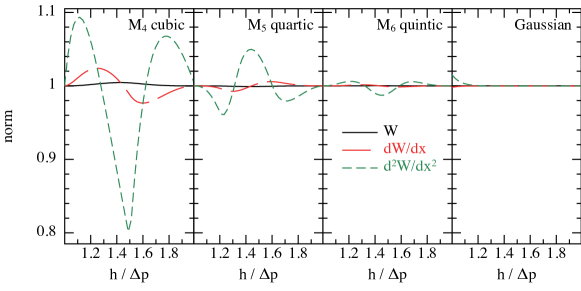
Figure 3: Accuracy with which the normalisation conditions on the kernel, the kernel gradient and the kernel second derivative are computed with fixed $h$ on a one-dimensional line of particles with the $M_{4}$–$M_{6}$ kernels (from left) compared to the Gaussian (right), as a function of the ratio of smoothing length to particle spacing $h/\Delta p$. Bell-shaped kernels with compact support lead to excellent density estimates (solid/black lines), reasonable gradient estimates (long dashed/red lines) but poor second derivative estimates (short dashed/green lines) when a finite number of neighbours are employed.

4.4 First derivatives

From (66) we immediately see that a straightforward improvement to the gradient estimate (51) can be obtained by a simple subtraction of the first error term (i.e., the term in (66) that is present even in the case of a constant function), giving (e.g. Monaghan, 1992)

$$\langle\nabla A_{a}\rangle=\sum_{b}m_{b}\frac{(A_{b}-A_{a})}{\rho_{b}}\nabla_{a}W_{ab},$$ (68)

which, interpreting each term according to (51), is an SPH estimate of

$$\nabla A\approx\langle\nabla A\rangle-A\langle\nabla 1\rangle.$$ (69)

Since the first error term in (66) is removed, the interpolation is exact for constant functions and indeed this is obvious from the form of (68). The interpolation can be made exact for linear functions via a matrix inversion of the second error term in (66), i.e., solving

$$\chi^{\alpha\beta}\frac{\partial A_{a}}{\partial{\bf r}^{\alpha}}=\sum_{b}\frac{m_{b}}{\rho_{b}}(A_{b}-A_{a})\nabla^{\beta}W_{ab},\hskip 28.45274pt\chi^{\alpha\beta}\equiv\sum_{b}\frac{m_{b}}{\rho_{b}}({\bf r}_{b}-{\bf r}_{a})^{\alpha}\nabla^{\beta}W_{ab}.$$ (70)

where $\nabla^{\beta}\equiv\partial/\partial{\bf r}^{\beta}$. This normalisation is somewhat cumbersome in practice, since $\chi$ is a matrix quantity, requiring considerable extra storage (in three dimensions this means storing $3\times 3=9$ extra quantities for each particle) and also since calculation of this term requires prior knowledge of the density.

A similar interpolant for the gradient follows by using

$$\nabla A\approx\frac{1}{\rho}[\langle\nabla(\rho A)\rangle-A\langle\nabla\rho\rangle]=\frac{1}{\rho_{a}}\sum_{b}m_{b}(A_{b}-A_{a})\nabla_{a}W_{ab},$$ (71)

which again is exact for a constant $A$. Expanding $A_{b}$ in a Taylor series, we see that in this case the interpolation of a linear function can be made exact by solving

$$\chi^{\alpha\beta}\frac{\partial A_{a}}{\partial{\bf r}^{\alpha}}=\sum_{b}m_{b}(A_{b}-A_{a})\nabla^{\beta}W_{ab},\hskip 28.45274pt\chi^{\alpha\beta}\equiv\sum_{b}m_{b}({\bf r}_{b}-{\bf r}_{a})^{\alpha}\nabla^{\beta}W_{ab}.$$ (72)

which has some advantages over (70) in that it can be computed without prior knowledge of the density.

However, the gradient operator we derived in the equations of motion (31) does not correspond to any of the above possibilities. This operator is given by

$$\nabla A\approx\rho\left[\frac{A}{\rho^{2}}\langle\nabla\rho\rangle+\langle\nabla\left(\frac{A}{\rho}\right)\rangle\right]=\rho_{a}\sum_{b}m_{b}\left(\frac{A_{a}}{\rho_{a}^{2}}+\frac{A_{b}}{\rho_{b}^{2}}\right)\nabla_{a}W_{ab}.$$ (73)

Expanding $A_{b}$ in a Taylor series about ${\bf r}_{a}$, we have

$$\rho_{a}A_{a}\sum_{b}m_{b}\left(\frac{1}{\rho_{a}^{2}}+\frac{1}{\rho_{b}^{2}}\right)\nabla_{a}W_{ab}+\frac{\partial A_{a}}{\partial{\bf r}^{\alpha}}\rho_{a}\sum_{b}\frac{m_{b}}{\rho_{b}^{2}}({\bf r}_{b}-{\bf r}_{a})^{\alpha}\nabla_{a}W_{ab}+\mathcal{O}(h^{2}),$$ (74)

from which we see that for a constant function the error in (73) is governed by the extent to which

$$\sum_{b}m_{b}\left(\frac{1}{\rho_{a}^{2}}+\frac{1}{\rho_{b}^{2}}\right)\nabla_{a}W_{ab}\approx 0.$$ (75)

Although a simple subtraction of the first term in (74) from the original expression (73) eliminates this error, this would not give the form we derived in Sec. 3.3. Indeed, retaining the exact conservation of momentum requires that such error terms are not eliminated, the consequences of which we will discuss in Sec. 5.

4.5 Generalised first derivative operators

Finally, an infinite variety of gradient operators – of two basic types – can be constructed by noting that

$$\nabla A=\frac{1}{\phi}\left[\nabla(\phi A)-A\nabla\phi\right]\approx\sum_{b}\frac{m_{b}}{\rho_{b}}\frac{\phi_{b}}{\phi_{a}}\left(A_{b}-A_{a}\right)\nabla_{a}W_{ab},$$ (76)

and

$$\nabla A=\phi\left[\frac{A}{\phi^{2}}\nabla\phi+\nabla\left(\frac{A}{\phi}\right)\right]\approx\sum_{b}\frac{m_{b}}{\rho_{b}}\left(\frac{\phi_{b}}{\phi_{a}}A_{a}+\frac{\phi_{a}}{\phi_{b}}A_{b}\right)\nabla_{a}W_{ab},$$ (77)

where $\phi$ is any arbitrary, differentiable scalar quantity defined on the particles. Indeed, for a given $\phi$, the pair of operators defined by (76) and (77) can be shown to form a conjugate pair – and choosing one (e.g. for the density/thermal energy evolution) tends to lead to the other (e.g. in the equations of motion). For example, (68) and (71) correspond to using $\phi=1$ and $\phi=\rho$ respectively in (76), whilst (73) correponds to using $\phi=\rho$ in (77) and arises in the equations of motion because it is the conjugate operator to (71) that arises in the density gradient (57).

Various ‘alternative’ formulations of the SPH equations have been proposed that correspond to a particular choice of $\phi$ (e.g. Hernquist and Katz, 1989; Ritchie and Thomas, 2001; Marri and White, 2003). For example Hernquist and Katz (1989) suggested using an acceleration equation of the form

$$\frac{d{\bf v}}{dt}=-\sum_{b}m_{b}\left(2\frac{\sqrt{P_{a}P_{b}}}{\rho_{a}\rho_{b}}\right)\nabla_{a}W_{ab},$$ (78)

corresponding to the symmetric operator (Eq. 77) with $\phi=\sqrt{P}/\rho$. It can be readily shown that ensuring exact conservation of energy with such a formulation would require using the conjugate operator (i.e., Eq. 76 with $\phi=\sqrt{P}/\rho$) in the thermal energy equation (although it should be noted that simultaneous exact conservation of energy and entropy is not possible with any alternative formulation).

4.6 First derivatives of vector quantities

All of the above discussion applies also to vector derivatives, simply using (53) or (54) in place of (51) and likewise resulting in two basic operators for each type of derivative, given by

$$\langle\nabla\cdot{\bf A}\rangle_{a}\approx\sum_{b}\frac{m_{b}}{\rho_{b}}\frac{\phi_{b}}{\phi_{a}}\left({\bf A}_{b}-{\bf A}_{a}\right)\cdot\nabla_{a}W_{ab};\hskip 28.45274pt\langle\nabla\times{\bf A}\rangle_{a}\approx-\sum_{b}\frac{m_{b}}{\rho_{b}}\frac{\phi_{b}}{\phi_{a}}\left({\bf A}_{b}-{\bf A}_{a}\right)\times\nabla_{a}W_{ab},$$ (79)

and

$$\langle\nabla\cdot{\bf A}\rangle_{a}\approx\sum_{b}\frac{m_{b}}{\rho_{b}}\left(\frac{\phi_{b}}{\phi_{a}}{\bf A}_{a}+\frac{\phi_{a}}{\phi_{b}}{\bf A}_{b}\right)\cdot\nabla_{a}W_{ab};\hskip 28.45274pt\langle\nabla\times{\bf A}\rangle_{a}\approx-\sum_{b}\frac{m_{b}}{\rho_{b}}\left(\frac{\phi_{b}}{\phi_{a}}{\bf A}_{a}+\frac{\phi_{a}}{\phi_{b}}{\bf A}_{b}\right)\times\nabla_{a}W_{ab},$$ (80)

where as previously $\phi$ is an arbitrary (differentiable) scalar quantity. For general vector derivatives written in tensor notation the corresponding expressions are given by

$$\langle\nabla^{j}A^{i}\rangle_{a}\approx\sum_{b}\frac{m_{b}}{\rho_{b}}\frac{\phi_{b}}{\phi_{a}}\left(A^{i}_{b}-A^{i}_{a}\right)\nabla^{j}_{a}W_{ab};\hskip 14.22636pt\textrm{or}\hskip 14.22636pt\langle\nabla^{j}A^{i}\rangle_{a}\approx\sum_{b}\frac{m_{b}}{\rho_{b}}\left(\frac{\phi_{b}}{\phi_{a}}A^{i}_{a}+\frac{\phi_{a}}{\phi_{b}}A^{i}_{b}\right)\nabla^{j}_{a}W_{ab};$$ (81)

These operators form the basic building blocks for formulating quite general SPH equations. Higher order operators can also be constructed for vector derivatives using matrix inversions, similar to (70) and (72).

4.7 Particle methods “the wrong way”: an SPH formulation based on linear errors and exact derivatives

Based on the discussion given in Sec. 4.3–4.6 a straightforward approach would be to simply go ahead and discretise the continuum equations of hydrodynamics (or magnetohydrodynamics) using the most accurate gradient estimates possible. For example employing (68) the hydrodynamic equations of motion $d{\bf v}/dt=-\nabla P/\rho$ could be written in the form

$$\frac{d{\bf v}}{dt}=\sum_{b}m_{b}\left(\frac{P_{a}-P_{b}}{\rho_{a}\rho_{b}}\right)\nabla_{a}W_{ab},$$ (82)

or any of the alternatives offered by choosing $\phi$ appropriately in (76). Indeed such a formulation was originally examined (and discarded) by Morris (1996a, b) but has been recently (re-)proposed by Abel (2010) (the latter author employing $\phi=1/\rho$). We could even proceed to more accurate derivatives using Eqs. (70) or (72) that are exact to linear order. Yet, these operators are clearly different from the equation of motion we derived from the Lagrangian (30), though on the basis of the linear error properties alone (Sec. 4.4) would seem to be a much better choice. On the other hand, it is clear that (82) does not exactly conserve linear (or angular) momentum, nor total energy.

The key difference in approach is that the above analysis tells us about the linear errors, whereas the Hamiltonian formulation tells us about the non-linear properties of the system (i.e., symmetries, conservation and constraints on the behaviour of the global system). These turn out to be crucial for long term stability and accuracy, and we will look at what this means in practice in Sec. 5. That said, “linear errors do not lie”, so it will always be true that – provided the particle distribution is regular – formulations such as (82) or similar will be more accurate for linear or weakly non-linear problems (i.e., those run for a short time and/or not involving strong shocks) and with sufficient resolution can always be made to give accurate results.

Ideally of course, one would want both exact derivatives and exact conservation. In SPH at least, it seems one cannot have both – and to my knowledge this is yet to be convincingly demonstrated by any particle method, though it is perhaps possible using tesselation schemes.

5 Why a bad derivative leads to good derivatives: The importance of local conservation

The paradox we face is that, whilst the Lagrangian derivation gave us valid discretisations of the equations of hydrodynamics, these are not the most accurate discretisations that are possible based on a linear error analysis. Indeed, on the basis of the linear error properties, the gradient estimate derived for the acceleration equation would be a very poor choice of gradient operator, yet it is the only operator which respects all of the symmetry and conservation properties in the Lagrangian.

To understand what these errors mean in practice we can perform a simple thought experiment (which we will also run as a numerical experiment): Consider a distribution of particles in a closed (e.g. periodic) box at constant pressure. In particular, we will consider a uniform random particle distribution. This is the worst-case error scenario, since errors in the interpolation will essentially be Monte-Carlo ($\propto 1/\sqrt{N}$). Now consider what will happen if use one of the more accurate gradient estimators, for example (82). Clearly, since the pressure is constant, there will be no force and hence no particle motion. That is, the force vanishes when the pressure is constant regardless of the particle distribution. If instead we use the Hamiltonian formulation, then the pairwise force between particles is given by

$$\underbrace{-m_{a}m_{b}}_{-ve}\underbrace{\left[\frac{P}{\rho_{a}^{2}}+\frac{P}{\rho_{b}^{2}}\right]}_{+ve}\underbrace{F_{ab}}_{-ve}(\hat{\bf r}_{a}-\hat{\bf r}_{b}).$$ (83)

where we have written the kernel gradient using $\nabla_{a}W_{ab}\equiv\hat{\bf r}_{ab}F_{ab}$. Since for positive definite kernels (Fig. 2) the kernel derivative function is always negative, the overall result – assuming positive pressure – is a positive (that is, repulsive) force between the particles directed along their line of sight. This force will only vanish when the error term (75) becomes zero – that is, when the particles are regular. What this means is that the particles care about their (bad) arrangement and will rearrange themselves until the condition (75) holds, corresponding to a particle distribution that is locally isotropic and regular. This state corresponds to the minimum energy state of the Hamiltonian system – i.e., that which minimises the action (18), and in this state the symmetric gradient estimate (73) is computed with good accuracy (since by definition the motions act to minimise the errors in this estimate). Monaghan (2005) gives some specific examples of this.

In other words, the Hamiltonian SPH formulation – or more generally any formulation which respects local conservation of momentum between particle pairs – contains an intrinsic “re-meshing” procedure and the particles are constrained to remain locally ordered at all times. With an ‘accurate’ but non-conservative pressure estimate the particles are insensitive to their arrangement and can become arbitrarily randomised in the course of a simulation (according to the streamlines of the flow). Thus, methods based on an ‘exact derivatives’ approach (e.g. Dilts, 1999; Maron and Howes, 2003) inevitably require the addition of explicit (and ad-hoc) re-meshing procedures, as the interpolation errors on a randomised particle distribution will be terrible regardless of the order of the interpolation scheme. So in practise the ‘accurate’ gradient estimate will give much less accurate results. This is the paradox of SPH: One deliberately chooses a bad gradient estimate (in the linear errors) in order to obtain a good gradient estimate (because the particles stay regular).

One of the implications of this “intrinsic remeshing” is that not all initial conditions represent stable configurations for the particles. In particular, the cubic lattice – though simple – does not represent a minimum energy state and is only quasi-stable for certain ratios of the smoothing length to the particle separation (Morris, 1996b; Børve et al., 2004). In general, given a small perturbation or sufficient time, the cubic lattice will transition to the more isotropic hexagonal-close-packed lattice arrangement and will do so almost immediately if $h/\Delta p$ is small (e.g. $\eta\lesssim 1.1$).

Figure 4: Settling of an initially random particle distribution due to pairwise conservation of momentum in the pressure gradient. The left and centre columns show the results with the standard (Hamiltonian) SPH method, both without (left) and with (centre) artificial viscosity, after $0.5$ (top) and 10 (bottom) sound crossing times. The right column shows the results when a “relative pressure” formulation is adopted. With a momentum-conserving force the particles are sensitive to their arrangement and will regularise accordingly (left and centre columns), whereas “more accurate” but non-conserving formulations (right) compute gradients that are insensitive to the particle arrangement and thus require explicit re-meshing procedures. Note that although the application of artificial viscosity helps the settling to proceed faster (centre), it is primarily a pressure-driven effect and occurs even if no viscosity is applied (left).

5.1 Example 1: Settling of a random particle distribution

Our first numerical example (using ndspmhd) demonstrates this ‘settling’ in practice. The setup is a two dimensional domain $x,y\in[0,1]$ with periodic boundary conditions. The particles are given an initially uniform thermal energy, density is calculated according to the sum and the pressure is determined using $P=(\gamma-1)\rho u$ with $\gamma=5/3$. The thermal energy is set to give a sound speed $c_{s}=1$, giving $u=0.9$. The end result should therefore be a uniform pressure equilibrium. The particle distributions after 0.5 (top row) and 10 (bottom row) sound crossing times are shown in Fig. 4 using the Hamiltonian SPH formulation (43)–(45) (left and centre columns, without and with artificial viscosity respectively) and the equations of motion computed using a ‘relative pressure’ formulation (specifically, Eq. 76 with $\phi=1/\rho$ as employed by Abel 2010) (right column). With a locally conservative formulation the random initial configuration settles rapidly into a regular particle distribution (left and centre columns), leading in turn to good gradient estimates. This settling occurs even in the absence of an artificial viscosity term (left panels), though adding viscosity does help speed the settling process (centre panels). However, using a “more accurate” but non-conservative gradient estimate there is no regularisation of the particle distribution, leading to poor gradient estimates due to the random nature of the particle distribution. The total energy is also conserved exactly by the SPH formulations, whilst in the relative pressure formulation the total energy grows exponentially.

5.2 Example 2: A 2D shock tube

The other “classic” example of particle settling is the behaviour of SPH particles in a multidimensional shock tube problem, where there is a 1D compression of the particle distribution (e.g. along the x axis). Since the shock induces a highly anisotropic compression – and thus a highly non-preferred particle arrangement – the mutual repulsion of SPH particles will eventually produce a post-shock “remeshing” of the particle distribution, involving transverse motions of the particles. An example is given in Fig. 5, showing the particle distribution at $t=0.1$ in a two dimensional Sod shock tube problem (described further in Sec. 6.3.4) in which the particles were initially placed on two hexagonal close packed lattices upstream and downstream of the shock (initially placed at the origin). The particles can be seen to “break” (at $x\approx 0.14$) from the highly anisotropic compression-induced ‘lines’ at $0.14\lesssim x\lesssim 0.19$, leading to a more isotropic particle distribution further downstream ($x\lesssim 0.12$). This example also illustrates the fact that one inevitably has some motions at the resolution scale that are not related to the physical problem, but related to the implicit “regularisation” of the particle distribution present in locally conservative SPH formulations.

Figure 5: Particle settling in a two dimensional shock tube problem. The particles are initially arranged on hexagonal close packed lattices either side of the shock (top panel). As the shock propagates (bottom panel, showing $t=0.1$) it induces a one dimensional compression in the particles and thus a highly anisotropic particle arrangement, which “remeshes” to a more isotropic arrangement downstream from the shock, involving small motions of particles in the $y-$direction.

5.3 Corollary: Negative pressures and the tensile instability

The corollary of the above is that the particles require a positive pressure in order to remain ordered. If the net pressure (or stress) becomes negative, the net force between a particle pair will become attractive, causing a catastrophic numerical instability. For example, with a pressure gradient of the form

$$\frac{d{\bf v}_{a}}{dt}=-\sum_{b}m_{b}\left(\frac{P_{a}-P_{0}}{\rho_{a}^{2}}+\frac{P_{b}-P_{0}}{\rho_{b}^{2}}\right)\nabla_{a}W_{ab},$$ (84)

the pairwise force will become negative when $P_{0}>P$, and in this situation the particles clump together unphysically. This is known as the ‘tensile instability’ (Monaghan, 2000) and occurs in SPH when a stress tensor is employed that can result in (physically) negative stresses. In particular, this is the case for MHD (Phillips and Monaghan, 1985) and in elastic dynamics (Gray, Monaghan, and Swift, 2001). The occurrence of the tensile instability was one of the main initial difficulties with the development of MHD in SPH and is discussed in detail in Sec. 8.

5.4 The pairing instability: Why one cannot simply use ‘more neighbours’.

Another, more benign, instability in the particle distribution occurs with the cubic spline and other bell-shaped kernels depending on the ratio of smoothing length to particle spacing. This is due to the shape of the kernel gradient term for these kernels (see Fig. 2), and is a consequence of the fact that these kernels are designed to give good density estimates (Sec. 2.2), rather than necessarily being the best choice for calculating gradients. In particular, the kernel gradient in these kernels contains a maximum (negative) value at $r/h\sim 2/3$ and tends to zero at the origin (Fig. 2). This characteristic is desirable for a good density estimate – as it means one is insensitive to a small change in the position of a near neighbour – but means that the mutual repulsive force tends to zero for neighbouring particles placed “within the hump” of the kernel gradient. The net result is that two particles spaced closer than the location of the “hump” in the gradient form a “pair”, eventually falling on top of each other.

Figure 6: The pairing instability in action: The (2D) setup is similar to that shown in Fig. 4 except that the particles are initially placed on a close packed lattice and we use the $M_{4}$ cubic spline kernel with a large ratio of smoothing length to particle spacing (here $\eta=1.5$, corresponding to $\sim 28$ and $100$ neighbours in 2 and 3D respectively). After a few sound crossing times ($t=5$, centre panel) particles form ‘pairs’ which proceed to merge into a locally hexagonal “glass-like” lattice arrangement with almost exactly half the resolution of the initial conditions (right panel, shown after 10 sound crossing times). Although fairly benign – and easily avoided by a sensible choice of $\eta$ – the pairing instability is the main reason one cannot simply “stretch” the cubic spline to large neighbour numbers to achieve convergence. Instead, one should use a kernel with a larger radius of compact support but the same ratio of smoothing length to particle spacing, such as the $M_{5}$ or $M_{6}$ splines.

For the cubic and other B-spline kernels complete merging occurs when $h\gtrsim 1.5\Delta p$ (i.e., $\eta\gtrsim 1.5$ or $\gtrsim 100$ Neighbours in 3D for the cubic spline), corresponding to the placement of the first neighbour “inside the hump”. There is also an intermediate regime $1.225\lesssim\eta\lesssim 1.5$ ($62$–$100$ Neighbours in 3D) where a close-packed or cubic lattice is unstable to pair formation, but where the pairs do not completely merge. These empirical regimes are confirmed by detailed stability analysis of the SPH equations in 2D (Morris, 1996b; Børve et al., 2004) that explicitly show that instability occurs – though with small energies – for large $h/\Delta p$.

Fig. 6 (and our example 3) shows the pairing instability in action: The setup is as for example 1 but with $\eta=1.5$ in the cubic spline kernel instead of $\eta=1.2$ and with particles placed initially on a hexagonal close-packed lattice (an otherwise very stable configuration: left panel). After a few sound crossing times (centre panel) particles begin to form pairs, with these pairs eventually merging completely (right panel) to give a locally hexagonal “glass-like” configuration, but with exactly half the resolution of the initial conditions!

Though fixes have been proposed, none are entirely satisfactory. However, the pairing instability, unlike the tensile instability, is quite benign. For example the density change associated with the transition in Fig. 6 is of order $1\%$ for the cubic spline and $0.1\%$ for the $M_{6}$ quintic – but entails a factor-of-two loss in spatial resolution and is therefore a waste of computational resources. Furthermore, it can be easily avoided by a sensible choice of $\eta$ (we recommend $\eta=1.2$ for the B-spline kernels, corresponding to $N_{neigh}=57.9$ for the cubic spline in 3D). The pairing instability is the main reason one cannot simply “stretch” the cubic spline to large neighbour numbers in order to obtain convergence and demonstrates at least one good reason why $\eta$ (or $N_{neigh}$) should not be regarded as a free parameter in SPH simulations.

6 Second derivatives and dissipation terms in SPH and SPMHD

6.1 The SPH Laplacian

Our remaining “basic” issue regarding both SPH and SPMHD regards the formulation of second derivative terms. As for first derivative terms we can start with the basic summation interpolant (49) and simply take derivatives analytically, e.g.

$$\langle\nabla^{2}A\rangle_{a}\approx\sum_{b}m_{b}\frac{A_{b}}{\rho_{b}}\nabla^{2}_{a}W_{ab}.$$ (86)

Expanding $A_{b}$ in a Taylor series about ${\bf r}_{a}$, we have

$$\sum_{b}m_{b}\frac{A_{b}}{\rho_{b}}\nabla^{2}_{a}W_{ab}=A_{a}\sum_{b}\frac{m_{b}}{\rho_{b}}\nabla^{2}_{a}W_{ab}+\nabla^{\alpha}A_{a}\sum_{b}\frac{m_{b}}{\rho_{b}}{\delta\bf r}^{\alpha}\nabla^{2}_{a}W_{ab}+\frac{1}{2}\nabla^{\alpha}\nabla^{\beta}A_{a}\sum_{b}\frac{m_{b}}{\rho_{b}}{\delta\bf r}^{\alpha}{\delta\bf r}^{\beta}\nabla^{2}_{a}W_{ab}+\ldots.$$ (87)

As previously, we can immediately improve the estimate by subtracting the first error term from both sides, giving an interpolant of the form

$$\sum_{b}\frac{m_{b}}{\rho_{b}}(A_{b}-A_{a})\nabla^{2}_{a}W_{ab}=\nabla^{\alpha}A_{a}\sum_{b}\frac{m_{b}}{\rho_{b}}{\delta\bf r}^{\alpha}\nabla^{2}_{a}W_{ab}+\frac{1}{2}\nabla^{\alpha}\nabla^{\beta}A_{a}\sum_{b}\frac{m_{b}}{\rho_{b}}{\delta\bf r}^{\alpha}{\delta\bf r}^{\beta}\nabla^{2}_{a}W_{ab}+\ldots,$$ (88)

which vanishes when $A$ is constant. However, the accuracy of our second derivative estimate will depend on the remaining error terms in (88), corresponding to the normalisation conditions:

$$\sum_{b}\frac{m_{b}}{\rho_{b}}\delta{\bf r}\nabla^{2}W_{ab}={\bf 0};\hskip 14.22636pt\textrm{and}\hskip 14.22636pt\frac{1}{2}\sum_{b}\frac{m_{b}}{\rho_{b}}\delta{\bf r}^{\alpha}\delta{\bf r}^{\beta}\nabla^{2}W_{ab}=\delta^{\alpha\beta},$$ (89)

such that

$$\nabla^{2}A_{a}\approx\sum_{b}\frac{m_{b}}{\rho_{b}}(A_{b}-A_{a})\nabla^{2}_{a}W_{ab}.$$ (90)

The problem is that the conditions (89) are very poorly satisfied using the second derivative of a compact bell-shaped kernel function (short-dashed/green lines in Fig. 2, showing the second term in 89), since the second derivative changes sign inside the kernel domain (for the cubic spline it is also discontinuous) and must therefore be extremely well sampled in each direction to give accurate results. Thus in practice we require a better functional form – a “second derivative kernel”.

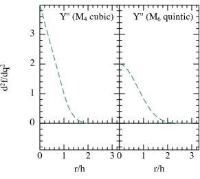
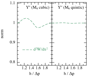
Figure 7: Second derivative kernel functions $Y^{\prime\prime}(q)\equiv-2w^{\prime}(q)/q$ constructed from the first derivatives of the $M_{4}$ cubic and $M_{6}$ quintic kernel functions (left figure, compare to the standard second derivatives shown in Fig. 2), together with the accuracy with which the second derivative normalisation conditions (89) are satisfied for a fixed ratio of $h/\Delta p$ (compare with the standard second derivative functions shown in Fig. 3).

The actual formulation commonly employed derives from early work by Monaghan and first published by Brookshaw (1985), where the SPH Laplacian is written in the form

$$\nabla^{2}A_{a}\approx 2\sum_{b}\frac{m_{b}}{\rho_{b}}(A_{a}-A_{b})\frac{F_{ab}}{|r_{ab}|},$$ (91)

where we use the definition $\nabla_{a}W_{ab}\equiv\hat{\bf r}_{ab}F_{ab}$ such that $F_{ab}$ is the scalar part of the kernel gradient term. Thus in effect we use the first derivative kernel function divided by the particle spacing to give a second derivative. Whilst the interpretation of (91) from the integral representation is in general rather complicated (see, e.g. Español and Revenga, 2003; Jubelgas et al., 2004; Price, 2004; Monaghan, 2005), it can be more easily understood as if we had simply used (90) with a new kernel $Y_{ab}$ instead of $W_{ab}$, defined according to

$$\nabla^{2}Y_{ab}\equiv-\frac{2F_{ab}}{|r_{ab}|}.$$ (92)

The left figure in Fig. 7 shows $Y^{\prime\prime}$ constructed in the above manner from the $M_{4}$ and $M_{6}$ kernel gradients, and may be compared with the standard kernel second derivatives shown in Fig. 2. The right figure shows the normalisation condition (89) for these ‘kernels’. Comparison with Fig. 3 shows that, indeed, the second derivative is much better estimated with kernel second derivative functions that are monotonically decreasing and positive, such as those constructed via (92) from the bell-shaped kernels.

Understanding the Brookshaw (1985) Laplacian as equivalent to (90) with an alternative kernel also helps to interpret more complicated expressions. For example, it is quite straightforward to show that

$$\sum_{b}\frac{m_{b}}{\rho_{b}}(\kappa_{a}+\kappa_{b})(A_{a}-A_{b})\frac{F_{ab}}{|r_{ab}|}\approx\nabla\cdot(\kappa\nabla A),$$ (93)

by writing $-2F_{ab}/|r_{ab}|\equiv\nabla^{2}Y_{ab}$ and interpreting each term via (86). Cleary and Monaghan (1999) proposed an alternative average of the $\kappa$ terms given by

$$\sum_{b}\frac{m_{b}}{\rho_{b}}\frac{4\kappa_{a}\kappa_{b}}{(\kappa_{a}+\kappa_{b})}(A_{a}-A_{b})\frac{F_{ab}}{|r_{ab}|}\approx\nabla\cdot(\kappa\nabla A),$$ (94)

which was formulated to give smooth derivatives when $\kappa$ is discontinuous. The above expression forms the basis of formulations of thermal conductivity in SPH (Cleary and Monaghan, 1999), though has been similarly used to model a wide range of dissipative terms including viscosity (e.g. Cleary et al., 2002; Hu and Adams, 2006), salt diffusion (Monaghan, Huppert, and Worster, 2005) and in an astrophysical context for the treatment of radiation in the Flux-Limited Diffusion approximation (Whitehouse and Bate, 2004; Whitehouse et al., 2005).

6.2 Vector second derivatives

Second derivatives of vector quantities do not quite follow the same analogy as the Laplacian, because in general $\nabla^{i}\nabla^{j}W_{ab}$ involves a mix of the first and second derivatives of the dimensionless kernel function (see appendix A in Price 2010). Thus, the proof is more involved (see Español and Revenga, 2003; Monaghan, 2005, for details), but the basic expressions for vector second derivatives are given by

$$\langle\nabla^{2}{\bf A}\rangle = -2\sum_{b}\frac{m_{b}}{\rho_{b}}({\bf A}_{a}-{\bf A}_{b})\frac{F_{ab}}{|r_{ab}|},$$ (95)

$$\langle\nabla(\nabla\cdot{\bf A})\rangle = -\sum_{b}\frac{m_{b}}{\rho_{b}}\left[(\delta^{k}_{k}+2)({\bf A}_{ab}\cdot\hat{\bf r}_{ab})\hat{\bf r}_{ab}-{\bf A}_{ab}\right]\frac{F_{ab}}{|r_{ab}|},$$ (96)

where $\delta^{k}_{k}\equiv d$ i.e., the number of spatial dimensions. A corollary of the above is that a second derivative computed purely along the line of sight between the particles (e.g. constructed so as to conserve angular momentum) corresponds to

$$-\sum_{b}\frac{m_{b}}{\rho_{b}}({\bf A}_{ab}\cdot\hat{\bf r}_{ab})\frac{F_{ab}}{|r_{ab}|}=\frac{1}{d+2}\nabla(\nabla\cdot{\bf A})+\frac{1}{2(d+2)}\nabla^{2}{\bf A}.$$ (97)

An alternative approach is to calculate vector second derivatives by taking two first derivatives. Although more expensive, this has been the approach adopted in several formulations of physical viscosity, e.g. for SPH modelling of accretion discs (Flebbe et al., 1994; Watkins et al., 1996).

6.3 Artificial dissipation terms in SPH and SPMHD

6.3.1 Interpretation of SPH artificial viscosity terms

This brings us to the formulation and interpretation of artificial dissipation terms in SPH. The ‘standard’ formulation of artificial viscosity is given by (Monaghan, 1992)

$$\left(\frac{d{\bf v}}{dt}\right)_{diss}=-\sum_{b}m_{b}\frac{-\alpha\bar{c}_{s,ab}\mu_{ab}+\beta\mu_{ab}^{2}}{\bar{\rho}_{ab}}\hat{\bf r}_{ab}F_{ab};\hskip 28.45274pt\mu_{ab}=\frac{h{\bf v}_{ab}\cdot{\bf r}_{ab}}{{\bf r}_{ab}+\epsilon\bar{h}_{ab}^{2}},$$ (98)

where barred quantities correspond to an average, i.e., $\bar{\rho}_{ab}=(\rho_{a}+\rho_{b})/2$, $c_{s}$ is the sound speed, $\alpha$ and $\beta$ are dimensionless parameters (typically $\alpha=1$ and $\beta=2$) and $\epsilon\sim 0.01$ is a small parameter to prevent divergences. This form was chosen because it is Galilean invariant, vanishes for rigid body rotation and conserves total linear and angular momentum (Monaghan, 1992). If we neglect the non-linear ($\beta$) term, set $\epsilon=0$ and assume that $c_{s}$, $h$ and $\rho$ are approximately constant over the kernel radius, then using (97) we can directly translate this expression into the continuum form

$$\frac{1}{d+2}\alpha c_{s}h\nabla(\nabla\cdot{\bf v})+\frac{1}{2(d+2)}\alpha c_{s}h\nabla^{2}{\bf v}.$$ (99)

Comparison with the compressible Navier-Stokes equations shows that the artificial viscosity is therefore equivalent to a physical viscosity with shear and bulk coefficients proportional to the resolution length, i.e., (e.g. Artymowicz and Lubow, 1994; Murray, 1996; Monaghan, 2005; Lodato and Price, 2010)

$$\nu\approx\frac{1}{2(d+2)}\alpha c_{s}h;\hskip 28.45274pt\zeta=\frac{5}{3}\nu\approx\frac{5}{6(d+2)}\alpha c_{s}h.$$ (100)

Since for shock-capturing the viscosity is only applied when particles are approaching (${\bf v}_{ab}\cdot{\bf r}_{ab}<0$), in a uniform shear flow – or accretion disc – the viscosity coefficients will be approximately half of these values.

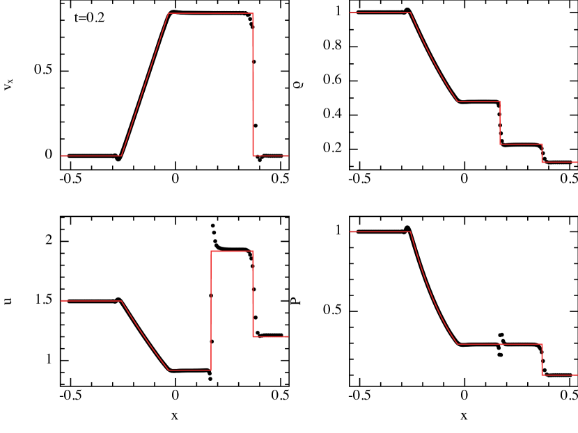
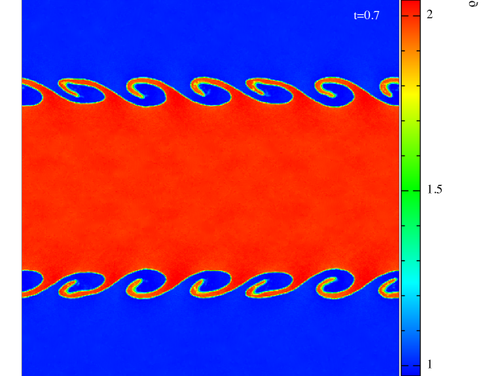
Figure 8: Treatment of discontinuities in SPH: A 1D Sod shock tube problem (left) and 2D Kelvin-Helmholtz instability (right), applying only artificial viscosity terms and with unsmoothed initial conditions. Whilst in the 1D shock tube problem (left panel) the shock is smoothed over several particle spacings by the viscosity term, there are problems at the contact discontinuity causing a ‘blip’ in the pressure. This leads to a suppression of mixing across contact discontinuities in 2D (right panel)

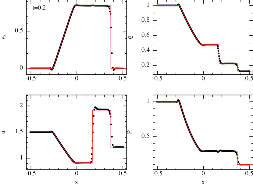
Figure 9: As in Fig. 8 but with artificial conductivity applied as well as artificial viscosity. This smoothes the contact discontinuity, removing the pressure ‘blip’ (left panel) and restoring the mixing in the 2D K-H problem (right panel).

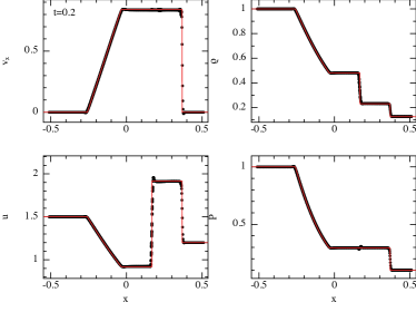
Figure 10: The Sod shock tube in 2D. Using the cubic spline kernel (left panel), there is additional ‘noise’ in the 2D velocity field (compared to 1D, Fig. 9) due to the transverse “remeshing” motions of particles behind the shock front in multidimensions (see Fig. 5). However, this can be quite effectively minimised by using a smoother kernel (right panel, using the $M_{6}$ quintic).

6.3.2 General formulation of dissipative terms in SPH and SPMHD

A more general formulation of dissipative terms was proposed by Monaghan (1997), based on an analogy with Riemann solvers and the need to formulate dissipative terms for ultra-relativistic shocks (Chow and Monaghan, 1997). The general principle is that dissipative terms in the conservative variables involves jumps in those variables (the “left” and “right” states of the Riemann problem), multiplied by eigenvalues that can be interpreted as signal velocities.

For the equations of hydrodynamics the conservative variables are the density, specific momentum and energy ($\rho$, ${\bf v}$ and $e=\frac{1}{2}v^{2}+u$ respectively), and the terms take the form (Monaghan, 1997; Price, 2008)

$$\left(\frac{d{\bf v}_{a}}{dt}\right)_{diss} = \sum_{b}m_{b}\frac{\alpha v_{sig}({\bf v}_{a}-{\bf v}_{b})\cdot\hat{\bf r}_{ab}}{\bar{\rho}_{ab}}\hat{\bf r}_{ab}\overline{F_{ab}},$$ (101)

$$\left(\frac{de_{a}}{dt}\right)_{diss} = \sum_{b}m_{b}\frac{(e^{*}_{a}-e^{*}_{b})}{\bar{\rho}_{ab}}\overline{F_{ab}},$$ (102)

where $e_{a}^{*}=\frac{1}{2}\alpha v_{sig}({\bf v}_{a}\cdot\hat{\bf r}_{ab})^{2}+\alpha_{u}v_{sig}^{u}u_{a}$ refers to an energy including only components along the line of sight joining the particles, $\overline{F_{ab}}\equiv[F_{ab}(h_{a})+F_{ab}(h_{b})]/2$ (equivalent to writing $\bar{F}_{ab}=\hat{\bf r}_{ab}\cdot\overline{\nabla_{a}W_{ab}}$) and $\alpha$ and $\alpha_{u}$ are the dimensionless artificial viscosity and thermal conductivity parameters, respectively. The signal speed $v_{sig}$ refers to the maximum (averaged) signal speed between a particle pair. For hydrodynamics we use

$$v_{sig}=\left\{\begin{array}[]{ll}\frac{1}{2}[c_{s,a}+c_{s,b}-\beta{\bf v}_{ab}\cdot\hat{\bf r}_{ab}];&{\bf v}_{ab}\cdot\hat{\bf r}_{ab}\leq 0;\\ 0;&{\bf v}_{ab}\cdot\hat{\bf r}_{ab}>0.\end{array}\right.$$ (103)

Eq. (101), with the above $v_{sig}$, provides a standard artificial viscosity term similar to (98) (careful expansion shows they differ only by a factor of $h/|r_{ab}|$ and the no-longer-necessary $\epsilon$ term). The dissipation term in the total energy also contains a term involving $(u_{a}-u_{b})$ which acts to smooth jumps in the thermal energy (e.g. at a contact discontinuity). The interpretation of this term is clearer from the contribution to the thermal energy evolution, given by

$$\left(\frac{du}{dt}\right)_{diss}=-\sum_{b}\frac{m_{b}}{\bar{\rho}_{ab}}\left[\frac{1}{2}\alpha v_{sig}({\bf v}_{ab}\cdot\hat{\bf r}_{ab})^{2}+\alpha_{u}v_{sig}^{u}(u_{a}-u_{b})\right]\bar{F}_{ab},$$ (104)

where the second term, from (91), can be directly interpreted as a $\nabla^{2}u$ term. Note that the signal velocity $v_{sig}^{u}$ used in the artificial conductivity does not have to be the same as that used for the viscosity. In particular, Price (2008) proposed using $v_{sig}^{u}=\sqrt{|P_{a}-P_{b}|/\bar{\rho}_{ab}}$ to equalise the pressure across contact discontinuities, whilst Wadsley et al. (2008) proposed a conductivity term equivalent to using $v_{sig}^{u}=|{\bf v}_{ab}\cdot\hat{\bf r}_{ab}|$ (we adopt the former for the tests shown in this paper).

6.3.3 Switches for viscosity terms

One of the key issues in practice is to ensure that sufficient dissipation is applied to discontinuities, but that such dissipation is effectively turned off in smooth parts of the flow by designing appropriate switches. Morris and Monaghan (1997) suggested allowing the parameter $\alpha$ to be individual to each particle, with an evolution equation of the form

$$\frac{d\alpha}{dt}=\mathcal{S}+\frac{\alpha-\alpha_{min}}{\tau};\hskip 28.45274pt\tau=\frac{h}{\sigma c_{s}},$$ (105)

where $\mathcal{S}$ is a source term that grows large at the discontinuity [e.g. $\mathcal{S}=\max(0,-\nabla\cdot{\bf v})$ for shocks], $\tau$ is the decay time, set such that $\alpha$ decays to $\alpha_{min}$ over several smoothing lengths (typically $\sigma=0.1$ and $\alpha_{min}=0.1$). A similar switch can be employed for the thermal conductivity parameter $\alpha_{u}$, with Price and Monaghan (2005) adopting a source term given by $\mathcal{S}_{u}=0.1h\nabla^{2}u$. More sophisticated switches for shock detection are also possible, with a promising recent alternative suggested by Cullen and Dehnen (2010). Directly employing the Riemann solution is another possibility (e.g. Inutsuka, 2002; Cha and Whitworth, 2003).

6.3.4 Examples 4 and 5: One and two dimensional shock tubes, and Kelvin-Helmholtz instabilities

Two specific examples of the dissipative terms in practice are shown in Figs. 8 (applying only viscosity) and 9 (applying artificial viscosity and conductivity), showing the results of a one dimensional Sod shock tube problem (left subfigure) and a two dimensional Kelvin-Helmholtz (K-H) instability problem (right subfigure). The 1D shock tube is setup using a total of 450 particles in $-0.5<x<0.5$ with conditions to the left of the origin given by $[\rho_{L},P_{L},v_{L}]=[1,1,0]$ and to the right by $[\rho_{R},P_{R},v_{R}]=[0.125,0.1,0]$ with $\gamma=5/3$. Importantly, purely discontinuous initial conditions are employed so that the contact discontinuity is not already smoothed. The K-H instability problem is setup with a 2:1 density ratio and equal mass particles, identical to the setup described in Price (2008) and using $512\times 512$ particles in the low density fluid. Whilst shocks are smoothed by the artificial viscosity term (Figs. 8 and 9), with only viscosity the jump in thermal energy at the contact discontinuity is not treated, resulting in a ‘blip’ in the pressure profile (Fig. 8). This manifests in the 2D K-H problem as an ‘artificial surface tension’ effect, caused by the very same kind of pressure blip across the boundary (contact discontinuity) between the dense and the light fluids, suppressing mixing of the two. With conductivity applied (Fig. 9) the pressure is smooth across the contact discontinuity in both problems, which for the K-H problem means that the two fluids mix correctly. The lack of treatment of contact discontinuities in standard SPH codes (i.e., with no artificial conductivity term) explains the discrepancy between grid and SPH results somewhat infamously highlighted by Agertz et al. (2007).

Fig. 10 shows the same shock tube in 2D (as already discussed briefly in Fig. 5). The main difference to 1D is that the “noise” due to the particle resettling behind the shock front is visible (left subfigure). It is often asserted that SPH performs poorly on 2D shocks for this reason, however the noise can be very effectively minimised (at some additional cost) by employing the $M_{6}$ quintic kernel instead of the cubic spline (right subfigure), giving results comparable to the 1D version and illustrating in practice how the higher $M_{n}$ kernels can be used to obtain convergence in SPH.

7 Smoothed Particle Magnetohydrodynamics from a Lagrangian

We can follow the same general approach to constructing an SPMHD algorithm as for hydrodynamics (Sec. 3): Write down the Lagrangian, use appropriate physical constraints and use this to consistently derive the resultant equations of motion.

7.1 MHD Lagrangian

For MHD, the Lagrangian is given by (Price and Monaghan, 2004b)

$$L_{\rm MHD}=\sum_{b}m_{b}\left[\frac{1}{2}v_{b}^{2}-u_{b}(\rho_{b},s_{b})-\frac{1}{2\mu_{0}}\frac{B_{b}^{2}}{\rho_{b}}\right],$$ (106)

corresponding simply to the subtraction of a magnetic energy term from the hydrodynamic verison (Eq. 16). In the continuum limit this corresponds to the standard MHD Lagrangian used by many authors (e.g. Newcomb, 1962; Field, 1986)

$$L_{\rm MHD}=\int\left(\frac{1}{2}\rho v^{2}-\rho u-\frac{1}{2\mu_{0}}B^{2}\right)\mathrm{dV}.$$ (107)

The difference to the hydrodynamic case is that, unlike the thermal energy term, neither the magnetic field ${\bf B}$ nor the change in the magnetic field can be written directly as a function of the particle coordinates, so we cannot straightforwardly employ the Euler-Lagrange equations (21). Instead, we can use the more general form of the variational principle given by $\delta S=\int\delta Ldt=0$ (Sec. 3.2), where from (106) we have

$$\delta L=m_{a}{\bf v}_{a}\cdot\delta{\bf v}_{a}-\sum_{b}m_{b}\left[\left.\frac{\partial u_{b}}{\partial\rho_{b}}\right|_{s}\delta\rho_{b}+\frac{1}{2\mu_{0}}\left(\frac{B_{b}}{\rho_{b}}\right)^{2}\delta\rho_{b}+\frac{1}{\mu_{0}}{\bf B}_{b}\cdot\delta\left(\frac{{\bf B}_{b}}{\rho_{b}}\right)\right],$$ (108)

and the perturbation is with respect to a small change in the particle coordinates $\delta{\bf r}$. So we can derive the equations of motion provided that we are able to express the change in the magnetic field $\delta{\bf B}$ as a function of the change in particle coordinates – equivalent to being able to write down an expression for the Lagrangian time derivative $d{\bf B}/dt$ [or equivalently, $d({\bf B}/\rho)/dt$] since $d/dt\equiv\delta/\delta t$. In other words, in order to derive the SPMHD equations of motion it is necessary to specify not only the density estimate but also the manner in which the magnetic field is evolved.

7.2 SPMHD formulation of the induction equation

Given the induction equation for (ideal) MHD, written in the Lagrangian form

$$\frac{d}{dt}\left(\frac{{\bf B}}{\rho}\right)=\left(\frac{{\bf B}}{\rho}\cdot\nabla\right){\bf v},$$ (109)

and using our general formulations of SPH derivatives given in Sec. 4.6, it is straightforward to write down an SPH version of the form

$$\frac{d}{dt}\left(\frac{{\bf B}_{a}}{\rho_{a}}\right)=-\sum_{b}m_{b}({\bf v}_{a}-{\bf v}_{b})\frac{{\bf B}_{a}}{\Omega_{a}\rho_{a}^{2}}\cdot\nabla W_{ab}(h_{a}),$$ (110)

which is equivalent to using the antisymmetric derivative (81a) with $\phi=\rho$.

7.3 Equations of motion

The perturbations required in (108), from (56) and (110) are therefore given by

$$\delta\rho_{b} = \frac{1}{\Omega_{b}}\sum_{c}m_{c}\left(\delta{\bf r}_{b}-\delta{\bf r}_{c}\right)\cdot\nabla_{b}W_{bc}(h_{b})$$ (111)

$$\delta\left(\frac{{\bf B}_{b}}{\rho_{b}}\right) = -\sum_{c}m_{c}(\delta{\bf r}_{b}-\delta{\bf r}_{c})\frac{{\bf B}_{b}}{\Omega_{b}\rho_{b}^{2}}\cdot\nabla_{b}W_{bc}(h_{b})$$ (112)

giving, from (108) and using (25)

$$\delta S=\int\delta L{\rm dt} = \int\left\{m_{a}{\bf v}_{a}\cdot\delta{\bf v}_{a}-\sum_{b}m_{b}\left[\left(\frac{P_{b}+\frac{1}{2}B_{b}^{2}/\mu_{0}}{\Omega_{b}\rho_{b}^{2}}\right)\sum_{c}m_{c}\nabla_{b}W_{bc}(h_{b})(\delta_{ba}-\delta_{ca})\right]\cdot{\delta{\bf r}_{a}}\right.$$ (113)

$$\phantom{\int\{}+\left.\sum_{b}m_{b}\left[\frac{{\bf B}_{b}}{\mu_{0}}\sum_{c}m_{c}\frac{{\bf B}_{b}}{\Omega_{b}\rho_{b}^{2}}\cdot\nabla_{b}W_{bc}(h_{b})(\delta_{ba}-\delta_{ca})\right]\cdot{\delta{\bf r}_{a}}\right\}{\rm dt}=0,$$

where $\delta_{ba}\equiv\delta{\bf r}_{b}/\delta{\bf r}_{a}$. Integrating the velocity term by parts, simplifying the double summations using the Kronecker deltas and the antisymmetry of the kernel gradient, and assuming the perturbations $\delta{\bf r}_{a}$ are arbitrary, we find that the SPMHD equations of motion are given by

$$\frac{d{\bf v}_{a}}{dt} = -\sum_{b}m_{b}\left[\frac{P_{a}+\frac{1}{2\mu_{0}}B_{a}^{2}}{\Omega_{a}\rho_{a}^{2}}\nabla_{a}W_{ab}(h_{a})+\frac{P_{b}+\frac{1}{2\mu_{0}}B_{b}^{2}}{\Omega_{b}\rho_{b}^{2}}\nabla_{a}W_{ab}(h_{b})\right]$$ (114)

$$+\frac{1}{\mu_{0}}\sum_{b}m_{b}\left[\frac{{\bf B}_{a}({\bf B}_{a}\cdot\nabla_{a}W_{ab}(h_{a}))}{\Omega_{a}\rho_{a}^{2}}+\frac{{\bf B}_{b}({\bf B}_{b}\cdot\nabla_{a}W_{ab}(h_{b}))}{\Omega_{b}\rho_{b}^{2}}\right].$$

In tensor notation these can be written more compactly in the form

$$\frac{dv^{i}_{a}}{dt}=\sum_{b}m_{b}\left[\frac{S^{ij}_{a}}{\Omega_{a}\rho_{a}^{2}}\nabla^{j}_{a}W_{ab}(h_{a})+\frac{S^{ij}_{b}}{\Omega_{b}\rho_{b}^{2}}\nabla^{j}_{a}W_{ab}(h_{b})\right],$$ (115)

where $S^{ij}$ is the MHD stress tensor, defined according to

$$S^{ij}\equiv-\left(P+\frac{1}{2\mu_{0}}B^{2}\right)\delta^{ij}+\frac{1}{\mu_{0}}B^{i}B^{j}.$$ (116)

As for the hydrodynamic case (Sec. 3) it is readily seen that the equations of motion conserve linear momentum exactly, due to the pairwise symmetry in the force. However, the MHD equations, unlike their hydrodynamic counterparts, do not exactly conserve angular momentum, since the perturbation to the magnetic field, (112) – and hence the anisotropic force term derived from it – is not invariant to rotations. It is interesting to note that the anisotropic magnetic force term in (114) derives entirely from the numerical representation of the induction equation (110), whilst the isotropic term derives purely from the magnetic energy term in the Lagrangian and the density perturbation (111).

7.4 Energy equation

The evolution equations for thermal energy and entropy – in the absence of dissipation – are identical to their hydrodynamic counterparts. The total energy evolution can be deduced from the Hamiltonian as in Sec. 3.4.2. The corresponding expression for MHD is given by

$$\frac{dE}{dt}=\sum_{a}m_{a}\left[{\bf v}_{a}\cdot\frac{d{\bf v}_{a}}{dt}+\frac{du_{a}}{dt}+\frac{1}{2}\frac{B_{a}^{2}}{\rho_{a}^{2}}\frac{d\rho_{a}}{dt}+{\bf B}_{a}\cdot\frac{d}{dt}\left(\frac{{\bf B}_{a}}{\rho_{a}}\right)\right].$$ (117)

Using (115), (35), (56) and (110), it can be shown that the total energy evolves according to

$$\frac{dE}{dt}=\sum_{a}m_{a}\sum_{b}m_{b}\left[\left(\frac{S^{ij}}{\Omega\rho^{2}}\right)_{a}v^{i}_{b}\nabla^{j}_{a}W_{ab}(h_{a})+\left(\frac{S^{ij}}{\Omega\rho^{2}}\right)_{b}v^{i}_{a}\nabla^{j}_{a}W_{ab}(h_{b})\right]=0,$$ (118)

and is thus also conserved exactly. This further implies an evolution equation for the specific energy $e\equiv\frac{1}{2}v^{2}+u+\frac{1}{2\mu_{0}}B^{2}/\rho$ of the form

$$\frac{de_{a}}{dt}=\sum_{b}m_{b}\left[\left(\frac{S^{ij}}{\Omega\rho^{2}}\right)_{a}v^{i}_{b}\nabla^{j}_{a}W_{ab}(h_{a})+\left(\frac{S^{ij}}{\Omega\rho^{2}}\right)_{b}v^{i}_{a}\nabla^{j}_{a}W_{ab}(h_{b})\right],$$ (119)

7.5 Interpretation of the Hamiltonian SPMHD equations

Having used the SPH forms of the continuity and induction equations in the form

$$\frac{d\rho}{dt} = -\rho\frac{\partial v^{i}}{\partial x^{i}},$$ (120)

$$\frac{d}{dt}\left(\frac{B^{i}}{\rho}\right) = -\frac{B^{j}}{\rho}\frac{\partial v^{i}}{\partial x^{j}},$$ (121)

it is straightforward to show (using 55) that our expressions (115) and (119) derived above are SPH representations of the MHD acceleration and energy equations in the form

$$\frac{dv^{i}}{dt} = \frac{1}{\rho}\frac{\partial S^{ij}}{\partial x^{j}},$$ (122)

$$\frac{de}{dt} = \frac{\partial(v^{i}S^{ij})}{\partial x^{j}},$$ (123)

where $S^{ij}$ is the MHD stress tensor given by (116). That we have explicitly used the induction equation to derive the equations of motion and energy is useful to our later discussion regarding what is a consistent formulation of monopole terms in the MHD equations (Sec. 10.1).

7.5.1 MHD Example 1: Advection of a current loop

Our first MHD example demonstrates that some problems that prove very difficult for Eulerian schemes are almost trivial in a Lagrangian scheme such as SPMHD. The problem involves the advection of a loop of current across the computational domain, was introduced by Gardiner and Stone (2005) to test their Athena MHD code and presents a challenging problem for grid-based MHD schemes. The setup used here is identical to that in Rosswog and Price (2007) and we refer the reader to that paper (or the ndspmhd setup file) for full details. The current loop itself is given by the vector potential $A_{z}=A_{0}(R-\sqrt{x^{2}+y^{2}})$, with $A_{0}$ set to give a weak field (plasma $\beta$ of $2\times 10^{6}$) (here we compute and evolve the magnetic field, ${\bf B}$). All particles in the domain ($-1<x<1$, $-0.5<y<0.5$) are given a constant initial velocity along the box diagonal, with the magnitude set such that $t=1$ represents one crossing of the domain. The results are shown in Fig. 11, at $t=0$ (left panel) and after $1000$ (this is not a misprint!) crossings of the computational domain (right panel). In the absence of the explicit addition of resistivity terms, there is no change in the current or the magnetic energy and the advection is computed exactly.

Figure 11: Advection of a current loop across a 2D domain. Magnetic field lines are shown at $t=0$ (left panel) and after 1000 crossings of the computational domain (right panel). In the absence of the explicit addition of resistivity terms, there is no change in the magnetic field and the advection is computed exactly in SPMHD, irrespective of the direction of propagation, numerical resolution or advection velocity.

8 The tensile instability in MHD

The rather large caveat to using the equations of motion derived in Sec. 7.3 is that in MHD the total stress can become negative, meaning that the force between particles can become attractive rather than repulsive and the equations will be unstable to the tensile instability discussed in Sec. 5.3. The regime of instability is evident if we consider the force in just one spatial dimension (and at constant h), given by

$$\frac{dv^{x}_{a}}{dt}=-\sum_{b}m_{b}\left[\frac{P_{a}-\frac{1}{2\mu_{0}}B_{x}^{2}}{\rho_{a}^{2}}+\frac{P_{b}-\frac{1}{2\mu_{0}}B_{x}^{2}}{\rho_{b}^{2}}\right]\frac{dW_{ab}}{dx},$$ (124)

so the force will become attractive (along the field lines) when $\frac{1}{2}B^{2}/\mu_{0}>P$, i.e., when magnetic pressure exceeds gas pressure. A more detailed stability analysis (e.g. Phillips and Monaghan, 1985; Morris, 1996b, a; Børve et al., 2004) confirms that this is also the criterion for instability in more than one spatial dimension. Thus, whilst for particular applications that remain in the regime where magnetic pressure is smaller than gas pressure it is possible to use the conservative formulation (e.g. Dolag, Bartelmann, and Lesch, 1999), in most cases stabilising the tensile instability is the first and most basic requirement for a stable SPMHD algorithm.

The physical reason for the MHD instability is that the momentum-conserving force corresponds to

$$\frac{d{\bf v}}{dt}=\frac{\nabla\cdot{\bf S}}{\rho}\equiv-\frac{\nabla P}{\rho}+\frac{(\nabla\times{\bf B})\times{\bf B}}{\mu_{0}\rho}+\frac{{\bf B}\nabla\cdot{\bf B}}{\mu_{0}\rho},$$ (125)

which differs from equations of motion written in terms of the Lorentz force (where ${\bf J}=\nabla\times{\bf B}/\mu_{0}$),

$$\frac{d{\bf v}}{dt}=-\frac{\nabla P}{\rho}+\frac{{\bf J}\times{\bf B}}{\rho},$$ (126)

by the “monopole term” in (125). This term gives a force directed along the magnetic field and proportional to the (numerically non-zero) divergence of the magnetic field, and is the source of the instability in the conservative formulation if it cannot be counteracted by pressure. As a result, Eq. 126 was used as the basis of a number of early SPMHD formulations in which the force was simply computed using standard curl operators such as (54) or (79) (e.g. Meglicki, 1995; Byleveld and Pongracic, 1996; Cerqueira and de Gouveia Dal Pino, 2001; Hosking and Whitworth, 2004). However, the poor conservation properties of such formulations means that MHD shocks are not well captured.

Dealing with such ‘source terms’ is not an issue unique to SPMHD and requires careful consideration in all numerical MHD formulations (see Sec. 10.1). Of course, $\nabla\cdot{\bf B}=0$ should be zero physically due to the non-existence of magnetic monopoles in the Universe, so both (126) and (125) are valid in the continuum limit. The problem is that the divergence term is not exactly zero numerically – so one is forced to make a choice. As noted by Tóth (2000), it is also not a simple matter of enforcing the $\nabla\cdot{\bf B}=0$ constraint in some way, since what is necessary to achieve a force that is both conservative and exactly perpendicular to ${\bf B}$ is to constrain $\nabla\cdot{\bf B}$ to be zero in the discretisation that the term appears in the force equation. In SPMHD this is equivalent to requiring both exact derivatives and exact conservation which, as discussed in Sec. 4.7, does not appear to be possible.

8.1 Fix 1: subtract a constant from the stress

The original paper by Phillips and Monaghan (1985) proposed a simple fix involving a prior sweep over the particles to find the maximum (negative) stress, which would then simply be subtracted (as a constant) from the stress in the equations of motion, giving

$$\frac{dv^{i}_{a}}{dt}=\sum_{b}m_{b}\left[\frac{S^{ij}_{a}-S^{ij}_{max}}{\Omega_{a}\rho_{a}^{2}}\nabla^{j}_{a}W_{ab}(h_{a})+\frac{S^{ij}_{b}-S^{ij}_{max}}{\Omega_{b}\rho_{b}^{2}}\nabla^{j}_{a}W_{ab}(h_{b})\right],$$ (127)

which conserves momentum but not total energy. The caveats are that there is a computational cost involved to compute $S^{ij}_{max}$ and if this term is large it can lead to unphysical effects in the simulation. On the other hand, this is a simple technique that removes the instability and has relatively few side effects provided the correction is small. It is particularly useful if, for example, the simulation is dominated by large (constant) external stresses, whereby explicitly subtracting the external component of the stress (e.g. due to an externally imposed magnetic field) can serve to stabilise the formulation.

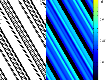
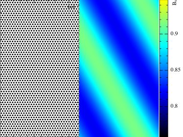
Figure 12: The tensile instability in SPMHD: The figures show the particle distribution (left panel in each figure) and $x$-component of the magnetic field (right panel in each figure) in the 2.5D circularly polarized Alfvén wave test using the (unstable) conservative SPMHD force (left figure) and with a stable formulation (right figure), shown after 1 wave crossing time. Untreated, the MHD tensile instability results in a catastrophic clumping of particles along the magnetic field lines (left figure) which proceeds to destroy the calculation. Physically, it can be attributed to non-zero divergence terms in the conservative form of the MHD force, and can be stabilised by explicitly subtracting the unphysical ‘source term’ (right figure).

8.2 Fix 2: use a more accurate but non-conservative gradient estimate in the anisotropic force

Morris (1996b) proposed a compromise approach whereby one retains conservative form in the isotropic part of the force, but adopts a more accurate but non-conservative derivative estimate (that vanishes when the stress is constant) in the anisotropic term. Adapted for variable smoothing lengths, the resultant force is given by (Price and Monaghan, 2005; Price, 2010)

$$\frac{dv_{a}^{i}}{dt}=-\sum_{b}m_{b}\left[\frac{P_{a}+\frac{1}{2\mu_{0}}B^{2}_{a}}{\Omega_{a}\rho_{a}^{2}}\nabla^{i}_{a}W_{ab}(h_{a})+\frac{P_{b}+\frac{1}{2\mu_{0}}B^{2}_{b}}{\Omega_{b}\rho_{b}^{2}}\nabla_{a}^{i}W_{ab}(h_{b})\right]+\frac{1}{\mu_{0}}\sum_{b}m_{b}\frac{(B_{i}B_{j})_{b}-(B_{i}B_{j})_{a}}{\rho_{a}\rho_{b}}\overline{\nabla^{j}W}_{ab},$$ (128)

where $\overline{\nabla W_{ab}}\equiv[\nabla W_{ab}(h_{a})+\nabla W_{ab}(h_{b})]/2$. The ‘Morris approach’ does not exactly conserve momentum or total energy, but the errors due to non-conservation are in practice quite small even on strong shock tube problems (see Price, 2004). Note, however, that retaining local conservation in the isotropic term is important for the reasons discussed in Sec. 5 and also in order to obtain the correct jump conditions on MHD shocks. The caveat to this approach is that the remaining non-conservation of momentum can become problematic, especially in simulations run for a long time period, where secular effects can accumulate and cause a loss of symmetry, and that it cannot be turned “off” in the otherwise stable weak-field regime.

8.3 Fix 3: subtract the unphysical source term

Børve et al. (2001) suggested an approach whereby conservation form is retained, but the monopole source term is explicitly subtracted. Extending their expression to incorporate variable smoothing length terms, the corrected equations of motion are given by

$$\frac{dv^{i}_{a}}{dt}=\sum_{b}m_{b}\left[\frac{S^{ij}_{a}}{\Omega_{a}\rho_{a}^{2}}\nabla^{j}_{a}W_{ab}(h_{a})+\frac{S^{ij}_{b}}{\Omega_{b}\rho_{b}^{2}}\nabla^{j}_{a}W_{ab}(h_{b})\right]-\hat{B}_{a}^{i}\sum_{b}m_{b}\left[\frac{B^{j}_{a}}{\Omega_{a}\rho_{a}^{2}}\nabla^{j}_{a}W_{ab}(h_{a})+\frac{B^{j}_{b}}{\Omega_{b}\rho_{b}^{2}}\nabla^{j}_{a}W_{ab}(h_{b})\right].$$ (129)

The corrective term with $\hat{B}^{i}_{a}={B}^{i}_{a}$ is equivalent to the source term added to the momentum equation in the eight-wave Riemann solver (Powell et al., 1999) – with the key point from an SPH standpoint being that the discretisation used for the correction term is identical to that in which the divergence term occurs in the force equation. Børve et al. (2004) also showed that it is not necessarily required to always choose $\hat{B}^{i}_{a}=B^{i}_{a}$ in order to achieve stability, showing in particular that $\hat{B}^{i}_{a}=\frac{1}{2}B^{i}_{a}$ is sufficient. Børve, Omang, and Trulsen (2006) give a more general method for setting $\hat{B}^{i}$ such that – amongst other things – no correction is applied when the gas pressure exceeds the magnetic pressure (we refer the reader to their paper for more details). Whilst adding the correction term violates exact conservation of momentum and energy, it does so only insofar as the divergence term in (129) is non-zero. Like the Morris approach, (129) is a good general method for removing the tensile instability in SPMHD – but has the advantage of being able to be switched off in the regime where the conservative formulation is stable.

8.4 Other methods

Finally, other methods have been proposed for dealing with the tensile instability in other physical problems, such as elastic dynamics. In particular Monaghan (2000) suggested explicitly adding a short range repulsive force between particles to counteract the unphysical attractive force, similar to what would occur in atoms. Price and Monaghan (2004a) initially applied this approach to the MHD equations and it was shown by Price (2004) to be equivalent to a modification of the kernel gradient in the anisotropic part of the MHD force (the second term in Eq. 114). However it proved problematic in highly compressible calculations where the smoothing lengths could vary dramatically (leading to a difficulty in defining “short range”) and at large negative stress was found to result in large errors in the numerical sound speed (see Price, 2004). It was therefore abandoned by Price and Monaghan (2005) in favour of either the Morris or Børve et al. (2001) approaches.

8.4.1 MHD Example 2: Circularly polarized Alfvén wave in 2.5D

An example of the tensile instability in practice is shown in Fig. 12, which shows the particle distribution (left panels in each figure) and $x$-component of the magnetic field (right panels in each figure) in the 2.5D circularly polarized Alfvén wave test from Tóth (2000). The initial conditions (Tóth, 2000; Price and Monaghan, 2005) are $\rho=1$, $P=0.1$, $v_{\parallel}=0$, $B_{\parallel}=1$, $v_{\perp}=B_{\perp}=0.1\sin{(2\pi r_{\parallel})}$ and $v_{z}=B_{z}=0.1\cos{(2\pi r_{\parallel})}$ with $\gamma=5/3$ (where $r_{\parallel}=x\cos{\theta}+y\sin{\theta}$), with the wave vector directed at an angle of $\theta=30^{\circ}$ with respect to the $x$-axis in the computational domain $0<x<1/\cos{\theta}$, $0<y<1/\sin{\theta}$ with periodic boundary conditions.

Using a conservative SPMHD formulation (left figure, shown at $t=1$) whole lines of particles can be seen to have attracted each other in the direction of $B_{\parallel}$, which proceeds to destroy the calculation at later times. With either the Morris or Børve et al. approach (right figure, also shown at $t=1$) the particle arrangement – and hence the wave – is stable and propagates correctly.

9 Dissipation terms and shocks in SPMHD

The second important issue for SPMHD is the formulation of dissipation terms appropriate for MHD shocks. We can follow the same general principle as in Sec. 6.3.2, starting with (102) as the basic equation, except that in MHD the energy variable is given by

$$e^{*}_{a}=\frac{1}{2}\alpha v_{sig}({\bf v}_{a}\cdot\hat{\bf r}_{ab})^{2}+\alpha_{u}v_{sig}^{u}u_{a}+\alpha_{B}v_{sig}^{B}\frac{B^{2}_{a}}{2\mu_{0}\bar{\rho}_{ab}},$$ (130)

and the signal velocity in the kinetic energy term is generalised to

$$v_{sig}=\left\{\begin{array}[]{ll}\frac{1}{2}[v_{a}+v_{b}-\beta{\bf v}_{ab}\cdot\hat{\bf r}_{ab}];&{\bf v}_{ab}\cdot\hat{\bf r}_{ab}\leq 0;\\ 0;&{\bf v}_{ab}\cdot\hat{\bf r}_{ab}>0,\end{array}\right.$$ (131)

where $v$ is the fastest wave speed for MHD (i.e., the fast MHD mode), given by

$$v_{a}=\frac{1}{\sqrt{2}}\left[\left(c_{s,a}^{2}+\frac{B^{2}_{a}}{\mu_{0}\rho_{a}}\right)+\sqrt{\left(c_{s,a}^{2}+\frac{B^{2}_{a}}{\mu_{0}\rho_{a}}\right)^{2}-4\frac{c_{s,a}^{2}({\bf B}_{a}\cdot\hat{\bf r}_{ab})^{2}}{\mu_{0}\rho_{a}}}\right]^{1/2}.$$ (132)

The key constraint in deriving dissipative terms in the other equations is that the contribution to the entropy from the dissipative terms in the total energy equation must be positive definite in order to satisfy the second law of thermodynamics. For the kinetic energy term this is satisfied provided a term is added to the acceleration equation (i.e., Eq. 101), giving a positive definite contribution to the thermal energy (Eq. 104). It may also be shown that the thermal energy term results in a positive definite contribution to the entropy (Appendix B of Price and Monaghan 2004a). For the magnetic energy term, positivity means that the overall dissipative contribution to the thermal energy equation is given by

$$\left(\frac{du}{dt}\right)_{diss}=-\sum_{b}\frac{m_{b}}{\bar{\rho}_{ab}}\left[\frac{1}{2}\alpha v_{sig}({\bf v}_{a}-{\bf v}_{b})^{2}+\alpha_{u}v_{sig}^{u}(u_{a}-u_{b})+v_{sig}^{B}\frac{\alpha_{B}}{2\mu_{0}\bar{\rho}_{ab}}({\bf B}_{a}-{\bf B}_{b})^{2}\right]\overline{F_{ab}},$$ (133)

which is positive definite because $F_{ab}$ is negative definite (Fig. 2) and the terms inside the brackets are positive. Using (133), we can deduce the term which must arise in the induction equation using

$$\frac{d}{dt}\left(\frac{B^{2}}{2\mu_{0}\rho}\right)_{diss}=\left(\frac{de}{dt}\right)_{diss}-{\bf v}\cdot\left(\frac{d{\bf v}}{dt}\right)_{diss}-\left(\frac{du}{dt}\right)_{diss},$$ (134)

giving a term in the induction equation of the form

$$\left(\frac{d{\bf B}_{a}}{dt}\right)_{diss}=\rho_{a}\sum_{b}m_{b}\frac{\alpha_{B}v^{B}_{sig}}{\bar{\rho}_{ab}^{2}}\left({\bf B}_{a}-{\bf B}_{b}\right)\bar{F}_{ab},$$ (135)

or, evolving ${\bf B}/\rho$,

$$\frac{d}{dt}\left(\frac{{\bf B}_{a}}{\rho_{a}}\right)_{diss}=\sum_{b}m_{b}\frac{\alpha_{B}v^{B}_{sig}}{\bar{\rho}_{ab}^{2}}\left({\bf B}_{a}-{\bf B}_{b}\right)\bar{F}_{ab}.$$ (136)

The interpretation of this term is straightforward using (95): We have derived an artificial resistivity term

$$\left(\frac{d{\bf B}_{a}}{dt}\right)_{diss}=\eta_{M}\nabla^{2}{\bf B}_{a};\hskip 28.45274pt\eta_{M}\approx\frac{1}{2}\alpha_{B}v_{sig}^{B}|r_{ab}|.$$ (137)

For the artificial resistivity it is also better to use a signal velocity that differs from the one used in the viscosity. A simple choice (used in ndspmhd) is to use an averaged Alfvén speed, e.g.

$$v_{sig}^{B}=\frac{1}{2}\sqrt{v_{A,a}^{2}+v_{A,b}^{2}};\hskip 28.45274ptv_{A}^{2}=\frac{B^{2}}{\mu_{0}\rho}.$$ (138)

Price and Monaghan (2004a, 2005) also show how an artificial resistivity can be derived that uses only components of the magnetic field perpendicular to the line of sight. However, Price and Monaghan (2005) found that the version using the jump in total energy (Eqs. 130, 135) performed better in practice. The parameter $\alpha_{B}$ can also be evolved using a switch similar to (105), where Price and Monaghan (2005) suggest a source term of the form

$$\mathcal{S}=\mathrm{max}\left(\frac{|\nabla\times{\bf B}|}{\sqrt{\mu_{0}\rho}},\frac{|\nabla\cdot{\bf B}|}{\sqrt{\mu_{0}\rho}}\right).$$ (139)

Note that artificial thermal conductivity and resistivity should in general be applied regardless of whether or not the particle pair is approaching or receding.

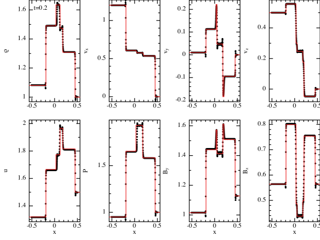
Figure 13: A “1.75D” MHD shock tube problem, showing the formation of 7 discontinuities: A slow, Alfvén and fast wave propagating in each direction, plus the contact discontinuity. Capture of all of these discontinuities requires the application of artificial viscosity, thermal conductivity and resistivity to treat jumps in $v$, $u$ and $B$ respectively. The $M_{4}$ cubic spline kernel has been used.

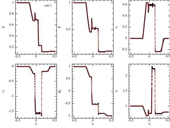
Figure 14: The Brio-Wu MHD shock tube problem in 2D, computed using $800\times 24$ particles and the $M_{6}$ quintic kernel. With the quintic, results comparable to the 1D solution can be obtained. The numerical solution from Balsara (1998) is given by the solid (red) line. All particles are plotted.

9.1 MHD Example 3: shock tube problems in MHD

The application of specific dissipative terms for shock-capturing is illustrated in Fig. 13, which shows a “1.75D” MHD shock tube problem (i.e., 1D but with 3D magnetic and velocity fields) from Ryu and Jones (1995), using 800 particles and the standard $M_{4}$ cubic spline kernel. The setup is $(\rho,P,v_{x},v_{y},v_{z},B_{y},B_{z})=[1.08,0.95,1.2,0.01,0.5,3.6/(4\pi)^{1/2},2/(4\pi)^{1/2}]$ for $x<0$, whilst for $x\geq 0$ we have $(\rho,P,v_{x},v_{y},v_{z},B_{y},B_{z})=[1,1,0,0,0,4/(4\pi)^{1/2},2/(4\pi)^{1/2}]$, with $B_{x}=2/(4\pi)^{1/2}$ and $\gamma=5/3$. The main point is that this shows all 7 possible discontinuities in MHD: Three waves (slow, Alfvén and fast modes) propagating in each direction, plus the contact discontinuity. Since each requires treatment, we require artificial viscosity, thermal conductivity and resistivity to treat the jumps in velocity, thermal energy and magnetic field respectively.

Fig. 14 shows a 2D version of the Brio and Wu (1988) shock tube test, considered a standard test for MHD codes (e.g. Stone et al., 1992; Dai and Woodward, 1994; Ryu and Jones, 1995; Balsara, 1998), using $800\times 24$ particles and the $M_{6}$ quintic kernel. Initially $(\rho,P,v_{x},v_{y},B_{y})=[1,1,0,0,1]$ for $x<0$, with $(\rho,P,v_{x},v_{y},B_{y})=[0.125,0.1,0,0,-1]$ for $x\geq 0$ with $B_{x}=0.75$ everywhere and $\gamma=2.0$. Profiles of all SPMHD particles are plotted at $t=0.1$ whilst the numerical solution from Balsara (1998) is given by the solid (red) line. The solution is comparable to that achievable in 1D (e.g. Rosswog and Price, 2007) – at this resolution the only noticeable deviation from the Balsara solution is the slight mismatch in thermal energy at $x\approx 0.15$–$0.3$, a result of the low spatial resolution (10$\times$ lower than in the $x<0$ region) in this low density region.

10 The divergence constraint in SPMHD

The third major issue, common to all numerical MHD codes, is how to enforce the $\nabla\cdot{\bf B}=0$ constraint. The problem arises because the constraint occurs only as an initial condition in the MHD equations, since from the induction equation we have

$$\frac{\partial{\bf B}}{\partial t}=-\nabla\times({\bf v}\times{\bf B});\hskip 28.45274pt\frac{\partial}{\partial t}\left(\nabla\cdot{\bf B}\right)=0,$$ (140)

The problem is that the truncation error in the numerical solution means that such a condition cannot be maintained indefinitely. What to do about it falls into three general approaches: “ignore”, “clean” or “prevent” the numerical growth of monopole terms. We will discuss each of these in the context of SPMHD, but first turn to the issue of formulating consistent equations given that $\nabla\cdot{\bf B}\neq 0$.

10.1 $\nabla\cdot{\bf B}\neq 0$: Monopole terms in the evolution equations

We have already touched on the ‘source terms’ issue in the context of the tensile instability in SPMHD, which arises from the fact that the MHD force written as the divergence of a stress tensor differs from the exactly-perpendicular-to-B Lorentz force by a term proportional to $\nabla\cdot{\bf B}$ – and that this term does not vanish even in the trivial case of 1D where $B_{x}=const$. A similar issue arises in the induction equation (140), which in “conservative form” is given by

$$\frac{\partial{\bf B}}{\partial t}=\nabla\cdot({\bf v}{\bf B}-{\bf B}{\bf v})=-({\bf v}\cdot\nabla){\bf B}+({\bf B}\cdot\nabla){\bf v}-{\bf B}(\nabla\cdot{\bf v})+{\bf v}(\nabla\cdot{\bf B}),$$ (141)

identical to (140), and conserving the volume integral of the flux $\int{\bf B}{\rm dV}$. However, if the monopole term ${\bf v}(\nabla\cdot{\bf B})$ is neglected, then we have (using the Lagrangian time derivative)

$$\frac{d{\bf B}}{dt}=({\bf B}\cdot\nabla){\bf v}-{\bf B}(\nabla\cdot{\bf v}),$$ (142)

taking the divergence of which shows that the monopoles evolve according to an equation similar to the continuity equation for density

$$\frac{\partial}{\partial t}\left(\nabla\cdot{\bf B}\right)+\nabla\cdot({\bf v}\nabla\cdot{\bf B}),$$ (143)

meaning that the volume integral $\int_{\rm V}(\nabla\cdot{\bf B}){\rm dV}$, and by Green’s theorem the surface integral of the flux, $\oint_{S}{\bf B}\cdot{\rm d{\bf S}}$ is conserved. So adopting (142) represents a ‘monopole conserving’ form of the induction equation, such that the surface flux integral will be conserved even if the divergence errors are non-zero. On the basis of this idea Powell et al. (1999) suggested the 8-wave formulation, with the induction equation given by (142) and the momentum and energy equations given by

$$\frac{dv^{i}}{dt} = \frac{1}{\rho}\frac{\partial S^{ij}}{\partial x^{j}}-\frac{B^{i}}{\rho}\frac{\partial B^{j}}{\partial x^{j}},$$ (144)

$$\frac{de}{dt} = \frac{1}{\rho}\frac{\partial(v_{i}S^{ij})}{\partial x^{j}}-\frac{v_{i}B^{i}}{\rho}\frac{\partial B^{j}}{\partial x^{j}},$$ (145)

However, Janhunen (2000) and Dellar (2001) have strongly argued that a consistent formulation in the presence of monopoles, whilst adopting (142) instead of (140), should nevertheless still conserve linear (but not angular) momentum and energy. For SPMHD we have already proved that this is the case because we derived the momentum-conserving force (115) from the surface-flux-and-monopole conserving induction equation (109). This is a somewhat moot point in practice though, since we require the subtraction of the source term in the momentum equation anyway in order to stabilise the tensile instability (Sec. 8.3), giving essentially the 8-wave formulation.

10.2 $\nabla\cdot{\bf B}\approx 0$: The “ignore” approach

The simplest approach to the divergence constraint is to do nothing at all. That is, simply monitor the divergence error and “trust” the simulations if it remains small. In SPMHD it is usual to monitor the divergence error using the dimensionless quantity

$$\frac{h\nabla\cdot{\bf B}}{|B|},$$ (146)

typically hoping that it remains smaller than a few percent. For a number of problems, including many of the test problems shown in this paper, this approach works surprisingly well. There is also the question of what one means by the “divergence error”, since (146) can be computed using a variety of operators (Sec. 4.4) and the ‘stencil’ in which one measures divergence changes in SPH as soon as one changes the particle positions. However there are clearly many problems where this approach is not sufficient.

10.3 $\nabla\cdot{\bf B}\to 0$: The “clean” approach

Divergence cleaning in SPMHD also faces the problem of defining what $\nabla\cdot{\bf B}=0$ actually means. Clearly from a stability point of view it would be desirable for the divergence to be zero in the discretisation in which it enters the force equation, but we have already seen that this is not possible even in 1D because the conservative SPH derivative does not vanish for constant functions. However, it may be hoped that cleaning in a particular discretisation will at least produce solenoidal fields to the order of the truncation error [i.e., $\mathcal{O}(h^{2})$]. Approaches to divergence cleaning fall into three general categories based on the solution to an elliptic, parabolic or hyperbolic partial differential equation.

10.3.1 Elliptic cleaning

Elliptic cleaning corresponds to using projection methods: Solving either for a correction term,

$${\bf B}={\bf B}^{*}-\nabla\phi;\hskip 28.45274pt\nabla^{2}\phi=\nabla\cdot{\bf B}^{*},$$ (147)

or alternatively for the physical (solenoidal) component of the field,

$${\bf B}=\nabla\times{\bf A};\hskip 28.45274pt\nabla^{2}{\bf A}=-\nabla\times{\bf B}^{*}.$$ (148)

SPH methods for both of the above have been discussed by Price and Monaghan (2005). The main issue is that, if one simply uses the Green’s function solution – analogous to the computation of gravitational forces – with the source function computed with a chosen div or curl operator, the projection is only approximate (that is, the Poisson equation is not discretely satisfied). For 3D simulations with particles on individual timesteps, it is also impractical and highly inefficient to compute a global projection every $n$ timesteps.

10.3.2 Parabolic cleaning

A parabolic approach corresponds to adding a $\nabla\cdot{\bf B}$ diffusion term to the induction equation, i.e.,

$$\left(\frac{d{\bf B}}{dt}\right)_{clean}=\nabla\cdot(\eta_{c}\nabla\cdot{\bf B}).$$ (149)

Having formulated our artificial dissipative terms using the jump in total magnetic energy (130) means that the artificial resistivity already contains a term of this form (see 137), so applying artificial resistivity (with a switch that responds to the divergence, Eq. 139) corresponds to a form of parabolic divergence cleaning. This is partly why the “ignore” approach is not as bad as it sounds, and has successfully used for a number of problems (e.g. Dolag and Stasyszyn, 2009; Kotarba et al., 2010; Bürzle et al., 2010).

10.3.3 Hyperbolic/parabolic cleaning

Dedner et al. (2002) suggested a hyperbolic cleaning method for the MHD equations, given by

$$\frac{d{\bf B}}{dt}=-{\bf B}(\nabla\cdot{\bf v})+({\bf B}\cdot\nabla){\bf v}-\nabla\psi,$$ (150)

where $\psi$ is an additional variable that evolves according to (Price and Monaghan, 2005)

$$\frac{d\psi}{dt}=-c_{h}^{2}(\nabla\cdot{\bf B})-\frac{\psi}{\tau},$$ (151)

where for SPH it is natural to use $c_{h}\equiv v_{sig}$ and $\tau\equiv\alpha_{h}h/v_{sig}$ where $\alpha_{h}\in[0,1]$ is a dimensionless parameter. The first term in (151) corresponds to hyperbolic propagation of the “divergence wave” (at speed $c_{h}$), whilst $\psi/\tau$ is a parabolic decay term (with decay time $\tau$). This can be shown combining the equations (assuming ${\bf v}=const$) to yield a wave equation,

$$\frac{1}{c_{h}^{2}}\frac{\partial^{2}\psi}{\partial t^{2}}-\nabla^{2}\psi+\tau\frac{\partial\psi}{\partial t}=0.$$ (152)

As reported by Price and Monaghan (2005) and others (e.g. Mignone and Tzeferacos, 2010), the original Dedner et al. (2002) formulation contained a parameter that is not dimensionless, but that is equivalent to the wavelength of critical damping $\lambda_{c}$ in the parabolic decay term (evident by writing $\tau\equiv\lambda_{c}/c_{h}$ in the above). Indeed, Price and Monaghan (2005) found that whilst using (150)-(151) could be effective at cleaning well-resolved divergence errors ($\lambda_{c}\gg h$), it was found to have little or no effect when used in “real” problems (where $\lambda_{c}\sim h$), giving at most a factor of $\sim 2$ reduction in $\nabla\cdot{\bf B}_{\rm max}$. It was also found that a poor choice of parameters could increase the divergence error substantially via constructive interference of divergence waves.

More recently Stasyszyn & Dolag (following Dolag and Stasyszyn, 2009) report better success using this method, by two adaptations: i) accounting for the magnetic energy dissipation in the energy equation, and ii) implementation of a limiter to control the amount by which the magnetic field can change in a single timestep (Dolag 2010, priv. commun.). Nevertheless, it does not appear that the method is being used on real problems (e.g. Kotarba et al., 2010), suggesting that it remains ineffective.

10.4 $\nabla\cdot{\bf B}=0$: The “prevent” approach

The third approach is to try to ‘prevent’ divergence errors altogether by formulating the MHD equations such that $\nabla\cdot{\bf B}=0$ is satisfied by construction. Unfortunately, the approach most successfully adopted in grid based schemes – the constrained transport method (Evans and Hawley, 1988; Gardiner and Stone, 2005) – cannot be directly applied in an SPH context because it requires the computation of surface rather than volume integrals.

10.4.1 Euler potentials

Perhaps the closest to a ‘constrained transport’ approach in SPMHD is the formulation in terms of Euler potentials (Stern, 1970, 1976) (also referred to as “Clebsch variables”, e.g. by Phillips and Monaghan 1985), $\alpha_{E}$ and $\beta_{E}$, where the magnetic field is expressed as

$${\bf B}=\nabla\alpha_{E}\times\nabla\beta_{E}.$$ (153)

Taking the divergence shows that $\nabla\cdot{\bf B}=0$ is satisfied by construction. A further advantage is that for ideal MHD, the induction equation (109) becomes simply

$$\frac{d\alpha_{E}}{dt}=0,\hskip 14.22636pt\frac{d\beta_{E}}{dt}=0,$$ (154)

which corresponds physically to the advection of magnetic field lines by Lagrangian particles (Stern, 1966). That is, the Euler potentials reflect the physical fact that the field lines are ‘frozen’ to the fluid in ideal MHD and are therefore a natural description for a Lagrangian scheme. For SPH it is straightforward to write down expressions for (153) using any of our standard first derivative operators (Sec. 4.4) and to simply use the resultant ${\bf B}$ in the SPMHD equations of motion – though this will give only approximate conservation of energy, see Price 2010. However, in order to capture shocks, some dissipation in the magnetic field is required. For this reason Price and Bate (2007) and Rosswog and Price (2007) introduced dissipation terms of the form

$$\left(\frac{d\alpha_{E}^{a}}{dt}\right)_{diss}=\sum_{b}\frac{m_{b}}{\bar{\rho}_{ab}}\alpha_{B}v^{B}_{sig}\left(\alpha_{E}^{a}-\alpha_{E}^{b}\right)\overline{F_{ab}};\hskip 14.22636pt\left(\frac{d\beta_{E}^{a}}{dt}\right)_{diss}=\sum_{b}\frac{m_{b}}{\bar{\rho}_{ab}}\alpha_{B}v^{B}_{sig}\left(\beta_{E}^{a}-\beta_{E}^{b}\right)\overline{F_{ab}},$$ (155)

corresponding to the continuum equations (assuming $\eta_{\rm M}\approx const$)

$$\frac{d\alpha_{E}}{dt}\approx\eta_{\rm M}\nabla^{2}\alpha;\hskip 28.45274pt\frac{d\beta_{E}}{dt}=\eta_{\rm M}\nabla^{2}\beta,$$ (156)

where $\eta_{\rm M}$ is given by (137). However it is clear that this is not a consistent formulation of (physical) resistivity for the Euler potentials, since we have neglected mixed terms that are of comparable magnitude to those in (156) (e.g. Brandenburg, 2010). It is also difficult to ensure that the contribution to the entropy is positive definite, although Price (2010) shows how the latter requirement can be achieved for the vector potential, and similar formulations should be used in place of (155) for the Euler potentials.

Nevertheless, the control of the divergence errors means that the Euler potentials have found successful application to a range of problems (e.g. Price and Bate, 2007; Dobbs and Price, 2008; Kotarba et al., 2009), most notably in star formation (e.g. Price and Bate, 2007, 2008, 2009) since one is able to form stars in the presence of magnetic fields without blow-up of the numerical solution due to divergence errors. The caveat is that the Euler potentials do not capture the full physics of MHD, since the Helicity ${\bf A}\cdot{\bf B}$ is identically zero, meaning that topologically non-trivial fields cannot be represented (or by corollary, created during a simulation) using (153)–(154). For example, the Euler potentials cannot be used to follow multiple complete windings of a magnetic field in a rotating fluid, a corollary of the fact that the potentials are simply advected by the particles (Eq. 154), so reconstruction of the field via (153) requires a one-to-one mapping between the initial and final particle positions. These restrictions are easily demonstrated by simple test problems (Brandenburg, 2010) and mean in practice that one is limited to studying problems with initially simple field geometries, and that important field winding processes (i.e., any dynamo action) are missed. On the other hand, it may be possible to formulate a more general Euler potentials description without such limitations.

10.4.2 The vector potential

Another possibility for a divergence-free formulation without the restrictions of the Euler potentials is to simply employ the vector potential ${\bf B}=\nabla\times{\bf A}$ directly. Indeed in 2D they are exactly equivalent, since for a 2D field $\alpha_{E}\equiv A_{z}(x,y)$ and $\beta_{E}\equiv z$. The main disadvantage of the vector potential in 3D is that the evolution equation is complicated and requires an appropriate gauge choice. For example, setting the scalar potential $\phi={\bf v}\cdot{\bf A}$ one can obtain a Galilean-invariant evolution equation for ${\bf A}$ of the form (Price, 2010)

$$\frac{d{\bf A}}{dt}=-{\bf A}\times(\nabla\times{\bf v})-({\bf A}\cdot\nabla){\bf v}+{\bf v}\times{\bf B}_{ext}=-A^{j}\nabla v^{j}+{\bf v}\times{\bf B}_{ext}.$$ (157)

Using this, one can proceed to derive an SPMHD algorithm for the vector potential from the Lagrangian (106). In particular, Price (2010) shows that by writing the curl according to

$${\bf B}_{a}=(\nabla\times{\bf A})_{a}+{\bf B}_{ext}=\frac{1}{\rho_{a}}\sum_{b}m_{b}({\bf A}_{a}-{\bf A}_{b})\times\nabla_{a}W_{ab}+{\bf B}_{ext},$$ (158)

the effective evolution equation for ${\bf B}$ is given by

$$\frac{d{\bf B}_{a}}{dt} = \frac{1}{\rho_{a}}\sum_{b}m_{b}\left({\bf A}_{a}-{\bf A}_{b}\right)\times[({\bf v}_{a}-{\bf v}_{b})\cdot\nabla]\nabla_{a}W_{ab}$$ (159)

$$+ \frac{1}{\rho_{a}}\sum_{b}m_{b}\left(\frac{d{\bf A}_{a}}{dt}-\frac{d{\bf A}_{b}}{dt}\right)\times\nabla_{a}W_{ab}-\frac{{\bf B}_{int}}{\rho_{a}}\frac{d\rho_{a}}{dt}.$$

Thus, writing the evolution equation for ${\bf A}$, (157), in the form

$$\frac{d{\bf A}_{a}}{dt}=\frac{A^{a}_{j}}{\rho_{a}}\sum_{b}m_{b}(v^{j}_{a}-v^{j}_{b})\nabla_{a}W_{ab}+({\bf v}\times{\bf B}_{ext})_{a},$$ (160)

one can self-consistently derive equations of motion for the vector potential from (108) by writing the perturbation to $\delta{\bf B}$ in terms of $\delta{\bf A}$ using (159) and $\delta{\bf A}$ in terms of $\delta{\bf r}$ using (160), giving

$$\frac{d{\bf v}_{a}}{dt} = -\sum_{b}m_{b}\left(\frac{P_{a}-\frac{3}{2\mu_{0}}B_{a}^{2}}{\rho_{a}^{2}}+\frac{P_{b}-\frac{3}{2\mu_{0}}B_{b}^{2}}{\rho_{b}^{2}}\right)\nabla_{a}W_{ab}$$ (161)

$$- \frac{1}{\mu_{0}}\sum_{b}m_{b}\left\{\left(\frac{{\bf B}_{a}}{\rho_{a}^{2}}+\frac{{\bf B}_{b}}{\rho_{b}^{2}}\right)\cdot\left[({\bf A}_{a}-{\bf A}_{b})\times\nabla\right]\right\}\nabla_{a}W_{ab}$$

$$- \frac{2}{\mu_{0}}\sum_{b}m_{b}\left(\frac{{\bf B}_{a}}{\rho_{a}^{2}}+\frac{{\bf B}_{b}}{\rho_{b}^{2}}\right)\cdot{\bf B}_{ext}\nabla_{a}W_{ab}+\frac{1}{\mu_{0}}\sum_{b}m_{b}\left(\frac{{\bf B}_{a}}{\rho_{a}^{2}}+\frac{{\bf B}_{b}}{\rho_{b}^{2}}\right){\bf B}_{ext}\cdot\nabla_{a}W_{ab}$$

$$- \sum_{b}m_{b}\left[\frac{{\bf A}_{a}}{\rho_{a}^{2}}{\bf J}_{a}\cdot\nabla_{a}W_{ab}+\frac{{\bf A}_{b}}{\rho_{b}^{2}}{\bf J}_{b}\cdot\nabla_{a}W_{ab}\right],$$

where ${\bf J}$ the magnetic current is computed using the symmetric curl operator (the conjugate to 158),

$${\bf J}_{a}\equiv\frac{\left(\nabla\times{\bf B}\right)_{a}}{\mu_{0}}\equiv-\frac{\rho_{a}}{\mu_{0}}\sum_{b}m_{b}\left[\frac{{\bf B}_{a}}{\rho_{a}^{2}}+\frac{{\bf B}_{b}}{\rho_{b}^{2}}\right]\times\nabla_{a}W_{ab}.$$ (162)

The proof that the above equations do indeed translate into an continuum expression of the conservative MHD equations, as well as a more general version taking full account of smoothing length gradient terms is given by Price (2010). However, the major flaw, from simple inspection of (161), is that the isotropic (first) term will give a negative pressure – and thus the tensile instability – whenever $3B^{2}/(2\mu_{0})>P$, a much more restrictive regime than for the usual SPMHD equations (see Sec. 8). This is verified in test problems, but unlike the standard SPMHD instability, proves difficult to stabilise without significantly affecting the solution. A second instability was also found to arise purely due to the evolution of ${\bf A}$ according to (157), resulting in unconstrained growth of vector potential components, most likely related to the need to explicitly enforce a gauge condition alongside the evolution of the vector potential. Price (2010) therefore concluded that using the vector potential was not a viable approach for SPMHD.

11 Summary

In summary, we have given an overview of SPH methodology, starting with the density estimate as the basis of all SPH formulations (Sec. 2) and showing how the equations of motion and energy can be self-consistently derived from the density estimate using a variational principle (Sec. 3). Kernel interpolation theory has been introduced mainly as a way of interpreting the SPH equations, and we have discussed how linear error analysis can be used to construct more accurate and very general derivative operators (Sec. 4). In Sec. 5 the importance of local conservation was highlighted with respect to maintaining a regular particle distribution and thus accurate derivatives, giving us an understanding of how the tensile instability arises in SPMHD and why one should be careful in setting the ratio of smoothing length to particle spacing. Second derivatives in SPH were discussed in Sec. 6, mainly as a way of formulating dissipative terms necessary to capture shocks and other kinds of discontinuities. In the second half of the paper, we have shown how SPMHD, like SPH, can also be formulated from a variational principle (Sec. 7) and have addressed the three main issues with regards to the accuracy of SPMHD: The tensile instability (Sec. 8), the formulation of shock-capturing dissipation terms (Sec. 9) and the enforcement of the divergence-free condition on the magnetic field (Sec. 10). Finally, this paper marks the public release of the ndspmhd SPH/SPMHD code that can be used to test and verify all of the ideas and methods that have been discussed.

References

- Abel (2010) Abel, T., Mar. 2010. rpSPH: a much improved Smoothed Particle Hydrodynamics Algorithm. arXiv:1003.0937.
- Agertz et al. (2007) Agertz, O., Moore, B., Stadel, J., Potter, D., Miniati, F., Read, J., Mayer, L., Gawryszczak, A., Kravtsov, A., Nordlund, Å., Pearce, F., Quilis, V., Rudd, D., Springel, V., Stone, J., Tasker, E., Teyssier, R., Wadsley, J., Walder, R., Sep. 2007. Fundamental differences between SPH and grid methods. MNRAS 380, 963–978.
- Artymowicz and Lubow (1994) Artymowicz, P., Lubow, S. H., Feb. 1994. Dynamics of binary-disk interaction. 1: Resonances and disk gap sizes. ApJ 421, 651–667.
- Balsara (1998) Balsara, D. S., May 1998. Total Variation Diminishing Scheme for Adiabatic and Isothermal Magnetohydrodynamics. ApJS 116, 133.
- Benz (1990) Benz, W., 1990. Smoothed Particle Hydrodynamics - A review. In: Buchler, J. R. (Ed.), The numerical modelling of nonlinear stellar pulsations. Kluwer, pp. 269–288.
- Børve et al. (2001) Børve, S., Omang, M., Trulsen, J., Nov. 2001. Regularized Smoothed Particle Hydrodynamics: A New Approach to Simulating Magnetohydrodynamic Shocks. ApJ 561, 82–93.
- Børve et al. (2004) Børve, S., Omang, M., Trulsen, J., Aug. 2004. Two-dimensional MHD Smoothed Particle Hydrodynamics Stability Analysis. ApJS 153, 447–462.
- Børve et al. (2006) Børve, S., Omang, M., Trulsen, J., Dec. 2006. Multidimensional MHD Shock Tests of Regularized Smoothed Particle Hydrodynamics. ApJ 652, 1306–1317.
- Brandenburg (2010) Brandenburg, A., Jan. 2010. Magnetic field evolution in simulations with Euler potentials. MNRAS 401, 347–354.
- Brio and Wu (1988) Brio, M., Wu, C. C., Apr. 1988. An upwind differencing scheme for the equations of ideal magnetohydrodynamics. J. Comp. Phys. 75, 400–422.
- Brookshaw (1985) Brookshaw, L., 1985. A method of calculating radiative heat diffusion in particle simulations. Proceedings of the Astronomical Society of Australia 6, 207–210.
- Bürzle et al. (2010) Bürzle, F., Clark, P. C., Stasyszyn, F., Greif, T., Dolag, K., Klessen, R. S., Nielaba, P., Aug. 2010. Protostellar collapse and fragmentation using an MHD GADGET. arXiv:1008.3790.
- Byleveld and Pongracic (1996) Byleveld, S. E., Pongracic, H., Jan. 1996. The influence of magnetic fields on star formation. PASA 13, 71–74.
- Cerqueira and de Gouveia Dal Pino (2001) Cerqueira, A. H., de Gouveia Dal Pino, E. M., Oct. 2001. Three-dimensional Magnetohydrodynamic Simulations of Radiatively Cooling, Pulsed Jets. ApJ 560, 779–791.
- Cha and Whitworth (2003) Cha, S.-H., Whitworth, A. P., Mar. 2003. Implementations and tests of Godunov-type particle hydrodynamics. MNRAS 340, 73–90.
- Chow and Monaghan (1997) Chow, E., Monaghan, J. J., 1997. Ultrarelativistic SPH. J. Comp. Phys. 134, 296–305.
- Cleary et al. (2002) Cleary, P., Ha, J., Alguine, V., Nguyen, T., 2002. Flow modelling in casting processes. Appl. Math. Modelling 26 (2), 171 – 190.
- Cleary and Monaghan (1999) Cleary, P. W., Monaghan, J. J., Jan. 1999. Conduction Modelling Using Smoothed Particle Hydrodynamics. J. Comp. Phys. 148, 227–264.
- Couchman (1991) Couchman, H. M. P., Feb. 1991. Mesh-refined P3M - A fast adaptive N-body algorithm. ApJL 368, L23–L26.
- Cullen and Dehnen (2010) Cullen, L., Dehnen, W., Jul. 2010. Inviscid smoothed particle hydrodynamics. MNRAS, 1126.
- Cummins and Rudman (1999) Cummins, S. J., Rudman, M., Jul. 1999. An SPH Projection Method. J. Comp. Phys. 152, 584–607.
- Dai and Woodward (1994) Dai, W., Woodward, P. R., Dec. 1994. Extension of the Piecewise Parabolic Method to Multidimensional Ideal Magnetohydrodynamics. J. Comp. Phys. 115, 485–514.
- Dedner et al. (2002) Dedner, A., Kemm, F., Kröner, D., Munz, C.-D., Schnitzer, T., Wesenberg, M., Jan. 2002. Hyperbolic Divergence Cleaning for the MHD Equations. J. Comp. Phys. 175, 645–673.
- Dehnen (2001) Dehnen, W., Jun. 2001. Towards optimal softening in three-dimensional N-body codes - I. Minimizing the force error. MNRAS 324, 273–291.
- Dellar (2001) Dellar, P. J., Sep. 2001. A Note on Magnetic Monopoles and the One-Dimensional MHD Riemann Problem. J. Comp. Phys. 172, 392–398.
- Dilts (1999) Dilts, G., 1999. Moving-least-squares-particle hydrodynamics - i. consistency and stability. Int. J. Num. Meth. Eng. 44 (8), 1115–1155.
- Dobbs and Price (2008) Dobbs, C. L., Price, D. J., Jan. 2008. Magnetic fields and the dynamics of spiral galaxies. MNRAS 383, 497–512.
- Dolag et al. (1999) Dolag, K., Bartelmann, M., Lesch, H., Aug. 1999. SPH simulations of magnetic fields in galaxy clusters. A&A 348, 351–363.
- Dolag and Stasyszyn (2009) Dolag, K., Stasyszyn, F., Oct. 2009. An MHD GADGET for cosmological simulations. MNRAS 398, 1678–1697.
- Eckart (1960) Eckart, C., May 1960. Variation Principles of Hydrodynamics. Physics of Fluids 3, 421–427.
- Español and Revenga (2003) Español, P., Revenga, M., Feb. 2003. Smoothed dissipative particle dynamics. Phys. Rev. E 67 (2), 026705.
- Evans and Hawley (1988) Evans, C. R., Hawley, J. F., Sep. 1988. Simulation of magnetohydrodynamic flows - A constrained transport method. ApJ 332, 659–677.
- Field (1986) Field, G., 1986. Magnetic helicity in astrophysics. In: Epstein, R., Feldman, W. (Eds.), AIP Conf. Proc. 144: Magnetospheric Phenomena in Astrophysics. pp. 324–341.
- Flebbe et al. (1994) Flebbe, O., Muenzel, S., Herold, H., Riffert, H., Ruder, H., Aug. 1994. Smoothed Particle Hydrodynamics: Physical viscosity and the simulation of accretion disks. ApJ 431, 754–760.
- Fulk and Quinn (1996) Fulk, D. A., Quinn, D. W., Jun. 1996. An Analysis of 1-D Smoothed Particle Hydrodynamics Kernels. J. Comp. Phys. 126, 165–180.
- Gardiner and Stone (2005) Gardiner, T. A., Stone, J. M., May 2005. An unsplit Godunov method for ideal MHD via constrained transport. J. Comp. Phys. 205, 509–539.
- Gingold and Monaghan (1977) Gingold, R. A., Monaghan, J. J., Nov. 1977. Smoothed particle hydrodynamics - Theory and application to non-spherical stars. MNRAS 181, 375–389.
- Gray et al. (2001) Gray, J., Monaghan, J. J., Swift, R. P., Oct. 2001. SPH elastic dynamics. Computer methods in applied mechanics and engineering 190, 6641–6662.
- Harlow and Welch (1965) Harlow, F. H., Welch, J. E., Dec. 1965. Numerical Calculation of Time-Dependent Viscous Incompressible Flow of Fluid with Free Surface. Physics of Fluids 8, 2182–2189.
- Hernquist and Katz (1989) Hernquist, L., Katz, N., Jun. 1989. TREESPH - A unification of SPH with the hierarchical tree method. ApJS 70, 419–446.
- Heß and Springel (2010) Heß, S., Springel, V., Aug. 2010. Particle hydrodynamics with tessellation techniques. MNRAS 406, 2289–2311.
- Hockney and Eastwood (1981) Hockney, R. W., Eastwood, J. W., 1981. Computer Simulation Using Particles. New York: McGraw-Hill, 1981.
- Hosking and Whitworth (2004) Hosking, J. G., Whitworth, A. P., Jan. 2004. Modelling ambipolar diffusion with two-fluid smoothed particle hydrodynamics. MNRAS 347, 994–1000.
- Hu and Adams (2006) Hu, X. Y., Adams, N. A., Apr. 2006. A multi-phase SPH method for macroscopic and mesoscopic flows. J. Comp. Phys. 213, 844–861.
- Inutsuka (2002) Inutsuka, S., Jun. 2002. Reformulation of Smoothed Particle Hydrodynamics with Riemann Solver. J. Comp. Phys. 179, 238–267.
- Janhunen (2000) Janhunen, P., May 2000. A Positive Conservative Method for Magnetohydrodynamics Based on HLL and Roe Methods. J. Comp. Phys. 160, 649–661.
- Jubelgas et al. (2004) Jubelgas, M., Springel, V., Dolag, K., Apr. 2004. Thermal conduction in cosmological SPH simulations. MNRAS preprint, 000.
- Kats (2001) Kats, A. V., May 2001. Variational principle and canonical variables in hydrodynamics with discontinuities. Physica D, 459–474.
- Kotarba et al. (2010) Kotarba, H., Karl, S. J., Naab, T., Johansson, P. H., Dolag, K., Lesch, H., Stasyszyn, F. A., Jun. 2010. Simulating Magnetic Fields in the Antennae Galaxies. ApJ 716, 1438–1452.
- Kotarba et al. (2009) Kotarba, H., Lesch, H., Dolag, K., Naab, T., Johansson, P. H., Stasyszyn, F. A., Aug. 2009. Magnetic field structure due to the global velocity field in spiral galaxies. MNRAS 397, 733–747.
- Kulasegaram et al. (2004) Kulasegaram, S., Bonet, J., Lewis, R. W., Profit, M., 2004. A variational formulation based contact algorithm for rigid boundaries in two-dimensional SPH applications. Comp. Mech. 33, 316–325.
- Lodato and Price (2010) Lodato, G., Price, D. J., Jun. 2010. On the diffusive propagation of warps in thin accretion discs. MNRAS 405, 1212–1226.
- Lucy (1977) Lucy, L. B., Dec. 1977. A numerical approach to the testing of the fission hypothesis. Astron. J. 82, 1013–1024.
- Maron and Howes (2003) Maron, J. L., Howes, G. G., Sep. 2003. Gradient Particle Magnetohydrodynamics: A Lagrangian Particle Code for Astrophysical Magnetohydrodynamics. ApJ 595, 564–572.
- Marri and White (2003) Marri, S., White, S. D. M., Oct. 2003. Smoothed particle hydrodynamics for galaxy-formation simulations: improved treatments of multiphase gas, of star formation and of supernovae feedback. MNRAS 345, 561–574.
- Meglicki (1995) Meglicki, Z., 1995. Analysis and applications of Smoothed Particle Magnetohydrodynamics. Ph.D. thesis, Australian National University.
- Mignone and Tzeferacos (2010) Mignone, A., Tzeferacos, P., Mar. 2010. A second-order unsplit Godunov scheme for cell-centered MHD: The CTU-GLM scheme. J. Comp. Phys. 229, 2117–2138.
- Monaghan (1985) Monaghan, J. J., Sep. 1985. Extrapolating B. Splines for Interpolation. J. Comp. Phys. 60, 253.
- Monaghan (1992) Monaghan, J. J., 1992. Smoothed particle hydrodynamics. Ann. Rev. Astron. Astrophys. 30, 543–574.
- Monaghan (1997) Monaghan, J. J., Sep. 1997. SPH and Riemann Solvers. J. Comp. Phys. 136, 298–307.
- Monaghan (2000) Monaghan, J. J., Apr. 2000. SPH without a Tensile Instability. J. Comp. Phys. 159, 290–311.
- Monaghan (2002) Monaghan, J. J., Sep. 2002. SPH compressible turbulence. MNRAS 335, 843–852.
- Monaghan (2004) Monaghan, J. J., Mar. 2004. Energy transfer in a particle model. J. Turb. 5, 12.
- Monaghan (2005) Monaghan, J. J., 2005. Smoothed particle hydrodynamics. Rep. Prog. Phys. 68 (8), 1703–1759.
- Monaghan et al. (2005) Monaghan, J. J., Huppert, H. E., Worster, M. G., Jul. 2005. Solidification using smoothed particle hydrodynamics. J. Comp. Phys. 206, 684–705.
- Monaghan and Lattanzio (1985) Monaghan, J. J., Lattanzio, J. C., Aug. 1985. A refined particle method for astrophysical problems. A&A 149, 135–143.
- Monaghan and Price (2001) Monaghan, J. J., Price, D. J., Dec. 2001. Variational principles for relativistic smoothed particle hydrodynamics. MNRAS 328, 381–392.
- Morris (1996a) Morris, J. P., Jan. 1996a. A study of the stability properties of smooth particle hydrodynamics. PASA 13, 97–102.
- Morris (1996b) Morris, J. P., 1996b. Analysis of smoothed particle hydrodynamics with applications. Ph.D. thesis, Monash University, Melbourne, Australia.
- Morris and Monaghan (1997) Morris, J. P., Monaghan, J. J., 1997. A switch to reduce SPH viscosity. J. Comp. Phys. 136, 41–50.
- Morrison (1998) Morrison, P. J., Apr. 1998. Hamiltonian description of the ideal fluid. Rev. Mod. Phys. 70, 467–521.
- Murray (1996) Murray, J. R., Mar. 1996. SPH simulations of tidally unstable accretion discs in cataclysmic variables. MNRAS 279, 402–414.
- Nelson and Papaloizou (1994) Nelson, R. P., Papaloizou, J. C. B., Sep. 1994. Variable Smoothing Lengths and Energy Conservation in Smoothed Particle Hydrodynamics. MNRAS 270, 1.
- Newcomb (1962) Newcomb, W. A., 1962. Lagrangian and Hamiltonian methods in magnetohydrodynamics. Nucl. Fusion Suppl. 2, 451–463.
- Pelupessy et al. (2003) Pelupessy, F. I., Schaap, W. E., van de Weygaert, R., May 2003. Density estimators in particle hydrodynamics. DTFE versus regular SPH. A&A 403, 389–398.
- Phillips and Monaghan (1985) Phillips, G. J., Monaghan, J. J., Oct. 1985. A numerical method for three-dimensional simulations of collapsing, isothermal, magnetic gas clouds. MNRAS 216, 883–895.
- Powell et al. (1999) Powell, K. G., Roe, P. L., Linde, T. J., Gombosi, T. I., de Zeeuw, D. L., Sep. 1999. A Solution-Adaptive Upwind Scheme for Ideal Magnetohydrodynamics. J. Comp. Phys. 154, 284–309.
- Price (2004) Price, D. J., 2004. Magnetic fields in Astrophysics. Ph.D. thesis, University of Cambridge, Cambridge, UK. astro-ph/0507472.
- Price (2007) Price, D. J., Oct. 2007. SPLASH: An Interactive Visualisation Tool for Smoothed Particle Hydrodynamics Simulations. Publ. Astron. Soc. Aust. 24, 159–173.
- Price (2008) Price, D. J., 2008. Modelling discontinuities and Kelvin-Helmholtz instabilities in SPH. J. Comp. Phys. 227, 10040–10057.
- Price (2010) Price, D. J., Nov. 2010. Smoothed Particle Magnetohydrodynamics - IV. Using the vector potential. MNRAS 401, 1475–1499.
- Price and Bate (2007) Price, D. J., Bate, M. R., May 2007. The impact of magnetic fields on single and binary star formation. MNRAS 377, 77–90.
- Price and Bate (2008) Price, D. J., Bate, M. R., Apr. 2008. The effect of magnetic fields on star cluster formation. MNRAS 385, 1820–1834.
- Price and Bate (2009) Price, D. J., Bate, M. R., 2009. Inefficient star formation: The combined effects of magnetic fields and radiative feedback. MNRAS 398, 33–46.
- Price and Federrath (2010) Price, D. J., Federrath, C., Jun. 2010. A comparison between grid and particle methods on the statistics of driven, supersonic, isothermal turbulence. MNRAS, 960.