Evaluating Results from the Relativistic Heavy Ion Collider with Perturbative QCD and Hydrodynamics

Abstract

We review the basic concepts of perturbative quantum chromodynamics (QCD) and relativistic hydrodynamics, and their applications to hadron production in high energy nuclear collisions. We discuss results from the Relativistic Heavy Ion Collider (RHIC) in light of these theoretical approaches. Perturbative QCD and hydrodynamics together explain a large amount of experimental data gathered during the first decade of RHIC running, although some questions remain open. We focus primarily on practical aspects of the calculations, covering basic topics like perturbation theory, initial state nuclear effects, jet quenching models, ideal hydrodynamics, dissipative corrections, freeze-out and initial conditions. We conclude by comparing key results from RHIC to calculations.

1 Introduction

The Relativistic Heavy Ion Collider (RHIC) at Brookhaven National Laboratory started operations about a decade ago. The amount of data collected and the quality of the data have been outstanding. Besides a successful proton-proton and proton-nucleus program, RHIC has mostly provided data on nuclear collisions, from a few GeV center of mass energy up to 200 GeV per nucleon-nucleon pair. We have strong evidence that the central goal of the RHIC program, the discovery of quark gluon plasma (QGP), a deconfined state of nuclear matter, has been achieved. In order to draw this conclusion a wide variety of observables have been weighed against theoretical expectations and we will discuss a few of those in this article. Some key experimental discoveries at RHIC over the past decade were (i) the extremely strong jet quenching, many times that of ordinary nuclear matter [2, 3]; (ii) the very large elliptic flow of the fireball that confirms collective behavior at energy densities larger than expected at the phase transition [4]; (iii) the surprising quark number scaling of elliptic flow that seems to indicate that the collective flow is carried by quarks [5, 6] (see [7] for an attempt of an alternative explanation); and (iv) direct photon measurements that suggest large initial temperatures [8]. Even before the partonic nature of the fireball could be established there was mounting evidence that the hot matter at RHIC was not behaving like a weakly interacting gas, but rather like a strongly interacting liquid. This has led to the conjecture that quark gluon plasma is a nearly perfect liquid [9], at least close to the phase transition temperature. Conservative estimates for the initial energy density in the center of head-on collisions at top RHIC energy find a lower bound $\sim 3$ GeV/fm³, which is above the estimated critical energy density [4].

Perturbative quantum chromodynamics (pQCD) and relativistic hydrodynamics have been two important tools to understand and interpret RHIC data. It was found that the bulk of the produced particles at RHIC (for transverse momenta $P_{T}$ smaller than $\approx 2$ GeV/$c$) show signatures of collective behavior. The mean-free path of particles seems to be small enough for the dynamics to be described by relativistic fluid dynamics. This was a non-trivial finding since hydrodynamic descriptions for lower energy nuclear collisions routinely overestimated the amount of collectivity. While hydrodynamic modeling 10 years ago was still rough, based on (2+1)-dimensional ideal fluid dynamics with simple initial conditions and freeze-out, there has been an amazing amount of progress since then by going to full (3+1)-dimensional modeling, taking into account dissipative corrections, fine-tuning of initial conditions all the way to event-by-event calculations, and a deeper understanding of the hadronic phase with separate chemical and thermal freeze-outs, and through the advent of hybrid hydro+cascade models. We will highlight many of these improvements in this article. The progress has enabled hydrodynamic models — and the entire RHIC program — to enter a phase in which quantitative measurements are finally close. Prime candidates for such quantitative measurements are the equation of state of hot QCD, including the order of the phase transition between hadronic matter and QGP and the existence and location of a critical point, and the shear viscosities of these phases. The measurement of other bulk transport coefficients, like the bulk viscosity and relaxation times, are in principle possible but remain elusive for now. We will discuss the status and potential problems of such measurements.

Hydrodynamics describes the bulk of the particles in a collision (more than 98% of them). The tail of the particle $P_{T}$-spectra in nuclear collisions, which clearly contain particles that have not thermalized, should not simply be disregarded. In fact it was proposed a long time ago that they can serve as “hard probes” of the bulk matter created. In elementary $p+p$ or $p+\bar{p}$ collisions hadrons with transverse momenta of 5 GeV/$c$ or more are created through a single hard scattering of two partons within the wave functions of the colliding hadrons, which then fragment in the vacuum away from the collision into collimated bunches of hadrons, called jets. This entire process can be calculated in perturbative QCD due to the large momentum transfer involved, while the unavoidable non-perturbative contributions can be treated in a controlled way through a formalism called collinear factorization. Perturbative QCD based on collinear factorization has been a great success story in elementary collisions [10]. Hard initial scatterings of partons from the initial nuclear wave functions should proceed in a way very similar to elementary collisions, with the understanding that the wave functions of free nucleons and those in nuclei might differ somewhat. However, the big difference arises in the final state, when an outgoing parton or jet finds itself embedded in a fireball of hot and dense quark gluon plasma. Clearly we expect those partons to rescatter and lose energy through elastic collisions or bremsstrahlung. The final state effects on high-$P_{T}$ hadrons and jets should encode valuable information about the QGP phase. The most prominent example is the transport coefficient $\hat{q}$ that parameterizes the average momentum transfer per unit path length to a fast parton in the medium. The so-called LPM effect, coming from the finite formation time of induced radiation, leads to a signature quadratic dependence on the thickness of the medium. We will focus our attention here on the leading particle description which has received the most attention by theoreticians and is the most relevant effect for observables measured so far. Despite this restriction to the apparently simplest problem we will see that we do not yet have a consistent description of this problem. We will not deal in detail with more comprehensive approaches that follow full jet showers in the medium.

In this review we want to lay out the basic concepts of both perturbative QCD and relativistic hydrodynamics and their applications to hadron observables in nuclear collisions at RHIC. This will enable us to discuss some important results from RHIC and to draw conclusions. The article is organized as follows. In Section 2 we review the fundamentals of collinear factorization, parton distributions and fragmentation functions and simple pQCD cross section computations. We will then see how these processes change in a nuclear environment leading us to nuclear shadowing and the Cronin effect. We then proceed to discuss final state energy loss and the LPM effect. We focus on four common models of leading parton energy loss. Finally we give a quick overview of photon production in heavy ion collisions. In Section 3 we present the basic concepts of both ideal and viscous hydrodynamics, and quickly comment on possible numerical implementations. Then we connect hydrodynamics to the bigger picture of heavy ion collisions and discuss necessary details like the equation of state, initial conditions and freeze-out procedures. We also briefly touch upon quark recombination. In Section 4 we discuss data from RHIC in light of the previous two sections. We present single particle spectra for light hadrons, azimuthal asymmetries, hadron correlations, and photons and their correlations. We have omitted heavy quarks and dileptons in this review which are very interesting topics in their own right but would have significantly increased the size of this article. Section 5 contains our conclusions and summary. Along the way we try to emphasize practical applications of theory over technical derivations. We hope that this article serves as a useful guide for the practitioner.

2 Particle Production in Perturbative Quantum Chromodynamics

Perturbation theory is a well established tool to deal with interacting quantum field theories. In quantum electrodynamics (QED) it has produced some of the most accurate predictions confirmed by experimental data. The basic concept is an expansion of observables in powers of the coupling constant $g$ of the theory if $g\ll 1$. Naturally, this method becomes unreliable if $g$ is too large. Unfortunately, in quantum chromodynamics the strong coupling $\alpha_{s}=g^{2}/(4\pi)$ grows logarithmically as the momentum transfer squared $Q^{2}$ decreases. This behavior immediately raises serious questions about the usefulness of perturbation theory in any realistic situation. Weak coupling methods should work in the asymptotic limit $Q^{2}\to\infty$. But QCD bound states, hadronization, and the transport properties around the QCD phase transition temperature are completely outside the perturbative region. Nevertheless perturbation theory in QCD, truncated after the few lowest orders, together with a rigorous factorization program, to separate off infrared divergences representing the long distance behavior of QCD, has been shown to work down to $Q^{2}\approx 1$ GeV² in some applications. Not all processes feature a rigorous and unambiguous factorization, but we have hope that hadron and photon production at large transverse momentum $P_{T}$ in nuclear collisions can be described by perturbative methods. The goal of this program is it to use high-$P_{T}$ hadrons and jets as hard probes, whose final state interactions with the bulk of the event reveals important information about quark gluon plasma.

In the first subsection we review some of the basic principles of computing the cross sections or yield of high-$P_{T}$ hadrons and jets at hadron colliders. In the second part we discuss modifications expected in collisions involving nuclei, focusing in particular on initial state, or cold nuclear matter effects. In the third part we address final state effects and parton energy loss for hadrons and jets, which we critique and compare further in the fourth part. In the last subsection we briefly discuss the production of photons.

2.1 Factorization in pQCD

Even though the creation of hadrons at large transverse momentum $P_{T}\gg 1$ GeV involves a large momentum transfer $Q\sim P_{T}$, one has to deal with the fact that the initially colliding hadrons $H_{1}$ and $H_{2}$, and the final hadrons $H_{3}$, $H_{4}$, $\ldots$ are multi-parton states in QCD bound by non-perturbative dynamics. Fortunately, for several key processes it has been possible to prove factorization theorems [11, 12, 13, 14, 15, 16], see also [10] for a more didactic introduction. They allow us to separate perturbative and non-perturbative processes in a well-defined, systematic way by factorizing all infrared and long-range dynamics into universal, well-defined and observable matrix elements. They establish an expansion (in powers of $1/Q$) of the underlying “hard” partonic process. The leading process in $1/Q$, often called leading twist, is usually the one with the fewest possible partons connecting to the long-range part. E.g. for single (or di-hadron) production from two hadrons, $H_{1}+H_{2}\to H_{3}+X$ (or $H_{1}+H_{2}\to H_{3}+H_{4}+X$), the leading underlying parton process is that of $2\to 2$ scattering of partons $a+b\to c+d$ with parton $a$, $b$, $c$, ($d$) being associated with bound states $H_{1}$, $H_{2}$, $H_{3}$, ($H_{4}$), resp., see Fig. 1. The blobs in Fig. 1 represent the association of one parton with its parent hadron. In the initial state these are called parton distributions $f_{a/H}$, in the final state they are fragmentation functions $D_{c/H}$.

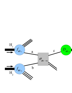
Figure 1: Schematic sketch for the amplitude of the leading factorized processes for production of a single hadron $H_{3}$ in the collision of two hadrons $H_{1}$ and $H_{2}$. The thin lines represent single partons connecting the soft (i.e. long distance) processes within the hadrons with the hard (i.e. short-distance) scattering. Soft and hard processes are depicted by round blobs and boxes respectively. The probability distributions referring to the soft and hard processes are defined as the parton distributions $f$ or fragmentation functions $D$, and the hard partonic cross section $\sigma_{a+b\to c}$ resp.

The factorization of the cross section can schematically be written as

$$d\sigma_{H_{1}+H_{2}\to H_{3}+X}=\sum_{a,b,c}f_{a/H_{1}}\otimes f_{b/H_{2}}\otimes d\sigma_{a+b\to c+x}\otimes D_{c/H_{3}}+\mathrm{power\>suppr.\>terms}$$ (1)

where $\sigma_{a+b\to c+x}$ is the hard partonic cross section involving a large momentum transfer. Processes involving other “associations”, most notably those with more partons taken from one hadron are of higher twist and suppressed by powers of $1/Q\sim 1/P_{T}$. The convolution signs mean that the parton momenta connecting blobs and hard cross sections have to be integrated, if not fixed by kinematics. This will become more clear when concrete examples are discussed further below.

A few additional remarks are in order.

• Here we will only deal with collinear factorization. This is sufficient for processes with a single hard scale $Q$, or even for processes with different scales $Q_{1}$, $Q_{2}$ (then resummations are needed) as long as all scales are large. So called $k_{T}$-factorization is needed for processes with one hard and one soft scale and will not be discussed here [17, 18]. Practically this means partons can kinematically always be treated as collinear with their parent hadrons, which simplifies the momentum integrals in the factorization formulas tremendously.

• At first we will only discuss leading twist processes. With scales of the order of a few GeV this is sufficient for single hadrons. However, in the case of nuclei we will see that some higher twist processes are enhanced and become important.

• We will also refrain from discussing particle production in the limit of very large center of mass energy, when the gluon distribution of hadrons saturates. For large nuclei this limit might be reached at RHIC energies and particle production from this Color Glass state could be dominant for particles at lower $P_{T}$ (from scattering of partons with low Bjorken-$\xi$ in the initial wave function). With the saturation scale $Q_{s}$ for gold nuclei at RHIC energies estimated to be smaller than 2 GeV [19], the high-$P_{T}$ domain should be safely in the region of collinear factorization. We will revisit this topic in the section about initial conditions for hydrodynamics. For the most recent reviews of the Color Glass Condensate see e.g. [20, 21].

• Collinear factorization has been rigorously proven in very few cases, and even for simple processes there are examples where factorization breaks at a certain order in $1/Q^{n}$ [22]. This is particularly worrisome for collisions of nuclei where multiple scattering and higher twist corrections are enhanced. We will always assume factorization of initial states and hard processes here. On the other hand the study of final state effects in nuclear collisions is by definition an investigation of how factorization and universality are broken for long-distance final states.

2.1.1 Cross Sections of Partons

The factorization theorems mentioned above make sure that the underlying hard parton cross sections are infrared-safe. They can be calculated in a perturbative expansion. Singularities from radiative corrections can be factored off into the long-distance part that is described by parton distributions and fragmentation functions. E.g., for our example of single hadron production at large momentum the underlying parton cross section can be written as

$$d\sigma_{a+b\to c+x}=\alpha_{S}^{2}d\sigma_{a+b\to c+x}^{\mathrm{(LO)}}+\alpha_{S}^{3}d\sigma_{a+b\to c+x}^{\mathrm{(NLO)}}+\ldots.$$ (2)

Leading order (parton model) cross sections are easily calculated. For further processing parton cross sections $a+b\to c+d$ are most easily parameterized in terms of the Lorentz-invariant Mandelstam variables $s=(p_{a}+p_{b})^{2}$, $t=(p_{a}-p_{c})^{2}$, $u=(p_{a}-p_{d})^{2}$ where $p_{a}$, $p_{b}$, etc. are the four-momenta of partons $a$, $b$, etc. For example for the scattering of two different quark (or antiquark) species $q$ and $q^{\prime}$

$$\frac{d\sigma^{\mathrm{(LO)}}_{q+q^{\prime}\to q+q^{\prime}}}{dt}=\frac{\pi\alpha_{s}^{2}}{s^{2}}\frac{N_{c}^{2}-1}{2N_{c}^{2}}\frac{s^{2}+u^{2}}{t^{2}}$$ (3)

where $N_{c}=3$ is the number of colors, and by definition we have averaged over ingoing spins and colors and summed over outgoing spins and colors (we have kept the coupling constant as part of the cross section unlike indicated in (2)). A comprehensive table for production of light partons and photons can be found in the review article by Owens [23].

Next-to-leading (NLO) calculations of parton production is much more challenging. The basic matrix elements can be found in the work by Ellis and Sexton [24]. The one- and two-jet cross sections were e.g. worked out in [25, 26]. Several numerical codes are available for jet, hadron or photon production at NLO accuracy, performing the required phase space integrals and cancellation of singularities. An excellent starting point for the interested reader is the PHOX collection by Aurenche and collaborators [27].

We have to discuss an important point here. From the NLO-level on cross sections with parton final states are no longer well defined, i.e. infrared-safe. In fact we can only define cross sections either into hadrons or jets, i.e. sprays of hadrons defined by energy in a restricted region of phase space. At leading order one can make the convenient identification jet = parton. At NLO two partons can be so close together in phase space that they have to be replaced with one jet.

In nuclear collisions with its emphasis on final state effects the convenient identification becomes a necessary simplification that allows for the treatment of energy loss and other effects on the basis of single partons. This is also one reason why a large fraction of literature on heavy ion collisions uses leading order calculations. Recently, more and more NLO-based calculations have been presented. In that case caution is in order if they are combined with final state effects based on a single parton picture.

The basis for the use of LO cross sections is the fact that for single and double hadron and photon $P_{T}$-spectra LO accuracy yields reasonably good results. It turns out that for collisions of single hadrons

$$\frac{d\sigma^{\mathrm{(NLO)}}}{d^{2}P_{T}}=K\frac{d\sigma^{\mathrm{(LO)}}}{d^{2}P_{T}}$$ (4)

with a $K$-factor that is close to one and only weakly dependent on the momentum $P_{T}$ of the produced hadron [28]. For convenience $K$ is hence often approximated by a constant.

2.1.2 Parton Distributions and Fragmentation Functions

In the schematic factorization formula (1) $f_{a/H_{1}}$ and $f_{b/H_{2}}$ are parton distribution functions (PDFs) which describe the probabilities that partons $a$, $b$ can be found in hadrons $H_{1}$, $H_{2}$, resp., with given momenta. Note that factorization at leading twist provides a very satisfying probabilistic picture (there is no interference between amplitude and complex conjugated amplitude of the parton line connecting the hard cross section with bound states). Parton distributions are well-defined and gauge invariant matrix elements in QCD. They are also universal, i.e. their definition is independent of the particular process in which they occur.

Suppose hadron $H$ is moving with large momentum $P$ along the positive $z$ axis such that $P^{+}\to\infty$. We introduce the light cone components of a four-vector $p^{\mu}$ as $p^{\pm}=(p^{0}\pm p^{3})/\sqrt{2}$. The parton distribution for quarks and gluons in a light cone gauge ($A^{+}=0$) are defined as

$$f_{q/H}(\xi,\mu) =\int\frac{dy^{-}}{4\pi}e^{-i\xi P^{+}y^{-}}\left\langle H(P)\right|\bar{q}(y^{-})\gamma^{+}q(0)\left|H(P)\right\rangle$$ (5)

$$f_{g/H}(\xi,\mu) =\frac{1}{\xi P^{+}}\int\frac{dy^{-}}{2\pi}e^{-i\xi P^{+}y^{-}}\left\langle H(P)\right|F_{a}^{+\nu}(y^{-})F_{a\,\nu}^{\>\>\>\>+}(0)\left|H(P)\right\rangle$$ (6)

Here $\left|H(P)\right\rangle$ is the suitably normalized single hadron state, (note that an averaging over hadron spins is usually silently implied in the notation $\left\langle H(P)\right|\ldots\left|H(P)\right\rangle$), and $q$ and $F$ are the operators for quark and gluon fields. $\xi$ with $0<\xi<1$ is the momentum fraction of the parton in the parent hadron. In light cone gauge it is straight forward to interpret these matrix elements as quark and gluon counting operators. Note again that these matrix elements can not be evaluated perturbatively for hadrons or nuclei. The left panel of Fig. 2 shows a diagrammatic representation of a parton distribution function in light cone gauge.

Radiative corrections introduce a weak, logarithmic scale dependence. The first radiative corrections are shown in the right panel of Fig.  2 for a light cone gauge. Resummation of these diagrams lead to the DGLAP evolution equations which determine the running of parton distributions $f_{a/H}(\xi,\mu)$ with the scale $\mu$ [29, 30, 31]. For a parton $a$ they are

$$\frac{\partial f_{a}(\xi,\mu)}{\partial\ln\mu}=\frac{\alpha_{s}}{\pi}\int_{x}^{1}\frac{dy}{y}\sum_{b}P_{b\to a}(y)f_{b}\left(\frac{\xi}{y},\mu\right)$$ (7)

where the set of $P_{b\to a}(y)$ are called the splitting functions. This notion is easily explained with a look at the right panel of Fig. 2 whose diagrams represent the $q\to q$ splitting function which is

$$P_{q\to q}(y)=C_{F}\left(\frac{1+y^{2}}{1-y}\right)_{+}+C_{F}\frac{3}{2}\delta(y-1)$$ (8)

where $C_{F}=4/3$ is the color factor. Virtual corrections make a contribution at $y=1$ which introduces the $\delta$-function term and regularizes the singularity in the first term via the $+$ description: $(f(y)/[1-y])_{+}\to[f(y)-f(1)]/[1-y]$ for the integral over any function $f(y)/[1-y]$. More details and the full set of splitting functions are discussed in [10].

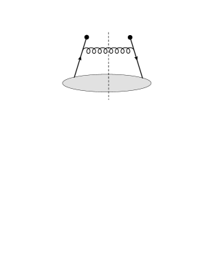
Figure 2: Left panel: diagrammatic representation of a quark parton distribution. The two “end” points represent the positions of the quark fields in Eq. (5). Right panel: diagrams with lowest order radiative corrections for the quark parton distribution in light cone gauge. Note that there are generally more diagrams in different gauges due to the presence of a gauge link.

While the $\mu$-dependence is hence perturbatively calculable, the $\xi$-dependence can only be extracted from fits to data. This relies heavily on data from the “clean” deep-inelastic scattering (DIS) process. Very accurate parameterizations including estimates of uncertainties are available for protons and, via isospin symmetry, for neutrons in a wide range of about $10^{-5}<x<0.5$. The most used parameterizations are from the CTEQ [32, 33] and MRST collaborations [34, 35]. The Durham data base has comprehensive information about PDFs [36]. Parton distributions of nuclei are discussed further below.

Fragmentation functions $D_{c/H}(z,\mu)$ give the reverse probability that hadron $H$ hadronizes from parton $c$ in the vacuum with a certain momentum fraction $z$ of the parent parton [37]. Unlike the case of parton distributions a complete sum over states can not be removed and hence fragmentation functions can not be written as a single forward matrix element. Instead we have

$$D_{q/H}(z,\mu)=z\int\frac{dy^{-}}{4\pi}e^{-iP^{+}y^{-}/z}\left\langle H(P)\right|\bar{q}(y^{-})\left|0\right\rangle\gamma^{+}\left\langle 0\right|q(0)\left|H(P)\right\rangle$$ (9)

for a quark $q$ with large light cone momentum $P^{+}$. As for parton distributions, vacuum fragmentation functions have been parameterized, mostly from hadron production data in $e^{+}+e^{-}$ collisions, but uncertainties in the fits are appreciable, even for quite common hadrons like protons and kaons. In addition, some sets are not isospin-separated, i.e. they only parameterize processes like $u+\bar{u}\to\pi^{+}+\pi^{-}$. This uncertainty in the theoretical baseline makes the search for nuclear effects more challenging. The most widely used parameterizations in heavy ion physics are the sets by Kniehl et al. (KKP) [38] and Albino et al. (AKK) [39], Hirai et al. (HKNS) [40] and deFlorian et al. (DSS) [41, 42]. The latter ones include iso-spin separation, partially also including data from $p+p$ collisions.

2.1.3 Factorized Cross Sections

In this subsection we will summarize some often used factorization formulas for hadron or jet production at leading order. They can be used together with the list of leading order parton cross sections in [23] and the parton distributions and fragmentation functions referenced above to make estimates for rates of hadron and jet production. Our starting point is the differential production cross section of two partons $c$ and $d$ from two hadrons $A$ and $B$

$$d\sigma_{AB\to cd}=\sum_{a,b}f_{a/A}(\xi_{a})f_{b/B}(\xi_{b})d\sigma_{ab\to cd}\,.$$ (10)

We need to introduce some notation for the kinematics. Let the momenta of the parent hadrons be $P_{A}$ and $P_{B}$ in positive and negative direction, resp., along the $z$-axis in the center of mass frame of the hadrons. We assume that $P\equiv P_{A}^{+}=P_{B}^{-}$ is larger than any relevant masses. Note that the kinematics in (10) is fixed at leading order with $\xi_{a}=p_{a}^{+}/P$ and $\xi_{b}=p_{b}^{-}/P$, resp. where $p_{a}$, $p_{b}$, $p_{c}$ and $p_{d}$ are the momenta of the four partons.

One can easily deduce the cross section for a di-jet event with final rapidities $y_{c}$ and $y_{d}$ and transverse momentum $p_{T}$ (the transverse momenta of $c$ and $d$ are equal and opposite),

$$\frac{d\sigma_{AB\to cd}}{2\pi p_{T}dp_{T}dy_{c}dy_{d}}=\sum_{a,b}\xi_{a}f_{a/A}(\xi_{a})\xi_{b}f_{b/B}(\xi_{b})\frac{1}{\pi}\frac{d\sigma_{ab\to cd}}{dt}$$ (11)

where the momentum fractions are fixed to be

$$\xi_{a}=\frac{2p_{T}}{s}\left(e^{y_{c}}+e^{y_{d}}\right)\,,\qquad\xi_{b}=\frac{2p_{T}}{s}\left(e^{-y_{c}}+e^{-y_{d}}\right)\,.$$ (12)

Note that all Mandelstam variables $s$, $t$, $u$ are defined on the level of partons $a,b,c,d$. In particular

$$t=-\xi_{a}p_{T}\sqrt{S}e^{-y_{c}}$$ (13)

where $S=(P_{A}+P_{B})^{2}=2P^{2}$ is the total center of mass energy squared of the two hadrons.

For single jet events we have to integrate one of the final parton momenta. This introduces effectively one non-trivial integral which is usually rewritten as an integral over one of the initial parton momentum fractions. For a jet with transverse momentum $p_{T}$ and rapidity $y$ we find

$$\frac{d\sigma_{AB\to c+X}}{2\pi p_{T}dp_{T}dy}=\sum_{a,b,d}\int_{\xi_{\mathrm{min}}}^{1}d\xi_{a}f_{a/A}(\xi_{a})f_{b/B}(\xi_{b})\frac{2}{\pi}\frac{\xi_{a}\xi_{b}}{2\xi_{a}-\xi_{T}e^{y}}\frac{d\sigma_{ab\to cd}}{dt}$$ (14)

where $\xi_{b}$ is fixed to

$$\xi_{b}=\frac{\xi_{a}\xi_{T}e^{-y}}{2\xi_{a}-\xi_{T}e^{y}}\,,$$ (15)

and the integration boundary (to keep $\xi_{b}<1$ for fixed $y$, $p_{T}$) is

$$\xi_{\mathrm{min}}=\frac{\xi_{T}e^{y}}{2-\xi_{T}e^{-y}}.$$ (16)

We have introduced the useful scaling variable $\xi_{T}=2p_{T}/\sqrt{S}$.

In order to arrive at cross sections for hadrons we have to multiply the differential cross section for partons with the corresponding fragmentation functions. The resulting phase space integrals are often shifted to be integrals over the initial parton momentum fractions $\xi_{a}$ and $\xi_{b}$. For applications in heavy ion physics we rather adopt a different way that keeps factorizability between the fragmentation functions on one hand and the parton cross section plus parton distributions on the other hand explicit. For two hadrons $C$ and $D$ with momenta $P_{TC}$ and $P_{TC}$ we can write

$$\frac{dN_{CD}}{2\pi P_{TC}dP_{TC}P_{TD}dP_{TD}dy_{C}dy_{D}}=\sum_{c,d}\int_{z_{c,\mathrm{min}}}^{1}\frac{dz_{c}}{z_{c}^{2}}\int_{z_{d,\mathrm{min}}}^{1}\frac{dz_{d}}{z_{d}^{2}}\\ \times\frac{dN_{cd}}{2\pi p_{Tc}dp_{Tc}p_{Td}dp_{Td}dy_{C}dy_{D}}D_{c/C}(z_{c})D_{d/D}(z_{d})\,.$$ (17)

This is a very general formula that connects a distribution function of partons $c$, $d$ with momenta $p_{c}=P_{C}/z_{c}$, $p_{d}=P_{D}/z_{d}$, resp. in the final state to hadrons $C$, $D$. Of course the applicability of this formula still requires the collinear fragmentation picture to hold in this much generalized setting. Nevertheless, derivatives from Eq. (17) are often used to model final state interactions for hadron production in nuclear collisions. There might be kinematic constraints that lead to lower bounds on the integrals over $z_{c}$ and $z_{d}$ whose exact specification will depend on the distribution $N_{cd}$ of partons.

For completeness and further clarification let us discuss the more familiar special case of hadron production in a regime where final state interactions can be neglected, e.g. in $p+p$ collisions. The formula above holds also for cross sections, $N_{CD}\to\sigma_{AB\to CD}$, and the partonic cross section is given by (11) times an obvious phase space factor $1/p_{Td}\,\delta(p_{Tc}-p_{Td})$. This factor can be used to cancel the integral over $z_{d}$ to lead to

$$\frac{d\sigma_{AB\to CD}}{2\pi P_{TC}dP_{TC}P_{TD}dP_{TD}dy_{C}dy_{D}}\\ =\frac{1}{P_{TC}P_{TD}}\sum_{a,b,c,d}\int_{z_{\mathrm{min}}}^{z_{\mathrm{max}}}\frac{dz_{c}}{z_{c}}\xi_{a}f_{a/A}(\xi_{a})\xi_{b}f_{b/B}(\xi_{b})\frac{1}{\pi}D_{c/C}(z_{c})D_{d/D}(z_{d})\frac{d\sigma_{ab\to cd}}{dt}$$ (18)

where

$$z_{d}=z_{c}\frac{P_{TD}}{P_{TC}}\,,\qquad z_{\mathrm{max}}=\mathrm{min}\left\{1,\frac{P_{TC}}{P_{TD}}\right\}\,,\qquad z_{\mathrm{min}}=\frac{2P_{TC}}{\sqrt{S}}\mathrm{max}\left\{\cosh y_{C},\cosh y_{D}\right\}\,.$$ (19)

Note that $\xi_{a}$ and $\xi_{b}$ are given by (12) with $p_{Tc}=P_{TC}/z_{c}$ and $p_{Td}=P_{TD}/z_{d}$.

For single hadron production we can provide a similar general formula for fragmentation from a distribution of partons $N_{c}$,

$$\frac{dN_{C}}{2\pi P_{T}dP_{T}dy}=\sum_{c}\int_{z_{\mathrm{min}}}^{1}\frac{dz}{z^{2}}D_{c/C}(z)\frac{dN_{c}}{2\pi p_{T}dp_{T}dy}\,.$$ (20)

It can be applied if collinear fragmentation is the correct description of hadronization of an ensemble of partons and obviously $p=P/z$. The special case of single hadron production in collisions with negligible final state interactions gives the formula

$$\frac{d\sigma_{AB\to C+X}}{2\pi P_{T}dP_{T}dy}=\sum_{a,b,c,d}\int_{z_{\mathrm{min}}}^{1}\frac{dz}{z^{2}}D_{c/C}(z)\int_{\xi_{\mathrm{min}}}^{1}d\xi_{a}f_{a/A}(\xi_{a})f_{b/B}(\xi_{b})\frac{2}{\pi}\frac{\xi_{a}\xi_{b}}{2\xi_{a}-\xi_{T}e^{y}}\frac{d\sigma_{ab\to cd}}{dt}$$ (21)

where

$$z_{\mathrm{min}}=\frac{2P_{T}}{\sqrt{S}}\cosh y\,,$$ (22)

and the other kinematic variables can be inferred from (15) and (16).

For an alternative way of handling the phase space integrals in terms of hadron production see [23]. Let us point out once more that the convenient identification of single partons and jets is only valid in the context of leading order calculations.

2.1.4 Photons

In principle, photons with high transverse momentum $P_{T}$ can be treated in a fashion very similar to hadrons or jets. We usually do not consider photons from decays of hadrons (predominantly $\pi^{0}$) long after the collision. After subtracting those decay photons we are left with the “direct” photons produced in the collision. Photon yields produced directly in the hard process can be calculated via Eq. (14) together with the corresponding parton level processes. At leading order, the cross sections of the annihilation and Compton diagrams, $q+\bar{q}\to\gamma+g$ and $g+q\to\gamma+q$, resp. can be found in the work by Owens [23].

Another way to produce direct photons is as bremsstrahlung in hard process like $g+g\to q+\bar{q}$. One of the outgoing quarks can radiate a collinear photon while fragmenting. This process can be described by photon fragmentation functions [23, 43]. Eq. (20) together with the usual set of hard parton processes and photon fragmentation functions are used to compute this contribution. At next-to-leading order, bremsstrahlung and hard photon radiation in the final state have to be calculated in a consistent scheme to separate large angle and collinear photon radiation [44, 45]. NLO direct photon calculations have had some difficulties in the past to describe all aspects of photon production in hadronic collisions [46]. The theoretical understanding has been improved in recent years by the use of various resummation techniques [47, 48]. The PHOX codes can also be used for NLO calculations of direct photon production.

Photon-hadron and photon-jet pair production is a particularly hot topic in heavy ion collisions as we will discuss in more detail later. Their yields with both initial hard and bremsstrahlung photons can also be calculated in a straight forward way from the factorization formulas in the last subsection. Fragmented photons can in principle be distinguished from prompt hard photons since the latter are not accompanied by hadrons close by in phase space while the former are usually part of a jet cone. Experimentally, isolation cuts for photons can help to suppress the bremsstrahlung contribution and give access to more detailed information.

In nuclear collisions there are additional sources of direct photons. We will discuss jet conversion into photons in the subsection about final state interactions. There is also thermal radiation from the hot hadronic matter, and, if energy densities are large enough, from the partonic QGP phase. In fact the latter is one of the key observables that we would like to study at RHIC, since the thermal photon spectrum can work as a direct (though time- and space-averaged) thermometer of the quark gluon plasma. To compute the photon spectrum the time-evolution of the QGP fireball has to be folded with rates as a function of the local temperature and chemical potential. The time evolution is naturally done through a hydrodynamic model as discussed in Sec. 3 of this review. The rates can be calculated perturbatively if the temperature $T$ is large enough to render the strong coupling constant small, $g\ll 1$. Although there is some doubt whether the maximum temperatures at RHIC ($T<450$ MeV) are sufficient to warrant a perturbative description the perturbative computation of thermal photon rates has been a sustained effort over many years [49, 50, 51]. The complete leading order results have been given by Arnold, Moore and Yaffe in [52, 53]. Additional photon radiation could be emitted in the pre-equilibrium phase. In particular, the fact that quarks and gluons are not in chemical equilibrium early on could affect photon rates and would not be mimicked well by hydro codes initialized at very early times. Estimates for pre-equilibrium photon yields in a transport approach can be found in [54].

2.2 Nuclear Collisions: Initial State Effects

Perturbative techniques and factorization have first been developed for scattering involving individual hadrons. The basic principles should be valid if one or both of the scattering partners are bound in a nucleus. In fact, the small binding energies and slow relative motion of nucleons should not have large impact on scattering at large momentum transfer. However, the larger volumes filled with nuclear matter surrounding the point-like hard interaction should potentially lead to rescattering both in the initial and final state. In this subsection we will discuss the most relevant nuclear effects in the initial state.

2.2.1 Shadowing and Nuclear Parton Distributions

Individual nucleons are clearly distinguishable building blocks of nuclei. Hence we expect parton distributions in a nucleus with $Z$ protons and $A-Z$ neutrons to be well represented by a linear superposition of parton distributions of the individual protons $p$ and neutrons $n$,

$$f_{a/A}(\xi,\mu)=\left(\frac{Z}{A}f_{a/p}(\xi,\mu)+\frac{A-Z}{A}f_{a/n}(\xi,\mu)\right)R_{A}(\xi,\mu)$$ (23)

The remaining non-trivial nuclear modification $R_{A}$ was expected to be small until it was found by the EMC collaboration that deep-inelastic scattering off nuclei leads to sizable differences between free and bound nucleons [55]. Note that nuclear parton distributions are usually normalized to one nucleon.

Despite considerably larger uncertainties compared to free nucleon parton distributions we can now identify four distinct regions of behavior in the momentum fraction $\xi$ which are indicted in Fig. 3, see [56, 57, 58] and references therein.

• Fermi motion enhancement, $\xi>0.8$: when the parton carries most of the momentum of the nucleon the Fermi motion of the nucleon itself in the nucleus becomes important.

• EMC effect (proper), $0.3<\xi<0.8$: the kinematic region of the original discovery, named after the experiment, exhibits a suppression $R_{A}(\xi)<1$ which is usually explained with nuclear binding effects.

• Antishadowing, $0.1<\xi<0.3$: a region of enhancement of nuclear parton distributions required by momentum sum rules.

• Shadowing, $\xi<0.1$: a region of possibly large suppression of parton distributions. It can be understood through multiple scattering in the nuclear rest frame, or parton fusion in an infinite momentum frame. In the deep shadowing (small-$\xi$) region this might lead to a color glass condensate picture. We refer to [58] for a modern review of models for the shadowing effect.

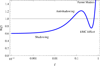
Figure 3: Schematic sketch of the expected behavior of the ratio $R_{A}$ of nuclear parton distributions compared with free nucleon parton distributions. The distinct regions, the Fermi motion region, the EMC region and the shadowing and antishadowing regions are visible. The ratio $R_{A}$ is directly reflected in the ratio of single particle spectra in $p+$A collisions to $p+p$ collisions as a function of $P_{T}$.

A parton with 10 GeV/$c$ transverse momentum produced at midrapidities ($y=0$) in collisions at RHIC energies ($\sqrt{s_{NN}}=200$ GeV) comes from initial parton momentum fractions around $\xi_{T}=2p_{T}/\sqrt{S_{NN}}=0.1$. Hence it is easy to see that for perturbative calculations at RHIC mostly the shadowing and anti-shadowing regions are of importance. For not too small momentum fractions $\xi$ nuclear parton distributions are still in the universal DGLAP regime. They can be measured in deep inelastic scattering on nuclei, while the perturbative evolution in the scale $\mu$ can be used as a consistency check. The parameterizations (which are often parameterizations of the modification $R_{A}$ for specific sets of free nucleon parton distributions) can then be used for hadron-nucleus and nucleus-nucleus collisions. DGLAP parameterizations are available from several groups [59, 60, 61, 62, 63, 64, 65, 66]. Some, like the EPS08 and EPS09 parameterizations [61, 62], already include some RHIC data in the DGLAP fit. This has been done to improve the lack of suitable deep-inelastic scattering data on nuclei. Previous deep-inelastic scattering experiments off nuclei cover only large $\xi$ and have very little power to constrain the nuclear gluon distribution. This situation leaves us with huge theoretical uncertainties on the nuclear gluon distribution below $\xi\approx 0.05$. Fig. 4 shows several fits for modification factors for valence quarks, sea quarks and gluons respectively. The spread of possible values for the nuclear gluon distribution is truly remarkable. This uncertainty has profound consequences for pQCD predictions at LHC energies where the average parton $\xi$ will be much smaller than at RHIC.

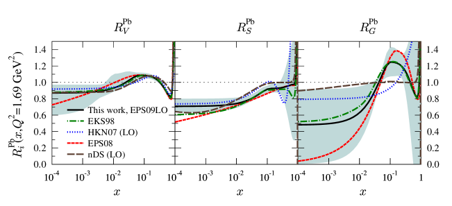
Figure 4: Comparison of different leading order DGLAP parameterizations of the nuclear modification $R_{\mathrm{Pb}}(x,\mu)$ for lead nuclei at $\mu=1.3$ GeV. The parameterization correspond to EKS98 [59], EPS08 [61], EPS09 [62], HKN07 [65], and nDS [66]. The large theoretical uncertainties at low momentum fraction $x$, in particular for the gluons, is clearly demonstrated. Figure reprinted from [62] with permission from JHEP.

2.2.2 Higher Twist Corrections

Nuclear corrections to the parton distributions deal with the effects of nuclear binding on the long-distance behavior of a process. One can also ask the question whether the hard process between partons is affected as well. Indeed it turns out that certain high-twist corrections become important in collisions involving nuclei. Corrections beyond leading twist were first characterized in terms of new operators beyond parton distributions that appear in the operator production expansion. Twist $t$ was defined as the dimension minus the spin of a local operator. The definition can be generalized to apply also to situations where an operator product expansion is not available. The leading twist operators in parton distributions, $\bar{q}\gamma^{+}q$ and $F^{+\mu}F_{\mu}^{\,\,+}$, are classified as twist $t=2$. We will use higher twist as a simple power counting scheme in terms of the large scale $Q$, such that a twist-$t$ contribution is suppressed by $1/Q^{t-2}$ compared to leading twist. Jaffe’s review [67] offers a discussion of both the rigorous and the power counting definition of twist.

Higher twist effects are obviously important if the large scales $Q$ becomes to small (close to non-perturbative scales), or if other enhancement effects weaken the power suppression. It was first pointed out by Luo, Qiu and Sterman [68, 69, 70] that in large nuclei with mass number $A$ some operators do not follow a classification in terms of an expansion in $\Lambda/Q\ll 1$, but rather in the parameter

$$\Lambda A^{1/3}/Q\sim\Lambda^{2}L/Q>>\Lambda/Q\,.$$ (24)

Here $\Lambda$ is a soft scale (of the order or $\Lambda_{\mathrm{QCD}}$ or the constituent quark mass) and $L\sim A^{1/3}/\Lambda$ is the thickness of the nucleus. $L$ comes into play because in thick nuclear matter multiple hard scattering is possible and its probability increases with thickness. Multiple scattering should not modify the total cross section very much, but we expect some observables, e.g. transverse momentum spectra, to be significantly altered by multiple additional “kicks” that a scattered particle experiences. The Cronin effect discussed below is a good example.

We want to review a simple example, the nuclear Drell-Yan process $A+A\to l^{+}+l^{-}+X$ [71, 72, 73, 74]. At leading order $\mathcal{O}(\alpha_{s}^{0})$, and leading twist the virtual photon is produced through a simple quark-antiquark annihilation, $q+\bar{q}\to l^{+}+l^{-}$, see left panel in Fig. 5. The corresponding cross section for dilepton pairs of mass $Q$ and (pair) transverse momentum $q_{T}$ is

$$\frac{d\sigma_{AB\to l^{+}+l^{-}}}{dQ^{2}dq_{T}^{2}}=\sigma_{\mathbf{DY}}\delta(q_{T}^{2})\sum_{q}e_{q}^{2}\int_{B_{a}}^{1}\left[f_{q/A}(\xi_{a})f_{\bar{q}/B}(\xi_{b})+f_{\bar{q}/A}(\xi_{a})f_{q/B}(\xi_{b})\right]d\xi_{b}$$ (25)

where

$$\sigma_{\mathbf{DY}}=\frac{4\pi}{3N_{c}}\frac{\alpha_{em}^{2}}{SQ^{2}}$$ (26)

essentially is the cross section between partons $q$ and $\bar{q}$, $N_{c}=3$, $e_{q}$ is the charge of quark $q$ in units of $e$, and $\xi_{a}=Q^{2}/(\xi_{b}S)$ is fixed with $B_{a}=Q^{2}/S$. (25) is a straight forward but nevertheless questionable result. The $q_{\perp}$-spectrum is actually not well defined in the collinear limit. Indeed the presence of two scales $q_{T}<<Q$ presents additional problems. The safe way to discuss this result is by using moments in $q_{\perp}$-space. The lowest moment is the cross section differential with respect to the mass squared

$$\frac{d\sigma_{AB\to l^{+}l^{-}}}{dQ^{2}}=\int_{0}^{\infty}\frac{d\sigma_{AB\to l^{+}l^{-}}}{dQ^{2}dq_{\perp}^{2}}dq_{T}^{2}\,,$$ (27)

while the next moment can be used to define the average transverse momentum squared

$$\left\langle q_{T}^{2}\right\rangle=\frac{\int_{0}^{\infty}\frac{d\sigma_{AB\to l^{+}l^{-}}}{dQ^{2}dq_{T}^{2}}q_{T}^{2}dq_{T}^{2}}{\frac{d\sigma_{AB\to l^{+}l^{-}}}{dQ^{2}}}.$$ (28)

At leading order and leading twist $\langle q_{\perp}^{2}\rangle=0$ which is also true for all higher moments.

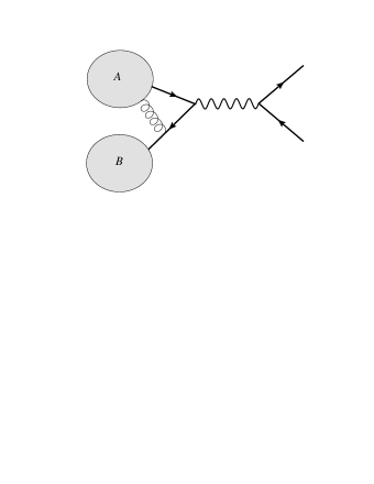
Figure 5: Left panel: Drell-Yan at leading twist and leading order in $\alpha_{s}$: quark-antiquark annihilation. Right panel: A nuclear enhanced twist-4 correction in $A+A$ collisions that corresponds to double scattering of the quark from the proton in the nucleus. First the quark scatters off a soft gluon and then annihilates with an antiquark.

The first nuclear enhanced higher twist correction corresponds to double scattering of one of the quarks off an additional gluon from the other nucleus, e.g. $q+\bar{q}g\to l^{+}+l^{-}$, see right panel in Fig. 5. The cross section is

$$\frac{d\sigma_{AB\to l^{+}+l^{-}}^{(2)}}{dQ^{2}dq_{T}^{2}}=-\delta^{\prime}(q_{T}^{2})\sigma_{\mathbf{DY}}\frac{4\pi\alpha_{s}}{N_{c}}\sum_{q}e_{q}^{2}\\ \times\int_{B_{a}}^{1}\left[f_{q/A}(\xi_{a})T_{\bar{q}g/B}(\xi_{b})+f_{\bar{q}/A}(\xi_{a})T_{qg/B}(\xi_{b})+T_{qg/A}(\xi_{a})f_{\bar{q}/B}(\xi_{b})+T_{\bar{q}g/A}(\xi_{a})f_{q/B}(\xi_{b})\right]d\xi_{b}$$ (29)

Note that there is a derivative on the $\delta$-function. The new matrix elements $T_{ab/A}$ measure a “soft-hard” two-parton density in the nucleus, e.g.

$$T_{qg/A}(\xi)=\int dy_{4}^{-}\frac{dy_{3}^{-}}{2\pi}\frac{dy_{1}^{-}}{2\pi}e^{i\xi P^{+}y_{1}^{-}}\Theta(y_{1}^{-}-y_{3}^{-})\Theta(-y_{4}^{-})\left\langle A(P)\right|\bar{q}(0)\gamma^{+}q(y_{1}^{-})\\ \times F_{a}^{+\nu}(y_{3}^{-})F_{a\,\nu}^{\>\>\>\>+}(y_{4}^{-})\left|A(P)\right\rangle$$ (30)

where $P^{+}$ is the large momentum component of a nucleon. Soft-hard in this particular case means that the quark or antiquark has a finite momentum fraction $\xi$ while the gluon is very soft. Formally the soft-hard matrix elements are limits of more general 2-parton distributions $f^{(2)}_{qg/A}(\xi_{q},\xi_{g})$ with

$$T_{qg/A}(\xi_{q})=\lim_{\xi_{g}\to 0}\xi_{g}f^{(2)}_{qg/A}(\xi_{q},\xi_{g})\,.$$ (31)

Luo, Qiu and Sterman have classified the relevant twist-4 matrix elements that show nuclear enhancement. They all have a probabilistic interpretation as 2-parton densities and they lead to soft-hard and hard-hard double scattering on the parton level. The actual nuclear enhancement factor comes from unrestricted spatial integrations along the light cone. The coordinates associated with the two partons — corresponding to $y_{1}^{-}/2$ and $(y_{3}^{-}+y_{4}^{-})/2$ in Eq. (30) — can be as far apart as the nuclear matter extends along the light cone. Parametrically we have

$$T_{qg/A}(\xi)\sim A^{1/3}\Lambda^{2}$$ (32)

where $\Lambda$ is a soft scale and $A$ denotes the mass number of nucleus $A$.

To arrive at infrared-safe results we again take moments. We note that $t=4$ double scattering does not make a contribution to the integrated mass spectrum, $d\sigma^{(2))}/dQ^{2}=0$, or the total cross section. However, it leads to non-vanishing transverse momentum, despite the use of collinear factorization and the absence of radiation,

$$\langle q_{T}^{2}\rangle=\frac{4\pi\alpha_{s}}{N_{c}}\frac{\sum_{q}e_{q}^{2}\int_{B_{a}}^{1}\left[f_{q/A}(\xi_{q})T_{\bar{q}g/B}(\xi_{b})+f_{\bar{q}/A}(\xi_{a})T_{qg/B}(\xi_{b})+T_{qg/A}(\xi_{a})f_{\bar{q}/B}(\xi_{b})+T_{\bar{q}g/A}(\xi_{a})f_{q/B}(\xi_{b})\right]d\xi_{b}}{\sum_{q}e_{q}^{2}\int_{B_{a}}^{1}\left[f_{q/A}(\xi_{a})f_{\bar{q}/B}(\xi_{b})+f_{\bar{q}/A}(\xi_{a})f_{q/B}(\xi_{b})\right]d\xi_{b}}\,.$$ (33)

The $t=4$ matrix elements are universal functions that could in principle be measured, but useful information is scarce. Most of the time the soft-hard matrix elements are simply modeled using the shape of the hard parton distribution

$$T_{qg/A}(\xi)=\lambda^{2}A^{1/3}f_{q/A}(\xi)$$ (34)

where $\lambda$ is a parameter with the dimension of energy which parameterizes the strength of the soft gluon field. For a symmetric situation with both nuclei being identical this leads to the simple estimate

$$\langle q_{T}^{2}\rangle\approx\frac{4\pi\alpha_{s}}{N_{c}}2\lambda^{2}$$ (35)

Higher twist corrections for $t>4$, correspond to multiple scattering beyond double scattering. It is possible to identify the operators with maximum nuclear enhancement $\sim A^{(t-2)/6}$ and they can be resummed in certain situations. This is safe to do for Drell-Yan in $p+$A collisions where the proton can be treated at leading twist [74, 75]. The resulting effect is a diffusion of $q_{T}$ in transverse momentum space. However, generally caution is necessary in nuclear collisions. Although the Drell-Yan process is rather simple, with no non-perturbative hadronic structure measured in the final state, factorization still breaks down beyond twist $t=4$ [22]. In other words, while nuclear enhanced higher twist corrections can be reliably calculated for Drell-Yan in $p+A$, there are true non-perturbative contributions that invalidate this expansion in $A+A$ collisions at the level of twist-6.

Nuclear enhanced higher twist corrections have been considered for several observables, including deep-inelastic scattering on nuclei [76], jets and dijets in electron-nucleus collisions [70, 77], Drell-Yan both at low and high $q_{T}$ [71, 74, 75], direct photon production [78], and photon bremsstrahlung for jets [79]. Note that higher twist corrections can appear both as initial and final state interactions. In fact, in most cases higher twist corrections could lead to both effects and can not be put in one of those two categories. However, those more general cases have not been considered in full detail, and we will mostly assume here that higher twist corrections in the initial and final state are independent of each other. The most important applications to date for the scope of this article are the Cronin effect (in the initial state) which we will discuss next, and medium-modified fragmentation functions (in the final state) which will be reviewed in more detail in the next subsection. We conclude by noting that there is a patchwork of relevant and useful calculations on the topic of nuclear enhanced higher twist, but a lack of comprehensive and systematic studies.

2.2.3 Cronin Effect

The Cronin effect was one of the first nuclear modifications discovered in experimental data [80]. It was found that cross sections of hadrons scale with a power of the atomic number $A$ that is larger than 1 for intermediate transverse momenta $P_{T}\approx 1$ GeV/$c$. This effect was found to not affect the total cross sections very much, and to die out like a power law at larger $P_{T}$. This is reminiscent of higher twist corrections and indeed these results can be interpreted in the framework of higher twist. Intuitively, the Cronin effect comes from multiple scatterings of partons on their way to the hard collision. These random kicks endow the parton with additional transverse momentum. This leads to a depletion of partons with very small (initial) intrinsic transverse momentum and an accumulation of partons at intermediate transverse momentum. At even larger values of $P_{T}$ the additional momentum kicks do not play a role and the effect decreases in importance.

The Cronin effect in its purest form can be studied in the case of dilepton or photon production in $p+$A or A+A collisions. Then it is guaranteed that deviations from the cross sections found in $p+p$ are initial state effects. We can simply refer to the discussion from the last subsection where we have established that higher twist corrections to the Drell-Yan process that correspond to double scattering lead to an increase in the average transverse momentum squared $\langle q_{T}^{2}\rangle$ which is proportional to $A^{1/3}$, and that a resummation of multiple scatterings leads to a Gaussian distribution of $q_{T}$ even at leading order in $\alpha_{s}$.

One can argue that these effects also increase $\langle P_{T}^{2}\rangle$ in hadron production, although it is not always clear how to distinguish the effects of initial and final state interactions. It is then quite common to refer to less rigorous but phenomenologically successful descriptions of the Cronin effect, see e.g. [81] for a review. These models are usually built on the notion of an intrinsic transverse momentum of partons in hadrons or nuclei. The concept of intrinsic transverse momentum $k_{T}$ is not compatible with collinear factorization but has a long history as a phenomenological extension of the former. True schemes for $k_{T}$-factorization do exist, but only for a handful of select processes, and they are technically more complex. Nevertheless many features of the Cronin effect can be described by a model in which the average $k_{T}^{2}$ is enhanced in nuclei through

$$\langle k_{T}^{2}\rangle_{pA,AA}=\langle k_{T}^{2}\rangle_{pp}+\delta k_{T}^{2}$$ (36)

where $\delta k_{T}^{2}$ scales with the thickness of nucleus $A$. This is also known as $k_{T}$-smearing.

One possible implementation is through the use of $k_{T}$-dependent “parton distributions”

$$\tilde{f}_{a/A}(\xi,{k}_{T},\mu)=\frac{1}{\pi\langle k_{\perp}^{2}\rangle}e^{-k_{T}^{2}/\langle k_{T}^{2}\rangle}f_{a/A}(\xi,\mu)$$ (37)

in which $\langle k_{T}^{2}\rangle$ can be fitted to the system size, or calculated from an underlying microscopic model, like a Glauber [82] or dipole model [83]. Reference [81] contains a compilation of parameters suitable for both RHIC and LHC energies. As a side remark we note that both shadowing and the Cronin effect are also natural consequences of gluon saturation and the mechanisms discussed here should smoothly transition to their color glass counterparts for very large center of mass energies [84, 85].

2.2.4 Phenomenological Consequences of Initial State Effects

Initial state effects are considered background effects in heavy ion physics. They are sometimes called cold nuclear matter effects, although the two terms are not synonymous. In fact, there are clearly final state effects in cold nuclear matter as seen in hadron production in $e+A$ collision by the HERMES experiment [86] and successfully described in terms of higher twist corrections [87]. For hadron production and similar process in $A+A$ collisions a factorization between initial and final state effects for hadron production is not obvious. It is one of the big assumptions of the hard probes program in heavy ion physics that final state effects can be factorized off and modeled separately from hard processes and initial state effects.

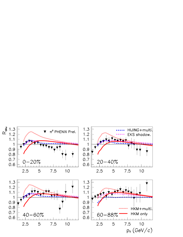
Figure 6: Cold nuclear matter effects for pion production in $d+$Au collisions at RHIC. The modification factor $R_{dAu}$ for $\pi^{0}$ is shown as a function of transverse momentum $P_{T}$. Data from the PHENIX experiment [89] is compared to several calculations using different sets of parton distributions with or without multiple scattering in the initial state. See text for details. Figure reprinted from [88] with permission from Elsevier.

One can analyze the effect of initial state interactions in nuclei by looking at hadron production in $p+$A and $d+$A collisions, and by studying photons and dileptons for $p+$A, $d+$A and A+A collisions. While these analyses are not yet complete, the picture that starts to emerge is that for Au ions at RHIC energies the initial state effects do not change the yield of hadrons for high $P_{T}>2$ GeV/$c$ by more than 20%.

Fig. 6 shows calculations by Levai et al. [88] of the nuclear modification factor

$$R_{dA}=\frac{dN^{dA}/dP_{T}}{\langle N_{\mathrm{coll}}\rangle dN^{pp}/dP_{T}}$$ (38)

for pions in deuteron gold collisions compared to experimental data from PHENIX [89]. $\langle N_{\mathrm{coll}}\rangle$ is the average number of binary nucleon-nucleon collisions expected for the given centrality class. The calculations use different sets of nuclear parton distributions [59, 63], with and without smearing through multiple scattering, and are also compared to the transport model HIJING [90]. The modification factor is centered around 1 with very moderate deviations, but we can clearly identify how the regions of anti-shadowing and the EMC effect map onto hadron-$P_{T}$ at midrapidity for the RHIC top energy of 200 GeV. The calculations using HIJING and HKM nuclear parton distributions [63] together with multiple scattering are in reasonable agreement with data except for the most central bin. However, the calculation with only EKS modifications to parton distributions is doing equally well. This suggests that higher-twist modifications to hard scattering and modifications to parton distributions are not easily separated with the available level of data accuracy.

This result can be confirmed by looking at the same modification factor $R_{AA}$ for direct photons in Au+Au collisions. Skipping ahead to Fig. 43 we see that $R_{AA}$ for photons is very close to 1 for $P_{T}>4$ GeV/$c$ due to the absence of final state effects. The existing, small deviations can be understood with the arsenal of initial state effects discussed in this subsection. We conclude that initial state effects in A+A collisions seem to be under control at RHIC energies.

Nevertheless there are some significant gaps in our understanding going forward to LHC. We have already mentioned our poor knowledge of the nuclear gluon distribution at smaller values of $\xi$. On a deeper level, it is a very difficult task to separate corrections to parton distributions ($\sim\log Q^{2}$) from higher twist corrections to hard processes ($\sim Q^{2}$) with data covering only a limited amount of phase space. A separation into a contribution that follows DGLAP evolution and a power suppressed part has large uncertainties. The use of a limited sample of $P_{T}$-spectra from RHIC for nuclear parton distribution fits bears the danger of introducing (erroneously) features into nuclear parton distributions which are non-universal. The future Electron Ion Collider should be able to improve this situation tremendously.

2.3 Final State Effects and Energy Loss

The main goal of the hard probes program in heavy ion collisions is the determination of basic transport properties of the quark gluon plasma. The idea that a hot medium formed in nuclear collisions should lead to energy loss of partons in the final state, and to a partial quenching of high-$P_{T}$ hadrons, was proposed many years ago by Bjorken [91]. In the 1990s it was realized that the most efficient process of energy loss is through induced gluon bremsstrahlung. This topic was covered from several angles in the 1990s in seminal works which estimated the effect on partons in perturbative plasma [92], for partons interacting perturbatively with static scattering centers (GW model) [93, 94] and for multiple soft scatterings (BDMPS model) [95, 96, 97, 98]. Energy loss through elastic scattering had been calculated and was generally found to be smaller than radiative energy loss for light quarks and gluons.

In this subsection we describe some of the underlying concepts and the most important modern implementations of parton energy loss. We also comment on some more recent developments including jet shapes and jet chemistry. We will focus on light quarks and gluons. We would like to point the interested reader to the review by Majumder and Van Leeuwen, recently published in this journal [99], for complementary information, and in particular for a detailed derivation of the higher twist energy loss formalism and for a discussion of heavy quark energy loss.

2.3.1 Basic Phenomenology

Partons of mass $m$ produced in hard QCD processes are typically off-shell, and the virtuality $\nu=\sqrt{p^{2}-m^{2}}$ is on average of the same order as the scale $Q$ of the momentum transfer in the hard process. The outgoing parton will radiate bremsstrahlung to get back to the mass shell, producing a parton shower and eventually a jet cone. This is an example for vacuum bremsstrahlung. Note that this picture is consistent with our earlier discussion of hard processes where large angle radiation in the final state would be counted as a higher order correction to the hard process while collinear radiation is resummed into fragmentation functions.

A particle that exchanges momentum with a medium will also change its virtuality with each interaction. It too will radiate bremsstrahlung to get back to the mass shell. This increased rate of radiation (or “splitting”) is an effective mechanism to carry away longitudinal momentum, and it acts as a diffusion mechanism for transverse momentum (directions are relative to the original particle momentum). This additional medium-induced bremsstrahlung obviously depends on the density of the medium, or more precisely on the rate at which additional virtuality can be transferred by the medium. This leads to the definition of the transport coefficient

$$\hat{q}=\frac{\langle k_{T}^{2}\rangle_{L}}{L}=\frac{\mu^{2}}{\lambda}$$ (39)

which measures the average squared transverse momentum transferred to the particle that propagates over a distance $L$, or equivalently the average momentum transfer squared per interaction, $\mu^{2}$, divided by the mean free path $\lambda$ of the particle.

It was realized early on that destructive interference is a key ingredient of these calculations. This is a well-known effect in QED, named after Landau, Pomeranchuk and Migdal (LPM) [100, 101]. Let us consider the emission of a gluon $g$ from a quark $q$ that has an initial energy $E$. If the relative transverse momentum between the partons in the final state is $\mathbf{k}_{T}$ and the energy of the gluon is $\omega$ then the formation time

$$t_{f}\sim\frac{\omega}{k_{T}^{2}}$$ (40)

estimates when the final quark-gluon pair can be treated as two independent, incoherent particles. If the mean free path $\lambda$ of the quark is of the order of the formation time or smaller, radiation is suppressed. In that situation the quark scatters coherently from $N_{\mathrm{coh}}\sim l_{\mathrm{coh}}/\lambda$ scatterers in the medium. For light, relativistic partons the coherence length is given by the formation time $l_{\mathrm{coh}}=\tau_{f}$.

Depending on the energy $\omega$ of the emitted gluon radiation one can qualitatively distinguish three domains for induced radiation in a medium of finite length $L$ [96]:

• The incoherent regime for small $\omega$ in which the gluon radiation spectrum is independent of the length of the medium and the total energy loss $\Delta E$ would be proportional to the length $L$.

• The completely coherent regime for large energies $\omega$ in which the particle scatters coherently off the entire medium and the energy loss $\Delta E$ is independent of the length $L$.

• The LPM region in between the two extremes in which scatterings off groups of $N_{\mathrm{coh}}\approx l_{\mathrm{coh}}/\lambda$ particles in the medium are coherent, and several or many of such interactions occur. To determine the energy loss the differential gluon spectrum per unit length $x$, $\omega dI/d\omega dx\sim 1/\sqrt{\omega}$, has to be integrated up to the limit $\omega_{\mathrm{cr}}$ which corresponds to $l_{\mathrm{coh}}=x$, i.e. the boundary to the completely coherent regime. For any given path length $x$ that critical value is, see Eq. (39),

  $$\omega_{\mathrm{cr}}=x\langle k_{T}^{2}\rangle_{x}=x^{2}\frac{\mu^{2}}{\lambda}\,.$$ (41)

  This leads to an energy loss rate

  $$\frac{dE}{dx}\sim-\hat{q}x$$ (42)

  and an energy loss $\Delta E\sim-\frac{1}{2}\hat{q}L^{2}$ over the entire length of the medium.

The LPM effect is expected to dominate the behavior of induced gluon radiation in heavy ion collisions. The $L^{2}$-dependence is a characteristic signature of this effect.

In the following we will discuss several modern implementations of parton energy loss in more detail. They all differ in some of the underlying approximations made.

• The Higher Twist formalism developed by Guo and Wang [87, 102]. It derives from the notion of higher twist corrections for final state partons in $e+$A collisions.

• The AMY formalism, based on the work by Arnold, Moore and Yaffe [103, 104]. It is based on hard thermal loop resummation in a perturbative plasma.

• The ASW formalism by Armesto, Salgado and Wiedemann [105, 106] which resums multiple soft gluon emission as in the BDMPS approach in a finite length medium using Poisson statistics.

• The GLV approach by Gyulassy, Levai and Vitev [107, 108, 109] which considers hard scatterings off static scattering centers in an opacity expansion.

2.3.2 The Higher Twist Formalism

The systematic discussion of final state interactions of hard scattered partons in a nuclear medium is dominated by several big questions. One of the most fundamental ones is whether the final state interactions be factorized off (a) the hard process, (b) the initial-state effects in nuclei, and (c) the fragmentation into hadrons? There are ways to treat problem (c), or it can be circumvented by looking at jets instead of hadrons, which is experimentally difficult at RHIC, but will be routinely done at the LHC. Most of the QCD-inspired energy loss models that we discuss here assume such a factorization. The Higher Twist (HT) formalism eventually has to make the same assumption, but it takes guidance from a process in which such a factorization can actually be tested: semi-inclusive hadron production in deep inelastic scattering $e+$A off nuclei.

Guo and Wang were the first to write down a set of expanded evolution equations for medium-modified fragmentation functions in $e+$A collisions [87, 102]. They base their computation on the pioneering work of Qiu and Sterman on nuclear enhanced higher twist corrections discussed earlier. Semi-inclusive hadron production, $e+A\to e+H+X$ is usually discussed by factorizing the cross section $\sigma$ as a function of hadron momentum $l_{H}^{\mu}=(E_{H},\mathbf{l}_{H})$ and final lepton momentum $p_{2}^{\mu}=(E_{2},\mathbf{p}_{2})$ into a QED part called the leptonic tensor and a QCD part called the hadronic tensor

$$E_{2}E_{H}\frac{d\sigma}{d^{2}p_{2}d^{3}l_{H}}=\frac{\alpha_{\mathrm{em}}}{2\pi SQ^{4}}L_{\mu\nu}E_{H}\frac{dW^{\mu\nu}}{d^{2}l_{H}}\,.$$ (43)

This factorization is accurate to leading order in the electromagnetic coupling $\alpha_{\mathrm{em}}$. The leptonic tensor is

$$L_{\mu\nu}=2p_{1}^{\mu}p_{2}^{\nu}+2p_{1}^{\nu}p_{2}^{\mu}-2p_{1}\cdot p_{2}\,g_{\mu\nu}\,,$$ (44)

and $Q^{2}=-q^{2}$ measures the virtuality of the photon with momentum $q^{\mu}=p_{2}^{\mu}-p_{1}^{\mu}$. We have labeled the initial momentum of the lepton as $p_{1}^{\mu}$ and as usual we call the average momentum of a nucleon in the nucleus $P^{\mu}$ with a large light cone momentum fraction $P^{+}$. It is common to choose the frame such that the photon momentum has a large $-$-component and no transverse components, $q^{\mu}=(-Q^{2}/2q^{-},q^{-},\mathbf{0})$ in light cone notation.

Figure 7: Left panel: Semi-exclusive deep-inelastic scattering at leading order. Right panel: example for a real radiative correction that leads to the evolution equations for the fragmentation functions.

The hadronic tensor measures the electromagnetic current (to which the photon couples) both in the amplitude and complex conjugated amplitude between initial nuclear states and the final hadronic states, $W^{\mu\nu}\sim\sum_{X}\langle A|j^{\mu}|H,X\rangle\langle H,X|j^{\nu}|A\rangle$. After integrating the transverse degrees of freedom we can write it as a function of only the longitudinal momentum fraction of the hadron with respect to the photon momentum, $z_{H}=l_{H}^{-}/q^{-}$. Leading-twist ($t=2$) collinear factorized QCD tells us that

$$\frac{dW^{\mu\nu}_{(2)}}{dz_{H}}=\sum_{ab}\int d\xi f_{a/A}(\xi,Q)\int_{z_{H}}^{1}\frac{dz_{b}}{z_{b}}H^{\mu\nu}_{ab}(\xi,p,q,z_{b})D_{b/H}\left(\frac{z_{H}}{z_{b}},Q\right)$$ (45)

where $H^{\mu\nu}_{ab}$ describes the hard scattering of parton $a$ off the virtual photon, producing a parton $b$ and maybe more unobserved final state particles $x$, $a+\gamma^{*}\to b+x$. While parton $a$ has a momentum fraction $\xi$ with respect to $P^{\mu}$, parton $b$ has a momentum fraction $z_{b}=l_{b}^{-}/q^{-}$ with respect to the photon. There is a clear separation between the initial and final state long-distance processes described by the parton distribution $f$ and the fragmentation function $D$ respectively. The leading order diagram for this process is shown in the left panel of Fig. 7

Collinear radiation off the final state parton $b$ leads to leading-twist evolution equations for the fragmentation functions. The diagram in the right panel of Fig. 7 leads to a correction to Eq. (45) which can be written as

$$\frac{dW^{\mu\nu}_{(2^{\prime})}}{dz_{H}}=\sum_{abc}\int d\xi f_{a/A}(\xi,Q)\int\frac{dl_{T}^{2}}{l_{T}^{2}}\frac{\alpha_{s}}{2\pi}\int_{z_{c}}^{1}\frac{dz_{b}}{z_{b}}H^{\mu\nu}_{ab}(\xi,p,q,z_{b})\int_{z_{h}}^{1}\frac{dz_{c}}{z_{c}}P_{b\to c}\left(\frac{z_{c}}{z_{b}}\right)D_{c/H}\left(\frac{z_{h}}{z_{c}},Q\right)$$ (46)

with the familiar splitting functions $P_{b\to c}$ to a third parton $c$ which undergoes fragmentation. The leading collinear term can be resummed and leads to evolution equations which are completely analogous to the DGLAP equations (7) for parton distributions.

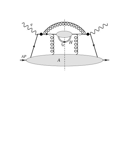
Figure 8: Two examples of twist-4 diagrams that contribute to the evolution equations of medium-modified fragmentation functions. Propagators with poles that make the gluon from the nucleus soft (momentum $\sim\xi_{D}$) are indicated by a grey circle, propagators whose poles make the gluon harder (momentum $\sim\xi_{L}$) are shown with a solid black circle. There are many more diagrams including those with different final state cuts and interference diagrams in which the gluon from the nucleus couples to different particles in amplitude and complex conjugated amplitude.

Guo and Wang showed that the hadronic tensor at the level of nuclear enhanced twist-4 receives contributions from diagrams like the ones shown in Fig. 8 where parton $b$ or $c$, or the radiated parton could scatter off an additional medium parton $d$. They computed the result from those diagrams and found

$$\frac{dW^{\mu\nu}_{(4^{\prime})}}{dz_{H}}=\sum_{abcd}\int d\xi\int\frac{dl_{T}^{2}}{l_{T}^{4}}\frac{\alpha_{s}}{2\pi}\int_{z_{c}}^{1}\frac{dz_{b}}{z_{b}}H^{\mu\nu}_{ab}(\xi,p,q,z_{b})\int_{z_{h}}^{1}\frac{dz_{c}}{z_{c}}\left(\frac{z_{c}}{z_{b}}\right)D_{c/H}\left(\frac{z_{H}}{z_{c}}\right)\\ \times\left[P_{b\to c}\left(\frac{z_{c}}{z_{b}}\right)T_{ag/A}(\xi,\xi_{L})+\delta\left(\frac{z_{c}}{z_{b}}-1\right)\Delta T_{ag/A}(\xi,l_{T}^{2})\right]\,.$$ (47)

For simplicity of notation we have assumed here that the second parton $d$ is a gluon that does not change the identity of the parton it couples to. The other cases can be treated accordingly. The twist-4 matrix elements are similar to the soft-hard matrix elements introduced in Eq. (30). If parton $a$ is a quark we have

$$T_{qg/A}(\xi,\xi_{L})=\int dy_{4}^{-}{dy_{3}^{-}}\frac{dy_{1}^{-}}{2\pi}e^{i(\xi+\xi_{L})P^{+}y_{1}^{-}}\left(1-e^{-i\xi_{L}P^{+}y_{4}^{-}}\right)\left(1-e^{-i\xi_{L}P^{+}(y_{1}^{-}-y_{3}^{-})}\right)\Theta(y_{1}^{-}-y_{3}^{-})\Theta(-y_{4}^{-})\\ \times\left\langle A(P)\right|\bar{q}(0)\gamma^{+}q(y_{1}^{-})F_{a}^{+\nu}(y_{3}^{-})F_{a\,\nu}^{\>\>\>\>+}(y_{4}^{-})\left|A(P)\right\rangle\,.$$ (48)

The expression also contains a derived matrix element

$$\Delta T_{qg/A}(\xi,l_{T}^{2})=\int_{0}^{1}\frac{dz}{1-z}\left[2T_{qg/A}(\xi,\xi_{L})|_{z=1}-(1+z^{2})T_{qg/A}(\xi,\xi_{L})\right]$$ (49)

which remains after the virtual corrections have canceled the singularity at $z=1$.

We note that the normalization of the matrix elements, that is following Guo and Wang here, differs by a factor $2\pi$ from Eq. (30). We have also gone beyond the soft-hard matrix elements by allowing parton $d$ to have a non-vanishing momentum fraction

$$\xi_{L}=\frac{l_{T}^{2}}{2P^{+}q^{-}z(1-z)}$$ (50)

with $z=z_{c}/z_{b}$. It is the structure $(1-\exp(\ldots))(1-\exp(\ldots))$ in (48) that exhibits interference and will eventually lead to the LPM effect in the Higher Twist formalism. One can easily see how this interference emerges in the calculation. The momentum of parton $d$ is fixed by the poles of partons $b$/$c$ and there are two kinematic possibilities shown in Fig. 8. Either the momentum of parton $d$ is very soft with a momentum fraction $\xi_{D}\sim k_{T}^{2}/Q^{2}$ which vanishes when its intrinsic transverse momentum $\mathbf{k}_{T}$ is set to zero. The phase $\exp(-i\xi_{D}P^{+}y^{-})$ then reduces to unity. The other pole sets the momentum fraction to $x_{L}$, and interestingly the amplitudes for both poles exhibit a relative minus sign. This interference is common when higher twist corrections are considered together with radiative corrections. A discussion of this soft-hard interference in the context of Drell-Yan can be found in [71, 72, 73, 110].

The collinear radiation corrections at twist-4 can be resummed in modified evolution equations for new fragmentation functions $\tilde{D}$ in cold nuclei just as in the twist-2 (DGLAP) case. The resulting set of equations takes exactly the same form as in Eq. (7), with $D\to\tilde{D}$ and new, medium-dependent splitting functions

$$\tilde{P}_{ab}(z)=P_{ab}(z)+\Delta P_{ab}(z)$$ (51)

where $P_{ab}$ is the usual vacuum splitting function and $\Delta P_{ab}$ is the twist-4 correction. For the case of $q\to q+g$ splitting induced by a gluon we have

$$\Delta P_{q\to q}(z)=\frac{2\pi\alpha_{s}C_{A}}{N_{c}}\frac{1}{l_{T}^{2}}\left[\left(\frac{1+z^{2}}{1-z}\right)_{+}\frac{T_{qg/A}(\xi,\xi_{L})}{f_{q/A}(\xi)}+\delta(z-1)\frac{\Delta T_{qg/A}(\xi,l_{T}^{2})}{f_{q/A}(\xi)}\right]\,.$$ (52)

The other modified splitting functions are discussed in Ref. [102] for scattering off gluons and in Ref. [111] for scattering off quarks. Even though this result is technically correct and very useful we can also see its limitations. The splitting functions, and as a consequence the modified fragmentation functions $\tilde{D}$, are no longer universal as they depend on the underlying process through the matrix elements $T$. In fact they are no longer just functions of a single momentum fraction $z$ but also depend in a non-trivial way on $\xi$. On the other hand, the breaking of universality encodes the medium effects that we are after.

The new medium-modified fragmentation functions allow us to write hadron production in $e+$A collisions in a very simple way analogous to Eq. (45) as

$$\frac{dW^{\mu\nu}_{(4)}}{dz_{H}}=\sum_{ab}\int d\xi f_{a/A}(\xi,Q)\int_{z_{H}}^{1}\frac{dz_{b}}{z_{b}}H^{\mu\nu}_{ab}(\xi,p,q,z_{b})\tilde{D}_{b/H}\left(\frac{z_{H}}{z_{b}},Q\right)\,.$$ (53)

The dependence of the $\tilde{D}$ on other quantities is usually suppressed in the notation. We have now come to a point where one has to introduce a certain amount of modeling since a rigorous solution would include a simultaneous fit of the $\tilde{D}_{ab/A}$ and the $T_{ab/A}$ in the same environment (because of the loss of universality) with the evolution equations as constraints. This is too complex a task given the available data.

The twist-4 matrix elements are modeled similar to the less general soft-hard matrix elements from Eq. (31). It seems safe to assume that $T_{ab/A}$ can be factorized into a product of two parton distributions for partons $a$ and $b$ resp. Guo and Wang model the interference effect by introducing a massless parameter for the radius $R_{A}$ of the nucleus, $x_{A}=1/(MR_{A})$, where $M$ is the mass of a nucleon. They suggest

$$T_{ab/A}(\xi,\xi_{L})\approx\frac{C}{x_{A}}\left(1-e^{-\xi_{L}^{2}/x_{A}^{2}}\right)\left[f_{a/A}(\xi)\,\xi_{L}f_{b/A}(\xi_{L})+f_{a/A}(\xi+\xi_{L})\,\kappa_{b}\right]$$ (54)

where $C$ is a normalization constant and $\kappa_{b}\approx\lim_{x\to 0}xf_{b/A}(x)$ formally is the value of the parton density for parton $b$ when it is very soft, i.e. with momentum fraction of order $x_{D}$. Obviously $\kappa_{g}$ is proportional to the gluon density $\lambda^{2}$ introduced in Eq. (34). Note that the dependence on the size of the system is hidden in $x_{A}$ and the leading size dependence is $\sim A^{1/3}$. On the other hand the formation time of the radiation is $\sim 1/(x_{L}P^{+})$ and the factor $1-e^{-\xi_{L}^{2}/x_{A}^{2}}$ leads to LPM suppression unless $\xi_{L}\gg x_{A}$. In Ref. [113] the authors suggest an even simpler model that drops the second term

$$T_{ab/A}(\xi,\xi_{L})\approx\frac{\tilde{C}_{b}}{x_{A}}\left(1-e^{-\xi_{L}^{2}/x_{A}^{2}}\right)f_{a/A}(\xi)\,.$$ (55)

Even if the set of twist-4 matrix elements were perfectly known there is still the task to extract the medium-modified fragmentation functions from the set of evolution equations. Guo and Wang originally suggested the first iteration

$$\tilde{D}_{a/H}(z,\mu)=D_{a/H}(z,\mu)+\frac{\alpha_{s}}{2\pi}\int_{0}^{\mu^{2}}\frac{dl_{T}^{2}}{l_{T}^{2}}\int_{z}^{1}\frac{dy}{y}\sum_{b}\Delta P_{a\to b}(y)D_{b/H}\left(\frac{z}{y}\right)$$ (56)

as an approximate solution. Note that the $\Delta P_{a\to b}$ carry all the information about the medium through Eq. (52) and its counterparts. Deng and Wang recently showed how to solve modified evolution equations numerically [112].

Using the first iteration the energy loss of a parton can be calculated as the shift in the momentum fraction due to the term $\Delta P_{a\to b}$ in the equation above

$$\langle\Delta y\rangle=1-\frac{\alpha_{s}}{2\pi}\int_{0}^{\mu^{2}}\frac{dl_{T}^{2}}{l_{T}^{2}}\int_{z}^{1}{dy}\sum_{b}\Delta P_{a\to b}(y)\,.$$ (57)

For quarks one finds [87, 113]

$$\langle\Delta y\rangle=\tilde{C}_{g}\frac{\alpha_{s}^{2}C_{A}}{N_{c}}\frac{6x_{B}}{Q^{2}}\frac{1}{x_{A}^{2}}(-\ln 2x_{B})$$ (58)

which is proportional to the nuclear size squared, $\langle\Delta y\rangle\propto A^{2/3}$, as expected for the LPM regime. $x_{B}=Q^{2}/(2P^{+}q^{-})$ is the Bjorken variable in deep inelastic scattering. In Ref. [113] the authors can explain the observed suppression of semi-inclusive hadron production in the HERMES experiment [114] very well using the medium modified fragmentation functions described above. One can go one step further and try to interpret the medium modification as a simple rescaling of the vacuum fragmentation functions. One uses an ansatz [113, 115]

$$\tilde{D}_{a/H}(z)\approx\frac{1}{1-\Delta z}D_{a/H}\left(\frac{z}{1-\Delta z}\right)$$ (59)

where $\Delta z$ is the typical energy loss for parton $a$. This formula can only be a satisfying approximation in a limited region with $z+\Delta z<1$. At this level the medium-modified fragmentation functions have been cast in a very general form and one can try to apply the general concepts to systems other than $e+$A. In particular one can extract the stopping power $\langle\Delta E/L\rangle\approx E\Delta z/L$ for a particle with initial energy $E$ from data in heavy ion collisions. Using the techniques here (and including the dilution of the medium through the longitudinal expansion in nuclear collisions) E. Wang and X.N. Wang concluded in 2002 that the differential energy loss extracted from data in Au+Au collisions at RHIC was about 15 times larger than the one for cold nuclear matter measured at HERMES [113].

Beyond the first iteration, Deng and Wang have systematically studied the evolution of gluon induced parton-to-parton fragmentation functions (starting from $D_{a/a}=\delta(z-1)$ and $D_{a/b}=0$, $b\neq a$ initial conditions at a low scale). They also investigate the energy and medium thickness dependence and apply their techniques to pion fragmentation with parameterized vacuum fragmentation functions as input. Modified evolution suppresses the fragmentation functions at intermediate and large values of $z$ as expected [112].

In recent years progress was made on the HT formalism (in its original meaning for deep-inelastic scattering) by considering medium modifications for double fragmentation [116], elastic energy loss [117] and through successful resummation of multiple scatterings per photon or gluon emission [79, 118].

2.3.3 The AMY Formalism

The particular merit of the formalism widely know as AMY, after Arnold, Moore and Yaffe, is its complete internal consistency in a very high temperature regime. The basic picture is the following. Partons propagating through a plasma with temperature $T$, themselves having momenta of order $T$ or larger but small virtualities, interact perturbatively with quarks and gluons in the plasma with thermal masses $\sim gT$. They pick up transverse momentum of the same order $gT$, and then radiate gluons (for quarks) or split into quark-antiquark pairs or two gluons (for gluons), again at typical transverse momentum scales $gT$. This leads to formation times that are rather long, of the order $T/(gT)^{2}\sim 1/(g^{2}T)$. The shortcomings are the requirements of small initial off-shellness of the parton, an unlikely condition for a parton emerging from a hard process, and the condition of very small coupling $g\ll 1$ to justify thermal perturbation theory, which requires very large temperatures $T\gg T_{c}$. The exact temperature from which on such calculations start to be reliable is a matter of debate. One must also assume that the temperature does not change during the formation time of radiation which is questionable for rapidly evolving fireballs. Nevertheless, the rigor of the formalism has made AMY an appealing choice in the canon of energy loss calculations.

The AMY formalism grew out of a computation of the complete leading order, hard thermal loop (HTL) resummed perturbative photon and gluon emission rates. Arnold, Moore and Yaffe introduced, for the first time, the correct treatment of collinear emission in a finite temperature medium, which must take into account the LPM effect due to the long formation times $\sim 1/(g^{2}T)$ [52, 53, 103]. The applications of these results to photon production in quark gluon plasma had been mentioned in a previous section. The results for gluon radiation off a parton with typical momentum $T\gg gT$ in the medium can be used to calculate its rate of energy loss. For quarks of momentum $p$ radiating gluons of momentum $k$ the rate is [103, 104]

$$\frac{\partial\Gamma_{q\to qg}}{\partial k\partial t}(p,p-k)=\frac{C_{R}\alpha_{s}}{4p^{7}}n_{B}(k)n_{F}(p-k)\frac{1+(1-x)^{2}}{x^{3}(1-x)^{2}}\int\frac{d^{2}h}{(2\pi)^{2}}2\mathbf{h}\cdot\mathrm{Re}\,\mathbf{F}(\mathbf{h},p,k)$$ (60)

where $n_{B}$ and $n_{F}$ are the boson and fermion occupation factors for the gluon and the quark in the final state, $x=k/p$ is the momentum fraction of the gluon, and $\mathbf{h}=\mathbf{p}\times\mathbf{k}$ is a useful measure for the non-collinearity of the final state. $\mathbf{F}\propto\mathbf{h}$ is a function defined by the integral equation

$$2\mathbf{h}=i\delta E(h,p,k)\mathbf{F}(\mathbf{h})+\frac{\alpha_{s}}{2\pi}\int d^{2}q_{\perp}V({q}_{\perp})\times\left[(2C_{R}-C_{A})\left(\mathbf{F}(\mathbf{h})-\mathbf{F}(\mathbf{h}-k\mathbf{q}_{\perp})\right)\right.\\ +\left.C_{A}\left(\mathbf{F}(\mathbf{h})-\mathbf{F}(\mathbf{h}+p\mathbf{q}_{\perp})\right)+C_{A}\left(\mathbf{F}(\mathbf{h})-\mathbf{F}(\mathbf{h}-(p-k)\mathbf{q}_{\perp})\right)\right]\,.$$ (61)

We have dropped the second and third argument in $\mathbf{F}(\mathbf{h},p,k)$ for brevity, in all cases above they are equal to the initial momentum $p$ and the radiated momentum $k$ resp. It is the function $\mathbf{F}$ that encodes important properties of the medium via the potentials

$$V({q}_{\perp})=\frac{m_{D}^{2}}{q_{\perp}^{2}(q_{\perp}^{2}-m_{D}^{2})},\qquad m_{D}^{2}=\frac{g^{2}T^{2}}{6}(2N_{c}+N_{f})$$ (62)

as a function of momentum transfer $\mathbf{q}_{\perp}$ and temperature $T$.

$$\delta E(h,p,k)=\frac{h^{2}}{2pk(p-k)}+\frac{m_{k}^{2}}{2k}+\frac{m_{p-k}^{2}}{2(p-k)}-\frac{m_{p}^{2}}{2p}$$ (63)

is the energy difference between final and initial state. The masses $m$ are $m_{D}/\sqrt{2}$ for gluons and $gT/\sqrt{3}$ for quarks in the respective channels with momenta $p$, $k$ and $p-k$.

The rates for other processes can be obtained from Eq. (60) by replacing the splitting functions, adjusting the Bose or Fermi factors, and putting the correct color factor $C_{R}$. The missing splitting functions needed are

$$N_{f}\frac{x^{2}+(1-x)^{2}}{x^{2}(1-x)^{2}} \quad\mathrm{for}\,g\to q\bar{q}\,,$$ (64)

$$\frac{1+x^{4}+(1-x)^{4}}{x^{2}(1-x)^{3}} \quad\mathrm{for}\,g\to gg\,.$$ (65)

The rates for different processes as a function of time $t$ can be implemented in coupled rate equations for quark, antiquark, and gluon momentum distributions $f_{q}$, $f_{\bar{q}}$ and $f_{g}$ resp.

$$\frac{f_{q}(p)}{\partial t} =\int_{-\infty}^{\infty}dk\left[\frac{\partial\Gamma_{q\to qg}(p+k,k)}{\partial k\partial t}f_{q}(p+k)-\frac{\partial\Gamma_{q\to qg}(p,k)}{\partial k\partial t}f_{q}(p)+\frac{\partial\Gamma_{g\to q\bar{q}}(p+k,k)}{\partial k\partial t}f_{g}(p+k)\right]\,,$$ (66)

$$\frac{f_{g}(p)}{\partial t} =\int_{-\infty}^{\infty}dk\left[\frac{\partial\Gamma_{q\to qg}(p+k,p)}{\partial k\partial t}\left(f_{q}(p+k)+f_{\bar{q}}(p+k)\right)-\frac{\partial\Gamma_{g\to q\bar{q}}(p,k)}{\partial k\partial t}f_{g}(p)\right.$$

$$\qquad\qquad\left.+\frac{\partial\Gamma_{g\to gg}(p+k,k)}{\partial k\partial t}f_{g}(p+k)-\frac{\partial\Gamma_{g\to gg}(p,k)}{\partial k\partial t}f_{g}(p+k)\Theta(2k-p)\right]\,.$$ (67)

The equation for the antiquark distribution is analogous to the equation for the quark distribution. Note that the emitted momentum $k$ can be positive or negative, which means that a parton can in principle also acquire momentum from the medium. Of course, a parton with momentum much larger than typical thermal momenta will still lose momentum on average. Final quark and gluon spectra can be subjected to vacuum fragmentation to compute final hadron spectra.

2.3.4 The GLV Formalism

The GLV energy loss model by Gyulassy, Levai and Vitev [107, 108, 109] is based on the earlier Gyulassy-Wang model. It describes the medium as an ensemble of static scattering centers with Yukawa potentials exhibiting a screening mass $\mu$, which also set the typical scale of transverse momentum transfer. The scattering amplitude is then expanded in terms of the opacity $L/\lambda$ where $L$ is the length of the medium and $\lambda$ is the mean free path. The leading, zeroth order term, for a parton with energy $E$ corresponds to vacuum radiation with a spectrum

$$\frac{dI^{(0)}}{dxdk^{2}}=\frac{C_{R}\alpha_{s}}{2\pi}\left(2-2x+x^{2}\right)E\frac{1}{k^{2}}$$ (68)

as a function of the gluon longitudinal momentum fraction $x$ and transverse momentum $\mathbf{k}$. $C_{R}$ is the color Casimir factor in the appropriate representation, $C_{F}=4/3$ for quarks and $C_{A}=3$ for gluons.

At the next order in opacity one considers the interference of vacuum radiation and a single medium-induced radiation with momentum transfer $\mathbf{q}$ [109]

$$\frac{dI^{(1)}}{dxdk^{2}}=\frac{C_{R}\alpha_{s}}{2\pi}\left(2-2x+x^{2}\right)\frac{L}{\lambda}E\frac{1}{k^{2}}\,\int d^{2}q\frac{\mu^{2}}{\pi(q^{2}+\mu^{2})^{2}}\frac{\mathbf{k}\cdot\mathbf{q}(\mathbf{k-q})^{2}L^{2}}{16x^{2}E^{2}+(\mathbf{k-q})^{4}L^{2}}\,.$$ (69)

The integrals can be evaluated analytically away from the extreme cases $x\to 0$ and $x\to 1$. Then maximally loose kinematic constraints $0<k<\infty$, $0<q<\infty$ can be assumed and the total energy loss at first order in opacity is

$$\Delta E^{(1)}=\frac{C_{R}\alpha_{s}}{4}\frac{\mu^{2}}{\lambda}L^{2}\ln\frac{E}{\mu}\,.$$ (70)

It exhibits the characteristic $L^{2}$-dependence. In contrast the zeroth order gluon spectrum (68) will lead to a “vacuum quenching”

$$\Delta E^{(0)}=\frac{4C_{R}\alpha_{s}}{3\pi}E\ln\frac{E}{\mu}$$ (71)

where $\mu$ in this case is chosen to play the role of a lower cutoff for the transverse momentum $k$.

Higher orders in the opacity $(L/\lambda)^{n}$ can be treated numerically [109]. Since the number of emitted gluons is finite, fluctuations around a given mean value are important. They can be taken into account through Poisson statistics [119], leading to a probability distribution $P(\epsilon)$ for the fractional energy loss $\epsilon=\Delta E/E$. The probabilities for emission of $n$ gluons are

$$P_{n}(\epsilon)=\frac{e^{-\bar{N}_{g}}}{n!}\prod_{i=1}^{n}\int dx_{i}\frac{dI}{dx_{i}}\delta\left(\sum_{i}x_{i}-\epsilon\right)$$ (72)

where $\bar{N}_{g}$ is the average number of gluons and $dI/dx$ is the gluon energy spectrum to the desired order in opacity, e.g. derived from Eq. (69) to first order. The total probability distribution is

$$P(\epsilon)=\sum_{n=1}^{\infty}P_{n}(\epsilon)\,.$$ (73)

It can be used to define a medium-modified fragmentation function

$$D^{\mathbf{GLV}}_{a/H}(z,Q)=\int_{0}^{1}d\epsilon\frac{P(\epsilon)}{1-\epsilon}D_{a/H}\left(\frac{z}{1-\epsilon},Q\right)\,$$ (74)

analogous to Eq. (59). Recall that we tacitly assume that parton energy loss and the actual hadronization of the parton are factorizable, and hadronization itself happens outside of the medium. There have also been attempts to include elastic scattering consistently in the GLV approach [120, 121].

2.3.5 The ASW Formalism

The energy loss model due to Armesto, Salgado and Wiedemann [105, 106] assumes a Poisson-like distribution of gluon emissions as described in Eqs. (72) and (73). The proponents of the model present a resummed version of the so-called quenching weight $P$. They add the explicit possibility $P_{0}$ of zero gluon emissions, i.e. a finite probability that a parton escapes unquenched. For their main result they use the gluon radiation spectrum $dI/dx$ from the BDMPS approach assuming finite propagation length $L$ [95, 96, 97, 98, 122]. They also present results for a resummation of gluon spectra in a GLV-like opacity expansion [123], but we will not discuss that latter option in detail.

In the case of BDMPS soft scattering they introduce a characteristic gluon frequency

$$\omega_{c}=\frac{1}{2}\hat{q}L^{2}$$ (75)

and a dimensionless quantity

$$R=\omega_{c}L\,.$$ (76)

Note that $\omega_{c}$ is close to the definition in Eq. (41). $R$ is introduced to enforce the kinematic constraint $k_{\perp}<\omega$. From its definition we can infer that $R\to\infty$ corresponds to an infinitely large medium if $\omega_{c}$ is finite. It is also the limit in which the previous BDMPS result is recovered.

One can perform a numerical resummation of the Poisson sum $P$ from Eq. (73) for $n>0$. The total probability is then written as a sum

$$P(\Delta E)=p_{0}(\omega_{c},R)\delta(\Delta E)+p(\Delta E,\omega_{c},R)\,$$ (77)

which contains a discrete probability $p_{0}$ for zero energy loss and the resummed probability for finite energy loss ($n>0$). The unphysical case $\Delta E>E$ can be dealt with by either renormalizing the total probability to unity (“reweighted”) or by introducing a second $\delta$-function at $\Delta E=E$ which accumulates the probability for total loss of the jet (“non-reweighted”) [122, 124]. The uncertainty in the treatment of the case $\Delta E>0$ leads to a rather large uncertainty in describing the data, see e.g. Fig. 22. The authors of the ASW model provide a Fortran code which computes both the discrete and the continuous part of the quenching weight as functions of $\Delta E/\omega_{c}$ and $R$ [125]. As in the GLV case the quenching weights can be used to define modified fragmentation functions using Eq. (74), although also in the ASW case the true, non-perturbative fragmentation process itself is considered independent and not affected by the medium.

For applications in heavy ion collisions we need a way to go beyond the simple assumptions of a homogeneous medium in which $\hat{q}$ is constant along the propagation path of the parton. In fact in a realistic fireball $\hat{q}=(\mathbf{x},t)$ where $\mathbf{x}$ is the position in the fireball and $t$ the time. The extraction of $\hat{q}=(\mathbf{x},t)$, or at least a spatially and time-averaged version $\langle\hat{q}\rangle$ of it, is actually the goal of the hard probes program. One can deduce $\omega_{c}$ and $R$ from the two lowest moments of $\hat{q}$ integrated over the path of a jet particle,

$$I_{n}=\int_{0}^{\infty}\hat{q}\left(\mathbf{x}(t),t\right)|\mathbf{x}(t)-\mathbf{x}_{0}|^{n}dt\,.$$ (78)

Here $\mathbf{x}(t)$ is the trajectory of the particle originating from a point $\mathbf{x}_{0}$ at $t=0$ (the integrals can also be shifted by a finite formation time). Then we have

$$\omega_{c}=I_{1}\,,\qquad R=\frac{2I_{1}^{2}}{I_{0}}\,.$$ (79)

Due to the sheer impossibility to extract detailed space-time information on $\hat{q}$ it has become standard to assume that $\hat{q}$ is locally proportional to a quantity whose distribution and time-evolution is approximately known. A popular choice is the $3/4$th power of the local energy density $\epsilon$

$$\hat{q}(\mathbf{x},t)=2K\epsilon^{3/4}(\mathbf{x},t)\,,$$ (80)

or the entropy density $s$. This is the parametric dependence expected from dimensionality arguments for a fully thermalized quark gluon plasma [126]. $K$ is then treated as a fit parameter and we expect it to be close to unity for a weakly coupled plasma and larger for a strongly coupled system. Other choices for modeling the shape of $\hat{q}$ found in the literature are the temperature $T(\mathbf{x},t)$ of an equilibrated plasma, and the density of the number of participant nucleons or number of binary nucleon-nucleon collisions, which are then usually treated as time-independent medium distributions.

2.3.6 Final State Effects: Other Developments

We want to end the discussion of final state effects in nuclear collisions by briefly touching upon two special topics. We have mostly focused our attention on the production of hadrons since this is the dominant mode of measurement at RHIC. At LHC, the calorimetric measurements of jets will become much more important as their energy grows much above the background event. The advent of fast and reliable jet algorithms for high-multiplicity environments [127, 128, 129] has added to the excitement.

One possible way of modeling jets is through advanced Monte Carlo simulations of medium induced gluon radiation that does not just focus on the leading parton but tracks the evolution of the entire parton shower. Monte Carlo jet quenching modules like PYQUEN [130], Q-PYTHIA [131], JEWEL [132] , YaJEM [133] and MARTINI [134] have made progress in that direction. Another approach is the study of jet shapes in heavy ion environments that track the flow of energy through cones of given radius [135]. These studies will be much more flexible and comprehensive than leading hadron studies as they give much better answers to the question of “energy loss” which is, of course, rather a redistribution of energy than a real loss.

Another interesting field that has emerged in recent years is the study of hadron chemistry in jets. A heavy ion environment not only redistributes energies of energetic particles, it can also lead to significant changes in the relative abundances of hadrons. This can either happen through profound changes in the way hadronization works in high multiplicity environments [136], see also the discussion on quark recombination in the next section, or through the exchange of particles with the quark gluon plasma which leads to a phenomenon termed jet conversion [137, 138, 139, 140]. Jet conversions would increase the number of protons and kaons relative to pions in nuclear collisions vs $p+p$ collisions. In the former case constantly occurring conversions between quarks and gluons wash out the different color factors for their respective suppression, leading to equal suppression of particles from light quark and gluon fragmentation. In the later case the small sample of high-$p_{T}$ strange quarks is tremendously enhanced relative to up and down quarks when quenched in a chemically equilibrated quark gluon plasma. In Ref. [138] the authors predicted a factor 2 increase in the $R_{AA}$ of kaons vs pions which seems to bee seen in preliminary STAR data [141].

Conversions have been particularly well understood in the case of photons [142, 143, 144] and dileptons [145, 146]. Both induced photon bremsstrahlung [52, 97] and elastic annihilation and Compton scattering with the medium ($q+\bar{q}\to\gamma+g$ and $q+g\to\gamma+q$ resp.) lead to photon yields that are comparable with other sources (thermal, hard direct, vacuum bremsstrahlung) at intermediate transverse momenta of a few GeV/$c$. Both the evolution equations of the Higher Twist formalism and the rate equation of AMY can accommodate more channels and “flavor” changing processes in a straight forward manner to study these effects.

2.4 The Perturbative Approach: Critique and Challenges

Despite the large amount of effort put into the development of a perturbative description of hadron production in heavy ion collisions, there are uncertainties remaining about the exact nature of jet-medium interactions in the kinematic and temperature regimes important at RHIC. We will discuss in more detail in Sec. 4 below that the four approaches described here generally fare well in describing RHIC data, but they can reach very different quantitative conclusions about the quenching strength $\hat{q}$. This should not come as a big surprise since the approaches differ in some of their basic assumptions, and there are large uncertainties in modeling hard probes beyond the calculation of an energy loss rate for a quark or gluon.

Currently the big picture can be summarized as follows: perturbative calculations under various assumptions are compatible with RHIC data, but the constraints are insufficient to rule out any of the models. The experimental constraints are also insufficient to completely exclude non-perturbative mechanisms of jet quenching. Calculations using the AdS/CFT correspondence to model strongly interacting QCD [147, 148, 149] can describe the same basic phenomenology. Most likely this challenge to perturbative QCD can only be answered at LHC. The extrapolation of jet quenching to larger jet energies is significantly different in strong coupling and perturbative scenarios [150]. It is also possible to imagine a small regime of strong non-perturbative quenching around $T_{c}$ together with perturbative quenching at higher temperatures. Such mixed scenarios might be hard to distinguish experimentally. One such picture was recently explored by Liao and Shuryak [151]. They found that a “shell”-like quenching profile in which quenching is enhanced around $T_{c}$ can give better simultaneous fits to single hadron suppression and elliptic flow.

Table 1: pQCD-based energy loss models: This table summarizes some of the key assumptions of the four perturbative calculations discussed here. The models differ with respect to the medium (thermalized, perturbative), kinematics, scales ($E$ = energy of the parton, $k_{T}$ = transverse momentum of the emitted gluon, $\mu$ = typical transverse momentum picked up from the medium, $T$ = temperature, $\Lambda$ = typical momentum scale of a (non-thermalized) medium, $x$ = typical momentum fraction of the emitted gluon), and the treatment of the resummation.

Model	Assumptions about the Medium	Scales	Resummation
GLV	static scattering centers (Yukawa), opacity expansion	$E\gg k_{T}\sim\mu$, $x\ll 1$	Poisson
ASW	static scattering centers, multiple soft scattering (harmonic oscillator approximation)	$E\gg k_{T}\sim\mu$, $x\ll 1$	Poisson
HT	arbitrary matrix element at scale $\Lambda$ (thermalized or non-thermalized medium)	$E\gg k_{T}\gg\Lambda\sim\mu$	DGLAP
AMY	perturbative, thermal, $g<<1$ (asymptotically large $T$)	$E>T\gg gT\sim\mu$	Fokker-Planck

Additional uncertainties come from a variety of issues regarding the details of the phenomenological modeling:

• The initial state: Jets will interact with their environment before a quark gluon plasma is fully formed. The time dependence of $\hat{q}$ during the first fm/$c$ of the collisions is highly uncertain, in particular if initial interactions are dominated by coherent gluon fields [20, 21]. Some calculations set an ad-hoc start time or use different extrapolations to small times. One estimate of uncertainties can be found in [152] and is discussed in more detail in Fig. 40 below.

• Fireball evolution: Wildly different fireball parameterizations used in jet quenching calculations can be found in the literature up to this day. The correct longitudinal and transverse expansion with the correct cooling rate have to be taken into account. Recently comparisons of different calculations using the same underlying fireball calculated from hydrodynamics have become available [153]. However, as we will discuss in detail in the Sec. 3, uncertainties remain in hydrodynamic calculations as well which are transferred to hard probes when hydrodynamics is used as a background.

• The hadronic phase: The models referenced here deal with parton energy loss in a partonic medium. Clearly a jet will also interact with a surrounding hadronic medium. Some models could in principle deal with this situation (e.g. the higher twist approach only needs the jet to be dominated by a sufficiently high energy parton), others have to fail (like the AMY approach). But none of them addresses the question of fully formed high energy hadrons in a jet interacting with a hadronic medium. Shower simulations with full space-time evolution might be helpful to constrain at least the size of the problem from the partonic side.

• Event-by-event fluctuations: Not much is known from experiment about spatial fluctuations in the fireball, but clearly we should expect a fireball to exhibit a certain degree of inhomogeneity as suggested by many models of initial nucleus-nucleus interactions. Compared to quenching in a smooth, average fireball, event-by-event quenching can lead to considerably different results for hadron suppression and elliptic flow [154].

• Back-reaction from the medium: While the medium modifies jets, jets on the other hand modify the surrounding medium by transferring energy and momentum. The heating of the medium can be considerable [155], and a variety of shock phenomena can occur [156, 157, 158]. Clearly, a comprehensive approach will consider both the jet and the medium as variable and would not fix one or the other as a background or boundary condition. In particular, if part of the energy (or maybe most of the energy for some jets) thermalizes, this most likely proceeds through non-perturbative channels which are not included in either of the models discussed here.

There are no systematic studies of all uncertainties together. A pessimistic estimate of their compounded effect would be a factor 3-5 uncertainty in the extraction of $\hat{q}$ from RHIC data.

Let us finally revisit the four approaches to calculate leading particle energy loss discussed here. Why do they lead to similar qualitative, but sometimes quite different quantitative results? We have discussed the underlying assumptions of each model in its respective section. We summarize them once more in Tab. 1 in terms of the different ways the medium is modeled, the hierarchy of scales and the way resummation is handled. Two key points are the different assumptions about the transverse momentum $k_{T}$ of the emitted gluon vs the transverse momentum $\mu$ picked up from the medium, and the philosophy of multiple soft emissions vs an opacity expansion (with single, somewhat larger transverse kicks). The full solution of the problem is quite complex, even in a fully perturbative medium. We refer the interested reader to the recent assessment by Arnold [159] and the review by Majumder and Van Leeuwen [99]. It might be a while until more comprehensive calculations are available, but efforts in this direction are under way, e.g. within the TECHQM and JET collaborations. Simplistic assumption have to be improved and narrow kinematic regimes have to be widened.

3 Success of Hydrodynamic Models at RHIC

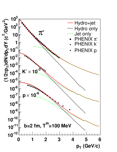
Figure 18: Spectra from hydrodynamics (dotted), pQCD (dash-dotted), and their sum (solid line) for $\pi^{-}$, $K^{-}$, and $p$ in Au+Au collisions at $\sqrt{s_{NN}}=200$ GeV for impact parameter $b=2.0$ fm compared to data from PHENIX [273]. Figure reprinted from [268] with permission from the American Physical Society.

Since Landau [160] and Bjorken [161] proposed the idea to apply hydrodynamics to the production of particles in high energy collisions, it has evolved into one of the most useful phenomenological models for our understanding of high energy heavy ion collisions. Starting with Landau’s hydrodynamic description and Bjorken’s scaling solution, various kinds of implementations of hydrodynamics were developed to understand experimental data from the Alternating Gradient Synchrotron (AGS) and and the Super Proton Synchrotron (SPS). Hydrodynamics and hydro-inspired models (e.g. the Blast-Wave Model [162]) give us reasonable explanations for a large amount of experimental data: single particle spectra (with respect to transverse momentum $P_{T}$ and pseudorapidity $\eta$), two particle correlations, collective flow, and electromagnetic probes. However they did not appear to work for some aspects of anisotropic flow, e.g. directed flow $v_{1}$ and anisotropic flow $v_{2}$. For example, the rapidity dependence of directed flow of charged pions is different from that of protons [163, 164]. The charged pion $v_{1}$ decreases with rapidity, but the proton $v_{1}$ increases (see Figs. 18 and 19 in Ref. [164]). This difference between pions and protons is difficult to understand from collectivity arguments which is one of the crucial features of hydrodynamics. To explain this interesting behavior in detail, hydrodynamics may be too simplistic and additional effects may play a role. Therefore transport models in which more complicated dynamics of the underlying theory are included fare better for directed flow. Another hint comes from the fact that hydrodynamic models routinely overestimate the size of elliptic flow at SPS energies [164]. This suggests that the system does not completely equilibrate. Hence the validity of hydrodynamics at SPS energies is not very clear. This led to the pre-RHIC view that hydrodynamic models were rather simple-minded phenomenological tools.

All of this changed dramatically after the first experimental results from RHIC came out in 2000. Hydrodynamic models could naturally explain the unexpectedly large elliptic flow at RHIC compared to that at SPS [165, 166]. The success of hydrodynamics at RHIC, together with observations of jet quenching in the medium many times larger than that in cold nuclear matter, indications for the existence of a Color Glass Condensate and the success story of recombination models, are cited as the main results from the RHIC program, as evidence for production of a quark gluon plasma with deconfined partons, and for the conjecture that this QGP is strongly coupled (a “sQGP”) and in fact may be the most perfect liquid ever seen [4, 167].

In the wake of this success hydrodynamics has become the most promising tool to describe most of the expansion and cooling process of the bulk of the matter created in heavy ion collisions at RHIC. However, at the same time limitations of hydrodynamic models, old ones and novel ones, were found: e.g. the failure to describe experimental data on two-particle correlations, or elliptic flow as a function of pseudorapidity. This suggests that the assumption of perfect fluidity is not valid for the entire fireball at RHIC. At least in the hadronic phase and in the final state viscous effects can not be neglected [168]. Since the perfect fluidity hypothesis is tested through precision analyses of elliptic flow [169] one needs to overcome this obstacles with hybrid models that couple hydrodynamics to hadron-based transport models and through the development of viscous hydrodynamic codes.

Both of those avenues have undergone remarkable developments in recent years. In particular our understanding of second order viscous, relativistic hydrodynamics has increased tremendously over the past few years. While the extraction of the equation of state for quark gluon plasma and the phase transition used to be at the forefront of hydrodynamic modeling, the extraction of transport coefficients, like shear and bulk viscosity, of the hot and dense matter created at RHIC has been added to the main goals. In this section we will review the basic principles and numerical concepts of hydrodynamics together with some recent progress. We will then discuss applications of hydrodynamic models at RHIC.

3.1 Basics of Relativistic Hydrodynamics

3.1.1 The Framework of Ideal Hydrodynamics

Let us start with the ideal relativistic hydrodynamic equations of motion. In ideal hydrodynamics thermalization is perfect and there is a well-defined local rest frame for each fluid cell. In that local rest frame, the energy-momentum tensor of a volume element of the fluid (where Pascal’s law works) is given by

$$\tilde{T}^{\mu\nu}(x)=\left(\begin{array}[]{cccc}\epsilon(x)&0&0&0\\ 0&p(x)&0&0\\ 0&0&p(x)&0\\ 0&0&0&p(x)\\ \end{array}\right)$$ (81)

where $\epsilon(x)$ and $p(x)$ are energy density and pressure, respectively, as functions of the space-time point $x^{\mu}$ of the fluid cell. Introducing the four-velocity $u^{\mu}(x)$ of each fluid cell in the lab frame we can boost the local energy-momentum tensor into the laboratory frame which gives us the well-known result

$$T^{\mu\nu}(x)=[\epsilon(x)+p(x)]u^{\mu}(x)u^{\nu}(x)-p(x)g^{\mu\nu}\,.$$ (82)

The motion of the fluid is simply described by the equations of energy and momentum conservation,

$$\partial_{\mu}T^{\mu\nu}(x)=0\,,$$ (83)

from which the entropy current conservation,

$$\partial_{\mu}(su^{\mu})=0$$ (84)

is derived. Other conserved currents $j^{\mu}(x)$ besides energy and momentum — most importantly the baryon current $j_{B}^{\mu}(x)$ — can be taken into account by imposing the conservation laws

$$\partial_{\mu}j^{\mu}(x)=0\,.$$ (85)

In ideal hydrodynamics each of these conserved currents can be written as

$$j^{\mu}(x)=n(x)u^{\mu}(x)$$ (86)

where $n(x)$ is the density of the corresponding conserved charge in the local rest frame of a fluid cell. (83) and (85) are the equations of motion that need to be solved. An equation of state (EoS) $p=p(\epsilon)$ is the last equation needed to close the system of equations. It is the only place where the underlying dynamics of the system comes into play. In practical applications the only current usually considered in heavy ion physics is the net-baryon current $j_{B}^{\mu}$. Even that current is often negligible at RHIC and LHC.

The equation of state gives us direct information about the QCD phase diagram. This direct link to the main goal of the RHIC program is one of the outstanding features of hydrodynamic models. Most hydrodynamic computations use an EoS with a first-order phase transition based on the Bag Model. However, recent lattice QCD results suggest that the phase transition at low baryon densities is rather a smooth crossover [170, 171]. Since then parameterizations of the EoS from lattice QCD have become fashionable. We will describe the recent developments in this area in more detail in Sec. 3.2.3.

3.1.2 Dissipative Corrections

When we start to include effects of dissipation into relativistic hydrodynamics, we are confronted with a rather complicated situation. One of the difficulties is that a naive introduction of viscosities causes the first order theory (i.e. first order in gradients) to exhibit acausalities. Heat might propagate instantaneously because of the parabolic character of the equations. This problem is unique to the relativistic generalization of viscous hydrodynamics. In order to avoid this problem, second order terms in heat flow and viscosities have to be included in the expression for the entropy [172, 173, 174, 175, 176, 177, 178], but the systematic treatment of these second order terms is difficult. Although there is remarkable progress toward the construction of a fully consistent relativistic viscous hydrodynamic theory there are still ongoing discussions about the correct formulation of the equations of motion and about the appropriate numerical procedures [179].

The basic tenet that has to be given up in dissipative hydrodynamics is the assumption of a uniquely defined local rest frame. Away from equilibrium the vectors defining the flows of energy, momentum and conserved currents might be misaligned. We can still define a local rest frame by just choosing a velocity $u^{\mu}(x)$ in the lab frame. Then the energy-momentum tensor and the conserved current take the more general shape

$$T^{\mu\nu}(x) =[\epsilon(x)+p(x)+\Pi(x)]u^{\mu}(x)u^{\nu}(x)-[p(x)+\Pi(x)]g^{\mu\nu}+2W^{(\mu}u^{\nu)}+\pi^{\mu\nu}\,,$$ (87)

$$j^{\mu}(x) =n(x)u^{\mu}+V^{\mu}\,,$$ (88)

where $V^{\mu}$ and $W^{\mu}$ are corrections to the flow of conserved charge and energy that are orthogonal to $u^{\mu}$ and $T^{\mu\nu}u_{\nu}$ resp., $\pi^{\mu\nu}$ (with the orthogonality conditions $u_{\mu}\pi^{\mu\nu}=\pi^{\mu\nu}u_{\nu}=0$) is the symmetric, trace-less shear stress tensor, and $\Pi$ is the bulk pressure. $(\ldots)$ around indices indicate symmetrization. Usually $u^{\mu}$ is chosen to define one of two standard frames: the Eckart frame where the velocity is given by the physical flow of net charge (then $V^{\mu}=0$), or the Landau frame where the velocity is given by the energy flow (then $W^{\mu}=0$). We refer the reader to the article by Muronga and Rischke for further details [180].

At first order the new structures have to be proportional to gradients in the velocity field $u^{\mu}$, and only three proportionality constants appear in these relations: the shear viscosity $\eta$, the bulk viscosity $\zeta$ and the heat conductivity $\kappa$. These transport coefficients are the fundamentally new quantities in dissipative hydrodynamics. With the usual definitions the first order relations in the Landau frame are [180]

$$\Pi =-\zeta\nabla_{\mu}u^{\mu}$$ (89)

$$q^{\mu} =-\kappa\frac{nT^{2}}{e+p}\nabla^{\mu}\frac{\mu}{T}$$ (90)

$$\pi^{\mu\nu} =2\eta\nabla^{<\mu}u^{\nu>}\,.$$ (91)

Here $q^{\mu}=-(\epsilon+p)/n\,V^{\mu}$ is the heat flow in the Landau frame, $\nabla^{\mu}=(g^{\mu\nu}-u^{\mu}u^{\nu})\partial_{\nu}$ is the covariant derivative orthogonalized to the flow vector, $T$ and $\mu$ are temperature and chemical potential for the conserved current resp., and $\langle\cdots\rangle$ refers to a symmetrization of indices with the trace subtracted. The entropy current $S^{\mu}$ receives additional contributions beyond the equilibrium term $su^{\mu}$ and one can show that with all three transport coefficients positive the entropy is strictly non-decreasing, $\partial_{\mu}S^{\mu}\geq 0$.

At second order many more new parameters, related to relaxation phenomena, appear. Currently, most viscous hydrodynamic calculations use the relativistic dissipative equations of motion that were derived phenomenologically by Israel and Stewart [175] and variations of those, while some use the method by Öttinger and Grmela [176, 177, 178], see e.g. [181]. Recently, a second-order viscous hydrodynamics from AdS/CFT correspondence was derived [182], as well as a set of generalized Israel-Stewart equations from kinetic theory via Grad’s 14-momentum expansion which have several new terms [183]. On the other hand however, a stable first-order relativistic dissipative hydrodynamic scheme was proposed on the basis of renormalization-group methods [184, 185]. The discussion surrounding the appropriate (second order) equations of motion is ongoing and a review is beyond the scope of this phenomenological overview. We refer the reader to the original articles cited in this subsection for further guidance.

In heavy ion physics, most of the focus in viscous hydrodynamics has been on the shear viscosity, and its ratio with the entropy density, $\eta/s$. Interesting initial investigations of the effects of bulk viscosity have begun [186, 187], while heat conductivity still has not been investigated systematically in connection with RHIC data.

3.1.3 Numerical Calculation

In most ideal hydrodynamic models employed at RHIC numerical computations are carried out in the Eulerian formalism. For shock-capturing schemes the SHASTA [188] and RHHLE [189] algorithms were developed. The SHASTA algorithm is the most widely spread numerical implementation for both ideal and viscous hydrodynamics. On the other hand, the NEXSPHERIO code [190] is based on smoothed particle hydrodynamics (SPH) [191]. In order to describe the flow of a fluid at high energy but low baryon number entropy is taken as the SPH base. Lagrangian hydrodynamics is also used in hydro codes for RHIC physics [192]. Lagrangian hydrodynamics has several advantages over Eulerian hydrodynamics when applied to ultra-relativistic nuclear collisions. At high energies, the initial distribution of the energy is strongly localized in longitudinal direction due to the Lorentz contraction of the two nuclei in the lab frame. In order to handle this situation appropriately a fine resolution is required in Eulerian hydrodynamics, and computational costs become large. On the other hand, in Lagrangian hydrodynamics the grid moves along with the expansion of the fluid. Therefore, one can perform the calculation at all stages on those lattice points which were prepared for the initial conditions. Another merit of Lagrangian hydrodynamics is the fact that it enables us to derive the physical information directly because it traces the flux of the currents. For example, the path of a volume element of fluid in the $T$-$\mu_{B}$ plane, spanned by temperature and baryon chemical potential, can be easily followed. This allows us to discuss directly how the transition between the QGP phase and the hadronic phase affects physical phenomena.

For relativistic viscous hydrodynamics the numerics becomes more complicated in terms of numerical viscosity and the stability of the calculation. Currently several numerical calculations have been implemented and first quantitative comparisons with experimental data become available. Most numerical algorithms used in viscous hydrodynamics are based on SHASTA [193, 194], but other numerical procedures have also been explored, e.g. SPH [195] and the discretization method in Ref. [181]. We have only begun to explore the problems related to numerically solving causal relativistic dissipative fluid dynamics; see e.g. Ref. [196] for a test procedure applying an algorithm to the Riemann problem.

3.2 Applications to RHIC Physics

3.2.1 Hydrodynamics for Heavy Ion Collisions

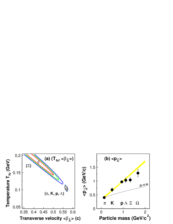
Figure 9: Mean transverse momentum $\langle P_{T}\rangle$ as a function of particle mass in central Au+Au collisions at $\sqrt{s_{NN}}=130$ GeV. Data are from STAR, yellow band from a hydrodynamically inspired fit, and the dashed line represents the expected behavior from a hydrodynamic fit at the chemical freeze-out temperature of 170 MeV at which the radial flow is still too small. Figure reprinted from [197] with permission from the American Physical Society.

Let us first review why RHIC data strongly suggests a long hydrodynamic expansion and cooling phase of the bulk matter created in nuclear collisions. We can see the clear signals of bulk collectivity in experimental data most convincingly in data on the mean transverse momentum $\langle P_{T}\rangle$ as a function of observed particle masses and in measurements of elliptic flow $v_{2}$ at RHIC. In Fig. 9 we see data on $\langle P_{T}\rangle$ for several hadron species measured in Au+Au collisions at $\sqrt{s_{NN}}=130$ GeV at RHIC, together with a band resulting from the hydrodynamically inspired fit to the $\pi$, $K$, $p$, and $\Lambda$ data [197]. The observed mass dependence clearly shows that radial flow exists and that it dominates the motion of bulk particles. Small discrepancies between data and theory exist and will be discussed in Sec. 4.

The second remarkable success of hydrodynamics is the explanation of the large elliptic flow $v_{2}$ as a function of $P_{T}$ seen at RHIC, and the characteristic dependence on mass, as shown in Fig. 26. To realize such strong elliptic flow in a leading order parton cascade model, unrealistic large cross sections are needed [198], which clearly supports a hydrodynamic interpretation. The hydrodynamical analyses also indicate that thermalization of the matter at RHIC is achieved very rapidly. Most estimates put the equilibration time between 0.6 and 1.0 fm/$c$ after the collision [4]. $v_{2}$ is a wonderful quantity to analyze with hydrodynamic models, even deviations from the expected equilibrium values can provide information on viscosities [169, 199].

Hydrodynamics assumes thermal equilibrium and very short mean free paths of particles. We know that these assumptions are broken at least at very early times and at the latest times in collisions. They might also be broken at the boundaries of the system where densities are smaller, leading to corona effects. This means that hydrodynamic calculations have to be combined with some calculations or parameterizations of the initial state, and one has to be careful about the treatment of the freeze-out, the conversion of hydro fluid cells back into particles. We can further infer from the $P_{T}$-dependence of physical observables such as elliptic flow that thermalization of particles starts to be incomplete at high $P_{T}$. At RHIC hydrodynamic models generally work very well up to $P_{T}\sim 2$ GeV/$c$. Above that threshold novel effects, like quark recombination, come into play at intermediate values of $P_{T}$. At the largest values, above 6 GeV/$c$, perturbative QCD production dominates. Of course, the hydrodynamic regime comprises about 99% of the particles produced in a typical Au+Au collision at RHIC.

3.2.2 Initial Conditions

The hydrodynamic equations of motion need initial conditions for all their dynamic variables, which are then evolved forward in time by the solutions. These initial conditions are outside of the framework of hydrodynamic models and have to be determined by other means. Physically, they are determined by the processes during the initial collision of the nuclei and the approach to equilibrium which is eventually reached at a time $\tau_{0}$. As we already discussed this equilibration time has been estimated to be rather short. However, in practice it should be a parameter since the precise equilibration mechanisms are still under debate and calculations of the initial conditions at the start of the equilibrated plasma phase have been elusive so far [200, 201].

Historically, parameterized initial conditions for entropy densities (or alternatively the energy densities) and the net baryon densities have been used [192, 202, 203, 204]. In the transverse plane these distributions are usually parameterized based on Glauber-type models of nuclear collisions. In longitudinal direction often initial distributions inspired by Bjorken’s scaling solution are used. Then few parameters remain in these initial conditions, such as the maximum values of the energy or entropy density, and net baryon density. They are usually fixed by comparison with experimental data on single particle rapidity and transverse momentum spectra.

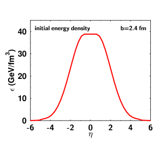
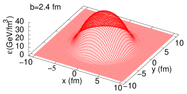
Figure 10: Initial energy density $\epsilon(\tau_{0},\eta,x,y)$ from a Glauber model in longitudinal direction (left panel) and in transverse direction (right panel)) for central Au+Au collisions. Figures taken from [192].

Let us discuss a straight forward set of energy density and net baryon density distributions that give reasonable results. We assume a factorization into a longitudinal profile $H(\eta)$ and a transverse profile $W(x,y;b)$ which are given by

$$\epsilon(x,y,\eta) = \epsilon_{\rm max}W(x,y;b)H(\eta),$$

$$n_{B}(x,y,\eta) = n_{B{\rm max}}W(x,y;b)H(\eta)\,.$$ (92)

Here the maximum values $\epsilon_{\rm max}$ and $n_{B{\rm max}}$ are parameters, $b=|\mathbf{b}|$ denotes the impact parameter of the collision, and $\eta$ is the space-time rapidity. The longitudinal distribution can be parameterized by

$$H(\eta)=\exp\left[-(|\eta|-\eta_{0})/2\sigma^{2}_{\eta}\right]\theta(|\eta|-\eta_{0})+\theta(\eta_{0}-|\eta|),$$ (93)

where parameters $\eta_{0}$ and $\sigma_{\eta}$ can also be determined by comparison with experimental data on single particle distributions. The function $W(x,y;b)$ in the transverse plane is determined by a superposition of the density of wounded nucleons — characteristic for soft particle production processes — and the density of binary collision — characteristic for hard particle production processes [202]

$$W(x,y;b)=w\frac{d^{2}N_{\rm BC}}{ds^{2}}+(1-w)\frac{d^{2}N_{\rm WN}}{ds^{2}}\,.$$ (94)

The density of wounded nucleons is given by

$$\frac{d^{2}N_{\rm WN}}{ds^{2}}=T_{A}(\mathbf{b}_{A})\left(1-e^{-T_{B}(\mathbf{b}_{B})\sigma}\right)+T_{B}(\mathbf{b}_{B})\left(1-e^{-T_{A}(\mathbf{b}_{A})\sigma}\right)$$ (95)

where $\mathbf{b}_{A}=\mathbf{s}+\mathbf{b}$, $\mathbf{b}_{B}=\mathbf{s}-\mathbf{b}$, and $\sigma\approx 42$ mbarn is the total nucleon-nucleon cross section at $\sqrt{s_{NN}}=200$ GeV [205]. $T_{A}$ is the nuclear thickness function of nucleus $A$,

$$T_{A}(\mathbf{s})=\int dz\rho_{A}(z,\mathbf{s}),$$ (96)

where the nuclear density $\rho_{A}(z,\mathbf{s})$ can e.g. be taken to be of Woods-Saxon shape

$$\rho_{A}(r)=\rho_{0}\frac{1}{1+e^{(r-R_{A})/a}}.$$ (97)

In Eq. (97) appropriate parameters $a$, $R_{A}$, and $\rho_{0}$ are 0.54 fm, 6.38 fm and 0.1688 fm^-3, respectively [205]. On the other hand, the distribution of the number of binary collisions is given by

$$\frac{d^{2}N_{\rm BC}}{ds^{2}}=\sigma T_{A}(\mathbf{b}_{A})T_{B}(\mathbf{b}_{B}).$$ (98)

The weight factor $w$ can be set to 0.6, consistent with experimental data. Figure 10 shows examples of initial longitudinal and transverse profiles. Obviously the parameters in initial conditions are truly additional uncertainties and make quantitative predictions with hydrodynamic models more difficult.

As a straight forward solution one can choose to set the initial longitudinal flow to Bjorken’s scaling solution [161], and one can set the initial transverse flow to zero. This simplest initial flow profile will serve as the basis for all further investigation here. The possibility of an initial transverse flow was discussed e.g. by Kolb and Rapp [206]. The initial flow improves the results for $P_{T}$-spectra and reduces the anisotropy. Utilizing a parameterized evolution model it has been pointed out that a Landau-type initial condition with complete longitudinal compression and vanishing initial flow is favorable for the description of the Hanbury Brown-Twiss (HBT) correlation radii [207, 208]. This suggests that HBT analyses may be a sensitive tool for the determination of the initial longitudinal flow. As we will discuss in detail in the result section, hydrodynamic calculations during the early RHIC years did show very bad agreement with experimental data, especially for the ratio of $R_{\rm out}/R_{\rm side}$, leading to the notion of an HBT puzzle [209].

Let us come back to the the apparent early thermalization times found at RHIC. Usually it is said that small initial times $\tau_{0}$ are needed to describe the elliptic flow data as elliptic flow builds up at the earliest stage of expansion when the eccentricity of the fireball is largest [165, 166]. However, we note that with suitable sets of initial conditions and freeze-out temperatures in fact a larger initial proper time is also compatible with data. Luzum and Romatschke show that three very different sets of initial and freeze-out temperature ($T_{i}$,$T_{f}$) — $(0.29,0.14)$ GeV with $\tau_{0}=2$ fm, $(0.36,0.15)$ GeV with $\tau_{0}=1$ fm, and $(0.43,0.16)$ GeV with $\tau_{0}=0.5$ fm — provide almost identical differential elliptic flow in a viscous hydrodynamic calculation [210]. This suggests that better constraints on initial conditions are indispensable to avoid wrong conclusions from comparisons of hydrodynamic calculations with experimental data.

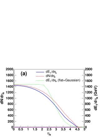
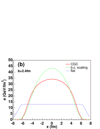
Figure 11: Initial energy density from the Color Glass Condensate in longitudinal direction (left panel) and in the transverse plane (right panel) for central Au+Au collisions at $\sqrt{s_{NN}}=200$ GeV. Figures reprinted from [211] with permission from Elsevier.

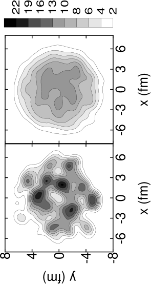
Figure 12: Examples of initial energy density profiles in the transverse plane for central Au+Au collisions given by NeXus at mid-rapidity. The energy density is plotted in units of GeV/fm³. Left panel: one random event. Right panel: average over 30 random events (similar to the smooth initial conditions often used). Figure reprinted from [216] with permission from the American Physical Society.

Other approaches for generating realistic initial conditions beyond the Glauber-based parameterizations are available. Color Glass Condensate-inspired initial conditions are becoming increasingly popular, see Fig. 11. They feature larger eccentricities than Glauber-based models which has significant implications on elliptic flow [211]. In that case additional dissipation during the early quark gluon plasma stage is needed in order to achieve agreement with experiments [211, 212]. Others models are the string rope model [213] and the pQCD + saturation model [214]. In the latter the initial time $\tau_{0}$ is given by the inverse of the saturation scale, which is set to a very short $\tau=$0.18 (0.10) fm at RHIC (LHC). More recently there is a push to implement effects of event-by-event fluctuations in initial conditions. In the NEXSPHERIO hydro model these events are created by the event generator NeXus [215]. Fig. 12 shows an example from Ref. [216]. We will discuss the implications of fluctuations in more detail later.

3.2.3 QCD and Hydrodynamics

Recent lattice QCD calculations show that the phase transition at vanishing or low chemical potential is a crossover [170, 171, 217]. However the Bag Model-based equation of state with a first-order phase transition has dominated calculations in the early RHIC years. There are several simulations of lattice QCD at high temperature and low density. However, at high net baryon density the investigation with lattice QCD becomes difficult. Because of the sign problem, we can not apply the usual Monte Carlo methods for finite density lattice QCD.

Figure 13: (a) The entropy density $s$ divided by $T^{3}$, and (b) the energy density $\epsilon$ divided by $T^{4}$ both as functions of temperature; (c) the pressure $p$, and (d) the velocity of sound squared $c_{s}^{2}=dp/d\epsilon$ both as functions of $\epsilon$. In all four panels four equations of state are shown: (i) qp = quasiparticle EoS, (ii) Q = ideal parton gas with first order phase transition, (iii) H = hadron resonance gas, and (iv) T = ansatz with crossover. Figure reprinted from [218] with permission from Elsevier.

A comprehensive study of the dependence of hydrodynamic expansion on the equation of state was carried out by Huovinen [218]. Figure 13 shows different equations of state used in Ref. [218]. Suitable parameters for the initial conditions and freeze-out temperature were chosen for each EoS so that the hydrodynamic calculation reproduces the experimental data reasonably. Huovinen found that the closest fit to the data of $v_{2}$ as a function of $P_{T}$ was obtained for a strong first-order phase transition while the results for the lattice-inspired EoS fit the data badly. Similar results were also obtained in more detailed analyses [219]. The current discrepancy between lattice results (crossover) and the hydrodynamic analysis of data (first order) is unsatisfactory. Dependences on parameters, e.g. flow in the initial conditions, and the freeze-out procedure obscure the observation of the equation of state in hydrodynamic calculations. Nevertheless, hydrodynamics offers the most direct tool to investigate the equation of state and we have to move to a comprehensive analysis including viscosities, hadronic re-interactions and an honest assessment of uncertainties from initial conditions to solve this problem in the near future.

One of the most fascinating topics in connection with the QCD phase diagram is the QCD critical point (QCP) and its possible manifestation in relativistic heavy ion collisions [220]. The possible existence of this point and its location in the QCD phase diagram have been attracting a great deal of interests. Recent studies based on effective theories show a wide range of possible locations of the critical point in the phase diagram [221]. In addition, a recent study on the curvature of the critical surface in lattice QCD shows that the existence of the QCD critical point is less than certain [222]. A solid experimental result seems the best way to settle the question of the existence of the QCP because a unanimous conclusion from lattice QCD and effective theories appears to be difficult. For quantitative tests of the existence and location of the QCP we need to run hydrodynamics with equations of state with a critical point included, and we need to identify appropriate physical observables which show clear signatures of a critical point [223, 224]. The upcoming lower energy scan at RHIC which will produce QGP at higher baryon chemical potential will provide a suitable data sample.

Relativistic viscous hydrodynamic models need more information besides the equation of state in order to run: shear and bulk viscosities, heat conductivity, and relaxation times. On the flip side one should argue that there is a unique chance at RHIC to extract quantitative values for some of these transport coefficients from data. Estimates for some transport coefficients are available from lattice QCD, finite temperature QCD perturbation theory and effective theories. For strongly coupled quark gluon plasma lattice QCD should be a reliable tool. However the determination of transport coefficients in lattice QCD with the Green-Kubo formula is not easy. Pioneering results for shear and bulk viscosities with large uncertainties have been obtained in [225, 226]. For weakly coupled QGP perturbative results have been obtained by Arnold, Moore and Yaffe [227, 228, 229]. Microscopic transport models have helped to estimate transport coefficients of a hadron gas [230, 231, 232] and a parton gas [233, 234]. The results seem to indicate that $\eta/s$ from a hadron gas is larger than the KSS bound $1/(4\pi)$ [182] which is proposed by the AdS/CFT correspondence. On the other hand, shear viscosities from radiative parton transport can be surprisingly lower than leading order perturbative results and close to the AdS/CFT bound. We have accumulated a few predictions in Fig. 34. Even though there is still little trust in quantitative numbers the preliminary conclusion is that the origin of the perfect fluid signatures at RHIC should be in the partonic phase [232].

There are also attempts to compare hydrodynamic calculations to partonic transport models. Early parton cascades with leading order dynamics [235] had suggested that large cross sections are needed to account for the elliptic flow observed at RHIC. Thermalization of the parton matter in the initial stage would be extremely slow. More recent parton cascades including radiative corrections have led to results that are compatible with large elliptic flow and rapid thermalization [236, 237, 238]. More studies comparing hydrodynamics and transport models in detail are needed as they provide necessary mutual checks.

3.2.4 The Freeze-out Process

Currently two separate freeze-out processes are believed to occur in heavy ion collisions. One is the chemical freeze-out at which the ratios of hadrons are fixed, and the other is the kinetic freeze-out at which the particles stop to interact. Chemical freeze-out temperature and chemical potentials are extracted with the statistical model on the basis of the grand-canonical formalism. Surprisingly, statistical models are in excellent agreement with experimental data for hadron ratios in a wide range of collision energy from AGS to RHIC [239]. From the values of chemical freeze-out temperatures around 170 MeV we can infer that the chemical freeze-out process takes place just after the QCD phase transition [239]. At the kinetic freeze-out temperature the mean-free path of particles has grown to be of the order of the system size and a hydrodynamic description which requires zero mean-free path is clearly no longer applicable. A first naive guess for the kinetic freeze-out temperature $T_{f}$ is the pion mass ($\sim 140$ MeV). Practically the value of the kinetic freeze-out temperature in a hydrodynamic model is determined from comparison with data for $P_{T}$-spectra.

The task at the end of a hydro calculation is the population of fluid cells of a given temperature and flow with particles. For calculations of single particle spectra, the simple assumption of a sudden freeze-out process at a certain proper time for each fluid cell is sufficient, neglecting the reverse process from particles to the hydrodynamic medium. Under this assumption the Cooper-Frye formula [240] is widely used. Here we start from a simple case [241]: Suppose that a number of particles $N(\tau)$ exists in the enclosed volume $\Omega$ that is bounded by a closed surface $S(\tau)$ at time. $N(\tau)$ is given by

$$N(\tau)=\int_{\Omega(\tau)}d^{3}r\,n(\mbox{\boldmath$r$},\tau)\,,$$ (99)

where $n(\mbox{\boldmath$r$},\tau)$ is particle number density. At time $\tau+\delta\tau$, the number of particle $N(\tau)$ has changed to

$$\frac{dN}{d\tau}=\int_{\Omega(\tau)}d^{3}r\frac{\partial n}{\partial\tau}+\frac{1}{d\tau}\int_{d\Omega}d^{3}r\,n(\mbox{\boldmath$r$},\tau),$$ (100)

where the volume has changed to $\Omega+d\Omega$. Utilizing current conservation, $\frac{\partial n}{\partial\tau}+\nabla\cdot\mbox{\boldmath$j$}$ ($j$ is the current of particles), Eq. (100) is rewritten as

$$\frac{dN}{d\tau}=-\int_{S(\tau)}d^{2}s\,\mbox{\boldmath$j$}\cdot\mbox{\boldmath$n$}+\int_{S(\tau)}d^{2}s\frac{d\zeta}{d\tau}n,$$ (101)

where $n$ is the normal vector of surface element $d^{2}s$ and $d\zeta$ is the distance between the surface of $\Omega(\tau)$ and that of $\Omega(\tau)+d\Omega$. In Eq. (101), $dN/d\tau$ is the number of particles which cross the surface $S(\tau)$ during $d\tau$. Then the total number of particles through the hypersurface $\Sigma$, which is the set of surfaces $\{S(\tau)\}$, is

$$N=\int_{\Sigma}j^{\mu}d\sigma_{\mu},$$ (102)

where $j^{0}=n$, $d\sigma_{0}=d^{3}r$, $d\mbox{\boldmath$\sigma$}=d\tau d^{2}s\,\mbox{\boldmath$n$}$. If we write

$$j^{\mu}=\frac{d^{3}P}{E}\frac{g_{h}}{(2\pi)^{3}}\frac{1}{\exp[(P_{\nu}u^{\nu}-\mu_{f})/T_{f}]\pm 1}P^{\mu}$$ (103)

for the current $j^{\mu}$ in Eq. (102), we obtain the Cooper-Frye formula [240]

$$E\frac{dN}{d^{3}P}=\sum_{h}\frac{g_{h}}{(2\pi)^{3}}\int_{\Sigma}d\sigma_{\mu}P^{\mu}\frac{1}{\exp[(P_{\nu}u^{\nu}-\mu_{f})/T_{f}]\pm 1},$$ (104)

where $g_{h}$ is a degeneracy factor of hadrons and $T_{f}$ and $\mu_{f}$ are the freeze-out temperature and chemical potential. In other words we obtain $d\sigma_{\mu}$ by estimating the normal vector on the freeze-out hypersurface $\Sigma$. Using Eq. (104), we can then calculate all particle distributions after freeze-out.

Table 2: Calculations with relativistic ideal hydrodynamical models at RHIC energies. See text for acronyms.

Ref.	IC	EoS	Hydro Exp.	hadronization & FO	observables
Kolb [165]	Glauber	1st order	2d	KF	elliptic flow
Huovinen [166]	Glauber	1st order	2d	KF	radial, elliptic flow
Kolb [202]	Glauber	1st order	2d	KF	centrality dependence of multiplicity and flow
Hirano [203]	Glauber	1st order	3d	CF and KF	flow and HBT
Teaney [204]	Glauber	1st order	2d	hadron cascade	flow, QGP signature
Nonaka [192]	Glauber	1st order	3d	hadron cascade	spectra, flow
Kolb [206]	Glauber, initial $v_{T}$	1st order	2d	CF and KF	$P_{T}$ spectra, $v_{2}$
Eskola [214]	pQCD + saturation	1st order	cylindrical symmetry	KF	low and high $P_{T}$ spectra
Hirano [211]	CGC	1st order	3d,    hydro+jet	CF and KF	$R_{AA}$, $I_{AA}$
Hirano [212]	CGC	1st order	3d	hadron cascade	$v_{2}$
Andrade [190]	NEXUS	1st order	3d	KF	$v_{2}$
Hirano [288]	CGC + fluctuation	1st order	3d	hadron cascade	$v_{2}$
Huovinen [218]	Glauber	comparison	2d	KF	hadron spectra, $v_{2}$
Socolowski [216]	NeXus	1st order	3d	CE	HBT
Hirano [268]	Glauber	1st order	3d, hydro+jet	CF and KF	hadron spectra, $v_{2}$

More realistic models have been investigated. One of them is the Continuous Emission Model (CEM) in which particles are emitted continuously from the whole expanding volume of the system at different temperatures and different times [216]. In the early days of hydrodynamics only kinetic freeze-out was implemented. Indeed, at lower collision energies such as at AGS and SPS, the differences between chemical freeze-out and kinetic freeze-out points are not large. However, at RHIC a significant difference between kinetic freeze-out temperatures from hydro-inspired models and the chemical freeze-out from the statistical model appears [242]. This phenomenon also manifests itself through the failure to get the correct absolute normalization of some $P_{T}$-spectra, e.g. the proton in hydrodynamic calculations, with only a kinetic freeze-out [243]. Hence a consistent modeling of separate freeze-out processes via modified equations of state was introduced [203, 244, 245, 246].

It turns out that some experimental data is still not understood in a satisfying way even with two separate freeze-out procedures. For example, mean transverse momentum $\langle P_{T}\rangle$ as a function of particle mass does deviate from the linear scaling law, which suggests significant final state interactions in the hadronic phase [192]. To explain these effect, and to account for the apparently large viscosities in the hadronic phase, as discussed before, hydro+cascade hybrid models were introduced. They use a hydrodynamic computation of the expansion and cooling of hot QCD bulk matter, and then couple the output consistently to a hadron-based transport model for the final-state interactions. Pioneering work on hydro+cascade hybrid models was done by Bass et al. [247] using UrQMD. Similar investigations were carried out in Refs. [204, 212]. The improvements introduced by these hybrid models are discussed in more detail in the results section.

Table 3: Calculations with relativistic viscous hydrodynamical models at RHIC energies. See text for acronyms.

Ref.	IC	EoS	Hydro Exp.	hadronization & FO	observables
Song[193]	Glauber	EoS dependence	2d, I-S	KF (direct $\pi$)	$v_{2}$
Dusling[181]	Glauber	ideal QGP gas	2d, O-G	KF, viscous corrections	$v_{2}$
Romatschke[289]	Glauber	semi-realistic EoS [248]	2d, I-S	KF	multiplicity, $v_{2}$
Luzum[210]	Glauber and CGC	semi-realistic EoS [248]	2d, conformal relativistic viscous hydro[182]	KF, viscous corrections	multiplicity, $v_{T}$, $v_{2}$
Chaudhuri[194]	Glauber	lattice +HRG EoS	2d, I-S	KF	$v_{2}$

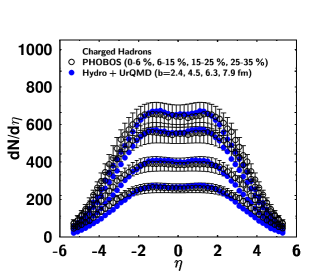
Figure 14: Centrality dependence of pseudorapidity distributions of charged particles from the hydro+UrQMD hybrid model [192] compared wit PHOBOS data for $\sqrt{s_{NN}}=200$ GeV Au+Au collisions [271]. Impact parameters in the calculation with the corresponding centrality bins in parentheses are 2.4 (0-6%), 4.5 (6-10%), 6.3 (10-15%), and 7.9 fm (25-35%). Figure taken from [192].

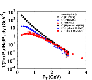
Figure 15: $P_{T}$-spectra for $\pi^{+}$, $K^{+}$ and $p$ at central $\sqrt{s_{NN}}=200$ GeV Au+Au collisions with PHENIX data [272]. The points are not renormalized. Figure taken from [192].

3.3 New Developments

Through its success at RHIC hydrodynamics has positioned itself as one of the most useful phenomenological models for heavy ion collisions. A large amount of studies working with hydrodynamics have been carried out in the RHIC era. Historically, most of them have been using ideal hydrodynamics, but obviously viscous hydrodynamics will be a major focus point for the near future, as both mathematical and numerical issues are settled. The thorough vetting of hydrodynamic models has also become a top issue. Different existing codes have to be tested against each other using identical parameters and initial conditions. One such effort is under way in the “Theory-Experiment Collaboration for Hot QCD Matter” (TECHQM) [249].

Hydrodynamic models can be easily adopted for descriptions of the entire process of heavy ion collisions that include initial collisions, thermalization, bulk dynamics, hadronization, freeze-out, final state interactions and even hard and electromagnetic probes. Such comprehensive approaches are called multi-module modeling. There are ongoing efforts to construction such models [192, 212, 250, 251]. The coupling of hydrodynamics and hadronic transport together to form a hybrid model is only the first step. Event generators for the initial state will soon become standard. It has also become necessary to conduct jet quenching studies using realistic input from hydrodynamically evolved fireballs [153].

We have compiled a list of relativistic ideal hydrodynamic models which are mentioned in this work in Tab. 2. We reference each work and quote the initial conditions, freeze-out treatment, and equation of state that have been used, and the observables that have been calculated. The acronyms KF, CF and CE stand for kinetic freeze-out, chemical freeze-out and continuous emission, respectively.

For relativistic viscous hydrodynamics, the number of phenomenological studies is much smaller. Quantitative discussions comparing to RHIC data have been carried out, but need to be weighed with caution. Many points need further study. In Tab. 3, we list the relativistic viscous hydrodynamic studies which compare results to experimental data from RHIC. Here I-S (G-O) stands for relativistic viscous hydrodynamics proposed by Israel and Stewart [173, 174, 175] (Grmela and Öttinger [176, 177, 178]). The major difference between ideal hydrodynamics (Tab. 2) and viscous hydrodynamics (Tab. 3) is that the former all agree on the set of equations to be solved, while the latter solve a variety of different second order schemes. While all of those should only exhibit small deviations from first order hydrodynamics, this strengthens the point that we have to apply due caution when analyzing RHIC data.

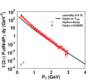
Figure 16: $P_{T}$-spectra of $\pi^{+}$ from [192]. Shown are the spectra for hydrodynamics at the switching temperature of 150 MeV, result from hydro + decay only, and hydro + full UrQMD, in central collision. Figure taken from [192].

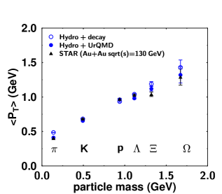
Figure 17: Mean $P_{T}$ as a function of mass. Figure taken from [192].

3.4 Hadronization and Quark Recombination

In hydrodynamic models the hadronization process from the QGP phase to the hadron phase is naturally encoded in the equation of state. As we have mentioned above hydrodynamic models generally do well for particles below $P_{T}\approx 2$ GeV/$c$ at RHIC. Between that point and the perturbative region above $\approx 6$ GeV/$c$ an intermediate $P_{T}$ region has been found. It exhibits features from both domains, without fitting exclusively in any of the two categories. E.g. we find large elliptic flow and baryon over meson ratios that are reminiscent of hydrodynamics and soft physics, and incompatible with jet quenching and fragmentation. On the other hand the elliptic flow is not large enough to follow the ideal hydrodynamic predictions, and we find dihadron correlations at intermediate $P_{T}$ that exhibit clear jet-like structures. Simple interpolations (hydro+jet models) do not explain all features, e.g. the much smaller elliptic flow of $\phi$ mesons compared to protons. In order to explain hadron production at RHIC, and in order to understand the breakdown of the pQCD or hydrodynamic approach it is crucial to understand this kinematic region at intermediate $P_{T}$.

Quark recombination or coalescence is the best candidate to explain a large amount of experimental data at intermediate $P_{T}$. Recombination models assume a universal phase space distributions of quarks at hadronization. Quarks turn into baryons, $qqq\to B$, and mesons, $q\bar{q}\to M$ described either by using instantaneous projections of quark states onto hadron states [252, 253, 254, 255, 256], or a dynamical coalescence process with finite width hadrons governed by rate equations [257]. Note that usually only the valence quarks of the hadron are taken into account although generalizations have been worked out [256].

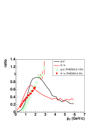
Figure 19: Ratios $N_{p}/N_{\pi^{-}}$ and $N_{K-}/N_{\pi^{-}}$ as a function of $P_{T}$ in Au + Au collisions as in Fig. 19 compared to data from PHENIX [273]. Figure reprinted from [268] with permission from the American Physical Society.

The original instantaneous projection models explicitly preserve only three components of the energy-momentum four-vector in the underlying $2\to 1$ and $3\to 1$ processes. The yield of mesons can be expressed through the convolution of the Wigner function $W_{ab}$ for parton pairs $a$, $b$ and the Wigner function $\Phi_{M}$ encoding the meson wave function

$$\frac{dN_{M}}{d^{3}P}=\int\frac{d^{3}R}{(2\pi)^{3}}\sum_{ab}\int\frac{d^{3}qd^{3}r}{(2\pi)^{3}}W_{ab}\left(\mathbf{R}+\frac{\mathbf{r}}{2},\frac{\mathbf{P}}{2}+\mathbf{q};\mathbf{R}-\frac{\mathbf{r}}{2},\frac{\mathbf{P}}{2}-\mathbf{q}\right)\Phi_{M}(\mathbf{r},\mathbf{q})\,.$$ (105)

The quark Wigner functions are usually approximated by classical phase space distributions. Hadron spectra at intermediate $P_{T}$ are described well by considering a factorization into thermal quark distributions [253]

$$W_{ab}\left(\mathbf{r}_{1},\mathbf{p}_{1};\mathbf{r}_{2},\mathbf{p}_{2}\right)=f_{a}\left(\mathbf{r}_{1},\mathbf{p}_{1}\right)f_{b}\left(\mathbf{r}_{2},\mathbf{p}_{2}\right)\,.$$ (106)

Correlations between quarks can be introduced to model correlations found between hadrons [258] without interfering with the excellent description of spectra and hadron ratios.

Dynamical models, like the resonance recombination model [257, 259, 260] solve systems of rate or Boltzmann equations for the underlying $2\to 1$ and $3\to 1$ processes. In the case of resonance recombination mesons and baryons are technically treated as resonances with widths $\Gamma_{H}$, and the inverse processes (the “decays” of mesons and baryons into quarks) are taken into account to achieve detailed balance. Resonance recombination has the advantage that is can deliver an equilibrated hadron phase from an equilibrated quark phase due to energy conservation and detailed balance. This has opened the possibility to reconcile quark recombination with hydrodynamics and equilibrium physics at low momenta [260].

At large momenta contact can be made with jet fragmentation by rewriting fragmentation functions as a process of valence quark coalescence in a suitably defined jet shower [261, 262, 263]. If $S(p)$ is the distribution of quarks in a jet before hadronization and $T(p)$ is the distribution of the underlying event (partially thermalized in heavy ion collisions) recombination will be applied to the total parton phase space $S(p)+T(p)$. For mesons this will lead to the following possible combinations: $SS$ which resembles the fragmentation process within a jet, $TS$ which is a novel “soft-hard” hadronization process, and $TT$ which corresponds to the usual picture of quark recombination. Shower distributions $S(p)$ can be fitted such that $SS$ and $SSS$ recombination fit the known fragmentation functions for the respective mesons and baryons.

The strength of the quark recombination picture is the predictive power coming from explaining all measured hadron spectra at intermediate $P_{T}$ with one parameterization of the quark phase at hadronization. It has been shown that at low momenta resonance recombination is compatible with hydrodynamics and kinetic equilibrium [260], but on the other hand, because a thermalized state does not retain memories of a previous time evolution, all phenomena in the equilibrated region should be explainable by hydrodynamics. This includes the quark number and kinetic energy scaling observed at RHIC at low momenta [260]. The possibility of including quark recombination explicitly into hydrodynamic model has been studied in [264].

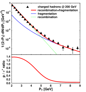
Figure 20: Top panel: inclusive $P_{T}$-spectrum of charged hadrons in central Au + Au collisions at $\sqrt{s_{NN}}=200$ GeV. Contributions from a recombination model and perturbative hadron production are shown compared to experimental data from PHENIX [274]. Bottom panel: ratio of protons to positive pions as a function of $P_{T}$ for the same Au+Au collisions. The region below 4 GeV/$c$ is dominated by recombination, the region above 6 GeV/$c$ by fragmentation of hadrons from jets. Figure taken from [252].

The quark number scaling law is a signature feature of quark recombination. For a quark phase with elliptic flow $v_{2}^{q}(P_{T})$ at the time of hadronization simple instantaneous recombination models predict

$$v_{2}^{H}(P_{T})=nv_{2}^{q}\left(\frac{P_{T}}{n}\right)$$ (107)

where $n$ is the number of valence quarks. This scaling law describes a key feature of experimental data at intermediate $P_{T}$ rather accurately. We make two comments here: (i) the general shape of $v_{2}$ at intermediate momenta suggests that in the kinematic range under consideration ($P_{T}$ between 1.5 and 5 GeV/$c$) hadrons are no longer equilibrated or at least there are large viscous corrections to hydrodynamics; (ii) at lower momentum the scaling seems to work rather with kinetic energy instead of $P_{T}$. This is a rather accidental feature of $v_{2}$ for equilibrium hydrodynamics and, as already brought up above, can not directly be attributed to quark recombination [260].

We discuss the situation from the experimental point of view further in the result section 4. More profound detours into quark recombination models are beyond the scope of this review and we refer the reader to several review articles on quark recombination for further study [265, 266, 267].

4 Interpretation of Experimental Data from RHIC

We now proceed to discuss some key experimental results from the first decade of running of the Relativistic Heavy Ion Collider. Many of those results can be understood, at least qualitatively, within the framework of perturbative QCD and hydrodynamics. We will also review some attempts to extract quantitative statements about fireball parameters and properties of quark gluon plasma. We proceed from the simplest observables, single particle yields and spectra to more intricate ones and try to take a comprehensive view that includes both bulk and hard probe particles.

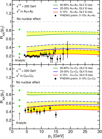
Figure 21: $R_{AA}$ for neutral pions in Au+Au and Cu+Cu collisions at top RHIC energy and for different centralities, calculated in the GLV model. Finalized PHENIX data is now available in [276]. Figure reprinted from [278] with permission from Elsevier.

4.1 Particle Multiplicities and Single Particle Spectra

Hydrodynamic models by default deliver the main qualitative features of bulk spectra measured in heavy ion collisions at RHIC: hadrons at low transverse momentum $P_{T}$ are thermalized and exhibit a relativistic outward collective flow. Nevertheless it is a challenge to quantitatively describe details, like the subtle differences seen between hadron species. If we want to describe bulk observables with hydrodynamics or hybrid models based on hydrodynamics the first goal is the determination of realistic initial conditions. Even if some theoretical modeling of the initial state is available, there are usually a few parameters that are fitted to single particle $P_{T}$-spectra and rapidity distributions in central collisions.

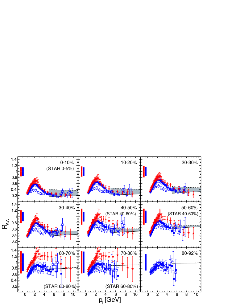
Figure 22: $R_{AA}$ for several centrality bins for Au+Au collisions at top RHIC energy. Calculations using ASW energy loss with reweighted (dashed) and non-reweighted quenching weights (solid lines) are compared to data from PHENIX for charged hadrons (closed squares) and neutral pions (open squares) [2, 279], and from STAR for charge hadrons [3]. Figure reprinted from [124] with kind permission from Springer Science + Business Media.

In Figs. 15 and 15 we show single particle spectra from a hybrid model of (3+1)-dimensional ideal, relativistic hydrodynamics and UrQMD [192]. In this model final state interactions at the end of the fireball life time are taken into account by connecting the hydrodynamic phase to the hadron-based event generator. For the determination of initial conditions, this hybrid model works the same way as pure hydrodynamics. Practically, the parameters to be determined are the maximum values of energy density and baryon number density which are fixed from comparison with experimental data of pseudorapidity distributions and $P_{T}$-spectra in central collisions. The centrality dependence of spectra is then settled and reproduces the data well as shown in Fig. 15.

Figure 15 compares the $P_{T}$-spectra for $\pi^{+}$, $K$ and $p$ in central Au + Au collisions. Because the hybrid model correctly treats chemical and kinetic freeze-out processes, taking into account the different cross sections of hadrons, the absolute value of the proton spectra shows good agreement with the experimental data. This is one of the improvements that hybrid models with hadronic transport offer over pure hydrodynamic model with only one (thermal) freeze-out process. Such pure hydro calculations usually fail to explain proton spectra. Clearly, taking into account the correct freeze-out for each particle species separately is important and hybrid models with hadronic transport deliver that.

Let us now investigate the detailed effect of resonance decays and hadronic rescattering on the shape of the momentum spectra. Figure 17 compares the $P_{T}$-spectrum for $\pi^{+}$ from hydrodynamics only, i.e. at the switching temperature $T_{\rm sw}=150$ MeV of the hybrid model (solid line), to the spectrum after resonance decays have been taken into account in addition (open symbols). We also show the result if the full UrQMD transport is run on the hydro result (solid circles). The difference between the solid line and open symbols directly quantifies the effect of resonance decays on the spectrum. They obviously increase the yield of pions, most dominantly in the low momentum region $P_{T}<1$ GeV/$c$. Furthermore, the difference between open and solid symbols quantifies the effect of hadronic rescattering. Pions with $P_{T}>1$ GeV lose momentum resulting in a steeper slope. In other words hadronic re-interactions cool the spectra. However, they do it selectively with the appropriate cooling rates for different hadron species.

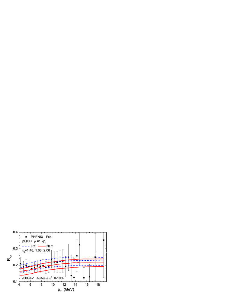
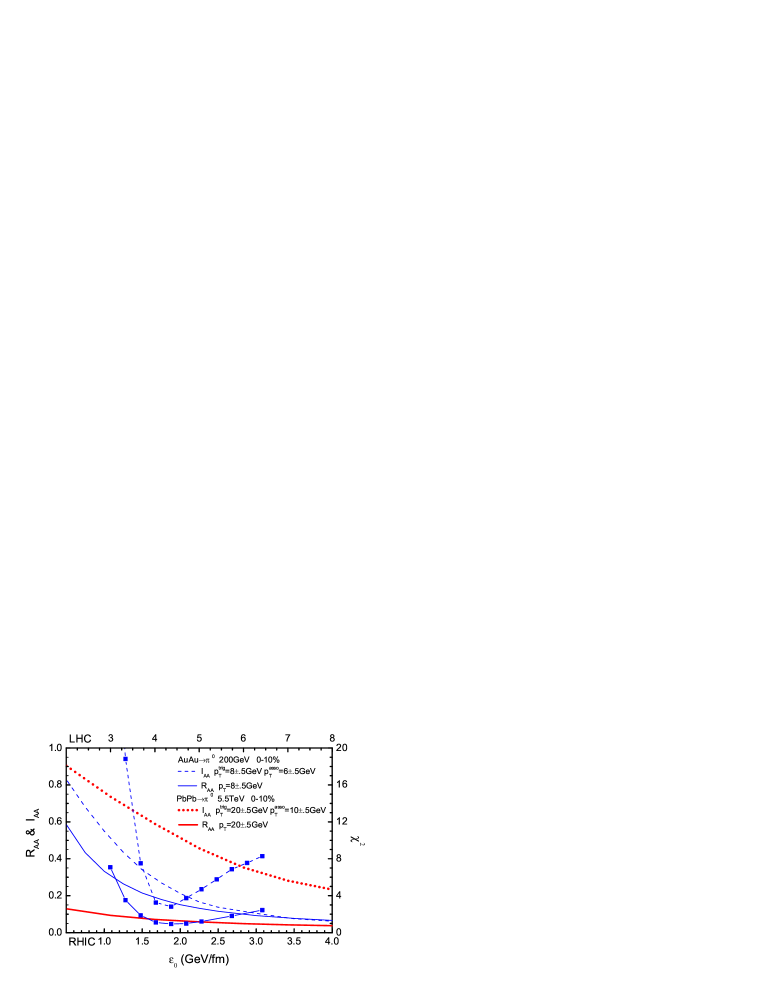
Figure 23: Left panel: $R_{AA}$ of neutral pions for central Au+Au collisions at top RHIC energies using LO and NLO accuracy hard processes and medium-modified fragmentation functions from the Higher Twist formalism compared to data from PHENIX. Finalized PHENIX data available in [276]. Right panel: $\chi^{2}$-fit of $\epsilon_{0}$ to RHIC data on $R_{AA}$ and $I_{AA}$ yielding a consistent value for both observables. Figures reprinted from [280] with permission from the American Physical Society.

To strengthen this point we show the mean transverse momentum $\langle P_{T}\rangle$ as a function of hadron mass from [192] in Fig. 17. As before we compare results at the switching temperature $T_{\rm sw}=150$ MeV, corrected for hadronic decays (open symbols) to the results from hydro plus full UrQMD (solid symbols). In the former case $\langle P_{T}\rangle$ follows a straight line, as expected from a hydrodynamic expansion. It is a natural consequence of collective flow. If hadronic rescattering is taken into account $\langle P_{T}\rangle$ does no longer follow the straight line. The average momentum of pions is actually reduced by hadronic rescattering (they act as a heat bath in the collective expansion), whereas protons pick up additional transverse momentum in the hadronic phase. Data by the STAR Collaboration is shown as well (solid triangles). The proper treatment of hadronic final state interactions significantly improves the agreement of the calculation with the data.

Generally, $P_{T}$-spectra from hydrodynamic calculations show good agreement with experimental data up to $P_{T}\sim 2$ GeV/$c$. For larger $P_{T}$ discrepancies between hydrodynamic results and experimental data appear, which suggest the approximate limits of applicability for hydrodynamics. We can see these discrepancies between hydrodynamic results and experimental data in spectra in Fig. 19 and in elliptic flow in Fig. 28 (which we discuss in more detail later). The general features of extended spectra can usually be described in hydro plus jet models, as e.g. shown in Ref. [268].

Figure 19 shows $P_{T}$-spectra for $\pi^{-}$, $K^{-}$ and $p$ in Au + Au collisions at $\sqrt{s_{NN}}=200$ GeV. The dotted lines indicate ideal hydrodynamics. These spectra exhibit a Boltzmann-like shape ($\sim\exp(-E/T)$) which is locally boosted by a radial flow velocity $\langle u^{\mu}\rangle$ through $E\to p_{\mu}u^{\mu}$. This is the gross feature of all $P_{T}$-spectra in hydrodynamic models and comparison with data suggests that thermalization is reached. The figure also shows the contributions from hard (pQCD) hadron production (dash-dotted lines), whose spectra exhibit power-law behavior. Because of the exponential suppression of the bulk perturbative hadron production dominates at large enough $P_{T}$. The sum of both hydro and perturbative (“jet”) contributions describes the data quite well. The value of $P_{T}$ where the transition from the soft to the hard component takes place depends on particle species. In the case of pions it happens between $P_{T}\sim 1$ and $P_{T}\sim 2$ GeV/$c$ in this particular calculation. For protons the transition happens gradually in the range $2\leq P_{T}\leq 5$ GeV/$c$, but certainly at higher momentum than for pions. The crossing point is determined by two facts: one is radial flow which pushes the soft components toward high $P_{T}$. The other is the jet quenching mechanism which suppresses contributions from jets. However, the simple hydro+jet model does not explain some striking features of the systematics of different particle species.

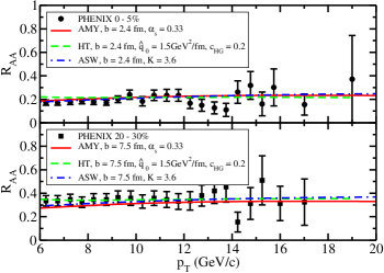
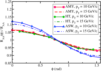
Figure 24: Left panels: $R_{AA}$ as function of $P_{T}$ for central (top) and mid-central (bottom) collisions calculated from the ASW, Higher Twist and AMY energy loss models. The single parameter in each model has been fitted to describe the data by PHENIX (finalized data available in [276]). Right panel: $R_{AA}$ as function of azimuthal angle $\phi$ normalized by the $\phi$-integrated value for two different values of $P_{T}$. Again all three energy loss models are shown. Figures taken from [153].

The differences in the transition points for different particles come from the different (mass dependent) effects of radial flow, and from the different yields of these particles in the fragmentation process (which disfavors heavier mesons and baryons). The effects of different crossing points are most clearly seen in hadron ratios as a function of $P_{T}$. In Fig. 19 we show the hadron ratios $p/\pi^{-}$ and $K^{-}/\pi^{-}$ as a function of $P_{T}$ from the hydro+ jet model advocated in [268]. A crucial point in this figure is the fact that the ratio of $p/\pi^{-}$ is as large as unity at $P_{T}\approx 3$ GeV/$c$, which can not be understood from pQCD. This anomalously large yield of protons at intermediate $P_{T}$ was the first indication of the so-called baryon puzzle.

It was the baryon puzzle that gave birth to quark recombination models in the RHIC era. Most of the experimental evidence for recombination comes from elliptic flow measurements, but the large baryon/meson ratios were essential to highlight the necessity for a mechanism that is able to push the region of soft physics farther out for baryons than for mesons. One crucial event was the advent of first data on the $\phi$ meson. In a hydro+jet model $\phi$s essentially behave like protons, because of their mass, while in data they exhibit the universal behavior of other mesons (pions, kaons) at intermediate $P_{T}$ [253, 269, 270].

Figure 20 shows the $P_{T}$-spectrum of charged particles and the $p/\pi^{+}$ ratio as a function of $P_{T}$ from the model advocated in [252] which includes quark recombination and hadrons from pQCD (“fragmentation”). The proper hydrodynamic region below 2 GeV/$c$ has been omitted. From comparison with experimental data from STAR one can conclude that the region below 4 GeV/$c$ is actually dominated by quark recombination while the pure pQCD region free of soft or bulk hadron production only starts beyond 6 GeV/$c$. Similar conclusions have been reached in other recombination + jet models. We will find even stronger evidence when we discuss elliptic flow in the next subsection, where recombination shows clearly visible and experimentally tested differences compared with both hydrodynamics and perturbative hadron production.

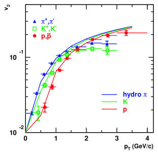
Figure 25: $v_{2}(P_{T})$ for pions, kaons and protons produced in minimum-bias collisions at RHIC from an ideal hydro calculation by Huovinen et al. [166] compared to data from PHENIX [281]. Figure reprinted from [281] with permission from Elsevier.

Figure 26: $v_{2}$ as a function of pseudorapidity $\eta$ for charged hadrons in Au+Au collisions at $\sqrt{s_{NN}}=130$ GeV. The solid and dashed lines correspond to the hydrodynamic calculations with partial chemical equilibrium (PCE) and full chemical equilibrium (CE) respectively. Data is taken from STAR [282] and PHOBOS [285]. Figure reprinted from [203] with permission from the American Physical Society.

Beyond 6 GeV/$c$ in transverse momentum hadron spectra are dominated by perturbative production that includes energy loss through final state interactions with the medium and fragmentation. Since the interesting observable is the suppression with respect to high-$P_{T}$ jets and hadrons in the vacuum the best way to analyze the data is by considering the ratio

$$R_{AA}=\frac{dN^{(AA)}/dP_{T}}{\langle N_{\mathrm{coll}}\rangle dN^{(pp)}/dP_{T}}$$ (108)

of yields in A+A vs $p+p$ collisions. This nuclear modification factor is similar to what we had defined in Eq. (38) for $d+$A collisions. $\langle N_{\mathrm{coll}}\rangle$ is the average number of binary nucleon-nucleon collisions that we expect for a given centrality bin. It is usually determined from Glauber-type model calculations. An incoherent superposition of nucleon-nucleon collisions would lead to $R_{AA}=1$ modulo isospin effects. We have already discussed in Sec. 2.2.4 how initial state nuclear effects lead to modest deviations from unity.

As had been predicted, first RHIC data at high $P_{T}$ revealed a huge suppression of hadrons [2, 3, 275, 276, 277]. This strong jet quenching is one of the pillars on which a qualitative argument for the creation of quark gluon plasma at RHIC energies rests. Fig. 21 shows calculations by Vitev within the GLV model for the $R_{AA}$ of neutral pions in Au+Au and Cu+Cu at RHIC energies of $\sqrt{s_{NN}}=200$ GeV for different centralities [278]. The calculation also takes into account nuclear effects in the initial state. The quenching is as large as a factor 5 in central Au+Au collisions as indicated by the data from PHENIX. Vitev connects the quenching strength $\hat{q}$ to a local gluon density $dN_{g}/dy$ in the medium and he finds $dN_{g}/dy\approx 800-1175$ for central Au+Au collisions.

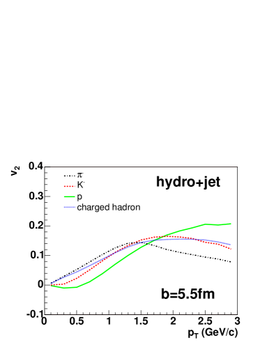
Figure 27: Elliptic flow $v_{2}(P_{T})$ for $\pi^{-}$, $K^{-}$, and $p$ in Au+Au collisions at $\sqrt{s_{NN}}=200$ GeV at impact parameter $b=5.5$ fm from the hydro+jet model [268]. Figure reprinted from [268] with permission from the American Physical Society.

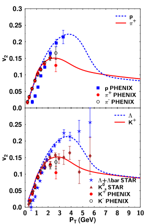
Figure 28: Upper panel: $v_{2}$ for $p$ and $\pi^{+}$ from the recombination plus fragmentation model in [252]. Lower panel: $v_{2}$ for $K^{+}$ and $\Lambda+\bar{\Lambda}$ from the same model. Data shown is from PHENIX [283] and STAR [284]. Figure taken from [252].

Figure 22 shows a systematic study of the centrality dependence of the $R_{AA}$ of charged hadrons in Au+Au collisions carried out by Dainese, Loizides and Paic using an implementation of the ASW energy loss model [124]. They model the centrality dependence by scaling not only the production of jets but also the local $\hat{q}$ by the density of binary nucleon-nucleon collisions, $\hat{q}(\mathbf{x})=kn_{\mathrm{coll}}$. This is different from other approaches that usually scale soft particle densities in the transverse plane by the density of nucleon participants $n_{\mathrm{part}}$. The centrality dependence of the data from PHENIX and STAR is reproduced well by just one adjustable parameter, the normalization $k$. So far, no conclusive picture has emerged which scaling of $\hat{q}$ is favored by data. The fit to data is aided by the large theoretical uncertainty that comes from the difference between the reweighted and non-reweighted versions of the ASW quenching weights that have been discussed earlier. Those two results define the grey bands in Fig. 22. The average quenching found by the authors within the ASW formalism is $\hat{q}\approx 15$ GeV²/fm. This value, like others obtained with the ASW model, are rather large compared to those from alternative energy loss calculations as we will see below.

Zhang et al. have presented one of the first studies of jet quenching using next-to-leading order hard processes [280]. The left panel of Fig. 23 compares their results for the $R_{AA}$ of $\pi^{0}$ in central Au+Au collisions at LO and NLO accuracy with data from PHENIX. They use medium-modified fragmentation functions inspired by the Higher Twist formalism that are rescaled by the average energy loss of a parton, and then use these instead of NLO vacuum fragmentation functions in a next-to-leading order code for hadron production. They parameterize the energy loss through an integral over a transverse profile of an expanding fireball along the path of the parton times a normalization parameter $\epsilon_{0}$ that characterizes the stopping power parameter of the medium. The left panel of Fig. 23 shows their result for three different values of $\epsilon$ that define an approximate uncertainty band. Both the LO and NLO calculations can describe the data if $\epsilon_{0}$ is a fit parameter. If $\epsilon_{0}$ is kept fixed the NLO calculation shows stronger quenching due to the larger ratio of gluon to quark jets which couple more strongly to the medium. The right panel of Fig. 23 shows a $\chi^{2}$-fit of $\epsilon_{0}$ to $R_{AA}$ between 4 and 20 GeV/$c$ and to $I_{AA}$ (discussed below), yielding consistent values in a range $\epsilon_{0}=1.6\ldots 2.1$ GeV/$c$ [280].

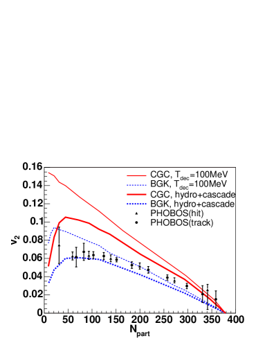
Figure 29: $P_{T}$-integrated elliptic flow for charged hadrons at midrapidity ($|\eta|<1$) from Au + Au collisions at RHIC top energy as a function of the number of participating nucleons $N_{\rm part}$. Thin lines show the predictions from ideal fluid dynamics only with a freeze-out temperature $T_{\rm dec}=100$ MeV while thick lines indicate the results from the hydro+JAM hybrid model. For both models two different initial conditions, CGC and BGK, are used. Figure reprinted from [212] with permission from Elsevier.

Fig. 24 shows results from a comparative study by Bass et al. Jets are propagated through a medium described by hydrodynamics, using three different schemes for energy loss: ASW, Higher Twist, and AMY [153]. The left panels show $R_{AA}$ as a function of $P_{T}$ for two different centrality bins. They serve as proof that both the $P_{T}$-dependence and the centrality dependence of $R_{AA}$ can be described by all three models. Every model has one free parameter that has been fitted: the strong coupling $\alpha_{S}$ for AMY, $\langle\hat{q}\rangle$ or derived parameters for the HT and ASW formalisms. In this particular case a normalization factor $K=\hat{q}/(2\epsilon^{3/4})$ as explained in Eq. (80) was fitted for ASW, where $\epsilon$ is the local energy density.

This study confirms the surprisingly large $\hat{q}$ found in the ASW model compared to other approaches. For the case that the quenching strength scales with $\epsilon^{3/4}$ the initial values found for a quark at the center of the fireball in central collision are [153]

$$\hat{q}=18.5\>\text{GeV}^{2}/\text{fm for ASW}\,,\qquad\hat{q}=4.5\>\text{GeV}^{2}/\text{fm for HT}$$ (109)

and for the case that the quenching strength scales like the temperature $T$ it is found that

$$\hat{q}=10\>\text{GeV}^{2}/\text{fm for ASW}\,,\qquad\hat{q}=2.3\>\text{GeV}^{2}/\text{fm for HT}\,,\qquad\hat{q}=4.1\>\text{GeV}^{2}/\text{fm for AMY}\,.$$ (110)

Recall that the rates in AMY are calculated self-consistently as functions of the local temperature so there is only one choice to model the space and time dependence.

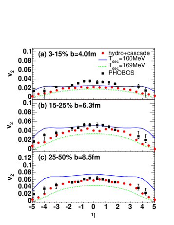
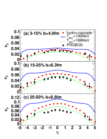
Figure 30: Left panel: The pseudorapidity dependence of $v_{2}$ for charged hadrons in (a) central (3-15%), (b) semi-central (15-25%), and (c) peripheral (25-50%) Au + Au collisions at $\sqrt{s_{NN}}=200$ GeV. The corresponding impact parameters are $b=4.0$, 6.3, and 8.5 fm resp. The hydrodynamic evolution is initialized with modified BGK initial conditions. The lines show the predictions from ideal fluid dynamics only for freeze-out temperatures of $T_{\rm dec}=100$ MeV (solid blue) and $T_{\rm dec}=169$ MeV (dashed green). Red circles show the corresponding results from the hydro+JAM hybrid model. Right panel: Same as left panel, except for using CGC instead of BGK initial conditions. Figures reprinted from [212] with permission from Elsevier.

This comparison is unique and very valuable since the same initial hard cross sections and the same maps for the fireball, from (3+1)-dimensional ideal hydrodynamics were used. Any differences in the extracted values of $\hat{q}$ must be due to differences between the calculations themselves, not due to differences in implementation. One of the conclusions is that our current knowledge applied to $R_{AA}$ leaves a rather large uncertainty in the determination of $\hat{q}$.

The right panel of Fig. 24 shows $R_{AA}$ as a function of the angle $\phi$ with respect to the reaction plane normalized by the average $R_{AA}$. Due to the large values of $\hat{q}$ the ASW formalism is more strongly dominated by surface emission than the other models. This also leads to a stronger angular modulation for non-spherical fireballs.

4.2 Azimuthal Anisotropies and Elliptic Flow

Anisotropies in the azimuthal angle $\phi$, especially elliptic flow, contain detailed information on the hot and dense QCD bulk matter created at RHIC. We will use the notion of elliptic flow for the second harmonic

$$v_{2}(P_{T})=\frac{\int d\phi\cos 2\phi\,dN/d\phi dP_{T}}{\int d\phi\,dN/d\phi dP_{T}}$$ (111)

for any value of $P_{T}$, even if the asymmetry is not produced through hydrodynamic flow. Large elliptic flow of the bulk matter produced at RHIC had been observed early on and has led to the claim of perfect fluidity of the quark gluon plasma just above $T_{c}$ [9]. With the advent of viscous relativistic hydro codes the interest has shifted toward the goal of quantifying the dissipative transport coefficients, in particular the shear viscosity $\eta$.

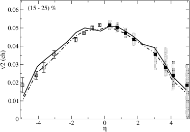
Figure 31: Comparison between true elliptic flow (solid line) and a suggested method to compute reconstructed elliptic flow from data $v^{\rm Rec}_{2}$ (dash-dotted line). Squares represent PHOBOS data for mid-central collisions [285, 286, 287]. See Ref. [190] for detail. Figure reprinted from [190] with permission from the American Physical Society.

In the hydrodynamic regime the asymmetry in the pressure gradient in and out of the reaction plane for finite impact parameters drives a larger acceleration in-plane than out-of-plane. Figure 26 shows the elliptic flow $v_{2}$ as a function of $P_{T}$ for $\pi$, $K$ and $p$ from an early calculation using ideal hydrodynamics by Huovinen et al. [166]. The calculations show remarkable agreement with experimental data. We can observe a clear mass ordering: the $v_{2}$ for pions is larger than that of kaons which in turn is larger that that of protons. The effect is most pronounced at low $P_{T}$. This is a natural phenomenon in hydrodynamics and comes from the interplay of radial flow in and out of the reaction plane. The effects of flow are more pronounced for more massive particles due to their smaller thermal velocities at a given temperature, which translates into smaller asymmetries. As for spectra the good agreement between hydrodynamic models and experimental data is restricted to low $P_{T}$ as effects of insufficient thermalization kick in at higher momenta. Despite the pioneering character of this calculation it is at present no longer regarded as being very realistic due to the following issues: (i) the lack of proper treatment of chemical vs thermal freeze-out, (ii) the fact that it assumes boost-invariance and ignores the dynamics in longitudinal direction, (iii) the absence of final state interactions, (iv) the absence of dissipative corrections. As we had pointed out earlier hydrodynamic models that do not take into account the difference of chemical and kinetic freeze-outs can not explain the absolute values of proton spectra correctly. However this calculation gives us the guidelines for the necessary improvements that have been implemented since then.

Figure 26 shows elliptic flow at RHIC as a function of pseudorapidity $\eta$. This calculation is carried out with a (3+1)-dimensional ideal hydro model with two freeze-out processes (labeled PCE = partial chemical equilibrium) [203]. These features improve the $P_{T}$-spectra of protons and give reasonable results for $v_{2}(P_{T})$ for $\pi$, $K$ and $p$ at midrapidity. However the authors of this study find that they can not explain the data from RHIC away from midrapidity. Besides generally overestimating transverse flow, there are humps in forward and backward rapidity which do not feature in the experiment data [282, 285]. It should be noted that the rapidity spectra are described well after two adjustable parameters in the initial conditions in longitudinal direction had been fixed. This result might indicate that thermalization is reached only very close to midrapidity.

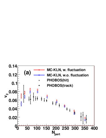
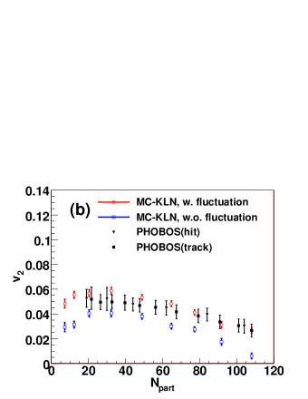
Figure 32: Left panel (a): Centrality dependences of $v_{2}$ for charged particles at midrapidity in Au+Au collisions at $\sqrt{s_{NN}}=200$ GeV with CGC initial conditions. Open circles (squares) are results with (without) eccentricity fluctuations. Right panel (b): The same for Cu+Cu collisions. Figures reprinted from [288] with permission from the American Physical Society.

As in the case of spectra one can also infer from comparison of elliptic flow with data that hydrodynamic models work only at $P_{T}<2$ GeV/$c$, see Fig. 26. Naturally we expect a transition to a region that is dominated by perturbative production, with a recombination region in between. Note that the mechanism of $v_{2}$ generation is different for hard probes. An azimuthal asymmetry develops simply because of the different amount of material jets have to go through in- and out-of-plane, with smaller opacity in-plane. Fig. 28 shows $v_{2}$ as a function of $P_{T}$ for $\pi^{-}$, $K^{-}$, $p$ and charged hadrons for the hydro + jet model in [268]. In experimental data we observe that the shape of the $P_{T}$-dependence of $v_{2}$ changes from that of a pure hydro model by bending over at larger $P_{T}$, saturating for a while at intermediate $P_{T}$, and then dipping down at even larger values of $P_{T}$. The transition points, as for spectra, depend on particle species. In addition, the saturation levels at intermediate $P_{T}$ shows a peculiar universality with baryons and mesons lining up at two different values of $v_{2}$ which scale like 3:2 [5, 6].

Hydro + jet models get some of these basic features, but usually can not explain the systematics of transition points and the universal baryons vs meson saturation levels. This is a strong argument for the presence of quark recombination at intermediate $P_{T}$. Figure 28 shows $v_{2}$ as a function of $P_{T}$ for identified particles from the recombination plus fragmentation model advocated in Ref. [252] together with early experimental data. Recombination models naturally deliver the universal behavior within the baryon and meson groups and indeed predict the valence quark number scaling of $v_{2}$ as discussed earlier in this review. The data clearly support this stunning feature and have supported the claim that traces of collectivity at the parton level can be seen [252]. At higher $P_{T}$ perturbative hadron production takes over. It is generally expected that $v_{2}$ in the perturbative domain does not depend too much on hadron species, but reliable data above 6 GeV/$c$ is scarce. Large differences between hadrons could be a sign of hadron- instead of parton-based jet quenching, or they could indicate rapid changes in jet chemistry inside a quark gluon plasma [140]. We discuss more theoretical results for $v_{2}$ at high $P_{T}$ below. Figure 28 shows general agreement of the calculations with data except for the small $P_{T}$-region where the mass splitting is not resolved since no genuine hydrodynamics phase with correct hadron masses was used.

While recombination models lend a helpful hand to hydrodynamics to extend the bulk properties to larger $P_{T}$, hadronic transport is able to fix our failing understanding of the pseudorapidity dependence discussed earlier, and of the centrality scaling of elliptic flow [192, 212]. In Fig. 29 we show the $P_{T}$-integrated elliptic flow for charged hadrons at midrapidity as a function of the number of participating nucleons $N_{\rm part}$. The plot compares results obtained with an ideal (3+1)-dimensional hydrodynamic model with and without the hadronic cascade model JAM attached as an afterburner from Hirano et al. [212]. In this study the authors also compare two different initial conditions for their hybrid model: a Glauber model (BGK) and Color Glass Condensate-based model (CGC). We refer the reader to Ref. [212] for more details. We observe that the hybrid hydro+JAM model with Glauber initial conditions gives the best description of the centrality dependence of elliptic flow. The hydro+JAM model with CGC initial conditions which is generally considered more realistic is consistent with experimental data only at large $N_{\rm part}$.

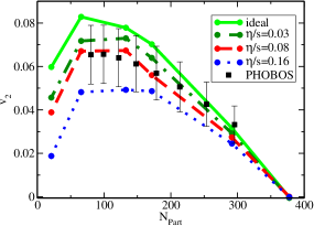
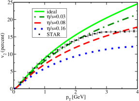
Figure 33: Left panel: Integrated $v_{2}$ as a function of $N_{\rm part}$ for charged particles in Au+Au collisions at $\sqrt{s_{NN}}=200$ GeV, compared to viscous hydrodynamics with shear viscosity for various viscosity-to-entropy ratios $\eta/s$ and compared to data from PHOBOS [290]. Right panel: $v_{2}$ as a function of $P_{T}$ for the same system compared to data from STAR [291]. Figures reprinted from [289] with permission from the American Physical Society.

The pseudorapidity dependence of $v_{2}$ for charged hadrons in central, semi-central and peripheral Au+Au collisions at $\sqrt{s_{NN}}=200$ GeV is shown in Fig. 30. By comparing results from pure ideal hydrodynamics at decoupling temperatures of $T_{\rm dec}=100$ MeV and $T_{\rm dec}=169$ MeV respectively, we see that the bumps at forward and backward rapidities that were already observed in the previous study [203] are larger if the hadronic matter is allowed to evolve without dissipation. On the other hand, $v_{2}(\eta)$ from the hybrid hydro plus hadronic cascade model does not allow these structures to build up in $v_{2}(\eta)$. We can conclude from all of these hybrid studies with hadronic cascades that effects of shear viscosity and dissipation in the hadronic phase, and proper final state interactions are not negligible. We also note that once more the initial conditions based on the Glauber model have the upper hand over CGC initial conditions in comparison with data. Color glass initial conditions would require additional dissipation during the QGP phase. However, even this much improved investigation did not take into account the effect of event-by-event fluctuations of the geometric shape of the density of the initial condition which affects the elliptic flow.

The importance of including event-by-event fluctuations was discussed systematically by Andrade et al. using the hydrodynamic code NEXSPHERIO [190] which includes a Monte-Carlo generator for initial conditions. They show that the assumption of symmetry of the particle distribution in relation to the reaction plane leads to disagreement between the true and reconstructed elliptic flows and emphasize that it is important to have a precise experimental determination of elliptic flow. Their calculated $v_{2}$ as a function of pseudorapidity shows very nice agreement with experimental data as shown in Fig. 31. However, they did not connect their hydrodynamic model to a transport code for the hadronic phase.

The effect of eccentricity fluctuations on the elliptic flow at midrapidity in Au +Au and Cu + Cu collisions was recently also investigated in Ref. [288]. Those authors include the effect of initial eccentricity fluctuations originating from the nucleon position inside the colliding nuclei both for the Glauber model and CGC initial conditions. The effect of eccentricity fluctuations is not very large in semi-central Au + Au collisions and it does not shift the values of $v_{2}$ closer to experimental data in that region. On the other hand, it enhances $v_{2}$ in Cu + Cu collisions where fluctuations are more important because of the smaller system size. As a result $v_{2}(\eta)$ from CGC initial conditions with fluctuations can describe the experimental data quite well.

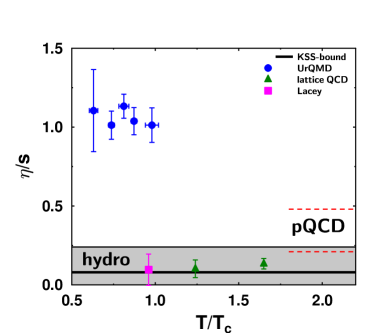
Figure 34: Estimated band of $\eta/s$ form current viscous hydrodynamics models in Tab. 3 and from several theoretical estimates discussed in the text.

Finally we show results for elliptic flow from one of the recently developed (2+1)-dimensional relativistic viscous hydrodynamic codes. Since both the formulation and the implementation of relativistic, second order viscous hydrodynamics is non-trivial, qualitative comparison with experimental data is just starting. Figure 33 shows results for $v_{2}$ of charged particles in Au+Au collisions obtained by Romatschke and Romatschke [289] together with experimental data from STAR and PHOBOS. This study finds that both integrated $v_{2}$ as a function of centrality, and differential $v_{2}$ as a function of $P_{T}$ need very small values of $\eta/s$, $0.03\ldots 0.08$, partially violating the conjectured KSS bound. It is too early to reach conclusive results in light of the many small improvements that ideal hydrodynamics needed to implement over a decade to become a reliable tool. E.g. the study mentioned here considers only one type of initial condition (Glauber) and it does not implement final state interactions [289]. Nevertheless, the first efforts have jump started the era of qualitative studies using dissipative hydrodynamics [179, 292].

In Fig. 34 we show a band for favored values of the shear viscosity over entropy ratio $\eta/s$ which is extracted from the recent viscous hydrodynamic models listed in Tab. 3. We also show results from lattice QCD [226], UrQMD [232], pQCD (Fig. 10 in Ref. [179]) and phenomenological analyses [293] for reference. This $\eta/s$ band from viscous hydrodynamics should not be considered as a conclusive result, but it highlights an interesting preliminary finding: The $\eta/s$ extracted from comparison of viscous hydrodynamics with RHIC data is generally in the vicinity of the KSS bound. From the comparison with UrQMD and lattice QCD, we would conclude that those small values of $\eta/s$ must come from the QGP phase. These facts support the hypothesis of a sQGP at RHIC. In these viscous hydrodynamic calculations the temperature dependence of viscosities is usually not taken into account, as shown in Fig. 34. The temperature dependence of transport coefficients may be not very significant in the QGP phase at RHIC. However the shear viscosity of the hadron phase seems to be much larger than that of the QGP phase which suggests that it is necessary to take this difference into account when discussing phenomena related to the QCD phase transition [168].

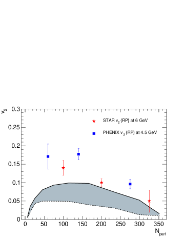
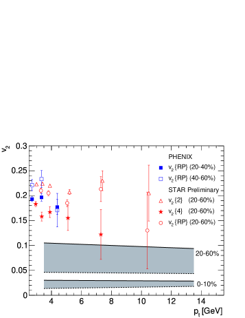
Figure 35: Left panel: $v_{2}$ as a function of $N_{\mathrm{part}}$. Right panel: $v_{2}$ as a function of $P_{T}$ for two different centrality bins. As in Fig. 22 dashed lines refer to reweighted and solid lines to non-reweighted ASW quenching weights. STAR and PHENIX data from references [283, 294, 295]. Figures reprinted from [124] with kind permission from Springer Science + Business Media.

Let us come back to the problem of azimuthal anisotropy at large $P_{T}$. We have already discussed the basic mechanism how perturbative hadron production with final state interaction in a medium can lead to positive $v_{2}$. We want to close this subsection by showing the $v_{2}$ obtained in the study by Dainese, Loizides and Paic, using the ASW formalism, that we already discussed for their results on $R_{AA}$ in the previous subsection [124]. Fig. 35 shows $v_{2}$ as a function of centrality (left panel) and as a function of $P_{T}$ (right panel) with data from STAR and PHENIX. We notice that the asymmetry from the difference in opacity in- and out-of-plane can be sizable, but the calculation still underestimates most of the data. The large $v_{2}$ measured by experiments at large $P_{T}$ has long been puzzling, but the experimental data also exhibits large error bars. Note that $\hat{q}$ was fixed in order to describe $R_{AA}$ which leaves no free parameter in this study.

We want to remind the reader of the right panel in Fig. 24. In that study $R_{AA}$ was investigated as a function of the azimuthal angle $\phi$ with respect to the reaction plane, not just integrated over $\phi$. In principle $R_{AA}(\phi,P_{T})$ has more differential information than either $v_{2}$ or integrated $R_{AA}$. We recall that the ASW formalism exhibited the strongest angular modulation and has therefore the largest $v_{2}$ in that comparative study.

Figure 36: HBT radii for negative pions in (from the top) side, out, and long directions and the ratio $R_{\rm out}/R_{\rm side}$ (bottom) as function of pair momentum $K_{T}$. Solid and dashed lines correspond to hydro calculations using partial chemical equilibrium (PCE) and full chemical equilibrium (CE) resp. STAR and PHENIX data from Refs. [297, 298] Figure reprinted from [203] with permission from the American Physical Society.

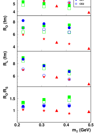
Figure 37: HBT radii and the ratio $R_{\rm out}/R_{\rm side}$ for four different scenarios for initial condition and freeze-out, see text for details. Data for pions from STAR and PHENIX are shown [297, 298]. Figure reprinted from [216] with permission from the American Physical Society.

4.3 Two-Particle Correlations

Before RHIC started up two-pion Hanbury Brown-Twiss (HBT) interferometry was believed to give us a clear signature of the QCD phase transition. We expected that an enhancement of the ratio of the inverse width of the pion correlation function in out-direction to that in side-direction, which results from a prolonged life time of the fire ball with a phase transition, could be observed at RHIC [296]. However what we find in experimental data from RHIC are HBT radii that are almost the same as those measured at SPS [281]. Furthermore, most present hydrodynamic models can not describe the measured HBT radii correctly although they fit both spectra and elliptic flow.

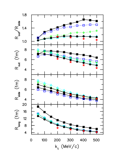
Figure 38: Gaussian HBT radii $R_{\rm out}$, $R_{\rm side}$, and $R_{\rm long}$ from several hydrodynamic calculations explained in the text, together with data from STAR (red stars). Figure reprinted from [299] with permission from the American Physical Society.

Figure 37 shows the HBT radii $R_{\rm side}$, $R_{\rm out}$, $R_{\rm long}$ and the ratio $R_{\rm out}/R_{\rm side}$ for negative pions calculated from (3+1)-dimensional relativistic hydrodynamics for both partial chemical equilibrium (PCE) and chemical equilibrium (CE) in the hadronic phase by Hirano et al. [203]. Except for $R_{\rm long}$ the hydrodynamic calculations fail to reproduce the experimental data quantitatively. $R_{\rm side}$ ($R_{\rm out}$) from the hydrodynamic model underestimates (overestimates) the experimental data. This leads to a large discrepancy in the ratio of $R_{\rm out}/R_{\rm side}$ between hydrodynamic models and experimental data, which is called the HBT puzzle. The same tendency can be seen in other hydrodynamic calculations. At face value this means that the expansion of the fireball happens more rapidly in a shorter time than in hydrodynamic models. Partial chemical equilibrium pushes the hydrodynamic calculations closer to experimental data, however it is not enough to solve the HBT puzzle.

Two improvements are taken into account in Ref. [216]. For one, event-by-event fluctuations in the initial conditions, and secondly continuous emission instead of the sudden freeze-out process which is usually used in hydrodynamic models. The results are shown in Fig. 37. The same radii and ratios as before are shown in four cases: sudden freeze-out with averaged initial condition (FO1), sudden freeze-out with fluctuating initial condition (FO2), continuous emission with averaged initial conditions (CE1) and continuous emission with fluctuating initial conditions (CE2). The realistic treatments of initial conditions and freeze-out bring a significant improvement in $R_{\rm out}$, which also turns into a better agreement of $R_{\rm out}/R_{\rm side}$. However, small discrepancies between hydrodynamic calculations and the experimental data on $R_{\rm out}$ remain.

A solution to the HBT puzzle was finally proposed by Pratt [299]. He suggests that the discrepancies are not from a single shortcoming of hydrodynamic calculations, but from a combination of several effects: mainly prethermalized acceleration, equations of state with inadequate stiffness, and lacking viscosity. Figure 38 shows results from his calculations for the HBT radii together with data from STAR (red stars). The results of many calculations are shown with the extremes being from a hydro calculation with a first-order phase transition without pre-thermal flow and without viscosity (black squares and line), and the gradual improvements culminate in a calculation with stiffer equation of state and pre-thermal flow and viscosities included (black circles and line).

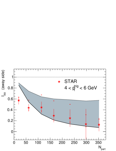
Figure 39: $I_{AA}$ for charged hadrons as a function of $N_{\mathrm{part}}$ with trigger particle having $4<P_{T}<6$ GeV/$c$ compared to data from STAR [300]. Figure reprinted from [124] with kind permission from Springer Science and Business Media.

At high $P_{T}$ 2-particle correlations are measured in heavy ion collisions not for their information on quantum interference but in order to establish kinematic correlations. Di-hadron measurements at RHIC have made it possible to study some properties of jets even though true jet reconstruction is remarkably difficult. Correlation measurements can be recorded by using pairs $T-A$ where $T$ is a trigger hadron and $A$ the associated particle. Most studies at intermediate and high $P_{T}$ have been carried out using such triggered correlations, looking at the per-trigger yield of associated particles

$$Y(P_{T},P_{A},\Delta\phi)=\frac{dN/dP_{T}dP_{A}d(\Delta\phi)}{dN/dP_{T}}$$ (112)

as a function of the relative azimuthal angle $\Delta\phi$ between trigger and associate. Here $P_{T}$ and $P_{A}$ are, in deviation from our usual notation, the transverse momenta of the trigger and associated hadrons, resp. One can then proceed and define a nuclear modification factor for the associated yield

$$I_{AA}=\frac{Y^{AA}(P_{T},P_{A},\Delta\phi)}{Y^{pp}(P_{T},P_{A},\Delta\phi)}\,.$$ (113)

Like $R_{AA}$ we expect $I_{AA}$ to be unity for a loose superposition of proton-proton collisions. Another potentially useful observable are triggered fragmentation functions. They can be derived from per-trigger yields by rewriting the dependence as one on a “momentum fraction” $z=P_{A}/P_{T}$ and integrating over a narrow bin around $\Delta\phi=\pi$.

The amount of data collected on this topic would merit its own review article. We will focus on a few selected examples, mainly to achieve our goal to better constrain the transport coefficient $\hat{q}$. We start by showing the result from Ref. [124] which is now well-known from our discussions on $R_{AA}$ and $v_{2}$. Fig. 39 shows their result for $I_{AA}$ as a function of centrality in the ASW model of energy loss compared to data from STAR. The data fall well into the large error band given by the uncertainty from the reweighted vs the non-reweighted quenching weights.

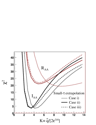
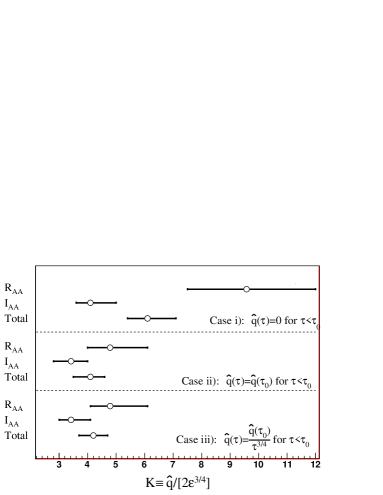
Figure 40: $\chi^{2}$-fits of the parameter $K$ in the ASW model of energy loss from $R_{AA}$ and $I_{AA}$ for three different extrapolations of jet quenching into the pre-equilibrium phase. Figures reprinted from [152] with permission from IOP.

Let us recall the right panel of Fig. 23. In that study the Higher Twist formalism was used together with a calculation of hard processes at NLO accuracy to extract the stopping power $\epsilon_{0}$. As shown in the figure, fitting both $I_{AA}$ and $R_{AA}$ leads to consistent values for $\epsilon_{0}$. This is somewhat different for the recent study by Armesto et al. in the ASW model where the consistency of $\hat{q}$ extracted from $R_{AA}$ and $I_{AA}$ data is very sensitive to details of the modeling [152]. Fig. 40 shows the result for $K=\hat{q}/(2\epsilon^{3/4})$ extracted from $R_{AA}$ and $I_{AA}$ with varying treatments of the quenching during the pre-equilibrium phase. The three cases shown are (i) no quenching before the QGP formation time $\tau_{0}$, (ii) constant $\hat{q}$ for $\tau<\tau_{0}$ and (iii) $\hat{q}$ increasing as $\tau^{-3/4}$ toward $\tau=0$. The results is a reminder that the determination of $\hat{q}$ from data has larger uncertainties.

4.4 Photons

Electromagnetic probes are important means to obtain information from the quark gluon plasma. Photons and lepton pairs carry the information of the whole time-evolution of heavy ion collisions: initial hard collisions, thermalization, expansion, hadronization, and freeze-out. We focus here on photons which encode detailed information of every process which occurs in heavy ion collisions. A schematic account of photon sources has already been given, but we want to list the sources of direct photons once more in one place: (i) prompt hard photons from initial collisions, (ii) vacuum bremsstrahlung (fragmentation) photons, (iii) photons from jet conversions and medium-induced bremsstrahlung (iv) thermal photons from quark gluon plasma (and the hot hadronic phase). This list also orders photons according to which momentum regime they are most important for (from the largest $P_{T}$ to the smallest).

We can deduce the temperature of the fireball from thermal radiation (and check our understanding of the fireball evolution), and we can infer information about the medium density and $\hat{q}$ from jet conversions and induced photon bremsstrahlung. Photons have also great importance as triggers in photon-hadron correlation studies at large $P_{T}$. Triggered fragmentation functions with photon triggers come close to real fragmentation functions since the photon, if the source is dominated by initial hard photons, carries the same transverse momentum as its initial partner parton [115]. This opens a way to measure real medium-modified fragmentation functions, however one has to be cautious because of the many other sources that weaken this kinematic link between the photon and the jet on the other side.

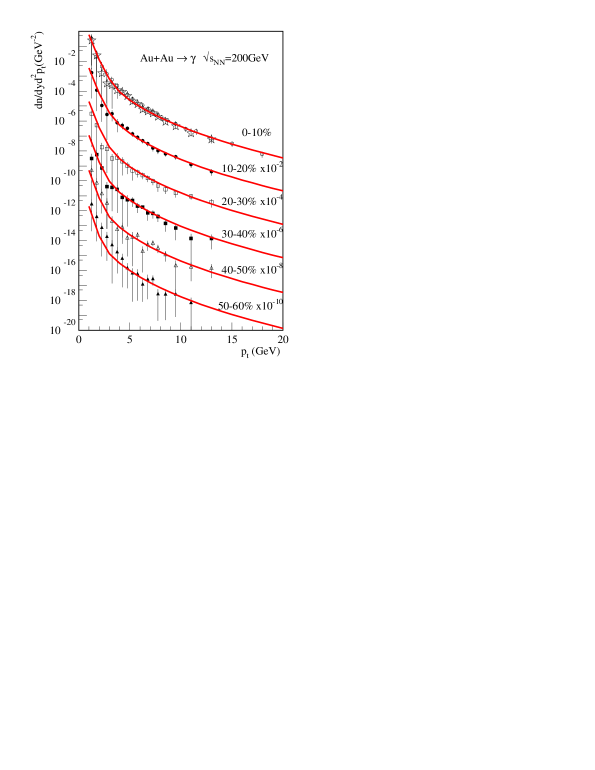
Figure 41: Direct photon production in Au+Au collisions at $\sqrt{s_{NN}}=200$ GeV for five different centrality bins compared to data from PHENIX [302]. Figure reprinted from [301] with permission from the American Physical Society.

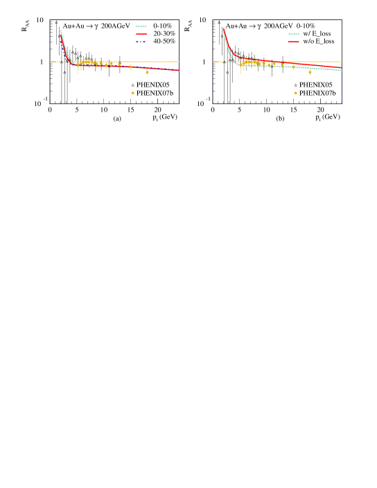
Figure 42: Nuclear modification factor $R_{AA}$ of direct photons as in Fig. 42. Left panel: three different centrality bins are shown. Right panel: calculations with and without energy loss of partons. Figures reprinted from [301] with permission from the American Physical Society.

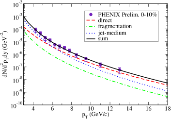
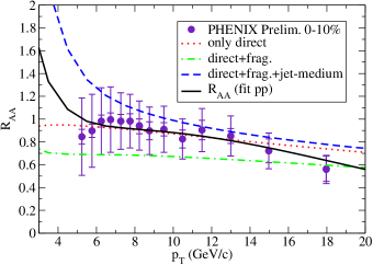
Figure 43: Left panel: direct photon spectra for central Au+Au collisions at RHIC using contributions from hard collisions, bremsstrahlung and jet conversions together with data from PHENIX [304]. Right panel: $R_{AA}$ for direct photons from the same sources. Figures reprinted from [303] with permission from the American Physical Society.

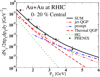
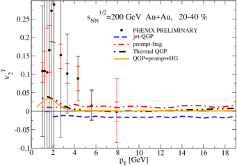
Figure 44: Left panel: Direct photon spectra from all known sources for central Au+Au collisions using the AMY formalism consistently. Right panel: direct photon $v_{2}$ as function of $P_{T}$. Figures reprinted from [305] with permission from the American Physical Society.

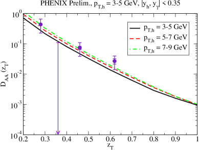
Figure 45: Photon-triggered fragmentation functions $D_{AA}$ for three different trigger windows in the same model as in Fig. 43 compare to data from PHENIX [307]. Figure reprinted from [303] with permission from the American Physical Society.

Figures 42 and 42 show the centrality dependence and the nuclear modification factor of direct photons in Au+Au collisions at $\sqrt{s_{NN}}=200$ GeV, respectively, in the study by Liu et al. [301]. They include all four sources mentioned above and compute thermal radiation by using (3+1)-dimensional hydrodynamic fireball evolution. Their calculation describes the direct photon data from PHENIX very well. The same can be said about the calculation of the McGill group [303]. They use all four sources of photons as well, with energy loss of jets and induced photon bremsstrahlung taken care of by the AMY formalism. A successful fit of hadron and photon data together is hence a crucial consistency test for the AMY formalism. Fig. 43 shows their result for both single inclusive photon spectra and $R_{AA}$ for large and intermediate $P_{T}$ (thermal radiation is therefore omitted in this case).

Fig. 44 shows a calculation of the McGill group including thermal photons according to Arnold, Moore, and Yaffe [305]. In that study the authors also calculated the azimuthal asymmetry $v_{2}$ of direct photons. The $v_{2}$ of thermal photons and of fragmentation photons is expected to be positive, reminiscent of the $v_{2}$ of bulk hadrons and high-$P_{T}$ hadrons respectively. However, photons from jet conversions and induced bremsstrahlung add a negative contribution to the direct photon $v_{2}$ as they are produced more abundantly in the direction where the medium is thicker [306]. The left panel of Fig. 44 shows different contributions to $v_{2}$ with the contribution from jet conversions indeed being negative. Experimental data from PHENIX has been inconclusive so far due to large error bars. Measurements of negative values of $v_{2}$ would be direct evidence for jet conversions.

Fig. 45 shows photon-triggered fragmentation functions $D_{AA}$ obtained from photon-hadron correlations calculated in Ref. [303] with the AMY formalism together with data from PHENIX. This is one of the emerging examples of jet tomography with photon triggers as originally envisioned in [115]. In this study the data is described reasonably well with the parameter in the AMY energy loss (the coupling constant $\alpha_{s}$) set to one consistent value for all observables.

5 Summary and Conclusions

Let us briefly summarize. We have laid out the foundations of perturbative QCD and how they can be used to understand data from the Relativistic Heavy Ion Collider. We explained the concept of collinear factorization widely used in collider physics, and modifications when applied to colliding nuclei. We have then focused on final state interactions, and in particular on leading particle energy loss. Along the way have discussed several popular model calculations for energy loss. We have also pointed out some of their basic assumptions in which they differ. All of them have apparent shortcomings, and even if jet quenching at RHIC is perfectly perturbative, we should not expect all of these calculations to apply. However, all of them explain jet quenching well on a qualitative level. This can be seen positive, we are on the right track, or negative, we are not in a situation where we can confidently falsify one or all of those calculations, due to a long list of uncertainties. We are also not quite ready yet to exclude non-perturbative quenching scenarios from data. In fact, it is very well possible that a mixture of perturbative and non-perturbative quenching co-exist in different temperature ranges.

We showed that all models fit the data on single hadron suppression after adjusting a single parameter, including the systematics of the $P_{T}$- and centrality dependence of $R_{AA}$. On the other hand the quenching strengths extracted from the different models is quite different. The maximum values of $\hat{q}$ in central collisions that have been found lie in the range $\approx 2\ldots 15$ GeV²/fm. Other observables like $v_{2}$ at high $P_{T}$ or $I_{AA}$ have note yet cut down this range as it has become clear that the results are quite sensitive, e.g. to details of the treatment of the underlying fireball.

There is a focused effort to attack the open questions within the framework of the TECHQM collaboration and the newly founded JET collaboration. In the future we need rigorous comparisons and a vetting process of different calculations, a realistic modeling of the fireball and realistic assessments of uncertainties in order to start to falsify certain assumptions and to reduce the error bar on $\hat{q}$. We also have to include more realistic options, like combining perturbative quenching with final state effects in the hadronic phase.

We have also reviewed the successful story of hydrodynamics at RHIC, and the novel developments of the past few years that have brought the first relativistic viscous hydro codes and hybrid models. We have discussed a long list of observables that require the presence of a thermalized and collectively moving quark gluon plasma phase, that can be beautifully explained by hydrodynamic calculations and their extensions. The most convincing single observations are the mass ordering of flow and elliptic flow, and the large size of elliptic flow at RHIC, which are suggested by hydrodynamics and observed in the data. Starting from basic concepts of ideal and viscous hydrodynamics we have moved along a variety of steps that brought vast improvements to our understanding of hydrodynamics, including the arrival of 3+1 dimensional codes, the correct treatment of freeze-out, etc.

Like in the case of pQCD and jet quenching, hydrodynamics has had some difficulties entering a period of precision measurements. Currently, the equation of state from the comparison between hydrodynamic analyses and experimental data favor a first order deconfinement transition, while lattice QCD prefers a crossover transition. Clearly, more systematic phenomenological studies, are needed that try to start from more relaxed assumptions, e.g. by including initial radial flow and dissipative corrections. It is not until both sides, phenomenological analyses of data and theoretical tools like lattice QCD, show the same conclusion that we can pin down the QCD phase diagram. Routine runs of fully 3+1-dimensional, viscous hydrodynamics are around the corner and they should bring us a step closer towards an understanding of QCD thermodynamics and transport coefficients. Current estimates of the shear viscosity range from the 1 to about 4 times the KSS bound of $s/4\pi$.

One of the big challenges in this field is the huge amount of data from RHIC that has remained almost untouched by comprehensive theoretical calculations. There are many results on dihadron azimuthal correlations at high $P_{T}$ [308], three-particle azimuthal correlations, the ridge structure [309], dihadrons with respect to the reaction plane [310], and the emerging full-jet reconstruction [311, 312]. All of these results should fit into a tent anchored on both sides by pQCD and hydrodynamics. Multi-module modeling, carefully tested and endowed with realistic estimates of theoretical uncertainties should eventually be able to explain those features and in the process the data should narrow down the error bars on transport coefficients significantly.

On the experimental side two new challenges will arrive shortly. Energy scans will be conducted at RHIC [313] and supplemented by SPS results and the program at the new FAIR and NICA facilities [314]. These programs will provide new data on the QCD phase diagram at high net baryon densities. Reliable hydro+cascade hybrid models will be given a chance to look for the QCD critical point and a change in the nature of the phase transition. On the other hand the LHC will vastly improve the reach of hard probes by colliding ions at unprecedented center of mass energies. Reconstructed jets and abundant high-$P_{T}$ probes will provide much stricter tests of our understanding of how jets interact with quark gluon plasma.

As the first 10 years of the high energy heavy ion era come to an end we find that we have gained much knowledge. It prepares us for the next decade in which the QCD phase diagram and the quark gluon plasma phase will be mapped out quantitatively.

Acknowledgments

We like to thank R. Rodriguez for many useful discussions. This work was supported by CAREER Award PHY-0847538 from the U. S. National Science Foundation, an Invited Fellowship for Research in Japan by the Japanese Society for the Promotion of Science (JSPS), RIKEN/BNL Research Center, DOE grant DE-AC02-98CH10886, and the Global COE Program “Quest for Fundamental Principles in the Universe” of Nagoya University (G07), Grant-in-Aid for Young Scientists (B) (22740156) and Grant-in-Aid for Scientific Research (S)(22224003) and JSPS Institutional Program for Young Researcher Overseas Visits. R. J. F. would like to express his gratitude to Chiho Nonaka and the Physics Department at Nagoya University for their kind hospitality while part of this work was completed.

References

- [1]
- [2] S. S. Adler et al. [PHENIX Collaboration], Phys. Rev. Lett. 91 (2003) 072301 [arXiv:nucl-ex/0304022]
- [3] J. Adams et al. [STAR Collaboration], Phys. Rev. Lett. 91 (2003) 172302 [arXiv:nucl-ex/0305015]
- [4] First Three Years of Operation of RHIC, Nucl. Phys. A 757 (2005) 1
- [5] B. I. Abelev et al. [STAR Collaboration], Phys. Rev. C 77 (2008) 054901 [arXiv:0801.3466 [nucl-ex]]
- [6] S. Afanasiev et al. [PHENIX Collaboration], Phys. Rev. C 80 (2009) 024909 [arXiv:0905.1070 [nucl-ex]]
- [7] K. Dusling, G. D. Moore and D. Teaney, Phys. Rev. C 81 (2010) 034907 [arXiv:0909.0754 [nucl-th]]
- [8] A. Adare et al. [PHENIX Collaboration], Phys. Rev. Lett. 104 (2010) 132301 [arXiv:0804.4168 [nucl-ex]]
- [9] M. Gyulassy and L. McLerran, Nucl. Phys. A 750 (2005) 30 [arXiv:nucl-th/0405013]
- [10] R. Brock et al. [CTEQ Collaboration], Rev. Mod. Phys. 67 (1995) 157
- [11] A. H. Mueller, Phys. Rep. 73 (1981) 237
- [12] R. K. Ellis, W. Furmanski and R. Petronzio, Nucl. Phys. B 207 (1982) 1
- [13] J. C. Collins, D. E. Soper and G. Sterman, Nucl. Phys. B 261 (1985) 104
- [14] J. C. Collins, D. E. Soper and G. Sterman, Adv. Ser. Direct. High Energy Phys. 5 (1988) 1
- [15] J. W. Qiu and G. Sterman, Nucl. Phys. B 353 (1991) 105
- [16] J. W. Qiu and G. Sterman, Nucl. Phys. B 353 (1991) 137
- [17] A. V. Belitsky, X. Ji and F. Yuan, Nucl. Phys. B 656 (2003) 165 [arXiv:hep-ph/0208038]
- [18] X. d. Ji, J. p. Ma and F. Yuan, Phys. Rev. D 71 (2005) 034005 [arXiv:hep-ph/0404183]
- [19] D. Kharzeev and M. Nardi, Phys. Lett. B 507 (2001) 121 [arXiv:nucl-th/0012025]
- [20] F. Gelis, E. Iancu, J. Jalilian-Marian and R. Venugopalan, preprint arXiv:1002.0333 [hep-ph]
- [21] T. Lappi, preprint arXiv:1003.1852 [hep-ph]
- [22] R. Doria, J. Frenkel and J. C. Taylor, Nucl. Phys. B 168 (1980) 93
- [23] J. F. Owens, Rev. Mod. Phys. 59 (1987) 465
- [24] R. K. Ellis and J. C. Sexton, Rev. Mod. Phys. 269 (1986) 445
- [25] S. D. Ellis, Z. Kunszt and D. E. Soper, Phys. Rev. Lett. 64 (1990) 2121
- [26] S. D. Ellis, Z. Kunszt and D. E. Soper, Phys. Rev. Lett. 69 (1992) 1496
- [27] http://wwwlapp.in2p3.fr/lapth/PHOX_FAMILY/main.html
- [28] G. G. Barnafoldi, G. I. Fai, P. Levai, G. Papp and Y. Zhang, J. Phys. G 27 (2001) 1767 [arXiv:nucl-th/0004066]
- [29] V. N. Gribov and L. N. Lipatov, Sov. J. Nucl. Phys. 15 (1972) 438 , Yad. Fiz. 15 (1972) 781
- [30] G. Altarelli and G. Parisi, Nucl. Phys. B 126 (1977) 298
- [31] Y. L. Dokshitzer, Sov. Phys. JETP 46 (1977) 641 Zh. Eksp. Teor. Fiz. 73 (1977) 1216
- [32] H. L. Lai et al. [CTEQ Collaboration], Eur. Phys. J. C 12 (2000) 375 [arXiv:hep-ph/9903282]
- [33] J. Pumplin, D. R. Stump, J. Huston, H. L. Lai, P. M. Nadolsky and W. K. Tung, JHEP 0207 (2002) 012 [arXiv:hep-ph/0201195]
- [34] A. D. Martin, R. G. Roberts, W. J. Stirling and R. S. Thorne, Phys. Lett. B 531 (2002) 216 [arXiv:hep-ph/0201127]
- [35] A. D. Martin, W. J. Stirling and R. S. Thorne, Phys. Lett. B 636 (2006) 259 [arXiv:hep-ph/0603143]
- [36] http://durpdg.dur.ac.uk/hepdata/pdf.html
- [37] J. C. Collins and D. E. Soper, Nucl. Phys. B 194 (1982) 445
- [38] B. A. Kniehl, G. Kramer and B. Potter, Nucl. Phys. B 582 (2000) 514 [arXiv:hep-ph/0010289]
- [39] S. Albino, B. A. Kniehl and G. Kramer, Nucl. Phys. B 725 (2005) 181 [arXiv:hep-ph/0502188]
- [40] M. Hirai, S. Kumano, T. H. Nagai and K. Sudoh, Phys. Rev. D 75 (2007) 094009 [arXiv:hep-ph/0702250]
- [41] D. de Florian, R. Sassot and M. Stratmann, Phys. Rev. D 75 (2007) 114010 [arXiv:hep-ph/0703242]
- [42] D. de Florian, R. Sassot and M. Stratmann, Phys. Rev. D 76 (2007) 074033 [arXiv:0707.1506 [hep-ph]]
- [43] L. Bourhis, M. Fontannaz and J. P. Guillet, Eur. Phys. J. C 2 (1998) 529 [arXiv:hep-ph/9704447]
- [44] P. Aurenche, A. Douiri, R. Baier, M. Fontannaz and D. Schiff, Phys. Lett. B 140 (1984) 87
- [45] E. L. Berger, E. Braaten and R. D. Field, Nucl. Phys. B 239 (1984) 52
- [46] P. Aurenche, M. Fontannaz, J. P. Guillet, B. A. Kniehl, E. Pilon and M. Werlen, Eur. Phys. J. C 9 (1999) 107 [arXiv:hep-ph/9811382]
- [47] E. Laenen, G. Sterman and W. Vogelsang, Phys. Rev. Lett. 84 (2000) 4296 [arXiv:hep-ph/0002078]
- [48] G. Sterman and W. Vogelsang, Phys. Rev. D 71 (2005) 014013 [arXiv:hep-ph/0409234]
- [49] J. I. Kapusta, P. Lichard and D. Seibert, Phys. Rev. D 44 (1991) 2774 [Erratum-ibid. Phys. Rev. D 47 (1993) 4171 ]
- [50] R. Baier, H. Nakkagawa, A. Niegawa and K. Redlich, Z. Phys. C 53 (1992) 433
- [51] P. Aurenche, F. Gelis, R. Kobes and H. Zaraket, Phys. Rev. D 58 (1998) 085003 [arXiv:hep-ph/9804224]
- [52] P. B. Arnold, G. D. Moore and L. G. Yaffe, JHEP 0111 (2001) 057 [arXiv:hep-ph/0109064]
- [53] P. B. Arnold, G. D. Moore and L. G. Yaffe, JHEP 0112 (2001) 009 [arXiv:hep-ph/0111107]
- [54] S. A. Bass, B. Muller and D. K. Srivastava, Phys. Rev. Lett. 90 (2003) 082301 [arXiv:nucl-th/0209030]
- [55] J. J. Aubert et al. [European Muon Collaboration], Phys. Lett. B 123 (1983) 275
- [56] S. V. Akulinichev, S. Shlomo, S. A. Kulagin and G. M. Vagradov, Phys. Rev. Lett. 55 (1985) 2239
- [57] L. L. Frankfurt and M. I. Strikman, Phys. Rept. 160 (1988) 235
- [58] N. Armesto, J. Phys. G 32 (2006) R367 [arXiv:hep-ph/0604108]
- [59] K. J. Eskola, V. J. Kolhinen and C. A. Salgado, Eur. Phys. J. C 9 (1999) 61 [arXiv:hep-ph/9807297]
- [60] K. J. Eskola, V. J. Kolhinen, H. Paukkunen and C. A. Salgado, JHEP 0705 (2007) 002 [arXiv:hep-ph/0703104]
- [61] K. J. Eskola, H. Paukkunen and C. A. Salgado, JHEP 0807 (2008) 102 [arXiv:0802.0139 [hep-ph]]
- [62] K. J. Eskola, H. Paukkunen and C. A. Salgado, JHEP 0904 (2009) 065 [arXiv:0902.4154 [hep-ph]]
- [63] M. Hirai, S. Kumano and M. Miyama, Phys. Rev. D 64 (2001) 034003 [arXiv:hep-ph/0103208]
- [64] M. Hirai, S. Kumano and T. H. Nagai, Phys. Rev. C 70 (2004) 044905 [arXiv:hep-ph/0404093]
- [65] M. Hirai, S. Kumano and T. H. Nagai, Phys. Rev. C 76 (2007) 065207 [arXiv:0709.3038 [hep-ph]]
- [66] D. de Florian and R. Sassot, Phys. Rev. D 69 (2004) 074028 [arXiv:hep-ph/0311227]
- [67] R. L. Jaffe, in Lectures on QCD, (Ed. F. Lenz) Preprint arXiv:hep-ph/9602236
- [68] M. Luo, J. w. Qiu and G. Sterman, Phys. Lett. B 279 (1992) 377
- [69] M. Luo, J. w. Qiu and G. Sterman, Phys. Rev. D 49 (1994) 4493
- [70] M. Luo, J. w. Qiu and G. Sterman, Phys. Rev. D 50 (1994) 1951
- [71] X. f. Guo, Nucl. Phys. A 638 (1998) 539C [arXiv:hep-ph/9801450]
- [72] R. J. Fries, B. Müller, A. Schafer and E. Stein, Phys. Rev. Lett. 83 (1999) 4261 [arXiv:hep-ph/9907567]
- [73] R. J. Fries, A. Schäfer, E. Stein and B. Müller, Nucl. Phys. B 582 (2000) 537 [arXiv:hep-ph/0002074]
- [74] R. J. Fries, Phys. Rev. D 68 (2003) 074013 [arXiv:hep-ph/0209275]
- [75] A. Majumder and B. Muller, Phys. Rev. C 77 (2008) 054903 [arXiv:0705.1147 [nucl-th]]
- [76] X. F. Guo, J. W. Qiu and W. Zhu, Phys. Lett. B 523 (2001) 88 [arXiv:hep-ph/0110038]
- [77] X. F. Guo, Phys. Rev. D 58 (1998) 114033 [arXiv:hep-ph/9804234]
- [78] X. F. Guo and J. W. Qiu, Phys. Rev. D 53 (1996) 6144 [arXiv:hep-ph/9512262]
- [79] A. Majumder, R. J. Fries and B. Muller, Phys. Rev. C 77 (2008) 065209 [arXiv:0711.2475 [nucl-th]]
- [80] J. W. Cronin, H. J. Frisch, M. J. Shochet, J. P. Boymond, R. Mermod, P. A. Piroue and R. L. Sumner, Phys. Rev. D 11 (1975) 3105
- [81] A. Accardi et al., CERN Yellow Report Hard Probes in Heavy Ion Collisions at the LHC: PDFs, Shadowing and p+A Collisions, CERN Yellow Report, arXiv:hep-ph/0308248; see also A. Accardi, preprint arXiv:hep-ph/0212148
- [82] A. Accardi and M. Gyulassy, Phys. Lett. B 586 (2004) 244 [arXiv:nucl-th/0308029]
- [83] M. B. Johnson, B. Z. Kopeliovich and I. Schmidt, Phys. Rev. C 75 (2007) 064905 [arXiv:hep-ph/0701015]
- [84] J. Jalilian-Marian, Y. Nara and R. Venugopalan, Phys. Lett. B 577 (2003) 54 [arXiv:nucl-th/0307022]
- [85] D. Kharzeev, Y. V. Kovchegov and K. Tuchin, Phys. Rev. D 68 (2003) 094013 [arXiv:hep-ph/0307037]
- [86] A. Airapetian et al. [HERMES Collaboration], Nucl. Phys. B 780 (2007) 1 [arXiv:0704.3270 [hep-ex]]
- [87] X. F. Guo and X. N. Wang, Phys. Rev. Lett. 85 (2000) 3591 [arXiv:hep-ph/0005044]
- [88] P. Levai, G. G. Barnafoldi, G. Fai and G. Papp, Nucl. Phys. A 783 (2007) 101 [arXiv:nucl-th/0611007]
- [89] H. Buesching, Eur. Phys. J. C 49 (2006) 41
- [90] S. Y. Li and X. N. Wang, Phys. Lett. B 527 (2002) 85 [arXiv:nucl-th/0110075]
- [91] J. D. Bjorken, preprint FERMILAB-PUB-82-059-THY, (1982)
- [92] M. H. Thoma and M. Gyulassy, Nucl. Phys. B 351 (1991) 491
- [93] M. Gyulassy and X. N. Wang, Nucl. Phys. B 420 (1994) 583 [arXiv:nucl-th/9306003]
- [94] X. N. Wang, M. Gyulassy and M. Plumer, Phys. Rev. D 51 (1995) 3436 [arXiv:hep-ph/9408344]
- [95] R. Baier, Y. L. Dokshitzer, A. H. Mueller, S. Peigne and D. Schiff, Nucl. Phys. B 483 (1997) 291 [arXiv:hep-ph/9607355]
- [96] R. Baier, Y. L. Dokshitzer, A. H. Mueller, S. Peigne and D. Schiff, Nucl. Phys. B 484 (1997) 265 [arXiv:hep-ph/9608322]
- [97] B. G. Zakharov, JETP Lett. 63 (1996) 952 [arXiv:hep-ph/9607440]
- [98] B. G. Zakharov, JETP Lett. 65 (1997) 615 [arXiv:hep-ph/9704255]
- [99] A. Majumder and M. Van Leeuwen, Prog. Part. Nucl. Phys., in print [arXiv:1002.2206 [hep-ph]]
- [100] L. D. Landau and I. Pomeranchuk, Dokl. Akad. Nauk Ser. Fiz. 92 (1953) 535
- [101] A. B. Migdal, Phys. Rev. 103 (1956) 1811
- [102] X. N. Wang and X. F. Guo, Nucl. Phys. A 696 (2001) 788 [arXiv:hep-ph/0102230]
- [103] P. B. Arnold, G. D. Moore and L. G. Yaffe, JHEP 0206 (2002) 030 [arXiv:hep-ph/0204343]
- [104] S. Jeon and G. D. Moore, Phys. Rev. C 71 (2005) 034901 [arXiv:hep-ph/0309332]
- [105] C. A. Salgado and U. A. Wiedemann, Phys. Rev. Lett. 89 (2002) 092303 [arXiv:hep-ph/0204221]
- [106] C. A. Salgado and U. A. Wiedemann, Phys. Rev. D 68 (2003) 014008 [arXiv:hep-ph/0302184]
- [107] M. Gyulassy, P. Levai and I. Vitev, Nucl. Phys. B 571 (2000) 197 [arXiv:hep-ph/9907461]
- [108] M. Gyulassy, P. Levai and I. Vitev, Phys. Rev. Lett. 85 (2000) 5535 [arXiv:nucl-th/0005032]
- [109] M. Gyulassy, P. Levai and I. Vitev, Nucl. Phys. B 594 (2001) 371 [arXiv:nucl-th/0006010]
- [110] R. J. Fries, preprint arXiv:hep-ph/0201311
- [111] A. Schafer, X. N. Wang and B. W. Zhang, Nucl. Phys. A 793 (2007) 128 [arXiv:0704.0106 [hep-ph]]
- [112] W. T. Deng and X. N. Wang, Phys. Rev. C 81 (2010) 024902 [arXiv:0910.3403 [hep-ph]]
- [113] E. Wang and X. N. Wang, Phys. Rev. Lett. 89 (2002) 162301 [arXiv:hep-ph/0202105]
- [114] A. Airapetian et al. [HERMES Collaboration], Phys. Lett. B 577 (2003) 37 [arXiv:hep-ex/0307023]
- [115] X. N. Wang, Z. Huang and I. Sarcevic, Phys. Rev. Lett. 77 (1996) 231 [arXiv:hep-ph/9605213]
- [116] A. Majumder, E. Wang and X. N. Wang, Phys. Rev. Lett. 99 (2007) 152301 [arXiv:nucl-th/0412061]
- [117] A. Majumder, Phys. Rev. C 80 (2009) 031902 [arXiv:0810.4967 [nucl-th]]
- [118] A. Majumder, preprint arXiv:0912.2987 [nucl-th]
- [119] M. Gyulassy, P. Levai and I. Vitev, Phys. Lett. B 538 (2002) 282 [arXiv:nucl-th/0112071]
- [120] M. Gyulassy, P. Levai and I. Vitev, Phys. Rev. D 66 (2002) 014005 [arXiv:nucl-th/0201078]
- [121] S. Wicks, W. Horowitz, M. Djordjevic and M. Gyulassy, Nucl. Phys. A 784 (2007) 426 [arXiv:nucl-th/0512076]
- [122] U. A. Wiedemann, Nucl. Phys. A 690 (2001) 731 [arXiv:hep-ph/0008241]
- [123] U. A. Wiedemann, Nucl. Phys. B 588 (2000) 303 [arXiv:hep-ph/0005129]
- [124] A. Dainese, C. Loizides and G. Paic, Eur. Phys. J. C 38 (2005) 461 [arXiv:hep-ph/0406201]
- [125] http://csalgado.web.cern.ch/csalgado/Carlos_A._Salgado.html
- [126] R. Baier, Nucl. Phys. A 715 (2003) 209 [arXiv:hep-ph/0209038]
- [127] M. Cacciari and G. P. Salam, Phys. Lett. B 641 (2006) 57 [arXiv:hep-ph/0512210]
- [128] G. P. Salam and G. Soyez, JHEP 0705 (2007) 086 [arXiv:0704.0292 [hep-ph]]
- [129] M. Cacciari, G. P. Salam and G. Soyez, JHEP 0804 (2008) 063 [arXiv:0802.1189 [hep-ph]]
- [130] I. P. Lokhtin and A. M. Snigirev, Eur. Phys. J. C 45 (2006) 211 [arXiv:hep-ph/0506189]
- [131] N. Armesto, L. Cunqueiro and C. A. Salgado, Eur. Phys. J. C 63 (2009) 679 [arXiv:0907.1014 [hep-ph]]
- [132] K. Zapp, G. Ingelman, J. Rathsman, J. Stachel and U. A. Wiedemann, Eur. Phys. J. C 60 (2009) 617 [arXiv:0804.3568 [hep-ph]]
- [133] T. Renk, Phys. Rev. C 78 (2008) 034908 [arXiv:0806.0305 [hep-ph]]
- [134] B. Schenke, C. Gale and S. Jeon, Phys. Rev. C 80 (054913) , 2009 [arXiv:0909.2037 [hep-ph]]
- [135] I. Vitev, S. Wicks and B. W. Zhang, JHEP 0811 (2008) 093 [arXiv:0810.2807 [hep-ph]]
- [136] S. Sapeta and U. A. Wiedemann, Eur. Phys. J. C 55 (2008) 293 [arXiv:0707.3494 [hep-ph]]
- [137] C. M. Ko, W. Liu and B. W. Zhang, Few Body Syst. 41 (2007) 63
- [138] W. Liu and R. J. Fries, Phys. Rev. C 77 (2008) 054902 [arXiv:0801.0453 [nucl-th]]
- [139] W. Liu and R. J. Fries, Phys. Rev. C 78 (2008) 037902 [arXiv:0805.1093 [nucl-th]]
- [140] W. Liu and R. J. Fries, preprint arXiv:0805.3721 [nucl-th]
- [141] L. Ruan [for the STAR Collaboration], J. Phys. G 37 (2010) 094013 [arXiv:1001.3347 [nucl-ex]]
- [142] R. J. Fries, B. Muller and D. K. Srivastava, Phys. Rev. Lett. 90 (2003) 132301 [arXiv:nucl-th/0208001]
- [143] R. J. Fries, B. Muller and D. K. Srivastava, Phys. Rev. C 72 (2005) 041902 [arXiv:nucl-th/0507018]
- [144] S. Turbide, C. Gale, S. Jeon and G. D. Moore, Phys. Rev. C 72 (2005) 014906 [arXiv:hep-ph/0502248]
- [145] D. K. Srivastava, C. Gale and R. J. Fries, Phys. Rev. C 67 (2003) 034903 [arXiv:nucl-th/0209063]
- [146] S. Turbide, C. Gale, D. K. Srivastava and R. J. Fries, Phys. Rev. C 74 (2006) 014903 [arXiv:hep-ph/0601042]
- [147] C. P. Herzog, A. Karch, P. Kovtun, C. Kozcaz and L. G. Yaffe, JHEP 0607 (2006) 013 [arXiv:hep-th/0605158]
- [148] H. Liu, K. Rajagopal and U. A. Wiedemann, Phys. Rev. Lett. 97 (2006) 182301 [arXiv:hep-ph/0605178]
- [149] S. S. Gubser, Phys. Rev. D 74 (2006) 126005 [arXiv:hep-th/0605182]
- [150] W. A. Horowitz and M. Gyulassy, Phys. Lett. B 666 (2008) 320 [arXiv:0706.2336 [nucl-th]]
- [151] J. Liao and E. Shuryak, Phys. Rev. Lett. 102 (2009) 202302 [arXiv:0810.4116 [nucl-th]]
- [152] N. Armesto, M. Cacciari, T. Hirano, J. L. Nagle and C. A. Salgado, J. Phys. G 37 (2010) 025104 [arXiv:0907.0667 [hep-ph]]
- [153] S. A. Bass, C. Gale, A. Majumder, C. Nonaka, G. Y. Qin, T. Renk and J. Ruppert, Phys. Rev. C 79 (2009) 024901 [arXiv:0808.0908 [nucl-th]]
- [154] R. Rodriguez, R. J. Fries and E. Ramirez, Phys. Lett. B 693 (2010) 108 [arXiv:1005.3567 [nucl-th]]
- [155] O. Fochler, Z. Xu and C. Greiner, Phys. Rev. C 82 (2010) 024907 [arXiv:1003.4380 [hep-ph]]
- [156] J. Casalderrey-Solana, E. V. Shuryak and D. Teaney, Nucl. Phys. A 774 (2006) 577 [arXiv:hep-ph/0411315]
- [157] R. B. Neufeld, B. Muller and J. Ruppert, Phys. Rev. C 78 (2008) 041901 [arXiv:0802.2254 [hep-ph]]
- [158] B. Betz, M. Gyulassy, D. H. Rischke, H. Stocker and G. Torrieri, J. Phys. G 35 (2008) 104106 [arXiv:0804.4408 [hep-ph]]
- [159] P. B. Arnold, Phys. Rev. D 80 (2009) 025004 [arXiv:0903.1081 [nucl-th]]
- [160] S .Z. Belenkij, L. D. Landau, Nuovo Cim. Suppl. 3S10 (1956) 15 , Usp. Fiz. Nauk 56 (1955) 309
- [161] J. D. Bjorken, Phys. Rev. D 27 (1983) 140
- [162] E. Schnedermann, J. Sollfrank and U. W. Heinz, Phys. Rev. C 48 (1993) 2462 [arXiv:nucl-th/9307020]
- [163] H. Appelshauser et al. [NA49 Collaboration], Phys. Rev. Lett. 80 (1998) 4136 [arXiv:nucl-ex/9711001]
- [164] C. Alt et al. [NA49 Collaboration], Phys. Rev. C 68 (2003) 034903 [arXiv:nucl-ex/0303001]
- [165] P. F. Kolb, P. Huovinen, U. W. Heinz and H. Heiselberg, Phys. Lett. B 500 (2001) 232 [arXiv:hep-ph/0012137]
- [166] P. Huovinen, P. F. Kolb, U. W. Heinz, P. V. Ruuskanen and S. A. Voloshin, Phys. Lett. B 503 (2001) 58 [arXiv:hep-ph/0101136]
- [167] Quark-Gluon Plasma, Nucl. Phys. A 750 (2005) 1
- [168] T. Hirano and M. Gyulassy, Nucl. Phys. A 769 (2006) 71 [arXiv:nucl-th/0506049]
- [169] R. S. Bhalerao, J. P. Blaizot, N. Borghini and J. Y. Ollitrault, Phys. Lett. B 627 (2005) 49 [arXiv:nucl-th/0508009]
- [170] Y. Aoki, G. Endrodi, Z. Fodor, S. D. Katz and K. K. Szabo, Nature4436752006 [arXiv:hep-lat/0611014]
- [171] P. Petreczky, Nucl. Phys. A 830 (2009) 11C [arXiv:0908.1917 [hep-ph]]
- [172] I. Müller, Z. Phys. 198 (1967) 329
- [173] W. Israel, Ann. Phys. (N.Y.) 100 (1976) 310
- [174] W. Israel and J. M. Stewart, Phys. Lett. A 58 (1976) 213
- [175] W. Israel and J. M. Stewart, Ann. Phys. (N.Y.) 118 (1979) 341
- [176] M. Grmela and H. C. Öttinger, Phys. Rev. E 56 (1997) 6620
- [177] H. C. Öttinger and M. Grmela, Phys. Rev. E 56 (1997) 6633
- [178] H. C. Öttinger, Phys. Rev. E 57 (1998) 1416
- [179] D. A. Teaney, preprint arXiv:0905.2433 [nucl-th]
- [180] A. Muronga and D. H. Rischke, preprint arXiv:nucl-th/0407114
- [181] K. Dusling and D. Teaney, Phys. Rev. C 77 (2008) 034905 [arXiv:0710.5932 [nucl-th]]
- [182] R. Baier, P. Romatschke, D. T. Son, A. O. Starinets and M. A. Stephanov, JHEP 0804 (2008) 100 [arXiv:0712.2451 [hep-th]]
- [183] B. Betz, D. Henkel and D. H. Rischke, J. Phys. G 36 (2009) 064029
- [184] T. Tsumura, T. Kunihiro and K. Ohnishi, Phys. Lett. B 646 (2007) 132
- [185] K. Tsumura and T. Kunihiro, Phys. Lett. B 668 (2008) 425 [arXiv:0709.3645 [nucl-th]]
- [186] R. J. Fries, B. Muller and A. Schafer, Phys. Rev. C 78 (2008) 034913 [arXiv:0807.4333 [nucl-th]]
- [187] H. Song and U. W. Heinz, Phys. Lett. B 693 (2010) 108 [arXiv:0909.1549 [nucl-th]]
- [188] J. P. Boris, and D. L. Book, J. Comput. Phys. 11 (1973) 38
- [189] V. Schneider, U. Katscher, D. H. Rischke, B. Waldhauser, J. A. Maruhn and C. D. Munz, J. Comput. Phys. 105 (1993) 92
- [190] R. Andrade, F. Grassi, Y. Hama, T. Kodama and O. J. Socolowski, Phys. Rev. Lett. 97 (2006) 202302 [arXiv:nucl-th/0608067]
- [191] C. E. Aguiar, T. Kodama, T. Osada and Y. Hama, J. Phys. G 27 (2001) 75 [arXiv:hep-ph/0006239]
- [192] C. Nonaka and S. A. Bass, Phys. Rev. C 75 (2007) 014902 [arXiv:nucl-th/0607018]
- [193] H. Song and U. W. Heinz, Phys. Rev. C 78 (2008) 024902 [arXiv:0805.1756 [nucl-th]]
- [194] A. K. Chaudhuri, J. Phys. G 37 (2010) 075011 [arXiv:0910.0979 [nucl-th]]
- [195] G. S. Denicol, T. Kodama, T. Koide and Ph. Mota, J. Phys. G 36 (2009) 035103
- [196] E. Molnar, H. Niemi and D. H. Rischke, Eur. Phys. J. C 65 (2010) 615 [arXiv:0907.2583 [nucl-th]]
- [197] J. Adams et al. [STAR Collaboration], Phys. Rev. Lett. 92 (2004) 182301 [arXiv:nucl-ex/0307024]
- [198] D. Molnar and P. Huovinen, Phys. Rev. Lett. 94 (2005) 012302 [arXiv:nucl-th/0404065]
- [199] H. J. Drescher, A. Dumitru, C. Gombeaud and J. Y. Ollitrault, Phys. Rev. C 76 (2007) 024905 [arXiv:0704.3553 [nucl-th]]
- [200] R. Baier, A. H. Mueller, D. Schiff and D. T. Son, Phys. Lett. B 502 (2001) 51 [arXiv:hep-ph/0009237]
- [201] S. Mrowczynski, PoS CPOD2006 (2006) 042 [arXiv:hep-ph/0611067]
- [202] P. F. Kolb, U. W. Heinz, P. Huovinen, K. J. Eskola and K. Tuominen, Nucl. Phys. A 696 (2001) 197 [arXiv:hep-ph/0103234]
- [203] T. Hirano and K. Tsuda, Phys. Rev. C 66 (2002) 054905 [arXiv:nucl-th/0205043]
- [204] D. Teaney, J. Lauret and E. V. Shuryak, Phys. Rev. Lett. 86 (2001) 4783 [arXiv:nucl-th/0011058]; preprint: nucl-th/0110037
- [205] S. S. Adler et al. [PHENIX Collaboration], Phys. Rev. Lett. 91 (2003) 072303 [arXiv:nucl-ex/0306021]
- [206] P. F. Kolb and R. Rapp, Phys. Rev. C 67 (2003) 044903 [arXiv:hep-ph/0210222]
- [207] T. Renk, Phys. Rev. C 70 (2004) 021903 [arXiv:hep-ph/0404140]
- [208] T. Renk, Phys. Rev. C 69 (2004) 044902 [arXiv:hep-ph/0310346]
- [209] U. W. Heinz and P. F. Kolb, preprint arXiv:hep-ph/0204061
- [210] M. Luzum and P. Romatschke, Phys. Rev. C 78 (2008) 034915 [Erratum-ibid. Phys. Rev. C 79 (2009) 039903 ] [arXiv:0804.4015 [nucl-th]]
- [211] T. Hirano and Y. Nara, Nucl. Phys. A 743 (2004) 305 [arXiv:nucl-th/0404039]
- [212] T. Hirano, U. W. Heinz, D. Kharzeev, R. Lacey and Y. Nara, Phys. Lett. B 636 (2006) 299 [arXiv:nucl-th/0511046]
- [213] L. P. Csernai, Y. Cheng, S. Horvat, V. Magas, D. Strottman and M. Zetenyi, J. Phys. G 36 (2009) 064032
- [214] K. J. Eskola, H. Honkanen, H. Niemi, P. V. Ruuskanen and S. S. Rasanen, Phys. Rev. C 72 (2005) 044904 [arXiv:hep-ph/0506049]
- [215] Y. Hama, T. Kodama and O. J. Socolowski, Braz. J. Phys. 35 (2005) 24 [arXiv:hep-ph/0407264]
- [216] O. J. Socolowski, F. Grassi, Y. Hama and T. Kodama, Phys. Rev. Lett. 93 (2004) 182301 [arXiv:hep-ph/0405181]
- [217] S. Borsanyi et al., Preprint arXiv:1007.2580 [hep-lat]
- [218] P. Huovinen, Nucl. Phys. A 761 (2005) 296 [arXiv:nucl-th/0505036]
- [219] P. Huovinen and P. Petreczky, Nucl. Phys. A 837 (2010) 26 [arXiv:0912.2541 [hep-ph]]
- [220] M. A. Stephanov, K. Rajagopal and E. V. Shuryak, Phys. Rev. Lett. 81 (1998) 4816 [arXiv:hep-ph/9806219]
- [221] M. A. Stephanov, PoS LAT2006 (2006) 024 [arXiv:hep-lat/0701002]
- [222] P. de Forcrand and O. Philipsen, PoS LATTICE2008 (2008) 208 [arXiv:0811.3858 [hep-lat]]
- [223] C. Nonaka, B. Muller, S. A. Bass and M. Asakawa, Phys. Rev. C 71 (2005) 051901 [arXiv:nucl-th/0501028]
- [224] M. Asakawa, S. A. Bass, B. Muller and C. Nonaka, Phys. Rev. Lett. 101 (2008) 122302 [arXiv:0803.2449 [nucl-th]]
- [225] A. Nakamura and S. Sakai, Phys. Rev. Lett. 94 (2005) 072305 [arXiv:hep-lat/0406009]
- [226] H. B. Meyer, Phys. Rev. D 76 (2007) 101701 [arXiv:0704.1801 [hep-lat]]
- [227] P. B. Arnold, G. D. Moore and L. G. Yaffe, JHEP 0011 (2000) 001 [arXiv:hep-ph/0010177]
- [228] P. B. Arnold, G. D. Moore and L. G. Yaffe, JHEP 0305 (2003) 051 [arXiv:hep-ph/0302165]
- [229] P. B. Arnold, C. Dogan and G. D. Moore, Phys. Rev. D 74 (2006) 085021 [arXiv:hep-ph/0608012]
- [230] A. Muronga, Phys. Rev. C 69 (2004) 044901 [arXiv:nucl-th/0309056]
- [231] S. Muroya and N. Sasaki, Prog. Theor. Phys. 113 (2005) 457 [arXiv:nucl-th/0408055]
- [232] N. Demir and S. A. Bass, Phys. Rev. Lett. 102 (2009) 172302 [arXiv:0812.2422 [nucl-th]]
- [233] Z. Xu and C. Greiner, Phys. Rev. Lett. 100 (2008) 172301 [arXiv:0710.5719 [nucl-th]]
- [234] Z. Xu, C. Greiner and H. Stocker, Phys. Rev. Lett. 101 (2008) 082302 [arXiv:0711.0961 [nucl-th]]
- [235] D. Molnar and M. Gyulassy, Nucl. Phys. A 697 (2002) 495 [Erratum-ibid. A 703 (2002) 893] [arXiv:nucl-th/0104073]
- [236] Z. Xu and C. Greiner, Phys. Rev. C 71 (2005) 064901 [arXiv:hep-ph/0406278]
- [237] Z. Xu and C. Greiner, Phys. Rev. C 76 (2007) 024911 [arXiv:hep-ph/0703233]
- [238] Z. Xu and C. Greiner, Phys. Rev. C 79 (2009) 014904 [arXiv:0811.2940 [hep-ph]]
- [239] See e.g. P. Braun-Munzinger, K. Redlich, J. Stachel, in Quark Gluon Plasma 3, (Eds. R. C. Hwa and X. N. Wang, World Scientific)
- [240] F. Cooper, G. Frye, Phys. Rev. D 10 (1974) 186
- [241] J.-P. Blaizot, J.-Y. Ollitrault, in Quark-Gluon Plasma, (Ed. R. C. Hwa, World Scientific) Adv.Ser.Direct.High Energy Phys.63931990
- [242] J. Adams et al. [STAR Collaboration], Phys. Rev. Lett. 92 (2004) 112301 [arXiv:nucl-ex/0310004]
- [243] U. W. Heinz and P. F. Kolb, Nucl. Phys. A 702 (2002) 269 [arXiv:hep-ph/0111075]
- [244] N. Arbex, F. Grassi, Y. Hama, O. Socolowski, preprint arXiv:nucl-th/0102056
- [245] N. Arbex, F. Grassi, Y. Hama and O. Socolowski, Phys. Rev. C 64 (2001) 064906
- [246] D. Teaney, preprint nucl-th/0204023
- [247] S. A. Bass and A. Dumitru, Phys. Rev. C 61 (2000) 064909 [arXiv:nucl-th/0001033]
- [248] M. Laine and Y. Schroder, Phys. Rev. D 73 (2006) 085009 [arXiv:hep-ph/0603048].
- [249] https://wiki.bnl.gov/TECHQM/index.php/Main_Page
- [250] H. Petersen, J. Steinheimer, G. Burau, M. Bleicher and H. Stocker, Phys. Rev. C 78 (2008) 044901 [arXiv:0806.1695 [nucl-th]]
- [251] K. Werner, T. Hirano, I. Karpenko, T. Pierog, S. Porteboeuf, M. Bleicher and S. Haussler, J. Phys. G 36 (2009) 064030
- [252] R. J. Fries, B. Muller, C. Nonaka and S. A. Bass, Phys. Rev. Lett. 90 (2003) 202303 [arXiv:nucl-th/0301087]
- [253] R. J. Fries, B. Muller, C. Nonaka and S. A. Bass, Phys. Rev. C 68 (2003) 044902 [arXiv:nucl-th/0306027]
- [254] V. Greco, C. M. Ko and P. Levai, Phys. Rev. Lett. 90 (2003) 202302 [arXiv:nucl-th/0301093]
- [255] V. Greco, C. M. Ko and P. Levai, Phys. Rev. C 68 (2003) 034904 [arXiv:nucl-th/0305024]
- [256] B. Muller, R. J. Fries and S. A. Bass, Phys. Lett. B 618 (2005) 77 [arXiv:nucl-th/0503003]
- [257] L. Ravagli and R. Rapp, Phys. Lett. B 655 (2007) 126 [arXiv:0705.0021 [hep-ph]]
- [258] R. J. Fries, S. A. Bass and B. Muller, Phys. Rev. Lett. 94 (2005) 122301 [arXiv:nucl-th/0407102]
- [259] L. Ravagli, H. van Hees and R. Rapp, Phys. Rev. C 79 (2009) 064902 [arXiv:0806.2055 [hep-ph]].
- [260] M. He, R. J. Fries and R. Rapp, arXiv:1006.1111 [nucl-th]
- [261] R. C. Hwa and C. B. Yang, Phys. Rev. C 70 (2004) 024904 [arXiv:hep-ph/0312271]
- [262] R. C. Hwa and C. B. Yang, Phys. Rev. C 70 (2004) 024905 [arXiv:nucl-th/0401001]
- [263] A. Majumder, E. Wang and X. N. Wang, Phys. Rev. C 73 (2006) 044901 [arXiv:nucl-th/0506040]
- [264] K. S. Lee, S. Bass, B. Muller and C. Nonaka, J. Phys. G 36 (2009) 064034 [arXiv:0812.4724 [nucl-th]]
- [265] R. J. Fries, V. Greco and P. Sorensen, Ann. Rev. Nucl. Part. Sci. 58 (2008) 177 [arXiv:0807.4939 [nucl-th]]
- [266] R. J. Fries, J. Phys. G 30 (2004) S853 [arXiv:nucl-th/0403036]
- [267] F. Becattini and R. Fries, in Relativistic Heavy Ion Physics, Landolt Börnstein: New Series, I-23, [arXiv:0907.1031 [nucl-th]]
- [268] T. Hirano and Y. Nara, Phys. Rev. C 69 (2004) 034908 [arXiv:nucl-th/0307015]
- [269] B. I. Abelev et al. [STAR Collaboration], Phys. Rev. C 79 (2009) 064903 [arXiv:0809.4737 [nucl-ex]]
- [270] C. Nonaka, R. J. Fries and S. A. Bass, Phys. Lett. B 583 (2004) 73 [arXiv:nucl-th/0308051]
- [271] B. B. Back et al. [for the PHOBOS Collaboration], Phys. Rev. Lett. 91 (2003) 052303
- [272] S. S. Adler et al. [PHENIX Collaboration], Phys. Rev. C 69 (2004) 034909
- [273] S. S. Adler et al. [PHENIX Collaboration], Phys. Rev. C 69 (2004) 034909 [arXiv:nucl-ex/0307022]
- [274] J. Jia [PHENIX Collaboration], Nucl. Phys. A 715 (2003) 769 [arXiv:nucl-ex/0209029]
- [275] B. I. Abelev et al. [STAR Collaboration], Phys. Rev. Lett. 97 (2006) 152301 [arXiv:nucl-ex/0606003]
- [276] A. Adare et al. [PHENIX Collaboration], Phys. Rev. Lett. 101 (2008) 232301 [arXiv:0801.4020 [nucl-ex]]
- [277] B. I. Abelev et al. [STAR Collaboration], Phys. Rev. C 80 (2009) 044905 [arXiv:0907.2721 [nucl-ex]]
- [278] I. Vitev, Phys. Lett. B 639 (2006) 38 [arXiv:hep-ph/0603010]
- [279] S. S. Adler et al. [PHENIX Collaboration], Phys. Rev. C 69 (2004) 034910 [arXiv:nucl-ex/0308006]
- [280] H. Zhang, J. F. Owens, E. Wang and X. N. Wang, Phys. Rev. Lett. 98 (2007) 212301 [arXiv:nucl-th/0701045]
- [281] K. Adcox et al. [PHENIX Collaboration], Nucl. Phys. A 757 (2005) 184 [arXiv:nucl-ex/0410003]
- [282] K. H. Ackermann et al. [STAR Collaboration], Phys. Rev. Lett. 86 (2001) 402 [arXiv:nucl-ex/0009011]
- [283] S. S. Adler et al. [PHENIX Collaboration], Phys. Rev. Lett. 91 (2003) 182301 [arXiv:nucl-ex/0305013]
- [284] R. Snellings [the STAR Collaboration], “Elliptic flow measurements from STAR,” Heavy Ion Phys. 21 (2004) 237 [arXiv:nucl-ex/0305001]
- [285] B. B. Back et al. [PHOBOS Collaboration], Phys. Rev. Lett. 89 (2002) 222301 [arXiv:nucl-ex/0205021]
- [286] B. B. Back et al. [PHOBOS Collaboration], Phys. Rev. C 72 (2005) 051901 [arXiv:nucl-ex/0407012]
- [287] B. B. Back et al. [PHOBOS Collaboration], Phys. Rev. Lett. 94 (2005) 122303 [arXiv:nucl-ex/0406021]
- [288] T. Hirano and Y. Nara, Phys. Rev. C 79 (2009) 064904 [arXiv:0904.4080 [nucl-th]]
- [289] P. Romatschke and U. Romatschke, Phys. Rev. Lett. 99 (2007) 172301 [arXiv:0706.1522 [nucl-th]]
- [290] B. Alver et al. [PHOBOS Collaboration], preprint arXiv:nucl-ex/0702036
- [291] J. Adams et al. [STAR Collaboration], Phys. Rev. Lett. 92 (2004) 062301 [arXiv:nucl-ex/0310029]
- [292] H. Song and U. W. Heinz, Phys. Rev. C 77 (2008) 064901 [arXiv:0712.3715 [nucl-th]]
- [293] R. A. Lacey et al., Phys. Rev. Lett. 98 (2007) 092301 [arXiv:nucl-ex/0609025]
- [294] K. Filimonov [STAR Collaboration], Nucl. Phys. A 715 (2003) 737 [arXiv:nucl-ex/0210027]
- [295] A. H. Tang [STAR Collaboration], J. Phys. G 30 (2004) S1235 [arXiv:nucl-ex/0403018]
- [296] D. H. Rischke and M. Gyulassy, Nucl. Phys. A 608 (1996) 479 [arXiv:nucl-th/9606039]
- [297] C. Adler et al. [STAR Collaboration], Phys. Rev. Lett. 87 (2001) 082301 [arXiv:nucl-ex/0107008]
- [298] K. Adcox et al. [PHENIX Collaboration], Phys. Rev. Lett. 88 (2002) 192302 [arXiv:nucl-ex/0201008]
- [299] S. Pratt, Phys. Rev. Lett. 102 (2009) 232301 [arXiv:0811.3363 [nucl-th]]
- [300] C. Adler et al. [STAR Collaboration], Phys. Rev. Lett. 90 (2003) 032301 [arXiv:nucl-ex/0206006]
- [301] F. M. Liu, T. Hirano, K. Werner and Y. Zhu, Phys. Rev. C 79 (2009) 014905 [arXiv:0807.4771 [hep-ph]]
- [302] S. S. Adler et al. [PHENIX Collaboration], Phys. Rev. Lett. 94 (2005) 232301 [arXiv:nucl-ex/0503003]
- [303] G. Y. Qin, J. Ruppert, C. Gale, S. Jeon and G. D. Moore, Phys. Rev. C 80 (2009) 054909 [arXiv:0906.3280 [hep-ph]]
- [304] T. Isobe [PHENIX Collaboration], J. Phys. G 34 (2007) S1015 [arXiv:nucl-ex/0701040]
- [305] S. Turbide, C. Gale, E. Frodermann and U. Heinz, Phys. Rev. C 77 (2008) 024909 [arXiv:0712.0732 [hep-ph]]
- [306] S. Turbide, C. Gale and R. J. Fries, Phys. Rev. Lett. 96 (2006) 032303 [arXiv:hep-ph/0508201]
- [307] A. Adare et al. [PHENIX Collaboration], Phys. Rev. C 80 (2009) 024908 [arXiv:0903.3399 [nucl-ex]]
- [308] A. Franz [PHENIX Collaboration], J. Phys. G 35 (2008) 104002 [arXiv:0805.1718 [nucl-ex]]
- [309] B. Mohanty [STAR Collaboration], J. Phys. G 35 (2008) 104006 [arXiv:0804.4760 [nucl-ex]]
- [310] C. M. Vale [PHENIX Collaboration], Nucl. Phys. A 830 (2009) 66c [arXiv:0907.4729 [nucl-ex]]
- [311] J. Putschke [STAR Collaboration], Nucl. Phys. A 830 (2009) 58c [arXiv:0908.1766 [nucl-ex]]
- [312] S. Salur, Nucl. Phys. A 830 (2009) 139c [arXiv:0907.4536 [nucl-ex]]
- [313] See e.g. H. Caines [for the STAR Collaboration], preprint arXiv:0906.0305 [nucl-ex]
- [314] See e.g. C. Hohne, Nucl. Phys. A 830 (2009) 369c [arXiv:0907.4692 [nucl-ex]]