Spin-to-Charge Conversion of Mesoscopic Spin Currents

Abstract

Recent theoretical investigations have shown that spin currents can be generated by passing electric currents through spin-orbit coupled mesoscopic systems. Measuring these spin currents has however not been achieved to date. We show how mesoscopic spin currents in lateral heterostructures can be measured with a single-channel voltage probe. In the presence of a spin current, the charge current $I_{\rm qpc}$ through the quantum point contact connecting the probe is odd in an externally applied Zeeman field $B$, while it is even in the absence of spin current. Furthermore, the zero-field derivative $\partial_{B}I_{\rm qpc}$ is proportional to the magnitude of the spin current, with a proportionality coefficient that can be determined in an independent measurement. We confirm these findings numerically.

Introduction. One of the main challenges of semiconductor spintronics is to convert hardly accessible spin currents and accumulations into easily measured electric currents or voltages Fabian et al. (2007). While in metals, this challenge is rather successfully met by means of ferromagnetic detectors Jedema et al. (2002), uncovering spin currents and accumulations in lateral semiconductor heterostructures is significantly harder, because ferromagnets do not connect well to two-dimensional electron gases. Instead, one uses in-plane magnetic fields that couple dominantly to the spin of the electrons. Thanks to the resulting Zeeman field a quantum point contact (QPC) has been polarized Thomas et al. (1996) and spin orientations in few-electron quantum dots Elzerman et al. (2004); Shorubalko et al. (2007); Amasha et al. (2008), spin currents flowing out of Coulomb blockaded quantum dots Potok et al. (2003) and spin currents injected from a polarized point contact Potok et al. (2002); Koop et al. (2008); Frolov et al. (2009) have been converted into electrostatic voltages. In all these instances, large magnetic fields $B\gg 1$ T are required both for generating and measuring spins. These protocols are therefore not viable for measuring independently generated spin currents – such as, for instance, the theoretically predicted magnetoelectric mesoscopic spin currents Kiselev and Kim (2001, 2003); Bardarson et al. (2007); Nazarov (2007); Krich and Halperin (2008); Adagideli et al. (2010); Ren et al. (2006) – because the latter are unavoidably modified by such large Zeeman fields Zumbühl et al. (2004).

In this manuscript, we propose a novel scheme to measure mesoscopic spin currents. The basic principle of our proposal is that a pure spin current flowing through a QPC results in an odd dependence of the charge current $I_{\rm qpc}(B)$ on an externally applied Zeeman field $B$. Setting the voltage behind the QPC such that $I_{\rm qpc}(B=0)=0$, the zero-field derivative $\partial_{B}I_{\rm qpc}|_{B=0}$ is proportional to the spin current at $B=0$, with a proportionality coefficient given by the ratio of the $g$-factor and the energy resolution of the QPC. This prefactor can be extracted independently, either at a large magnetic field, as sketched in Fig. 1(a), or determining the QPC transconductance width at $B=0$ if the $g$-factor is known. Thus, in our scheme the spin current can be quantitatively determined by measuring an electric signal. The scheme works in multiterminal setups, such as the one sketched in Fig. 1(b), which are free of Onsager reciprocity relations Onsager (1931); Büttiker (1986), since the latter impose $I_{\rm qpc}(B)=I_{\rm qpc}(-B)$ in two-terminal geometries. For a few-micron quantum dot in $n$-doped GaAs, we estimate a signal of 10 pA in a field $B\simeq 0.5$ T, for which currents are only weakly different from their zero-field value Zumbühl et al. (2004) and the QPC is far from polarization. Because $I_{\rm qpc}(B=0)=0$, this signal is well above the current detection threshold. The scheme works at smaller fields in materials with larger spin-orbit coupling such as $p$-type GaAs Grbić et al. (2007), which are expected to carry larger spin currents.

Figure 1: (a) QPC transconductance $dG/dV_{g}$ at a large magnetic field $B\gtrsim 5$ T showing how the ratio of the $g$-factor and the QPC energy resolution $\hbar\omega$ in Eq. (1) can be determined. (b) Proposed setup for measuring mesoscopic spin currents. A voltage probe is connected to a two-terminal lateral quantum dot via a gate-defined (with gate potential $V_{g}$) single-channel QPC. The spin current through the QPC is converted into an electric signal by applying a sub-Tesla in-plane magnetic field.

Geometry and main result. While our measurement scheme is rather general and in particular works independently of the source of spin current, we focus on a three-terminal ballistic quantum dot as shown in Fig. 1(b). An electric current is driven by a voltage bias $V=V_{2}-V_{1}$ applied between terminals one and two. A third terminal is connected to the dot through a QPC. The terminals carry $N_{1,2}\gg 1$ and $N_{3}=1$ spin-degenerate transport channels. We assume that spin-orbit interaction is strong enough that the spin-orbit time is shorter than the electronic dwell time inside the dot. Spin rotational symmetry is then totally broken and the charge current is generically accompanied by spin currents flowing through each terminal, with a typical magnitude $I_{1,2,3}^{(\alpha)}={\cal O}(e^{2}V/h)$ Ren et al. (2006); Bardarson et al. (2007); Nazarov (2007); Krich and Halperin (2008). Note we use $\alpha\in\{x,y,z\}$ for spin and $\alpha=0$ for charge quantities, respectively. Our goal is to measure the spin current through terminal three. To that end, the terminal is initially a voltage probe, with $V_{3}$ and the gate potential $V_{g}$ defining the QPC set such that no current flows, $I_{3}^{(0)}=0$, and the QPC transmission $\Gamma=G/(2e^{2}/h)$ is about one half, with the QPC conductance $G$. As we will show below, the spin current through terminal three can be converted into an electric signal when an in-plane magnetic field is applied. Our main result is the relation

$$I_{3}^{(\alpha)}(B=0)\simeq\frac{\hbar\omega}{\pi\mu}\partial_{B}I_{3}^{(0)}|_{B=0}\,,$$ (1)

between the spin current $I_{3}^{(\alpha)}$ in the direction $\alpha$ along the magnetic field ${\bf B}$ and the zero-field derivative of the charge current $I_{3}^{(\alpha=0)}\equiv I_{\rm qpc}$. Here, $\mu=g\mu_{\rm B}/2$ is the effective magneton in the dot’s material and $\hbar\omega$ gives the QPC energy resolution. Both quantities can be extracted independently of the measurement of the spin current, by looking at the QPC transconductance $dG/dV_{g}$ [see Fig. 1(a)]. It is therefore possible to quantitatively measure spin currents. We are unaware of other proposals for such quantitative measurement.

Scattering approach to transport. We briefly sketch our theory. In linear response, charge and spin currents in the terminals are related to voltages by the relation Bardarson et al. (2007); Büttiker (1986)

$$I_{i}^{(\alpha)}=\frac{e^{2}}{h}\sum_{j}\left(2N_{i}\delta_{ij}\delta_{\alpha 0}-\mathcal{T}_{ij}^{(\alpha)}\right)V_{j}\,,$$ (2)

assuming no spin accumulation in the leads. The generalized transmission coefficients are given by

$$\mathcal{T}_{ij}^{(\alpha)}=\sum_{m\in i,n\in j}{\rm Tr}\left(t_{mn}^{\dagger}\sigma^{(\alpha)}t_{mn}\right),$$ (3)

with Pauli spin matrices $\sigma^{(\alpha)}$ ($\sigma^{(0)}$ is the identity matrix). The $2\times 2$ matrices $t_{mn}$ are transmission elements of the scattering matrix. They alternatively define the transmission probabilities $T_{ij}^{\sigma\sigma^{\prime}}=\sum_{mn}|(t_{mn})_{\sigma\sigma^{\prime}}|^{2}$ for an electron with spin $\sigma^{\prime}$ impinging in channel $n$ of terminal $j$ to exit in channel $m$ of terminal $i$ with spin $\sigma$.

From now on we focus our discussion on the QPC charge current $I_{3}^{(0)}$ and spin current $I_{3}^{(\alpha)}$. To incorporate the QPC and its $B$-dependence into our theory, we make the following two assumptions. First, we model the QPC as a spin-diagonal $2\times 2$ matrix, whose elements depend only on the Zeeman energy $\pm\mu B$, thus on the spin of exiting electrons. Accordingly, we write

$$T_{3i}^{\sigma\sigma^{\prime}}(B)\approx\tau_{3i}^{\sigma\sigma^{\prime}}(B)\Gamma(E_{F}-\sigma\mu B)\,,\qquad i=1,2,$$ (4)

with the transmission $\tau_{3i}^{\sigma\sigma^{\prime}}$ defined when the QPC fully transmits both spin species. Equation (4) is valid if, upon reflection from the probe, the electron has a negligible probability to come back to the probe again. This condition is satisfied for $N_{1}+N_{2}\gg N_{3}$. The validity of Eq. (4) is confirmed by our numerical results, where it does not enter.

The QPC transmission $\Gamma$ is a function of the particle’s kinetic energy, with $\sigma=\pm$ for spins aligned (antialigned) with $B$. We take the standard expression Büttiker (1990)

$$\Gamma(E_{F})=\left\{1+\exp[-2\pi(E_{F}-V_{g})/\hbar\omega]\right\}^{-1}\,,$$ (5)

with the gate voltage $V_{g}$ defining the QPC and $\hbar\omega$ its energy resolution. The exact form of $\Gamma(E)$ is unimportant. Second, we assume that the QPC has a high sensitivity to the Zeeman field, so that in Eq. (4), $\Gamma(E_{F}-\sigma\mu B)$ varies faster than $\tau_{3i}^{\sigma\sigma^{\prime}}(B)$ with $B$.

The condition that $I_{3}^{(0)}(B=0)=0$ translates into $V_{3}=(\mathcal{T}_{31}^{(0)}V_{1}+\mathcal{T}_{32}^{(0)}V_{2})/(\mathcal{T}_{31}^{(0)}+\mathcal{T}_{32}^{(0)})$. The spin current reads

$$I_{3}^{(\alpha)}=\frac{e^{2}}{h}\left[\mathcal{T}_{31}^{(\alpha)}(V_{3}-V_{1})+\mathcal{T}_{32}^{(\alpha)}(V_{3}-V_{2})\right]\,,$$ (6)

and the zero-field derivative of the electric current is

$$\partial_{B}I_{3}^{(0)}|_{B=0}=\frac{e^{2}}{h}\left(\partial_{B}\mathcal{T}_{31}^{(\alpha)}|_{B=0}V_{1}+\partial_{B}\mathcal{T}_{32}^{(\alpha)}|_{B=0}V_{2}\right)\,.$$ (7)

Combining Eqs. (4-7) directly gives Eq. (1).

When $V_{g}=E_{F}$ we write $\Gamma(E_{F}-\sigma\mu B)=1/2-\sigma\gamma(B)$ and straightforwardly obtain

$$I_{3}^{(0)} = \frac{e^{2}}{h}\left\{[\tau_{31}^{(0)}(B)\Gamma(0)+\tau_{31}^{(\alpha)}(B)\gamma(B)](V_{3}-V_{1})\right.$$ (8)

$$\left.+[\tau_{32}^{(0)}(B)\Gamma(0)+\tau_{32}^{(\alpha)}(B)\gamma(B)](V_{3}-V_{2})\right\}\!.$$

We defined $\tau_{ij}^{(0)}=\sum_{\sigma\sigma^{\prime}}\tau_{ij}^{\sigma\sigma^{\prime}}$ and $\tau_{ij}^{(\alpha)}=\sum_{\sigma\sigma^{\prime}}\sigma\tau_{ij}^{\sigma\sigma^{\prime}}$. In the absence of spin-orbit interaction, and assuming that $B$ has no orbital effect, $B\leftrightarrow-B$ amounts to interchanging “+” and “-” spin directions along $\alpha$, in which case $\tau_{3i}^{(0)}(B)=\tau_{3i}^{(0)}(-B)$, but $\tau_{3i}^{(\alpha)}(B)=-\tau_{3i}^{(\alpha)}(-B)$ for $\alpha\neq 0$. Noting that $\gamma(B)$ is an odd function of $B$ we conclude that in the absence of spin-orbit interaction, hence of spin current at $B=0$, $I_{3}^{(0)}$ is even in $B$. A similar conclusion is reached for a two-terminal geometry for which $\tau_{ij}^{(0)}(B)=\tau_{ji}^{(0)}(B)=\tau_{ij}^{(0)}(-B)$ Onsager (1931); Büttiker (1986). This corroborates the conclusion of Ref. Adagideli et al. (2006), that conductance measurements at magnetic fields of opposite directions cannot access spin currents in two-terminal geometries.

Numerical model and results. Having discussed our theory, we now illustrate it numerically. We consider a two-dimensional quantum dot in the single band effective mass approximation. The Hamiltonian for conduction electrons reads

$$H=\frac{{\bf p}^{2}}{2m}+v({\bf r})+\mu{\bf B}\cdot\boldsymbol{\sigma}+\frac{\hbar}{2ml_{\rm br}}(\sigma_{x}p_{y}-\sigma_{y}p_{x})\,,$$ (9)

with the electron effective mass $m$, the momentum operator ${\bf p}=-{\rm i}\hbar\boldsymbol{\nabla}$, the in-plane magnetic field ${\bf B}$, with $|{\bf B}|=B$, and the vector $\boldsymbol{\sigma}$ of Pauli matrices. We specified to Bychkov-Rashba spin-orbit interaction, parametrized by the spin-orbit length $l_{\rm br}$, but stress that our theory is equally valid for other forms of spin-orbit interaction. The potential $v({\bf r})$ models both the dot’s hard wall confinement and a smooth disorder inside the dot. The latter is tailored to minimize direct transmission from lead to lead and make our numerics as generic as possible.

We take leads as semi-infinite waveguides, without spin-orbit interaction. Spin currents in the leads are then well defined Rashba (2003). The QPC is modeled as a narrowing of the dot towards the third lead through an inverted parabolic potential

$$v_{\rm QPC}({\bf r}^{\prime})=V_{g}-m\omega^{2}x^{\prime 2}/2\,.$$ (10)

Here the primed coordinate is measured from the QPC center, $V_{g}$ is the gate potential used to tune the QPC transmission, and $\hbar\omega$ sets the QPC energy resolution. These parameters are model dependent, but their ratio has a clear experimental meaning in terms of the $B$-field response of the QPC transconductance $dG/dV_{g}$. This is illustrated in Fig. 1(a). Equation (10) is consistent with the transmission given in Eq. (5). As argued above, our measurement scheme works best when the QPC is most sensitive to energy variations and accordingly we set its potential at the Fermi energy, $V_{g}=E_{F}$.

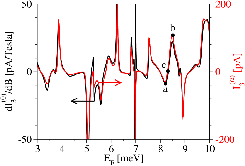
Figure 2: (Color online) Comparison of the spin current $I_{3}^{(\alpha)}(B=0)$ (red or gray line; right y axis) and the zero-field derivative $\partial_{B}I_{3}^{(0)}|_{B=0}$ of the charge current (black line; left y axis) measured at terminal 3, as a function of the Fermi energy $E_{F}$. The tags a-c refer to panels in Fig. 3.

We use material parameters corresponding to GaAs heterostructures, i.e. $m=0.067m_{e}$, with $m_{e}$ the free electron mass, $g=-0.44$, and we vary $E_{F}\in[3,10]$ meV. Leads 1 and 2 are 50 nm wide, corresponding to up to three open transport channels in the considered energy range. The terminal voltages are $V_{1}=-V_{2}=50$ $\mu$V and $V_{3}$ is set such that $I_{3}^{(0)}(B=0)=0$. For the QPC we set $\hbar\omega\approx 0.18$ meV, corresponding to a spin resolution at $B\approx 6$ T, and we take it to be 1.2 $\mu$m long to obtain numerically sharp conductance steps. The temperature effects on the QPC transmission can be neglected if $k_{B}T\ll\hbar\omega$, which is fulfilled at sub-Kelvin temperatures. Our numerics limits the dot linear size to about 200 nm, and accordingly we scale down the spin-orbit length to $l_{\rm br}=100$ nm, about an order of magnitude stronger than is typical for GaAs heterostructures, where 10 times larger dots have broken spin rotational symmetry Folk et al. (2001). As an unwanted numerical artifact the QPC itself affects the spin, being much longer than the spin-orbit length. These effects are minimal in the presence of only one type of spin-orbit interaction and we choose the Bychkov-Rashba one. We checked, but do not show that our numerical results are qualitatively unchanged for other types of spin-orbit interaction.

We first illustrate the validity of Eq. (1) in Fig. 2. We see that the zero-field derivative of the charge current in lead 3 faithfully follows the spin current, despite large fluctuations of the latter as the Fermi energy is varied. The two quantities are almost perfectly correlated, except close to 7 meV, where the number of channels in leads 1 and 2 artificially jumps from 2 to 3 due to the way we model the leads. This is a numerical artifact. We numerically calculated the current derivative as $\partial_{B}I_{3}^{(0)}|_{B=0}=[I_{3}^{(0)}(B/2)-I_{3}^{(0)}(-B/2)]/B$ with $B=10^{-3}$ T. Experimentally, however, the magnetic field must be large enough that the current change is measurable, but still small enough that (i) it does not generate mesoscopic fluctuations of the transmission coefficient $\tau_{3i}^{\sigma\sigma^{\prime}}(B)$ [see Eq. (4)], (ii) it does not polarize the QPC, since this would make $I_{3}^{(\alpha)}$ saturate, and (iii) it does not freeze spin-orbit interaction inside the dot. The upper bound on $B$ comes from (i) since, according to Ref. Zumbühl et al. (2004), $\tau_{3i}^{\sigma\sigma^{\prime}}(B)$ decorrelates at a field of about 1 T for a ballistic micron sized GaAs dot, while bounds on (ii) and (iii) are at $B\gtrsim 5$ T or more. Limiting ourselves to fields of 0.5 T, we estimate from Fig. 2 that a current sensitivity of about 10 pA is sufficient for spin-to-charge conversion of typical spin currents in ballistic lateral dots in GaAs.

Figure 3: (Color online) Spin (red or gray lines) and charge (black lines) currents in terminal 3 as a function of the in-plane magnetic field $B$. (a)-(c) Spin-orbit coupled dots corresponding to the labeled data points in Fig. 2. Dotted lines show the slope of the charge current at $B=0$. (d) Dot without spin-orbit interaction (solid lines) and dot with voltages $V_{1}=V_{2}=V/2=-V_{3}$ (dashed lines).

We finally focus on the parameter sets for the data points labeled “a”, “b” and “c” in Fig. 2, corresponding to negative, positive, and zero spin current at $B=0$ respectively. The first three panels of Fig. 3 show the magnetic-field dependence of $I_{3}^{(0)}$ and $I_{3}^{(\alpha)}$ in these three instances. The data clearly illustrate that the sign and magnitude of the spin current at $B=0$ is reflected in the slope of the electric current. We furthermore see that the electric current is linear up to magnetic field of 1-2 T, up to where, therefore, the zero-field derivative of the electric current can still be extracted. Figure 3(d) additionally shows that the current is exactly even in $B$ in the absence of spin current. This would happen in the absence of spin-orbit interaction, or if the leads 1 and 2 are set to the same voltage, biased with respect to the single-channel lead 3. The latter case provides a simple check of our method, as in this setup the spin current is forbidden Zhai and Xu (2005); Kiselev and Kim (2005).

While we focused on a QPC set to a maximal sensitivity, $\Gamma|_{B=0}=1/2$, our theory remains valid away from there [or for a QPC with a transmission different from the one in Eq. (5)] provided one substitutes $\pi\mu/\hbar\omega\to\partial_{B}{\rm ln}\Gamma|_{B=0}$ in Eq. (1). Also, we considered $V_{3}$ fixed while changing B. An alternative is to set it such that $I_{3}^{(0)}(B)=0$. Then Eq. (1) is replaced by

$$I_{3}^{(\alpha)}(B=0)\simeq\frac{\hbar\omega}{\pi\mu}\frac{e^{2}}{h}[2-\mathcal{T}_{33}^{(0)}]\partial_{B}V_{3}(B)|_{B=0}\,.$$ (11)

The spin current can thus also be extracted from a voltage measurement, however, this additionally requires a measurement of $\mathcal{T}_{33}^{(0)}$.

Conclusions. Our theoretical and numerical investigations show how mesoscopic spin currents can be converted into electric signals by measuring the magnetic-field response of the electric current through a QPC. Qualitatively, the presence or absence of a spin current is directly reflected in the symmetry of the electric current through the QPC. We moreover demonstrated that, beyond emphasizing the presence of a spin current, our measurement scheme renders the magnitude of the current quantitatively accessible, since the proportionality coefficient in Eq. (1) can be experimentally extracted from the transconductance of the QPC at a large Zeeman field. We estimate that typical spin currents flowing in GaAs quantum dots with broken spin rotational symmetry have a measurable electric signature at magnetic fields that are low enough that the targeted spin current is not altered by the measurement process. Finally, we stress that our scheme works independently of the source of spin current.

Acknowledgements. We would like to thank Brian LeRoy for valuable discussions. This work has been supported by the NSF under Grant No. DMR-0706319.

References

- Fabian et al. (2007) J. Fabian, A. Matos-Abiague, C. Ertler, P. Stano, and I. Žutić, Acta Phys. Slov. 57, 565 (2007), arXiv:0711.1461.
- Jedema et al. (2002) F. J. Jedema, H. B. Heersche, A. T. Filip, J. J. A. Baselmans, and B. J. van Wees, Nature 416, 713 (2002).
- Thomas et al. (1996) K. J. Thomas, et al., Phys. Rev. Lett. 77, 135 (1996).
- Elzerman et al. (2004) J. M. Elzerman, et al., Nature 430, 431 (2004).
- Shorubalko et al. (2007) I. Shorubalko, et al., Nanotech. 18, 044014 (2007).
- Amasha et al. (2008) S. Amasha, et al., Phys. Rev. B 78, 041306(R) (2008).
- Potok et al. (2003) R. M. Potok, et al., Phys. Rev. Lett. 91, 016802 (2003).
- Potok et al. (2002) R. M. Potok, J. A. Folk, C. M. Marcus, and V. Umansky, Phys. Rev. Lett. 89, 266602 (2002).
- Koop et al. (2008) E. J. Koop, B. J. van Wees, D. Reuter, A. D. Wieck, and C. H. van der Wal, Phys. Rev. Lett. 101, 056602 (2008).
- Frolov et al. (2009) S. M. Frolov, A. Venkatesan, W. Yu, J. A. Folk, and W. Wegscheider, Phys. Rev. Lett. 102, 116802 (2009).
- Kiselev and Kim (2001) A. A. Kiselev and K. W. Kim, Appl. Phys. Lett. 78, 775 (2001).
- Kiselev and Kim (2003) A. A. Kiselev and K. W. Kim, J. Appl. Phys. 94, 4001 (2003).
- Bardarson et al. (2007) J. H. Bardarson, İ. Adagideli, and Ph. Jacquod, Phys. Rev. Lett. 98, 196601 (2007).
- Nazarov (2007) Y. V. Nazarov, New J. Phys. 9, 352 (2007).
- Krich and Halperin (2008) J. J. Krich and B. I. Halperin, Phys. Rev. B 78, 035338 (2008).
- Adagideli et al. (2010) İ. Adagideli, et al., Phys. Rev. Lett. 105, 246807 (2010).
- Ren et al. (2006) W. Ren, Z. Qiao, J. Wang, Q. Sun, and H. Guo, Phys. Rev. Lett. 97, 066603 (2006).
- Zumbühl et al. (2004) D. M. Zumbühl, et al., Phys. Rev. B 69, 121305(R) (2004).
- Onsager (1931) L. Onsager, Phys. Rev. 38, 2265 (1931).
- Büttiker (1986) M. Büttiker, Phys. Rev. Lett. 57, 1761 (1986).
- Grbić et al. (2007) B. Grbić, et al., Phys. Rev. Lett. 99, 176803 (2007).
- Büttiker (1990) M. Büttiker, Phys. Rev. B 41, 7906 (1990).
- Adagideli et al. (2006) İ. Adagideli, G. E. W. Bauer, and B. I. Halperin, Phys. Rev. Lett. 97, 256601 (2006).
- Rashba (2003) E. I. Rashba, Phys. Rev. B 68, 241315 (2003).
- Folk et al. (2001) J. A. Folk, et al., Phys. Rev. Lett. 86, 2102 (2001).
- Zhai and Xu (2005) F. Zhai and H. Q. Xu, Phys. Rev. Lett. 94, 246601 (2005).
- Kiselev and Kim (2005) A. A. Kiselev and K. W. Kim, Phys. Rev. B 71, 153315 (2005).