On the Lipschitz constant of the RSK correspondence

Abstract

We view the RSK correspondence as associating to each permutation $\pi\in S_{n}$ a Young diagram $\lambda=\lambda(\pi)$, i.e. a partition of $n$. Suppose now that $\pi$ is left-multiplied by $t$ transpositions, what is the largest number of cells in $\lambda$ that can change as a result? It is natural refer to this question as the search for the Lipschitz constant of the RSK correspondence.

We show upper bounds on this Lipschitz constant as a function of $t$. For $t=1$, we give a construction of permutations that achieve this bound exactly. For larger $t$ we construct permutations which come close to matching the upper bound that we prove.

1 Introduction

The Robinson-Schensted-Knuth (RSK) correspondence [10, 11, 7] maps an arbitrary permutation $\pi\in S_{n}$ bijectively to an ordered pair of Young tableaux of the same shape $\lambda=\lambda(\pi)$. How much can $\lambda(\pi)$ change as we mildly vary $\pi$? For example, if we left-multiply $\pi$ by $t$ transpositions, to what extent can $\lambda$ change? We begin with the case when $t=1$ and show that the resulting Young diagram can differ from $\lambda$ on at most $\sqrt{n/2}$ cells. We show that this bound is tight by giving explicit constructions of permutations $\pi$ for which this bound is attained where the diagrams differ in at least $(1-o(1))\sqrt{n/2}$ cells. We then turn to consider the same question for larger $t$ and show that the corresponding diagram changes in at most $O(\sqrt{nt\ln t})$ cells. The best constructions we know nearly match this bound and yield, e.g., $(1-o(1))\sqrt{nt/2}$ changes for $t=o(n)$.

The outline of this paper is as follows. In the remainder of this section we recall some definitions and properties of Young tableaux and the RSK correspondence. In Section 2 we prove upper bounds on the Lipschitz constant when $t=1$ and show a matching construction. In Section 3 we give upper bounds and extend our constructions for the case of general $t$. We conclude with some directions for further research in Section 4.

1.1 Notation and Preliminaries

We recall some definitions and background on Young Tableaux and the RSK algorithm here. For more detailed expositions refer to [4, 9] or [12].

Let $n\in\mathbb{N}$ be a positive integer. A vector $\lambda=(\lambda_{1},\lambda_{2},\dots)$ of positive integers is a partition of $n$ (denoted by $\lambda\vdash n$) if

$$\lambda_{1}\geq\lambda_{2}\geq\dots>0\ \mathrm{and}\ \sum_{i}\lambda_{i}=n.$$

The Young diagram (or diagram) of a partition $\lambda$ is a left-justified array of cells with $\lambda_{i}$ cells in the $i$-th row for each $i\geq 1$. For example, the diagram of the partition $(5,5,3,2)$ is

$$\Young&\cr\cr\cr\cr$$

The cell in the $i$-th row and $j$-th column is referenced by its coordinate $(i,j)$. Thus $(1,1)$ is the top leftmost cell of the diagram.

The conjugate of a partition $\lambda$, denoted by $\lambda^{\prime}$ is the partition whose diagram is the transpose of the diagram of $\lambda$.

A standard Young tableau (SYT or tableau) of size $n$ with entries from $[n]$ is a diagram whose cells are filled with the elements of $[n]$ in such a way that the entries are strictly increasing from left to right along a row as well as from top to bottom down a column. The shape of a tableau $T$, denoted $sh(T)$ is the partition corresponding to the diagram of $T$. For example,

$$\Young 1&247\cr 36\cr 5\cr$$

is a tableau of size $7$ of shape $(4,2,1)$. Note that the elements in the cells of a SYT are distinct integers. Let $\mathcal{T}_{n}$ denote the set of SYT of size $n$.

1.2 The Robinson-Schensted-Knuth (RSK) Correspondence

The RSK correspondence discovered by Robinson [10], Schensted [11] and further extended by Knuth [7] is a bijection between the set of permutations $S_{n}$ and pairs of tableau of size $n$ of the same shape. This bijection is intimately related to the representation theory of the symmetric group [6, 3], the theory of symmetric functions [12, Chapter 7], and the theory of partitions [1].

The bijection can be defined through a row-insertion algorithm first defined by Schensted [11] in order to study the longest increasing subsequence of a permutation. Suppose that we have a tableau $T$. The row-insertion procedure below inserts a positive integer $x$ that is distinct from all entries of $T$, into $T$ and results in a tableau denoted by $T\leftarrow x$.

1. Let $y$ smallest number larger than $x$ in the first row of $T$. Replace the cell containing $y$ with $x$. If there is no such $y$, add a cell containing $x$ to the end of the row.

2. If $y$ was removed from the first row, attempt to insert it into the next row by the same procedure as above. If there is no row to add $y$ to, create a new row with a cell containing $y$.

3. Repeat this procedure on successive rows until either a number is added to the end of a row or added in a new row at the bottom.

The RSK correspondence from $S_{n}$ to $\{(P,Q)\in\mathcal{T}_{n}\times\mathcal{T}_{n}\ :\ sh(P)=sh(Q)\}$ can now be defined as follows. Let $\pi\in S_{n}$ and let $\pi_{i}$ denote the element of $[n]$ in position $i$ in $\pi$. Let $P_{1}$ be the tableau with a single cell containing $\pi_{1}$. Let $P_{j}=P_{j-1}\leftarrow\pi_{j}$ for all $1<j\leq n$ and set $P=P_{n}$. The tableau $Q$ is defined recursively in terms of tableaux $Q_{i}$ of size $i$ as follows. Let $Q_{1}$ be the tableau with one cell containing the integer $1$. The equality of shapes $sh(Q_{i})=sh(P_{i})$ is maintained throughout the process. The cell of $Q_{i}$ containing $i$ is the (unique) cell of $P_{i}$ that does not belong to $P_{i-1}$. The remaining cells of $Q_{i}$ are identical to those of $Q_{i-1}$. Finally, set $Q=Q_{n}$. We refer to $P$ as the insertion tableau and $Q$ is the recording tableau.

Let $\pi\in S_{n}$ and let $(P,Q)$ be the corresponding tableaux under the RSK correspondence. The shape of $\pi$ is $sh(P)=sh(Q)$ and will be denoted by $\lambda=\lambda(\pi)$. The RSK correspondence has numerous interesting properties (see [4, 9, 8] or [12]). Some that will be useful in particular are as follows.

Proposition 1.1.

Let $\lambda=\lambda(\pi)$. Then the diagram corresponding to $\pi^{R}$, the reversal of $\pi$, is $\lambda^{\prime}$, the conjugate of $\lambda$.

Proposition 1.2.

Let $(P,Q)$ be the tableaux corresponding to a permutation $\pi$ under the RSK correspondence. Then the tableaux corresponding to the inverse permutation $\pi^{-1}$ are $(Q,P)$. Thus the shape remains invariant upon inversion, i.e., $\lambda(\pi^{-1})=\lambda(\pi)$.

1.3 Motivation and Related Work

In view of the important role of the RSK correspondence, it is natural to investigate various aspects of it. Thus Fomin’s appendix in [12, Chapter 7] starts with the following two motivating questions:

1. Given a partition $\lambda$, characterize those permutations $\pi$ for which $\lambda(\pi)=\lambda$.

2. Given a tableau $P$, characterize the permutations $\pi$ which have $P$ as their insertion tableau.

We consider an approximate version of such questions and ask to what extent $\lambda$ changes as $\pi$ changes slightly. Question (1) is answered by the following theorem of Greene.

Theorem 1.3 (Greene [5]).

Let $\pi$ be a permutation, and suppose that the largest cardinality of the union of $j$ increasing subsequences in $\pi$ is $\mu_{j}$, then $\lambda(\pi)=\lambda_{1},\dots,\lambda_{k}$, where $\lambda_{1}=\mu_{1}$ and $\lambda_{j}=\mu_{j}-\mu_{j-1}$ for all $j\geq 2$.

In his study of the RSK correspondence, Knuth discovered certain equivalence relations that are key to the solution of Question (2) above. Two permutations are Knuth equivalent if one can be obtained from the other by certain restricted sequences of adjacent transpositions. Knuth equivalent permutations are the equivalency classes of permutations that have the same insertion tableau. For more on the subject, see [12].

In order to make our question concrete, we need to specify two measures of distance: One between permutations and the other between diagrams. A natural metric on permutations is left-multiplication by adjacent transpositions. An adjacent transposition is a permutation of the form $(i,i+1)$. Left-multiplying $\pi$ by an adjacent transposition is denoted by $(i,i+1)\circ\pi$ and means that first, the permutation $\pi$ is applied and then the transposition. We denote the least number of adjacent transpositions that transform the permutation $\pi$ to $\tau$ by $d(\pi,\tau)$. Recall that $d(\cdot,\cdot)$ is the graph metric in the Cayley graph of $S_{n}$ w.r.t. the generating set of adjacent transpositions $(1,2),(2,3),\dots,(n,n-1)$. We will say that two permutations $\pi$ and $\tau$ are at distance $t$ if $d(\pi,\tau)=t$. If $\lambda$ and $\mu$ are two diagrams, define their distance to be

$$\Delta=\Delta(\lambda,\mu):=\frac{1}{2}\sum_{i=1}^{n}|\lambda_{i}-\mu_{i}|.$$

Let $\pi$ and $\tau$ be any two permutations. We are interested in the Lipschitz constant of this mapping, i.e.,

$$L(n,t):=\max\frac{\Delta(\lambda(\pi),\lambda(\tau))}{d(\pi,\tau)}$$

where the maximum is over all $\pi,\tau\in S_{n}$ with $d(\pi,\tau)=t$.

The choice of left-multiplication above is in fact without loss of generality. By Proposition 1.2 the shape of a permutation and its inverse under the RSK correspondence are the same. Our results thus all follow immediately for right-multiplication since $\tau=(i,i+1)\circ\pi$ is equivalent to $\pi^{-1}=\tau^{-1}\circ(i,i+1)$.

In general, although $d$ and $\Delta$ are natural metrics to study for permutations and diagrams respectively, the same question can be asked for other metrics. We discuss the extension of our results to other metrics on permutations in Section 4.

2 Exact Bounds on the Lipschitz Constant for a Single Transposition.

In this section we will show upper bounds on the Lipschitz constant when the number of transpositions $t=1$. We also give a construction of a family of permutations which achieve this bound asymptotically.

2.1 Upper Bounds

The first step of the proof is to show that left-multiplying a permutation by a transposition can result in only a bounded number of cells being different in each row of the diagram.

Proposition 2.1.

Let $\pi,\tau\in S_{n}$ and let $\lambda,\mu$ be the respective diagrams. Suppose that $\tau=(i,i+1)\circ\pi$, and $\pi_{i}<\pi_{i+1}$. Then,

$$\forall\ 1\leq j\leq n,\ \ \ \ \sum_{i=1}^{j}\mu_{i}\leq\sum_{i=1}^{j}\lambda_{i}\leq\sum_{i=1}^{j}\mu_{i}+1$$ (1)

Proof.

Suppose that the largest cardinality of the union of $j$ increasing subsequences in $\pi$ is $\ell$. Suppose there is a subsequence which includes the pair that is being transposed in $\pi$. By deleting one of the elements of the pair we obtain a set of $j$ increasing subsequences of $\tau$ whose cardinality is at least $\ell-1$. If there is no such subsequence, then the same $j$ subsequences are also increasing in $\tau$. By Greene’s Theorem 1.3 this implies $\sum_{i=1}^{j}\lambda_{i}\leq\sum_{i=1}^{j}\mu_{i}+1.$

For the lower bound, consider the largest cardinality of the union of $j$ increasing sequences in $\tau$. No subsequence in this union can contain both of the elements involved in the transposition. Since the pair involved in the transposition have no other elements between them in both $\pi$ and $\tau$ the subsequences are also increasing in $\pi$. We conclude in the same way that $\sum_{i=1}^{j}\mu_{i}\leq\sum_{i=1}^{j}\lambda_{i}.$ ∎

Figure 1 will be useful in the following discussion. It depicts the union of two diagrams $\lambda$ and $\mu$, which is also a Young diagram. The symmetric difference consists of the cells marked by a dot. The remaining set of cells of the diagram labeled $W$ is the intersection of $\lambda$ and $\mu$ and this is a Young diagram as well.

Corollary 2.2.

Let $\pi,\tau\in S_{n}$ where $d(\pi,\tau)=1$ and let $\lambda,\mu$ be the corresponding diagrams. Then at most one cell in each row and each column of the union of $\lambda$ and $\mu$ can be in the symmetric difference.

Proof.

To see this for a row $r$, consider inequality (1) for $j=r$ and for $j=r-1$ and take their difference. A similar argument applied to the reversed permutations implies the claim for columns. (see Proposition 1.1). ∎

Theorem 2.3.

Let $\pi$ and $\tau$ be permutations in $\mathcal{S}_{n}$ with respective Young diagrams $\lambda$ and $\mu$, and suppose that $d(\pi,\tau)=1$. Then

$$\Delta=\Delta(\lambda,\mu)\leq\sqrt{\frac{n}{2}}.$$

Figure 1: The union of $\lambda$ and $\mu$ with cells of the symmetric difference marked.

Proof.

As shown in Figure 1, let $(i,j)$ and $(i^{\prime},j^{\prime})$ be the coordinates of two distinct cells in the symmetric difference. By Corollary 2.2, $i\neq i^{\prime}$ and $j\neq j^{\prime}$, and $(\min(i,i^{\prime}),\min(j.j^{\prime}))\in W$. This gives a 1:1 map from unordered pairs of cells in the symmetric difference into $W$. Therefore,

$${2\Delta\choose 2}\leq n-\Delta$$

implying the required bound

$$\Delta\leq\sqrt{\frac{n}{2}}.\qed$$

2.2 Construction

In this section we construct pairs of permutations in $S_{n}$ which differ by a single transposition whose corresponding Young diagrams differ by at least $(1-o(1))\sqrt{n/2}$ cells, matching the upper bound in Theorem 3.2 asymptotically. The following lemma characterizes the shape of a permutation by the cardinalities of increasing and decreasing subsequences.

Lemma 2.4.

Let $\pi\in S_{n}$ be a permutation whose elements can be decomposed in the following two ways: (i) into increasing subsequences of cardinalities $\lambda_{1},\lambda_{2},\dots$, and (ii) into decreasing subsequences of cardinalities $\lambda_{1}^{\prime},\lambda_{2}^{\prime},\dots$, where the partitions $\lambda$ and $\lambda^{\prime}$ are conjugate. Then $\lambda=\lambda(\pi)$.

Proof.

By Greene’s Theorem 1.3 it suffices to show that for each $r$, the largest cardinality of the union of $r$ increasing sequences in $\pi$ is $\sum_{i\leq r}\lambda_{i}$. By assumption we know it is at least this number and we need to show the opposite inequality. Namely, that if $s_{1},\dots,s_{j}$ is a collection of disjoint increasing sequences in $\pi$, $\sum_{i=1}^{r}|s_{i}|\leq\sum_{i\leq r}\lambda_{i}$.

By assumption, there is a decomposition $d_{1},d_{2}\dots$ of $\pi$ into disjoint decreasing subsequences of cardinalities $\lambda_{1}^{\prime},\lambda_{2}^{\prime},\dots$. But each $s_{i}$ and $d_{j}$ can have at most one element in common, so that

$$\sum_{i=1}^{r}|s_{i}|=\sum_{r\geq i\geq 1,~{}j}|s_{i}\cap d_{j}|\leq\sum_{j}\min\{|d_{j}|,r\}=\sum_{j}\min\{\lambda_{j}^{\prime},r\}=\sum_{i=1}^{r}\lambda_{i}$$

where the last equality follows because the partitions $\lambda_{1},\lambda_{2},\dots$ and $\lambda_{1}^{\prime},\lambda_{2}^{\prime},\dots$ are conjugate. ∎

Theorem 2.5.

For every $n$ there are permutations $\pi,\tau\in S_{n}$ with $d(\pi,\tau)=1$ and respective shapes $\lambda,\mu$ such that $\Delta(\lambda,\mu)\geq(1-o(1))\sqrt{n/2}$.

Proof.

Our proof says, in fact, a little more than what is stated. Namely for $n=(k+1)^{2}/2$ with $k$ an odd integer, we will construct two permutations $\pi$ and $\tau$ of shapes $\lambda=(k+1,k-1,k-1,\dots,2,2)$ and $\mu=(k,k,k-2,k-2,\dots,1,1)$ which differ by exactly one cell in each row and column, giving $\Delta=\sqrt{n/2}$. Thus it can be verified that together with Theorem 2.3 this gives a complete answer to our question for $n$ of this form. For other values of $n$ we get the result by padding this basic construction. In the discussion that follows we decompose these permutations into monotone subsequences. The decompositions we exhibit are not necessarily unique, but for our purpose any decomposition suffices.

The construction can, perhaps, be best understood by observing alongside with the general discussion a concrete special case. So we intersperse our general constructions with an illustration that shows how things work for $n=18$ ($k=5$). We start by dividing the elements of $[n]$ into three categories according to their magnitude. The “small” elements are those in the interval $[1,n/2-\frac{k+1}{2}]$. The next $k+1$ elements, i.e., interval $[n/2-\frac{k-1}{2},n/2+\frac{k+1}{2}]$ are “intermediate” and members of the interval $[n/2+\frac{k+3}{2},n]$ are “big”.

We further subdivide the big elements (in order) into blocks $b_{1},\dots,b_{(k-1)/2}$. The small elements are split (in order) into blocks $s_{(k-1)/2},\ldots,s_{1}$. Both $s_{i}$ and $b_{i}$ have cardinality $2i$.

$$\begin{array}[]{ccc}s_{2}\ \ \ \ \ \ \ \ s_{1}&&b_{1}\ \ \ \ \ \ \ \ \ \ \ b_{2}\\ \underbrace{(1\ 2\ 3\ 4)\ (5\ 6)}&\underbrace{7\ 8\ 9\ 10\ 11\ 12}&\underbrace{(13\ 14)\ (15\ 16\ 17\ 18)}\\ \mathrm{small}&\mathrm{intermediate}&\mathrm{big}\\ \end{array}$$

The permutation $\pi$ is constructed by spreading out the intermediate elements with $n/2$ and $n/2+1$ remaining fixed points (see below). The blocks of big elements are then inserted in the order $b_{(k-1)/2},\dots,b_{1}$ in the spaces between the smaller intermediate elements while the blocks of small elements are inserted in the order $s_{1},\dots,s_{(k-1)/2}$ in the spaces between the larger intermediate elements. To obtain $\tau$ we apply the transposition $(n/2,n/2+1)$ to $\pi$. The permutations are defined in this manner with a view to decomposing them into increasing and decreasing sequences of desired cardinalities.

$$\pi=7(15\ 16\ 17\ 18)\ 8\ (13\ 14)\ \underline{9\ 10}\ (5\ 6)\ 11\ (1\ 2\ 3\ 4)\ 12$$

$$\tau=7(15\ 16\ 17\ 18)\ 8\ (13\ 14)\ \underline{10\ 9}\ (5\ 6)\ 11\ (1\ 2\ 3\ 4)\ 12$$

From the construction we claim that $\pi$ and $\tau$ can be decomposed into a disjoint union of increasing subsequences of cardinalities $(k+1,k-1,k-1,\dots,2,2)$ and $(k,k,k-2,k-2,\dots,1,1)$ respectively. For $\pi$ the increasing sequences consist of (i) The intermediate elements, which in our example is $7,8,9,10,11,12$, (ii) The blocks of small elements, i.e., $1,2,3,4$ and $5,6$ and (iii) The blocks of big elements, i.e., $15,16,17,18$ and $13,14$.

The permutation $\tau$ can be decomposed into the increasing subsequences of the following three types: (i) An intermediate element and the block of big elements following it, which in the example are $7,15,16,17,18$ and $8,13,14$, (ii) A block of small elements and the following intermediate element, i.e., $5,6,11$ and $1,2,3,4,12$ and (iii) The two subsequences of length one consisting of one of the two middle intermediate elements, i.e. $10$ and $9$.

The proof that $\pi$ and $\tau$ have the shapes $\lambda=(k+1,k-1,k-1,\dots,2,2)$ and $\mu=(k,k,k-2,k-2,\dots,1,1)$ respectively uses Lemma 2.4. It is enough to decompose $\pi$ and $\tau$ into a union of decreasing sequences whose cardinalities are given by the respective conjugate sequences. Note that as it happens, the shapes $\lambda$ and $\mu$ are conjugates.

We assign the elements of $\pi$ to decreasing subsequences $d_{1},\dots,d_{k+1}$ of cardinalities $k,k,\dots,1,1$. as follows. Since the $d_{i}$ are subsequences, elements in them appear in the same order as in the permutation. Secondly, the assignment is made so that each subsequence has exactly one of the intermediate elements, and it appears after any of the big elements and before any of the small elements. (There is more than one way to do this.) We first see how this is done in the example.

We first construct $d_{1}$ and $d_{2}$ which are both decreasing sequences of length $5$. The largest elements in the blocks $b_{i}$, the largest elements in the blocks $s_{i}$ and one of the middle intermediate elements are assigned to $d_{1}$. Then we choose $d_{2}$ similarly from among the remaining elements.

$$d_{1}\ :\ 7(15\ 16\ 17\ \framebox{18})\ 8\ (13\ \framebox{14})\ \framebox{9}\ 10\ (5\ \framebox{6})\ 11\ (1\ 2\ 3\ \framebox{4})\ 12$$

$$d_{2}\ :\ 7(15\ 16\ \framebox{17}\ \cancel{18})\ 8\ (\framebox{13}\ \cancel{14})\ \cancel{9}\ \framebox{10}\ (\framebox{5}\ \cancel{6})\ 11\ (1\ 2\ \framebox{3}\ \cancel{4})\ 12$$

The remaining elements can be seen to have the same structure recursively (the remaining elements appear in the same relative order as would the elements of the permutation for $n=8$), where the brackets indicate blocks of big and small elements as before.

$$7(15\ 16)\ 8\ 11\ (1\ 2)\ 12$$

To assign elements to $d_{3}$ and $d_{4}$, we want to continue with the strategy of choosing the largest elements that remain in the blocks. Note that since the big elements 13 and 14 have been assigned, there are no big elements that follow the element 8, and it now becomes “available”. Thus $d_{3}$ and $d_{4}$ are constructed by assigning the largest elements that remain in the small and big blocks and one of the remaining intermediate elements in the middle of the blocks.

$$d_{3}\ :\ 7(15\ \ \framebox{16}\ \cancel{17}\ \cancel{18}\ )\ \framebox{8}\ (\cancel{13}\ \cancel{14})\ \cancel{9}\ \cancel{10}\ (\cancel{5}\ \cancel{6})\ \ 11\ \ (\ 1\ \ \framebox{2}\ \cancel{3}\ \cancel{4})\ 12$$

$$d_{4}\ :\ 7(\framebox{15}\ \ \cancel{16}\ \ \cancel{17}\ \cancel{18})\ \ \cancel{8}\ \ (\cancel{13}\ \cancel{14})\ \cancel{9}\ \cancel{10}\ (\cancel{5}\ \cancel{6})\ \framebox{11}\ (\framebox{1}\ \ \cancel{2}\ \ \cancel{3}\ \cancel{4})\ 12$$

Proceeding the same way, we obtain the subsequences: $d_{1}=18,14,9,6,4$, $d_{2}=17,13,10,5,3$, $d_{3}=16,8,2$, $d_{4}=15,11,1$, $d_{5}=7$, $d_{6}=12$. In general, the assignment is done as follows.

• The $i$-th largest element in each block of big elements, is assigned to the subsequence $d_{i}$.

• The $i$-th largest element in each block of small elements, is assigned to the subsequence $d_{i}$.

• For the intermediate elements, assign the lower $(k+1)/2$ elements to the subsequences $d_{k},d_{k-2},\dots,d_{1}$ (in that order) and the top $(k+1)/2$ elements to $d_{2},\dots,d_{k-1},d_{k+1}$ (in that order).

Clearly, this is a decomposition of $[n]$ with exactly $k-2\lfloor(i-1)/2\rfloor$ elements in $d_{i}$. It remains to show that each $d_{i}$ is a decreasing subsequence. By the construction of the permutation, the big and small elements in $d_{i}$ form a decreasing subsequence since each of them is from a different block. Secondly, the intermediate element in $d_{i}$ appears after all the big elements and before any of the the small ones.

Similarly, for the permutation $\tau$, we define the decreasing subsequences $f_{1},\dots,f_{k}$ of cardinalities $k+1,k-1,k-1,\dots,2,2$, where $|f_{i}|=k+1-2\lfloor i/2\rfloor$. As before, the assignment is made so that each sequence but for one (which has the two middle intermediate elements) has at most one intermediate element, and at most one element from each of the small and the big blocks. In our example, we construct $f_{1}$, a subsequence of length $6$, by taking the largest element from each block and the two middle intermediate elements.

$$f_{1}\ :\ 7(15\ 16\ 17\ \framebox{18})\ 8\ (13\ \framebox{14})\ \framebox{10}\ \framebox{9}\ (5\ \framebox{6})\ 11\ (1\ 2\ 3\ \framebox{4})\ 12$$

Next, we choose $f_{2}$ and $f_{3}$ which are both subsequences of length $4$. At this point, we cannot continue to follow the strategy of assigning the largest elements from each block to $f_{2}$ (by choosing $17,13,5,3$) as in the next step we would fail to construct $f_{3}$ of length $4$. Instead, note that when only one element remains in a block of small elements, the intermediate element which follows that block has not yet been assigned and it does not follow any other small elements. Thus the strategy for $f_{2}$ is to assign to it the largest elements from all blocks except from $s_{1}$ in which only one element remains, and to assign the intermediate element following $s_{1}$ to $f_{2}$. To construct $f_{3}$, we take the largest remaining elements in all the blocks, and the intermediate element that precedes the block of big elements whose smallest element was assigned to $f_{2}$. Diagrammatically, we have:

$$f_{2}\ :\ 7(15\ \ 16\ \ \framebox{17}\ \cancel{18})\ \ 8\ \ (\framebox{13}\ \cancel{14})\ \cancel{10}\ \cancel{9}\ (\ 5\ \ \cancel{6})\ \framebox{11}\ (1\ \ 2\ \ \framebox{3}\ \cancel{4})\ 12$$

$$f_{3}\ :\ 7(15\ \framebox{16}\ \ \cancel{17}\ \ \cancel{18})\ \framebox{8}\ (\ \cancel{13}\ \ \cancel{14})\ \cancel{10}\ \cancel{9}\ (\framebox{5}\ \cancel{6})\ \ \cancel{11}\ \ (1\ \framebox{2}\ \ \cancel{3}\ \ \cancel{4})\ 12$$

Repeating the same arguments for the remaining elements, we obtain the following subsequences for the example: $f_{1}=18,14,10,9,6,4$, $f_{2}=17,13,11,3$, $f_{3}=16,8,5,2$, $f_{4}=15,12$, $f_{5}=7,1$. In general, the subsequences can be defined as follows.

• The $i$-th largest element in each block of big elements is assigned to $f_{i}$.

• The smallest element in a block of small elements $s_{j}$ is assigned to $f_{2j+1}$. Among the remaining elements, the $i$-th largest element goes to $f_{i}$.

• The lower $(k-1)/2$ of the intermediate elements go to $f_{k},f_{k-2},\dots,f_{3}$ (in that order). The top $(k-1)/2$ elements to $f_{2},\dots,f_{k-1}$ (in that order). The two middle intermediate elements are in $f_{1}$.

As before, the $f_{i}$ constitute a decomposition and they have the appropriate sizes. By construction, the big and small elements in any subsequence $f_{i}$ form a decreasing subsequence. Lastly, for $i\neq 1$ there is at most one intermediate element in $f_{i}$ and if one exists, it appears after all the big elements and before all the small ones. For $i=1$, the two intermediate elements appear consecutively in decreasing order, after all big elements and before all small ones. Thus, $\pi$ and $\tau$ have the claimed shapes and it follows that

$$\Delta=\frac{k+1}{2}=\sqrt{\frac{n}{2}}.$$

For $n$ not of the form $(k+1)^{2}/2$, we construct two permutations as follows. Let $n_{0}<n$ be the largest integer such that $n_{0}=(k+1)^{2}/2$ for odd $k$. The first $n_{0}$ elements of $\pi$ and $\tau$ are set according to the construction above on $n_{0}$ elements. The last $n-n_{0}$ elements of both $\pi$ and $\tau$ are $n_{0}+1,\dots,n$. Then, we have that

$$\Delta=\sqrt{\frac{n_{0}}{2}}\geq(1-o(1))\sqrt{\frac{n}{2}}.\qed$$

We have carried out computer simulations and found other pairs of permutations for which the bound holds with equality. Several mysteries remain here, a few of which we mention in Section 4.

3 Bounds on the Lipschitz Constant for $t>1$

In this section we show bounds on the Lipschitz constant for $t>1$. Extending the arguments from the previous section for both the upper and lower bound gives bounds that are tight up to constant factors for $t=O(1)$. In the latter half of this section we give a more complicated argument that yields an improved upper bound for general $t$.

3.1 A construction for permutations at linear distance $t$.

The construction for the case of one transposition can be extended to the case of more than one transposition as follows.

Theorem 3.1.

Let $t\leq n/2$. For every $n$ there are permutations $\pi,\tau\in S_{n}$ with $d(\pi,\tau)=t$ and respective shapes $\lambda,\mu$ such that $\Delta(\lambda,\mu)\geq(1-\sqrt{t/2n})\sqrt{nt/2}$.

Proof.

Let $k=\lfloor\sqrt{2n/t}-1\rfloor$, and $m=(k+1)^{2}/2$ so that $mt\leq n$. Divide the first $mt$ elements of $[n]$ into $t$ blocks of length $m$ each. To construct the permutations, in each block we permute the elements as in the construction for one transposition, and then concatenate the blocks with the remaining $n-mt$ elements following. Then, it is not difficult to see that the RSK algorithm on this pair of permutations will result in a shape with $t$ of the smaller Young diagrams corresponding to each block being pasted one after the other, with an additional $n-mt$ boxes in the top row of each diagram. Then, $\Delta=t\sqrt{m/2}\geq\sqrt{nt/2}(1-\sqrt{t/2n})$. Thus when $t=o(n)$, $\Delta\geq(1-o(1))\sqrt{nt/2}$. ∎

3.2 Upper Bounds

We start with an easy observation:

Theorem 3.2.

Let $\pi$ and $\tau$ be permutations in $\mathcal{S}_{n}$ such that $d(\pi,\tau)=t$. Let $\lambda$ and $\mu$ be the respective Young diagrams. Then

$$\Delta=\Delta(\lambda,\mu)\leq t\sqrt{\frac{n}{2}}.$$

Proof.

Since $d(\pi,\tau)=t$, there is a sequence of permutations $\pi=\sigma_{0},\sigma_{1},\dots,\sigma_{t}=\tau$ such that for each $0\leq i<t$, $\sigma_{i}$ and $\sigma_{i+1}$ differ by an adjacent transposition. The distance $\Delta(\cdot,\cdot)$ is a metric on diagrams and hence the bound follows by the triangle inequality from Theorem 2.3. ∎

We do not see how to appropriately adapt the bijective argument of Theorem 2.3. However, the following argument yields a near-optimal bound.

Theorem 3.3.

Let $\pi,\tau\in\mathcal{S}_{n}$ be such that $d(\pi,\tau)=t$. Let $\lambda,\mu$ be the corresponding diagrams. Then

$$\Delta(\lambda,\mu)\leq O(\sqrt{nt\ln t}).$$

We start by showing some preliminary results that will be useful in the proof. Suppose $\pi$ and $\tau$ are two permutations such that $d(\pi,\tau)=t$. Let $\pi=\sigma_{0},\sigma_{1},\dots,\\ \sigma_{t}=\tau$ be a sequence of permutations such that for each $0\leq i<t$, $\sigma_{i}$ and $\sigma_{i+1}$ differ by an adjacent transposition. Say that $s$ (resp. $r$) of the transpositions put the relevant pair in decreasing (resp. increasing) order, where $t=r+s$. Let $\lambda$ and $\mu$ be the diagrams corresponding to $\pi$ and $\tau$ respectively.

Lemma 3.4.

Let $\pi,\tau$ be as above. Then,

$$\forall\ 1\leq j\leq n,\ \ \ \ \sum_{i=1}^{j}\mu_{i}-r\leq\sum_{i=1}^{j}\lambda_{i}\leq\sum_{i=1}^{j}\mu_{i}+s$$ (2)

Proof.

For each pair $\sigma_{i},\sigma_{i+1}$ in the sequence of permutations $\pi=\sigma_{0},\sigma_{1},\dots,\sigma_{t}=\tau$, by Proposition 2.1 the inequality (1) holds for the diagrams corresponding to $\sigma_{i}$ and $\sigma_{i+1}$. The result is obtained by adding up all these inequalities. ∎

Figure 2: The union of $\lambda$ and $\mu$ and the symmetric difference split into blocks.

In Figure 2 we depict the union of two diagrams. Their intersection is labeled $W$ as before. We split the symmetric difference of the two diagrams into blocks. We say that $j$ indexes a $\lambda$-row if $\lambda_{j}>\mu_{j}$. A maximal interval of $\lambda$-rows determines a $\lambda$-pre-block. A maximal collection of consecutive $\lambda$-pre-blocks constitutes a $\lambda$-block. We likewise define $\mu$-blocks. Blocks are labeled $B_{i}$ as in the figure. The number of cells in a set $S$ will be denoted by $A(S)$. We use the following fact about the sizes of the blocks.

Proposition 3.5.

Let $d(\pi,\tau)=t$ with corresponding diagrams $\lambda$, $\mu$ and let $B$ be a block in the union of the diagrams, then $A(B)\leq t$.

Proof.

This bound is obtained from Lemma 3.4 as follows. Let $B$ reside in the set of rows $I$ of the diagram. Assuming it exists, let $i_{0}$ be the row just preceding $I$, and $i_{1}=\max I$. Then the bound is obtained by subtracting the inequality (2) corresponding to $j=i_{0}$ from the inequality corresponding to $j=i_{1}$, and using the fact that $r+s=t$. If there is no row $i_{0}$, then the bound is immediate from the inequality for $j=i_{1}$. ∎

The main step in the proof of Theorem 3.3 is the following lemma about two sequences of integers.

Lemma 3.6.

Let $k\geq 2$, $T\geq 3$ and let $a_{1},\dots,a_{k}$ and $b_{1},\dots,b_{k}$ be two sequences of positive integers. Denote $\Delta=\sum_{i=1}^{k}a_{i}b_{i}$ and $N=\sum_{1\leq i\leq j\leq k}a_{i}b_{j}.$ If

$$a_{1}=b_{k}=1\ \mathrm{and}\ \forall i,\ a_{i}b_{i}\leq T,$$

then

$$\Delta\leq\sqrt{32NT\ln T}.$$

This bound is tight up to constants.

We first show how to derive the theorem from Lemma 3.6.

Let $\lambda$ and $\mu$ be two diagrams of size $n$ (not necessarily corresponding to permutations at distance $t$). For the union of these diagrams, define the blocks of the symmetric difference $\{B_{i}\}$ and $W$ as before. Suppose that for each block $B$, $A(B)\leq t$. To prove Theorem 3.3, it is sufficient to show that for these diagrams,

$$\frac{1}{2}\sum_{i}A(B_{i})\leq O\left(\sqrt{t\ln t\left[A(W)+\frac{1}{2}\sum_{i}A(B_{i})\right]}\right)$$ (3)

With this formulation in mind, we can make the following assumptions about the pair of diagrams. The aim is to make a number of transformations and show that the pair of diagrams can be assumed to be of the form shown in Figure 6.

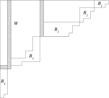
Figure 3: Rows and columns of $W$ that may be removed.

Reduction 1.

For any row $i$, $\lambda_{i}\neq\mu_{i}$ and similarly, for any column $j$, $\lambda_{j}^{\prime}\neq\mu_{j}^{\prime}$. If this is not the case (as in the shaded part of Figure 3), we delete such rows or columns from both $\lambda$ and $\mu$. Consequently, $A(W)$ decreases, whereas $\sum_{i}A(B_{i})$ remains unchanged. Thus, if the bound holds for the new pair of diagrams, it holds as well for the old pair.

Reduction 2.

In general, each block is a skew-diagram (the set theoretic difference of a diagram and another contained in it). However, as we show, we may assume it is a Young diagram. The dotted lines in Figure 4 mark the “shade” of a block in $W$ determined by its top row and leftmost column. If a block is not a (left-aligned) tableau, we can change it to one by removing the cells of $W$ in its shade and replacing it with a Young diagram of area $A(B)$ contained in the union of the block and its shade.

Figure 4: The top left corner of the block.

Figure 5: All blocks are Young diagrams.

Figure 6: A box of side lengths $a_{i}$ and $b_{i}$ bounds $B_{i}$.

This transformation decreases $A(W)$ and keeps the size of the block fixed. Secondly, we may assume that the transformation is done so that all rows of a block, with the possible exception of the last one have the same length. The result of such a transformation on the blocks $B_{2}$ and $B_{3}$ is shown in Figure 5.

Reduction 3.

We may assume that the topmost block $B_{1}$ has a single row. Otherwise, we can shift all the cells of $B_{1}$ to the first row without changing any $A(B_{i})$ or $A(W)$. We can then delete any rows of $W$ which are of the same length in $\lambda$ and $\mu$. By similar reasoning, we may assume that the bottommost block has a single column.

Thus, we may assume that the diagrams are as shown in Figure 6 and that the sizes of the blocks are bounded by $t$. As in the figure, let $a_{i}$ and $b_{i}$ denote the lengths of the vertical and horizontal sides of the rectangle which bounds the block $B_{i}$. Thus the area $A(W)$ can be written as a sum of areas of rectangles $a_{i}b_{j}$ whose sides are determined by the side lengths of pairs of blocks. Also note that by our construction of the blocks, $a_{i}b_{i}\leq 2t$.

To obtain the formulation of the lemma, suppose that we add cells to the last row of each block to complete it to a rectangle. Denote the modified blocks by $B^{\prime}$. Then for each block, $A(B^{\prime})\leq 2A(B)$. If we show the bound for these modified diagrams with a bound of $2t$ for each block, then the bound is implied for the original diagrams since the constants can be absorbed by the $O(\cdot)$. Formally, this follows from the following inequalities.

1. $\frac{1}{2}\sum_{i}A(B_{i})\leq\frac{1}{2}\sum_{i}A(B_{i}^{\prime})$

2. $A(W)+\frac{1}{2}\sum_{i}A(B_{i}^{\prime})\leq 2\left(A(W)+\frac{1}{2}\sum_{i}A(B_{i})\right)$

Thus Lemma 3.6 implies the bound (3) for a pair of diagrams as above and we have verified that to prove Theorem 3.3 it is sufficient to prove the lemma.

Proof of Lemma 3.6: We will minimize $N/\Delta^{2}$. For $k=2$, the lemma can be easily verified by calculation once we use the fact that $a_{1}=b_{2}=1$. Thus we will assume that $k\geq 3$. Consider the following relaxation of the minimization problem where the $a_{i},b_{j}$ are not necessarily integral.

$$\min\frac{N}{\Delta^{2}}=\frac{\displaystyle\sum_{1\leq i\leq j\leq k}a_{i}b_{j}}{\left(\displaystyle\sum_{i=1}^{k}a_{i}b_{i}\right)^{2}}$$

$$s.t.\ \ \ \ \ \ \ \ \ \ \ \ a_{1}=b_{k}=1$$

$$a_{i}b_{i}\leq T,\ 1\leq i\leq k$$

$$a_{i}\geq 1,\ 2\leq i\leq k$$

$$b_{i}\geq 1,\ 1\leq i\leq k-1$$

We will use the method of Lagrange multipliers (see Appendix A for a brief introduction) to obtain a lower bound on the value of the objective above at any local optimum. Since the problem is a relaxation of the discrete minimization problem, this also lower bounds the objective of the discrete problem. We obtain the following Lagrangian for the relaxation above.

$$\min\mathcal{L}= \frac{N}{\Delta^{2}}-\sum_{i=1}^{k}\lambda_{i}(a_{i}b_{i}-T)-\sum_{i=1}^{k}\mu_{i}(a_{i}-1)-\sum_{i=1}^{k}\nu_{i}(b_{i}-1)$$

The Karush-Kuhn-Tucker conditions yield the following necessary conditions for minimality.

$$\frac{\partial}{\partial a_{i}}\mathcal{L}=\frac{\partial}{\partial a_{i}}\frac{N}{\Delta^{2}}-\lambda_{i}b_{i}-\mu_{i}=0,\quad 1\leq i\leq k$$ (4)

$$\frac{\partial}{\partial b_{i}}\mathcal{L}=\frac{\partial}{\partial b_{i}}\frac{N}{\Delta^{2}}-\lambda_{i}a_{i}-\nu_{i}=0,\quad 1\leq i\leq k$$ (5)

$$\lambda_{i}\geq 0,~{}~{}\lambda_{i}(T-a_{i}b_{i})=0,\quad 1\leq i\leq k$$

$$\mu_{i}\geq 0,\quad\mu_{i}(a_{i}-1)=0,\quad 2\leq i\leq k$$

$$\nu_{i}\geq 0,\quad\nu_{i}(b_{i}-1)=0,\quad 1\leq i\leq k-1$$ (6)

From these conditions, we can show that at optimality either $a_{i}b_{i}=T$ or $1$. Suppose that for some $i$, $a_{i}b_{i}<T$. Note that by the conditions above, this implies $\lambda_{i}=0$. Now, if $a_{i}b_{i}\neq 1$, at least one of $a_{i}$ or $b_{i}$ is $>1$. Assume without loss of generality that $b_{i}>1$ (the argument in the other case is exactly the same). In this case $\nu_{i}=0$ by (6) . Hence from (5) above, we have

$$\frac{\partial}{\partial b_{i}}\frac{N}{\Delta^{2}}=0$$

and therefore, since $\Delta>0$

$$\Delta^{2}\frac{\partial N}{\partial b_{i}}=2\Delta N\frac{\partial\Delta}{\partial b_{i}}$$

$$\Rightarrow\quad \frac{\displaystyle\sum_{j=1}^{i}a_{j}}{2a_{i}}=\frac{N}{\Delta}$$ (7)

Now we show that it is possible to increase $b_{i}$ by a factor $(1+\varepsilon)$ for $\varepsilon>0$ so that $N/\Delta^{2}$ decreases and we can conclude that the solution is not optimal. This is allowed, at least for $\varepsilon>0$ small enough, since, by assumption $a_{i}b_{i}<T$. Let $N^{\prime}$ and $\Delta^{\prime}$ be the summations as defined before for the sequences where we replace $b_{i}$ by $b_{i}(1+\varepsilon)$.

$$\frac{N^{\prime}}{(\Delta^{\prime})^{2}}=\frac{N+b_{i}\varepsilon\displaystyle\sum_{j=1}^{i}a_{j}}{(\Delta+a_{i}b_{i}\varepsilon)^{2}}$$

To prove the claim $N^{\prime}/(\Delta^{\prime})^{2}<N/\Delta^{2}$, using the right hand side above, it is enough to show that

$$\Delta^{2}b_{i}\varepsilon\displaystyle\sum_{j=1}^{i}a_{j}<N\left(2\Delta a_{i}b_{i}\varepsilon+(a_{i}b_{i}\varepsilon)^{2}\right)$$

Or equivalently, dividing throughout by $2a_{i}b_{i}\varepsilon\Delta^{2}$, that

$$\frac{\displaystyle\sum_{j=1}^{i}a_{j}}{2a_{i}}<\frac{N}{\Delta}+\frac{Na_{i}b_{i}\varepsilon}{2\Delta^{2}}.$$

This inequality follows by (7). The left-hand term equals the first term on the right and $\varepsilon>0$.

The next step is to argue that it is enough to show the claimed bound assuming that the blocks are arranged in a specific manner (i.e., the sequences are of a certain form). In particular, the blocks of area $T$ are arranged such that $a_{i}$ is increasing and $b_{i}$ is decreasing. Secondly, the blocks of area $1$ occur after all blocks such that $a_{i}\leq b_{i}$ and before all blocks such that $a_{i}>b_{i}$. This can be argued by noticing that such an arrangement can be achieved by exchanging blocks which are out of order since $\Delta$ remains unchanged and $N$ does not increase. Thus a lower bound on $N/\Delta^{2}$ for the modified sequence is a lower bound on the corresponding quantity for the original sequence.

We next argue that, in fact, w.l.o.g. no block has area $1$. Recall that we wish to show

$$32T\ln TN-\Delta^{2}\geq 0.$$

We will show that if we add a single block of area $1$ then

$$32T\ln TN^{\prime}-\Delta^{\prime 2}\geq 32T\ln TN-\Delta^{2}$$ (8)

where $N^{\prime}$ and $\Delta^{\prime}$ are the modified values of $N$ and $\Delta$. This inequality above allows us to reduce the argument to the case when there are no blocks of area $1$. Let the shorter sequence have $k$ terms. Note that $\Delta^{\prime}=\Delta+1$ and the change in the number of cells $N^{\prime}-N$ is at least $\sum_{i=1}^{k}\min(a_{i},b_{i})$.

Recall that $k,T\geq 3$ and for $1\leq i\leq k$, $a_{i},b_{i}\geq 1$. Thus,

$$(\Delta^{\prime})^{2}-\Delta^{2}= \quad 2\Delta+1$$

$$\leq \quad 2kT+1$$

$$\leq \quad 32kT\ln T$$

$$\leq \quad 32T\ln T\sum_{i=1}^{k}\min(a_{i},b_{i})$$

$$= \quad 32T\ln T(N^{\prime}-N)$$

which implies the required inequality (8).

In the next step, we will make a further simplification to the picture. To summarize, we now know that we may optimize over sequences such that each block has size $T$, $a_{1}=b_{k}=1$, the sequence $a_{i}$ is non-decreasing and $b_{i}$ is non-increasing. The claim is that the optimal solution is of the form where there is some $i$ such that $a_{i}>1$ and $b_{i}>1$. If not, then it can be checked that $\Delta=\sqrt{8NT}$ and the claimed bound holds.

We relabel the sequences $a_{-\ell_{1}},\dots,a_{-1},a_{1},\dots,a_{k},a_{k+1},\dots,a_{k+\ell_{2}}$ and $b_{-\ell_{1}},\dots,\\ b_{-1},b_{1},\dots,b_{k},b_{k+1},\dots,b_{k+\ell_{2}}$ where $\ell_{1},\ell_{2}\geq 1$ and $k\geq 0$ so that $a_{i},b_{i}>1$ for $1\leq i\leq k$. Let $N$ and $\Delta$ be the corresponding summations as defined before. We can reformulate the minimization problem as follows.

$$\min\frac{N}{\Delta^{2}}$$

$$s.t.\ \ \ \ \ \ \ a_{i}=1=b_{k+j},a_{k+j}=T=b_{i}, \quad-\ell_{1}\leq i\leq-1,\quad 1\leq j\leq\ell_{2}$$

$$a_{i}b_{i}=T, \quad\forall i$$

$$a_{i},b_{i}\geq 1 \quad 1\leq i\leq k$$ (9)

Solving this optimization problem gives the following conditions for the solutions (see Proposition B.1 in the Appendix B for the detailed calculations). The sequences ${b_{1\leq i\leq k}}$ and (hence ${a_{1\leq i\leq k}}$) are a geometric series with

$$c=\frac{b_{1}}{b_{2}}=\dots=\frac{b_{k-1}}{b_{k}}$$

and

$$c=\frac{a_{2}}{a_{1}}=\dots=\frac{a_{k}}{a_{k-1}}$$

and the ratio between successive terms $c>1$. Also,

$$b_{k}=(c-1)\ell_{2}.$$

and

$$a_{1}=(c-1)\ell_{1}.$$

Substituting, we also have that

$$b_{1}=c^{k-1}b_{k}=c^{k-1}(c-1)\ell_{2}$$

$$T=a_{1}b_{1}=c^{k-1}(c-1)^{2}\ell_{1}\ell_{2}$$ (10)

Since $b_{k},a_{1}>1$ we have

$$c>1+\frac{1}{\max\{\ell_{1},\ell_{2}\}}.$$

Furthermore, $c^{k-1}<T$ and therefore

$$k-1<\frac{\ln T}{\ln c}\leq\frac{\ln T}{\ln(1+1/\max\{\ell_{1},\ell_{2}\})}.$$ (11)

In the next step we will show the w.l.o.g. we may assume $\ell_{1}=\ell_{2}=1$. Let $N_{0}=\sum_{1\leq i\leq j\leq k}a_{i}b_{j}+\sum_{i}b_{i}+\sum_{i}a_{i}+1+2T$ and $\Delta_{0}=\sum_{i=1}^{k}a_{i}b_{i}+2T$. These are the values of the summations with the first $\ell_{1}-1$ and last $\ell_{2}-1$ members of the sequences removed. Then

$$N =N_{0}+T\frac{\ell_{1}(\ell_{1}-1)}{2}+T\frac{\ell_{2}(\ell_{2}-1)}{2}$$

$$~{}~{}~{}~{}~{}~{}~{}~{}~{}~{}~{}~{}+(\ell_{1}-1)\sum_{i=1}^{k}b_{i}+(\ell_{2}-1)\sum_{i=1}^{k}a_{i}+(\ell_{1}-1)(\ell_{2}-1),$$

$$\Delta =\Delta_{0}+T(\ell_{1}+\ell_{2}-2)$$

We have above that $\ell_{1},\ell_{2}\geq 1$. We will show that the optimal of $32T\ln TN-\Delta^{2}$ when $N_{0}$ and $\Delta_{0}$ are fixed is at $\ell_{1}=\ell_{2}=1$ by showing

$$32T\ln TN-\Delta^{2}\geq 32T\ln TN_{0}-\Delta_{0}^{2}.$$

Wlog, suppose that $\ell_{1}\geq\ell_{2}$ so that $\ell_{1}\geq 2$. Therefore by (11) and using the fact that for $x\leq 1/2$, $\ln(1+x)\geq x/2$, we have

$$k-1<\frac{\ln T}{\ln(1+1/\max\{\ell_{1},\ell_{2}\})}\leq 2\ln T\max\{\ell_{1},\ell_{2}\}.$$ (12)

Now, we have

$$32T\ln T(N-N_{0})\geq 32T\ln T(T\frac{\ell_{1}(\ell_{1}-1)}{2}).$$

On the other hand, by the bound from (12) on $k$,

$$\Delta^{2}-\Delta_{0}^{2} =2\Delta_{0}T(\ell_{1}+\ell_{2}-2)+T^{2}(\ell_{1}+\ell_{2}-2)^{2}$$

$$=2kT^{2}(\ell_{1}+\ell_{2}-2)+T^{2}(\ell_{1}+\ell_{2}-2)^{2}$$

$$\leq 4kT^{2}(\ell_{1}-1)+4T^{2}(\ell_{1}-1)^{2}$$

$$\leq 12T^{2}\ln T\ell_{1}(\ell_{1}-1)+4T^{2}(\ell_{1}-1)^{2}$$

$$\leq 16T^{2}\ln T\ell_{1}(\ell_{1}-1)$$

$$\leq 32T\ln T(T\frac{\ell_{1}(\ell_{1}-1)}{2})$$

$$\leq 32T\ln T(N-N_{0})$$

as required. Finally, if $\ell_{1}=\ell_{2}=1$, then using the fact that $b_{1}\leq T$, from (10), we obtain that $c>2$. Hence by (12) $k<2\ln T+1$. Note that if $\ell_{1}=\ell_{2}=1$, $\Delta=(k+2)T$. We can then use the following straightforward bound.

$$\frac{N}{\Delta^{2}}\geq\frac{1}{\Delta}=\frac{1}{(k+2)T}\geq\frac{1}{4T\ln T}.$$

Theorem 3.3 now follows. $\Box$

As we show next, the upper bound of Lemma 3.6 is tight. To construct a pair of diagrams where the $a_{i}$ and $b_{i}$ are integers and $\Delta=\Omega(\sqrt{NT\ln T})$ we argue as follows. Let $T=2^{k}$, $c=2$, $b_{1}=1$ and $b_{k}=T$. Then $\Delta$ is at least $\Omega(\sqrt{NT\ln T})$. However, the tightness of Theorem 3.3 does not follow from this since it is not clear that there exist corresponding permutations.

4 Conclusions

A number of interesting directions remain for further research.

Characterize extremal permutations. The permutations constructed in Section 2 achieve the maximum difference in the shapes for one transposition. There it was possible to construct the examples by carefully arranging the increasing and decreasing sequences. On the other hand, with the help of a computer, we observed several other examples whose structure we do not completely understand. We know that for $\Delta$ to achieve the upper bound, by Greene’s Theorem, the permutations must be decomposable into unions of increasing sequences whose sizes are given by the required shape of the diagram. An example of such a pair of permutations from simulation for $n=18$ is:

$$13\ 14\ 10\ 15\ 6\ 1\ 18\ 2\ 16\ \underline{9\ 11}\ 12\ 3\ 7\ 17\ 8\ 4\ 5$$

$$13\ 14\ 10\ 15\ 6\ 1\ 18\ 2\ 16\ \underline{11\ 9}\ 12\ 3\ 7\ 17\ 8\ 4\ 5$$

Notice that in this example the permutations cannot be decomposed into conjugate increasing and decreasing sequences as done in our construction. In our view the class of such permutations is an intriguing mathematical object. We would like to know how many such permutations exist, what their structural properties are etc. This seems like a good subject for further work in this area.

Constructions for $t>1$ transpositions. As mentioned, we do not know whether there exists a pair of permutations corresponding to the diagrams which are tight for Lemma 3.6. We do not see how to extend our construction for one transposition to this case.

Secondly, our constructions achieve $\Omega(\sqrt{nt/2})$ differences when $t\leq n/2$. The behavior for larger $t$ is still unclear. For example, the maximum possible value of $\Delta$ is $n-1$, and this is uniquely achieved with $t={n\choose 2}$ transpositions. We also know from Theorem 3.1 that we can make $\Delta\geq\Omega(n)$ with $t\leq O(n)$. We still do not know how large $t$ should be to make $\Delta\geq\alpha n$ with $\alpha$ close to $1$.

Dependence on transpositions. It would be interesting to obtain more detailed information about the change in $\Delta$ as a result of left-multiplication with a transposition. Knuth and Knuth-dual equivalence classes characterize transpositions which keep $\Delta$ fixed. What is the expected change in $\Delta$ for a transposition in a random permutation? How do the position of the transposition or properties of the permutation affect the change?

Other metrics. In this work we studied the adjacent transposition metric on permutations but there are a number of natural measures for the distance between two permutations which may be worth studying in this setting.

For example it can be verified that up to constants, the same bounds on the Lipschitz constant hold for the distance $d^{\prime}$ on permutations with respect to general (not necessarily adjacent) transpositions. The lower bounds from Theorems 2.5 and 3.1 hold since the constructions give permutations $\pi$ and $\tau$ which differ by $1$ and $t$ transpositions respectively. On the other hand, the upper bounds on the Lipschitz constant follow (and are within a constant factor of the bounds for adjacent transpositions) since by Greene’s Theorem the bounds in Proposition 2.1 change only by a small additive constant and in Lemma 3.4 this translates to the absolute value of the difference between the sums being bounded by $2t$ if the permutations differ by the multiplication of $t$ transpositions.

Appendix A The Method of Lagrange Multipliers

The method of Lagrange multipliers is used to solve for the maxima or minima of a real-valued multivariate function subject to equality constraints. In particular, the method gives necessary conditions for optimality which are the analog of the conditions on the gradient for unconstrained problems. The Karush-Kuhn-Tucker (KKT) conditions for optimality generalize these to the case when some of the constraints may be inequalities. Consider the following optimization problem, where $\mathbf{x}=(x_{1},\dots,x_{n})$ and $\alpha_{j},\beta_{k}\in\mathbb{R}$:

$$\min f(\mathbf{x})$$

$$s.t.\ \ g_{j}(\mathbf{x})\leq\alpha_{j},\ \ j=1,\dots,\ell$$

$$h_{k}(\mathbf{x})=\beta_{k}\ \ k=1,\dots,m.$$

The Lagrangian for this problem is defined to be the function:

$$\mathcal{L}:=\mathcal{L}(\mathbf{x},\lambda_{j},\mu_{k})=f(\mathbf{x})-\displaystyle\sum_{j=1}^{\ell}\lambda_{j}(g_{j}(\mathbf{x})-\alpha_{j})-\displaystyle\sum_{k=1}^{m}\mu_{k}(h_{k}(\mathbf{x})-\beta_{k}).$$

The KKT conditions say that if a local optimizer $\mathbf{x}^{*}$ satisfies certain technical “constraint qualifications” (explained below) then there are constants $\lambda_{j}^{*}$ ($j=1,\dots,\ell$) and $\mu_{k}^{*}$ ($k=1,\dots,m$) satisfying

$$\nabla{\mathcal{L}}=\nabla{f(\mathbf{x}^{*})}-\displaystyle\sum_{j=1}^{\ell}\lambda_{j}^{*}\nabla{g_{j}(\mathbf{x}^{*})} -\displaystyle\sum_{k=1}^{m}\mu_{k}^{*}\nabla{h_{k}(\mathbf{x}^{*})}=0$$

$$\lambda_{i}^{*}\geq 0, \ \ j=1,\dots,\ell$$

$$\lambda_{i}^{*}g_{i}(\mathbf{x}^{*})=0, \ \ j=1,\dots,\ell.$$

A number of constraint qualifications are known to be sufficient for the result and in our case, the so-called Mangasarian-Fromovitz constraint qualification holds. This condition requires that at $\mathbf{x}^{*}$, the gradients of any active inequality constraints and the gradients of the equality constraints are positively-linearly independent. A collection of vectors $(v_{1},\dots,v_{d})$ is positively-linearly dependent if there are $a_{1}\geq 0,\dots,a_{d}\geq 0$, not all $0$ such that $\sum_{i}a_{i}v_{i}=0$. for the optimization problems we consider, the constraint qualification can be verified without much difficulty for any possible set of active constraints, so we leave this to the reader and assume that the KKT conditions are satisfied. For more details regarding the method of Lagrange multipliers and extensions, the reader may refer to [2].

Appendix B Solution to the Minimization Problem

We show below the calculations that solve the minimization problem in (9) which is reproduced below.

$$\min\frac{N}{\Delta^{2}}$$

$$s.t.\ \ \ \ \ \ \ a_{i}=1=b_{k+j},a_{k+j}=T=b_{i}, \quad-\ell_{1}\leq i\leq-1,\quad 1\leq j\leq\ell_{2}$$

$$a_{i}b_{i}=T, \quad\forall i$$

$$a_{i},b_{i}\geq 1 \quad 1\leq i\leq k$$

Proposition B.1.

At a minimum of the optimization, the sequences ${b_{1\leq i\leq k}}$ and (hence ${a_{1\leq i\leq k}}$) are a geometric series with

$$c=\frac{b_{1}}{b_{2}}=\dots=\frac{b_{k-1}}{b_{k}}$$

and

$$c=\frac{a_{2}}{a_{1}}=\dots=\frac{a_{k}}{a_{k-1}}$$

and the ratio between successive terms $c>1$. Also,

$$b_{k}=(c-1)\ell_{2}.$$

and

$$a_{1}=(c-1)\ell_{1}.$$

Proof.

We obtain the following Lagrangian.

$$\min\mathcal{L}= \frac{N}{\Delta^{2}}-\sum_{i}\lambda_{i}(a_{i}b_{i}-T)-\sum_{i=1}^{k}\mu_{i}(a_{i}-1)-\sum_{i=1}^{k}\nu_{i}(b_{i}-1)$$

From the KKT conditions for optimality, we obtain:

$$\frac{\partial}{\partial a_{i}}\mathcal{L}=\frac{\partial}{\partial a_{i}}\frac{N}{\Delta^{2}}-\lambda_{i}b_{i}-\mu_{i}=0,\quad 1\leq i\leq k$$ (13)

$$\frac{\partial}{\partial b_{i}}\mathcal{L}=\frac{\partial}{\partial b_{i}}\frac{N}{\Delta^{2}}-\lambda_{i}a_{i}-\nu_{i}=0,\quad 1\leq i\leq k$$ (14)

$$\mu_{i}\geq 0,\quad\mu_{i}(a_{i}-1)=0,\quad 1\leq i\leq k$$

$$\nu_{i}\geq 0,\quad\nu_{i}(b_{i}-1)=0,\quad 1\leq i\leq k$$

As outlined before, we may assume that the optimal solution is such that $a_{i},b_{i}>1$ for $1\leq i\leq k$. Hence by the conditions above, $\mu_{i}=\nu_{i}=0$. Performing the differentiations in (13) (w.r.t. $a_{i}$) and (14) (w.r.t. $b_{i}$) and multiplying them by $a_{i}$ and $b_{i}$ respectively we obtain the following relations.

$$\frac{a_{i}b_{i}N}{\Delta^{4}}-\lambda_{i}a_{i}b_{i}-\frac{a_{i}(b_{i}+\dots+b_{k}+b_{k+1}+\dots+b_{k+\ell_{2}})}{\Delta^{4}}=0,\quad 1\leq i\leq k$$ (15)

$$\frac{a_{i}b_{i}N}{\Delta^{4}}-\lambda_{i}a_{i}b_{i}-\frac{b_{i}(a_{-\ell_{1}}+\dots+a_{-1}+a_{1}+\dots+a_{i})}{\Delta^{4}}=0,\quad 1\leq i\leq k$$ (16)

Equating (15) and (16) and cancelling terms, we conclude that since $\Delta\neq 0$,

$$a_{i}(b_{i}+\dots+b_{k}+\ell_{2})=b_{i}(\ell_{1}+a_{1}+\dots+a_{i}),\quad 1\leq i\leq k$$ (17)

We can solve the above set of relations as follows. Dividing (17) by $a_{i}$ and using the equations corresponding to $i$ and $i+1$ there, and that $a_{i}b_{i}=T$, after rearranging terms we obtain the following relations:

$$b_{i}+b_{i+1}+\dots+b_{k}+\ell_{2} =\frac{b_{i}}{a_{i}}(\ell_{1}+a_{1}+\dots+a_{i})=b_{i}^{2}\left(\ell_{1}+\frac{1}{b_{1}}+\dots\frac{1}{b_{i}}\right)$$

$$b_{i+1}+\dots+b_{k}+\ell_{2} =\frac{b_{i+1}}{a_{i+1}}(\ell_{1}+a_{1}+\dots+a_{i+1})=b_{i+1}^{2}\left(\ell_{1}+\frac{1}{b_{1}}+\dots+\frac{1}{b_{i+1}}\right)$$

Subtracting we obtain

$$b_{i} =b_{i}^{2}\left(\ell_{1}+\frac{1}{b_{1}}+\dots\frac{1}{b_{i}}\right)-b_{i+1}^{2}\left(\ell_{1}+\frac{1}{b_{1}}+\dots+\frac{1}{b_{i+1}}\right)$$

$$=(b_{i}^{2}-b_{i+1}^{2})\left(\ell_{1}+\frac{1}{b_{1}}+\dots\frac{1}{b_{i}}\right)-b_{i+1},\quad 1\leq i\leq k$$

Rearranging,

$$b_{i}\left(\ell_{1}+\frac{1}{b_{1}}+\dots\frac{1}{b_{i}}\right)=b_{i+1}\left(\ell_{1}+\frac{1}{b_{1}}+\dots+\frac{1}{b_{i+1}}\right),\quad 1\leq i\leq k$$ (18)

Let

$$H_{i}=\ell_{1}+\frac{1}{b_{1}}+\dots\frac{1}{b_{i}}$$

so that

$$\frac{1}{b_{i}}=H_{i}-H_{i-1}.$$

Rearranging (18) and manipulating both sides, we have

$$\frac{H_{i}}{b_{i+1}}=\frac{H_{i+1}}{b_{i}}$$

$$\Rightarrow\quad H_{i}(H_{i+1}-H_{i})=H_{i+1}(H_{i}-H_{i-1})$$

$$\Rightarrow\quad \frac{H_{i}}{H_{i-1}}=\frac{H_{i+1}}{H_{i}}$$

$$\Rightarrow\quad \frac{b_{i-1}}{b_{i}}=\frac{b_{i}}{b_{i+1}},\quad 1<i<k.$$

In other words, we can conclude that ${b_{1\leq i\leq k}}$ (and hence ${a_{1\leq i\leq k}}$) is a geometric series. Let

$$c=\frac{b_{1}}{b_{2}}=\dots=\frac{b_{k-1}}{b_{k}}$$

and

$$c=\frac{a_{2}}{a_{1}}=\dots=\frac{a_{k}}{a_{k-1}}.$$

It can be checked that $c>1$ since for $c=1$ (18) is not satisfied.

Next, suppose we multiply the equation (17) by $c-1$, we obtain

$$(c-1)a_{i}(b_{i}+\dots+b_{k}+\ell_{2}) =(c-1)b_{i}(\ell_{1}+a_{1}+\dots+a_{i})$$

$$\Rightarrow\quad\quad\quad a_{i}(cb_{i}-b_{k}+(c-1)\ell_{2}) =b_{i}(ca_{i}-a_{1}+(c-1)\ell_{1})$$

$$\Rightarrow\quad\ \quad\quad\quad\frac{a_{i}}{b_{i}}(-b_{k}+(c-1)\ell_{2}) =-a_{1}+(c-1)\ell_{1}$$

Since the right hand side of the last equality is the same for all $1\leq i\leq k$, from $i=1$ and $i=k$, we obtain

$$\left(\frac{a_{1}}{b_{1}}-\frac{a_{k}}{b_{k}}\right)(-b_{k}+(c-1)\ell_{2})=0$$

Now since $c>1$, $\frac{a_{1}}{b_{1}}\neq\frac{a_{k}}{b_{k}}$ and therefore

$$b_{k}=(c-1)\ell_{2}.$$

By similar arguments,

$$a_{1}=(c-1)\ell_{1}.\qed$$

References

- [1] G.E. Andrews. The Theory of Partitions, Encyclopedia of Mathematics and its Applications, Vol. 2, Addison-Wesley Publishing Co., Reading, MA-London-Amsterdam, 1976.
- [2] D.P. Bertsekas. Nonlinear programming, Athena Scientific, Belmont, Mass, 1999.
- [3] P. Diaconis. Group representations in probability and statistics, Lecture Notes-Monograph Series, Volume 11 Hayward, CA: Institute of Mathematical Statistics, 1988.
- [4] W. Fulton. Young Tableaux, London Mathematical Society Student Texts vol 35, Cambridge University Press, 1997.
- [5] C. Greene. An extension of Schensted’s theorem. Advances in Math. 14 (1974), 254–265.
- [6] G.D. James. The Representation Theory of the Symmetric Groups, Lecture Notes in Mathematics 682, Springer-Verlag, Berlin, 1978.
- [7] D.E. Knuth. Permutations, Matrices and Generalized Young Tableaux, Pacific J. Math. 34:3 (1970), 709–727.
- [8] D.E. Knuth. The Art of Computer Programming, Vol. 3: Sorting and Searching, London: Addison-Wesley, 54–58, 1973.
- [9] I. G. Macdonald. Symmetric Functions and Hall Polynomials 2nd edn, Oxford University Press, 1995.
- [10] G. de B. Robinson. On representations of the symmetric group, Amer. J. Math. 60 (1938), 745–760.
- [11] C. Schensted. Longest increasing and decreasing subsequences, Canad. J. Math. 13 (1961), 179–191.
- [12] R.P. Stanley. Enumerative Combinatorics vol 2, Cambridge University Press, 1999.