P. del Amo Sanchez
J. P. Lees
V. Poireau
E. Prencipe
V. Tisserand
Laboratoire d’Annecy-le-Vieux de Physique des Particules (LAPP), Université de Savoie, CNRS/IN2P3, F-74941 Annecy-Le-Vieux, France
J. Garra Tico
E. Grauges
Universitat de Barcelona, Facultat de Fisica, Departament ECM, E-08028 Barcelona, Spain
M. MartinelliabD. A. Milanes
A. PalanoabM. PappagalloabINFN Sezione di Baria; Dipartimento di Fisica, Università di Barib, I-70126 Bari, Italy
G. Eigen
B. Stugu
L. Sun
University of Bergen, Institute of Physics, N-5007 Bergen, Norway
D. N. Brown
L. T. Kerth
Yu. G. Kolomensky
G. Lynch
I. L. Osipenkov
Lawrence Berkeley National Laboratory and University of California, Berkeley, California 94720, USA
H. Koch
T. Schroeder
Ruhr Universität Bochum, Institut für Experimentalphysik 1, D-44780 Bochum, Germany
D. J. Asgeirsson
C. Hearty
T. S. Mattison
J. A. McKenna
University of British Columbia, Vancouver, British Columbia, Canada V6T 1Z1
A. Khan
A. Randle-Conde
Brunel University, Uxbridge, Middlesex UB8 3PH, United Kingdom
V. E. Blinov
A. R. Buzykaev
V. P. Druzhinin
V. B. Golubev
E. A. Kravchenko
A. P. Onuchin
S. I. Serednyakov
Yu. I. Skovpen
E. P. Solodov
K. Yu. Todyshev
A. N. Yushkov
Budker Institute of Nuclear Physics, Novosibirsk 630090, Russia
M. Bondioli
S. Curry
D. Kirkby
A. J. Lankford
M. Mandelkern
E. C. Martin
D. P. Stoker
University of California at Irvine, Irvine, California 92697, USA
H. Atmacan
J. W. Gary
F. Liu
O. Long
G. M. Vitug
University of California at Riverside, Riverside, California 92521, USA
C. Campagnari
T. M. Hong
D. Kovalskyi
J. D. Richman
C. West
University of California at Santa Barbara, Santa Barbara, California 93106, USA
A. M. Eisner
C. A. Heusch
J. Kroseberg
W. S. Lockman
A. J. Martinez
T. Schalk
B. A. Schumm
A. Seiden
L. O. Winstrom
University of California at Santa Cruz, Institute for Particle Physics, Santa Cruz, California 95064, USA
C. H. Cheng
D. A. Doll
B. Echenard
D. G. Hitlin
P. Ongmongkolkul
F. C. Porter
A. Y. Rakitin
California Institute of Technology, Pasadena, California 91125, USA
R. Andreassen
M. S. Dubrovin
G. Mancinelli
B. T. Meadows
M. D. Sokoloff
University of Cincinnati, Cincinnati, Ohio 45221, USA
P. C. Bloom
W. T. Ford
A. Gaz
M. Nagel
U. Nauenberg
J. G. Smith
S. R. Wagner
University of Colorado, Boulder, Colorado 80309, USA
R. Ayad
Now at Temple University, Philadelphia, Pennsylvania 19122, USA
W. H. Toki
Colorado State University, Fort Collins, Colorado 80523, USA
H. Jasper
T. M. Karbach
A. Petzold
B. Spaan
Technische Universität Dortmund, Fakultät Physik, D-44221 Dortmund, Germany
M. J. Kobel
K. R. Schubert
R. Schwierz
Technische Universität Dresden, Institut für Kern- und Teilchenphysik, D-01062 Dresden, Germany
D. Bernard
M. Verderi
Laboratoire Leprince-Ringuet, CNRS/IN2P3, Ecole Polytechnique, F-91128 Palaiseau, France
P. J. Clark
S. Playfer
J. E. Watson
University of Edinburgh, Edinburgh EH9 3JZ, United Kingdom
M. AndreottiabD. BettoniaC. BozziaR. CalabreseabA. CecchiabG. CibinettoabE. FioravantiabP. FranchiniabI. GarziaabE. LuppiabM. MuneratoabM. NegriniabA. PetrellaabL. PiemonteseaINFN Sezione di Ferraraa; Dipartimento di Fisica, Università di Ferrarab, I-44100 Ferrara, Italy
R. Baldini-Ferroli
A. Calcaterra
R. de Sangro
G. Finocchiaro
M. Nicolaci
S. Pacetti
P. Patteri
I. M. Peruzzi
Also with Università di Perugia, Dipartimento di Fisica, Perugia, Italy
M. Piccolo
M. Rama
A. Zallo
INFN Laboratori Nazionali di Frascati, I-00044 Frascati, Italy
R. ContriabE. GuidoabM. Lo VetereabM. R. MongeabS. PassaggioaC. PatrignaniabE. RobuttiaS. TosiabINFN Sezione di Genovaa; Dipartimento di Fisica, Università di Genovab, I-16146 Genova, Italy
B. Bhuyan
V. Prasad
Indian Institute of Technology Guwahati, Guwahati, Assam, 781 039, India
C. L. Lee
M. Morii
Harvard University, Cambridge, Massachusetts 02138, USA
A. Adametz
J. Marks
U. Uwer
Universität Heidelberg, Physikalisches Institut, Philosophenweg 12, D-69120 Heidelberg, Germany
F. U. Bernlochner
M. Ebert
H. M. Lacker
T. Lueck
A. Volk
Humboldt-Universität zu Berlin, Institut für Physik, Newtonstrasse 15, D-12489 Berlin, Germany
P. D. Dauncey
M. Tibbetts
Imperial College London, London, SW7 2AZ, United Kingdom
P. K. Behera
U. Mallik
University of Iowa, Iowa City, Iowa 52242, USA
C. Chen
J. Cochran
H. B. Crawley
L. Dong
W. T. Meyer
S. Prell
E. I. Rosenberg
A. E. Rubin
Iowa State University, Ames, Iowa 50011-3160, USA
A. V. Gritsan
Z. J. Guo
Johns Hopkins University, Baltimore, Maryland 21218, USA
N. Arnaud
M. Davier
D. Derkach
J. Firmino da Costa
G. Grosdidier
F. Le Diberder
A. M. Lutz
B. Malaescu
A. Perez
P. Roudeau
M. H. Schune
J. Serrano
V. Sordini
Also with Università di Roma La Sapienza, I-00185 Roma, Italy
A. Stocchi
L. Wang
G. Wormser
Laboratoire de l’Accélérateur Linéaire, IN2P3/CNRS et Université Paris-Sud 11, Centre Scientifique d’Orsay, B. P. 34, F-91898 Orsay Cedex, France
D. J. Lange
D. M. Wright
Lawrence Livermore National Laboratory, Livermore, California 94550, USA
I. Bingham
C. A. Chavez
J. P. Coleman
J. R. Fry
E. Gabathuler
R. Gamet
D. E. Hutchcroft
D. J. Payne
C. Touramanis
University of Liverpool, Liverpool L69 7ZE, United Kingdom
A. J. Bevan
F. Di Lodovico
R. Sacco
M. Sigamani
Queen Mary, University of London, London, E1 4NS, United Kingdom
G. Cowan
S. Paramesvaran
A. C. Wren
University of London, Royal Holloway and Bedford New College, Egham, Surrey TW20 0EX, United Kingdom
D. N. Brown
C. L. Davis
University of Louisville, Louisville, Kentucky 40292, USA
A. G. Denig
M. Fritsch
W. Gradl
A. Hafner
Johannes Gutenberg-Universität Mainz, Institut für Kernphysik, D-55099 Mainz, Germany
K. E. Alwyn
D. Bailey
R. J. Barlow
G. Jackson
G. D. Lafferty
University of Manchester, Manchester M13 9PL, United Kingdom
J. Anderson
R. Cenci
A. Jawahery
D. A. Roberts
G. Simi
J. M. Tuggle
University of Maryland, College Park, Maryland 20742, USA
C. Dallapiccola
E. Salvati
University of Massachusetts, Amherst, Massachusetts 01003, USA
R. Cowan
D. Dujmic
G. Sciolla
M. Zhao
Massachusetts Institute of Technology, Laboratory for Nuclear Science, Cambridge, Massachusetts 02139, USA
D. Lindemann
P. M. Patel
S. H. Robertson
M. Schram
McGill University, Montréal, Québec, Canada H3A 2T8
P. BiassoniabA. LazzaroabV. LombardoaF. PalomboabS. StrackaabINFN Sezione di Milanoa; Dipartimento di Fisica, Università di Milanob, I-20133 Milano, Italy
L. Cremaldi
R. Godang
Now at University of South Alabama, Mobile, Alabama 36688, USA
R. Kroeger
P. Sonnek
D. J. Summers
University of Mississippi, University, Mississippi 38677, USA
X. Nguyen
M. Simard
P. Taras
Université de Montréal, Physique des Particules, Montréal, Québec, Canada H3C 3J7
G. De NardoabD. MonorchioabG. OnoratoabC. SciaccaabINFN Sezione di Napolia; Dipartimento di Scienze Fisiche, Università di Napoli Federico IIb, I-80126 Napoli, Italy
G. Raven
H. L. Snoek
NIKHEF, National Institute for Nuclear Physics and High Energy Physics, NL-1009 DB Amsterdam, The Netherlands
C. P. Jessop
K. J. Knoepfel
J. M. LoSecco
W. F. Wang
University of Notre Dame, Notre Dame, Indiana 46556, USA
L. A. Corwin
K. Honscheid
R. Kass
J. P. Morris
Ohio State University, Columbus, Ohio 43210, USA
N. L. Blount
J. Brau
R. Frey
O. Igonkina
J. A. Kolb
R. Rahmat
N. B. Sinev
D. Strom
J. Strube
E. Torrence
University of Oregon, Eugene, Oregon 97403, USA
G. CastelliabE. FeltresiabN. GagliardiabM. MargoniabM. MorandinaM. PosoccoaM. RotondoaF. SimonettoabR. StroiliabINFN Sezione di Padovaa; Dipartimento di Fisica, Università di Padovab, I-35131 Padova, Italy
E. Ben-Haim
G. R. Bonneaud
H. Briand
G. Calderini
J. Chauveau
O. Hamon
Ph. Leruste
G. Marchiori
J. Ocariz
J. Prendki
S. Sitt
Laboratoire de Physique Nucléaire et de Hautes Energies, IN2P3/CNRS, Université Pierre et Marie Curie-Paris6, Université Denis Diderot-Paris7, F-75252 Paris, France
M. BiasiniabE. ManoniabA. RossiabINFN Sezione di Perugiaa; Dipartimento di Fisica, Università di Perugiab, I-06100 Perugia, Italy
C. AngeliniabG. BatignaniabS. BettariniabM. CarpinelliabAlso with Università di Sassari, Sassari, Italy
G. CasarosaabA. CervelliabF. FortiabM. A. GiorgiabA. LusianiacN. NeriabE. PaoloniabG. RizzoabJ. J. WalshaINFN Sezione di Pisaa; Dipartimento di Fisica, Università di Pisab; Scuola Normale Superiore di Pisac, I-56127 Pisa, Italy
D. Lopes Pegna
C. Lu
J. Olsen
A. J. S. Smith
A. V. Telnov
Princeton University, Princeton, New Jersey 08544, USA
F. AnulliaE. BaracchiniabG. CavotoaR. FacciniabF. FerrarottoaF. FerroniabM. GasperoabL. Li GioiaM. A. MazzoniaG. PireddaaF. RengaabINFN Sezione di Romaa; Dipartimento di Fisica, Università di Roma La Sapienzab, I-00185 Roma, Italy
T. Hartmann
T. Leddig
H. Schröder
R. Waldi
Universität Rostock, D-18051 Rostock, Germany
T. Adye
B. Franek
E. O. Olaiya
F. F. Wilson
Rutherford Appleton Laboratory, Chilton, Didcot, Oxon, OX11 0QX, United Kingdom
S. Emery
G. Hamel de Monchenault
G. Vasseur
Ch. Yèche
M. Zito
CEA, Irfu, SPP, Centre de Saclay, F-91191 Gif-sur-Yvette, France
M. T. Allen
D. Aston
D. J. Bard
R. Bartoldus
J. F. Benitez
C. Cartaro
M. R. Convery
J. Dorfan
G. P. Dubois-Felsmann
W. Dunwoodie
R. C. Field
M. Franco Sevilla
B. G. Fulsom
A. M. Gabareen
M. T. Graham
P. Grenier
C. Hast
W. R. Innes
M. H. Kelsey
H. Kim
P. Kim
M. L. Kocian
D. W. G. S. Leith
S. Li
B. Lindquist
S. Luitz
V. Luth
H. L. Lynch
D. B. MacFarlane
H. Marsiske
D. R. Muller
H. Neal
S. Nelson
C. P. O’Grady
I. Ofte
M. Perl
T. Pulliam
B. N. Ratcliff
A. Roodman
A. A. Salnikov
V. Santoro
R. H. Schindler
J. Schwiening
A. Snyder
D. Su
M. K. Sullivan
S. Sun
K. Suzuki
J. M. Thompson
J. Va’vra
A. P. Wagner
M. Weaver
W. J. Wisniewski
M. Wittgen
D. H. Wright
H. W. Wulsin
A. K. Yarritu
C. C. Young
V. Ziegler
SLAC National Accelerator Laboratory, Stanford, California 94309 USA
X. R. Chen
W. Park
M. V. Purohit
R. M. White
J. R. Wilson
University of South Carolina, Columbia, South Carolina 29208, USA
S. J. Sekula
Southern Methodist University, Dallas, Texas 75275, USA
M. Bellis
P. R. Burchat
A. J. Edwards
T. S. Miyashita
Stanford University, Stanford, California 94305-4060, USA
S. Ahmed
M. S. Alam
J. A. Ernst
B. Pan
M. A. Saeed
S. B. Zain
State University of New York, Albany, New York 12222, USA
N. Guttman
A. Soffer
Tel Aviv University, School of Physics and Astronomy, Tel Aviv, 69978, Israel
P. Lund
S. M. Spanier
University of Tennessee, Knoxville, Tennessee 37996, USA
R. Eckmann
J. L. Ritchie
A. M. Ruland
C. J. Schilling
R. F. Schwitters
B. C. Wray
University of Texas at Austin, Austin, Texas 78712, USA
J. M. Izen
X. C. Lou
University of Texas at Dallas, Richardson, Texas 75083, USA
F. BianchiabD. GambaabM. PelliccioniabINFN Sezione di Torinoa; Dipartimento di Fisica Sperimentale, Università di Torinob, I-10125 Torino, Italy
M. BombenabL. LanceriabL. VitaleabINFN Sezione di Triestea; Dipartimento di Fisica, Università di Triesteb, I-34127 Trieste, Italy
N. Lopez-March
F. Martinez-Vidal
A. Oyanguren
IFIC, Universitat de Valencia-CSIC, E-46071 Valencia, Spain
J. Albert
Sw. Banerjee
H. H. F. Choi
K. Hamano
G. J. King
R. Kowalewski
M. J. Lewczuk
C. Lindsay
I. M. Nugent
J. M. Roney
R. J. Sobie
University of Victoria, Victoria, British Columbia, Canada V8W 3P6
T. J. Gershon
P. F. Harrison
T. E. Latham
E. M. T. Puccio
Department of Physics, University of Warwick, Coventry CV4 7AL, United Kingdom
H. R. Band
S. Dasu
K. T. Flood
Y. Pan
R. Prepost
C. O. Vuosalo
S. L. Wu
University of Wisconsin, Madison, Wisconsin 53706, USA
Abstract
Using of data recorded by the BABAR detector at the PEP-II
electron-positron collider, signal events for the
decay channel are analyzed.
This decay mode is dominated by the contribution.
We determine the parameters:
, and the Blatt-Weisskopf parameter
where the first uncertainty comes from
statistics and the second from systematic uncertainties.
We also measure the parameters defining the corresponding hadronic form factors at (,
) and the value of the axial-vector pole mass parameterizing
the variation of and :
.
The -wave fraction
is equal to . Other signal components correspond to fractions below .
Using the channel as a normalization,
we measure the semileptonic branching fraction:
= where the third uncertainty comes from
external inputs.
We then obtain the value of the hadronic form factor at : .
Fixing the -wave parameters we measure the phase of the -wave
for several values of the mass.
These results confirm those obtained with production at small
momentum transfer in fixed target experiments.
Detailed study of the
decay channel is of interest for three main reasons:
•
it allows measurements of the different resonant and
non-resonant amplitudes that contribute to this decay.
In this respect, we have measured the -wave contribution and
searched for radially excited -wave
and -wave components. Accurate measurements of the various contributions
can serve as useful guidelines to -meson semileptonic decays where there
are still missing exclusive final states with mass higher than the mass.
•
High statistics in this decay allows accurate measurements of
the properties of the meson, the main contribution to the decay. Both
resonance parameters and hadronic transition form factors can be precisely
measured. The latter can be compared with hadronic model
expectations and Lattice QCD computations.
•
Variation of the -wave phase versus the mass can be
determined, and compared with other experimental determinations.
Meson-meson interactions are basic processes in QCD that deserve
accurate measurements. Unfortunately, meson targets do not exist
in nature and studies of these interactions usually require extrapolations
to the physical region.
In the system, -wave interactions proceeding through
isospin equal to states
are of particular interest
because, contrary to exotic final states, they depend on
the presence of scalar resonances.
Studies of the candidate scalar meson
can thus benefit from more accurate measurements
of the -wave phase below ref:seb0 .
The phase variation
of this amplitude with the mass also enters
in integrals which allow the determination of the strange quark mass in the QCD sum rule
approach ref:jamin1 ; ref:colangelo1 .
Information on the -wave phase in the isospin states
and originates from various experimental situations, such as
kaon scattering, Dalitz plot analyses,
and semileptonic decays of charm mesons and leptons.
In kaon scattering fixed target experiments ref:easta1 ; ref:lass1 ,
measurements from LASS (Large Aperture Solenoid Spectrometer)
ref:lass1 start at ,
a value which is
above threshold. Results from Ref. ref:easta1 start
at but are less accurate.
More recently, several high statistics 3-body Dalitz plot analyses
of charm meson hadronic decays have become available
ref:e791kpipi ; ref:focuskpipi ; ref:focuskpipi2 ; ref:kpipi_cleoc .
They provide values starting at threshold and can complement
results from scattering, but
in the overlap region, they obtain somewhat different results.
It is tempting to attribute these differences to the presence of
an additional hadron
in the final state.
The first indication in this
direction was obtained from the measurement of
the phase difference between - and -waves versus
in ref:babarpsikpi which agrees with
LASS results apart from a relative sign between the two amplitudes.
In this channel, the meson in the final state is not expected
to interact with the system.
In decays into there is no additional hadron in the
final state and only the amplitude contributes.
A study of the different partial waves requires separation
of the polarization components using, for instance,
information from the decay of the
other lepton. No result is available yet on the phase of the
-wave ref:taubelle from these analyses.
In there is also
no additional hadron in the final state. All needed
information to separate the different
hadronic angular momentum components can be obtained
through correlations between the leptonic
and hadronic systems. This requires
measurement of the complete dependence of the differential decay rate
on the five-dimensional phase space.
Because of limited statistics previous experiments
ref:e687 ; ref:focus1 ; ref:cleoc1
have measured an -wave component
but were unable to study its properties as a function of the mass.
We present the first semileptonic charm decay analysis which measures
the phase of the -wave
as a function of
from threshold up to 1.5 .
Table 1: Possible resonances contributing to Cabibbo-favored semileptonic decays ref:pdg10 .
resonance
mass
width
X
(?)
Table 1 lists strange particle resonances that can appear in
Cabibbo-favored semileptonic decays.
states
do not decay into and cannot be observed
in the present analysis.
The is a radial excitation and has a small branching fraction into
. The has a mass close to the kinematic limit and its production is disfavored
by the available phase space. Above the one is thus left with possible contributions from
the , and which decay into
through -, - and -waves, respectively.
At low mass values one also expects an -wave contribution which can be
resonant () or not. A question mark is placed
after the as this state is not well established.
This paper is organized in the following way.
In Section II general aspects of the system in the
elastic regime, which are relevant to present measurements, are explained.
In particular the Watson theorem,
which allows the relating of the values
of the hadronic phase measured in various processes,
is introduced. In
Section III, previous measurements of the -wave
system are explained and compared. The differential
decay distribution used to analyze the data is detailed in
Section IV. In Section V a short
description of the detector components which are important in this measurement
is given. The selection of signal events, the background rejection, the
tuning of the simulation and the fitting procedure are then considered
in Section VI. Results of a fit which includes the
-wave and signal components are given in Section VII.
Since the fit model with only - and -wave components does not
seem to be adequate at large mass, fit results for
signal models which comprise and
components are given in Section VIII. In the same section,
fixing the parameters of the component,
measurements of the phase difference between and waves are obtained,
for several values of the mass. In Section IX,
measurements of the studied
semileptonic decay channel branching fraction, relative
to the channel, and of its
different components are obtained. This allows one to extract
an absolute normalization for the hadronic form factors.
Finally in Section X results obtained in this analysis
are summarized.
II The system in the elastic regime region
The scattering amplitude () has two isospin components denoted
and
. Depending on the channel studied, measurements are sensitive to
different linear combinations of these components. In
,
and decays, only
the component contributes. The
component was measured in
reactions ref:easta1 whereas
depends on
the two isospin amplitudes:
. In Dalitz plot analyses
of 3-body charm meson decays, the relative
importance of the two components has to be determined from data.
A given scattering isospin amplitude can be expanded into partial waves:
(1)
where the normalization is such that the differential scattering cross-section is equal to:
(2)
where and are the Mandelstam variables, is the scattering angle and is the Legendre polynomial of order .
Close to threshold, the amplitudes can be expressed as Taylor series:
(3)
where and are, respectively, the scattering length
and the effective range
parameters, is the or momentum in the
center-of-mass (CM). This expansion is valid close to threshold
for .
Values of and are
obtained from Chiral Perturbation Theory
ref:meiss1 ; ref:bijn1 . In Table 2 these
predictions are compared with a determination ref:seb1 of these
quantities obtained from an analysis of experimental data on
scattering and .
Constraints from analyticity and unitarity of the amplitude are used
to obtain its behavior close to threshold. The similarity
between predicted and fitted values of and
is a non-trivial test of Chiral Perturbation Theory ref:bijn1 .
Table 2: Predicted values for scattering length and effective range
parameters.
The complex amplitude can be also expressed in terms
of its magnitude and phase. If
the process remains elastic, this gives:
(4)
Using the expansion given in Eq. (3), close to the threshold
the phase is expected to satisfy
the following expression:
(5)
Using Eq. (3), (4) and (5)
one can relate and to and :
(6)
In Eq. 6, the symbol is the Kronecker
function: , for .
The Watson theorem ref:watson implies that, in this elastic regime,
phases measured in elastic scattering and in a decay channel
in which the system has no strong interaction with other hadrons
are equal modulo radians ref:leyaou for the same values of
isospin and angular momentum. In this analysis, this
ambiguity is solved by determining the sign
of the -wave amplitude from data. This theorem does not provide any constraint
on the corresponding amplitude moduli. In particular, it is
not legitimate (though nonetheless frequently done) to assume
that the -wave amplitude in
a decay is proportional to the elastic amplitude .
The scattering -wave, , remains elastic up to the
threshold, but since the coupling to this channel is weak ref:keta ,
it is considered
in practice to be elastic up to the
threshold.
Even if the system is studied without any accompanying hadron,
the - or -waves amplitudes cannot be measured in an absolute way.
Phase measurements
are obtained through interference between different waves. As a result,
values quoted by an experiment for the phase of the -wave depend on the
parameters used to determine the -wave.
For the -wave, the validity domain of the Watson theorem is
a-priori more restricted
because the coupling to is no longer suppressed.
However the dependence of the decay width implies that this
contribution is an order of magnitude smaller than for
.
For pseudoscalar-meson elastic scattering at threshold all phases
are expected to be equal to zero (see Eq. (5)).
This is another
important difference as compared with Dalitz plot analyses where
arbitrary phases exist between the different contributing
waves due to interaction with the spectator hadron.
It is thus important to verify if apart from a global constant
-wave phases
measured versus , in 3-body Dalitz plot
analyses,
depend on the presence of the
third hadron.
Comparison between present measurements and those obtained in three-body
Dalitz plot analyses are given in Section VIII.2.
III Previous measurements
In the following sections, we describe previous measurements of the phase
and magnitude of the
-wave amplitude obtained in scattering at small
transfer, in semileptonic decays, meson three-body decays,
and in charm semileptonic decays.
III.1 production at small momentum transfer
A partial wave analysis of high statistics data
for the reactions
and at 13 ,
on events selected at small momentum transfer ref:easta1 ,
provided information on scattering for
in the range .
The scattering was studied directly from the
analyses of and
reactions.
The phase of the elastic amplitude
was measured and was used to extract the phase of the
amplitude from measurements of scattering.
Values obtained for are displayed in
Fig. 1 for
, a mass range in which the interaction
is expected to remain elastic. Above there were
several solutions for the amplitude.
A few years later, the LASS experiment analyzed
data from 11 kaon scattering on hydrogen:
ref:lass1 .
They performed a partial wave analysis of
events which satisfied cuts
to ensure production dominated by pion exchange
and no excitation of the target into baryon resonances.
The , , -wave was parameterized as the sum of a background
term and the
,
which were combined such that the resulting amplitude satisfied unitarity:
where
and depended on the mass.
The mass dependence of was described by means of an effective range parameterization:
(8)
where is the scattering length and is the effective range.
Note that these two parameters are different from and
introduced in Eq. (3) as the latter referred to the total amplitude
and also because Eq. (8) corresponds to an
expansion near threshold which differs from Eq. (5).
The mass dependence of was obtained assuming that
the decay amplitude obeys a Breit-Wigner distribution:
(9)
where is the pole mass of the resonance and
its mass-dependent total width.
The total -wave phase was then:
(10)
The LASS measurements were based on fits to moments of angular distributions which depended on the interference
between -, -, -…waves.
To obtain the -wave amplitude,
the measured component ref:easta1 was subtracted from the
LASS measurement of and the resulting values
were fitted using Eq. (10).
The corresponding results ref:Dunwoodie
are given in Table 3 and displayed
in Fig. 1.
Table 3: Fit results to LASS data ref:Dunwoodie
for two mass intervals.
Parameter
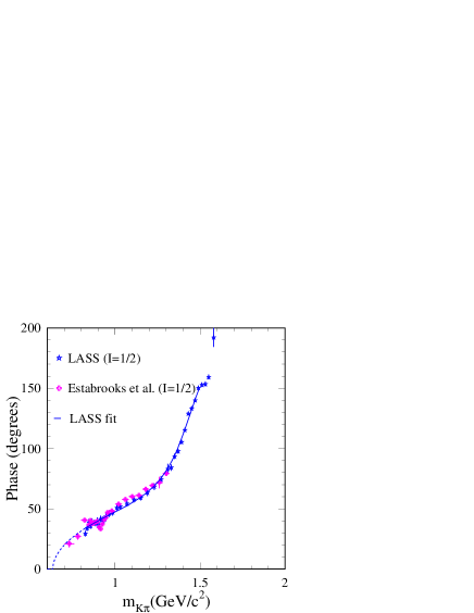
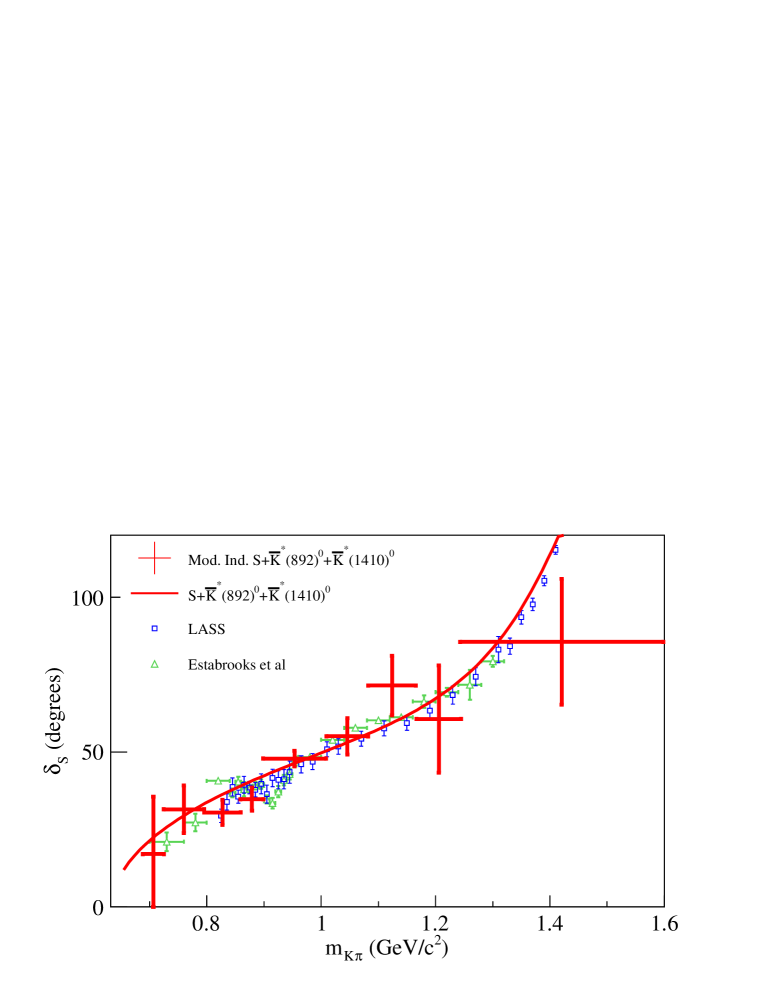
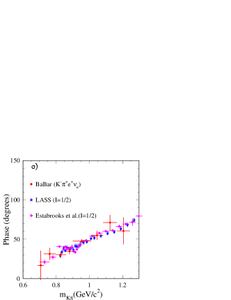
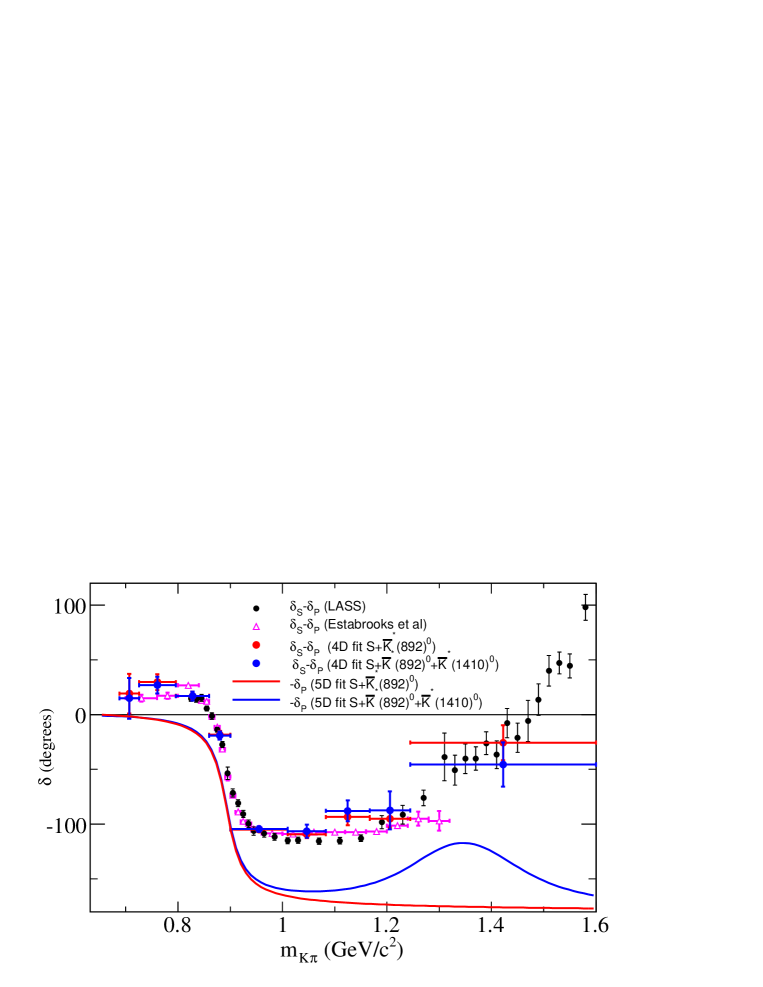
Figure 1: (color online) Comparison between the -wave phase measured in
production at small transfer for several values of
the mass. Results from Ref. ref:easta1 are limited
to to remain in the elastic regime
where there is a single solution for the amplitude.
The curve corresponds to the
fit given in the second column of Table 3.
III.2 decays
The BABAR and Belle collaborations ref:taubabar ; ref:taubelle
measured the
mass distribution
in .
Results from Belle were analyzed in Ref. ref:taupich1
using, in addition to the :
•
a contribution from the to the vector form factor;
•
a scalar contribution, with a mass dependence compatible with LASS
measurements but whose branching fraction was not provided.
Another interpretation of these data was given in Ref. ref:mouss2 .
Using the value of the rate determined from Belle data,
for the , its relative contribution to the
channel was evaluated
to be of the order of .
III.3 Hadronic meson decays
interactions were studied in several Dalitz plot analyses of
three-body decays
and we consider only
as measured by the E791 ref:e791kpipi , FOCUS ref:focuskpipi ; ref:focuskpipi2 ,
and CLEO-c ref:kpipi_cleoc collaborations.
This final state is known to have a large -wave component because
there is no resonant contribution to the
system.
In practice each collaboration has developed various approaches and results
are difficult to compare.
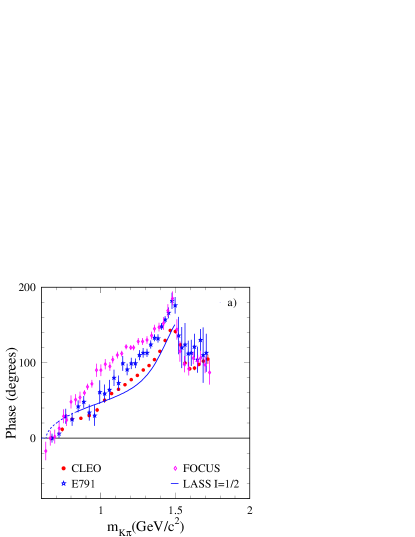
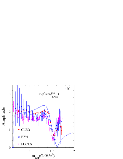
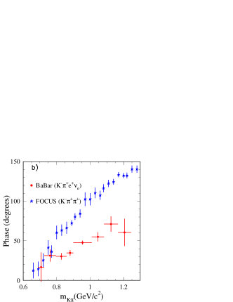
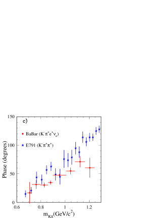
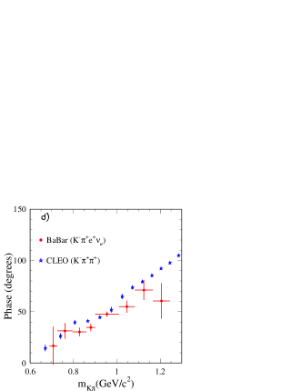
Figure 2: (color online) a) Comparison between the -wave phase measured in
various experiments analyzing the
channel (E791 ref:e791kpipi ,
FOCUS ref:focuskpipi ; ref:focuskpipi2
and CLEO ref:kpipi_cleoc ) and a fit to LASS data (continuous line). The dashed line
corresponds to the extrapolation of the fitted curve. Phase measurements
from decays are shifted to be equal to zero at
. b) The -wave amplitude magnitude measured in
various experiments
is compared with the elastic expression.
Normalization is arbitrary between the various distributions.
The -wave phase measured by these collaborations is
compared in Fig. 2-a with the phase of
the () amplitude determined from LASS data. Measurements
from decays are shifted so that the phase is equal
to zero for .
The magnitude of the amplitude obtained
in Dalitz plot analyses is compared
in Fig. 2-b
with the “naive” estimate
given in Eq. (4), which is derived
from the elastic () amplitude fitted to LASS data.
By comparing results obtained by the three experiments analyzing
, several remarks are formulated.
•
A component is included only in the CLEO-c
measurement and it corresponds to of the decay rate.
•
The relative importance of
and components can be different in scattering and
in a three-body decay. This is because, even if Watson’s theorem
is expected to be valid, it applies separately for the
and components and concerns only the corresponding
phases of these amplitudes.
In E791 and CLEO-c they measured the total
-wave amplitude and compared their results with the
component from LASS. FOCUS ref:focuskpipi , using the phase
of the amplitude
measured in scattering experiments, had fitted separately the two
components and found large effects from the part.
In Fig. 2-a the phase of the total -wave amplitude
which contains contributions from the two isospin components,
as measured by FOCUS ref:focuskpipi2 ,
is plotted.
•
Measured phases in Dalitz plot analyses have a global shift as compared
to the scattering case (in which phases are expected to be zero at
threshold). Having corrected for this effect (with some arbitrariness),
the variation measured for the phase in three-body decays and in
scattering is roughly similar, but quantitative comparison is difficult.
Differences between the two approaches
as a function of
are much larger than the quoted uncertainties.
They may arise from the comparison
itself, which considers the total -wave in one case and only the
component for scattering. They could be due also to the interaction
of the bachelor pion which invalidates the application of the
Watson theorem.
It is thus difficult to draw quantitative conclusions from results
obtained with decays. Qualitatively,
one can say that the
phase of the -wave component depends roughly similarly on
as the phase measured by LASS.
Below the , the
-wave amplitude magnitude has a smooth variation versus .
At the average mass value and above, this magnitude has a sharp
decrease with the mass.
III.4 decays
The dominant hadronic contribution in the
decay channel comes from the
( =) resonant state. E687 ref:e687
gave the first suggestion for an additional component.
FOCUS ref:focus1 , a few years later, measured the -wave contribution
from the asymmetry in the angular distribution of the in
the rest frame. They concluded that the phase
difference between - and -waves was compatible with a constant equal
to , over the mass region.
In the second publication ref:focus2 they
found that the asymmetry could be explained if they used
the variation of the -wave component
versus the mass
measured by the LASS collaboration ref:lass1 .
They did not fit to their data the two parameters that governed
this phase variation but
took LASS results:
(11)
These values corresponded to the total -wave amplitude
measured by LASS which
was the sum of and contributions whereas only the former
component was present in charm semileptonic decays.
For the -wave amplitude they assumed that it was proportional to
the elastic amplitude (see Eq. (4)).
For the -wave, they used a relativistic Breit-Wigner with mass
dependent width
ref:angles .
They fitted the values of the pole mass, the width and the
Blatt-Weisskopf damping
parameter for the .
These values from FOCUS are given in Table 4
and compared with present world averages ref:pdg10 .
, dominated
by the -wave measurements from LASS.
Table 4: Parameters of the measured by FOCUS are compared
with world average or previous values.
They also compared the measured angular asymmetry of the in the rest frame versus the mass with
expectations from a resonance and conclude that the presence of a could
be neglected.
They used a Breit-Wigner distribution for the amplitude using
values measured by the E791 collaboration ref:e791kappa for the mass and width of this resonance
().
This approach to search for a does not seem to be appropriate.
Adding a in this way violates the Watson theorem as the phase
of the fitted amplitude would differ greatly from the one measured by LASS.
In addition, the interpretation of LASS measurements in Ref. ref:seb1
concluded there was evidence for a .
In addition to the they measured the rate
for the non-resonant -wave contribution and placed
limits on other components
(Table 5).
Table 5: Measured fraction of the non-resonant -wave component
and limits on contributions from and
in the decay , obtained by FOCUS
ref:focus2 .
Analyzing events from a sample
corresponding to integrated luminosity, the CLEO-c collaboration
had confirmed the FOCUS result for the -wave contribution. They did
not provide an independent measurement of the -wave phase ref:cleoc1 .
IV decay rate formalism
The invariant matrix element for the
semileptonic decay is the product of a hadronic and a leptonic current.
(12)
In this expression, are
the , and four-momenta, respectively.
The leptonic current corresponds to the
virtual which decays into .
The matrix element of the hadronic current can be written in terms
of four form factors, but
neglecting the electron mass, only three are contributing to the
decay rate: and .
Using the conventions of Ref. ref:wise1 ,
the vector and axial-vector components are, respectively:
(13)
(14)
As there are 4 particles in the final state,
the differential decay rate has five degrees of freedom
that can be expressed in the following variables
ref:cab1 ; ref:pais1 :
•
, the mass squared of the system;
•
, the mass squared of the system;
•
, where is the angle between the
three-momentum in the rest frame and the line of flight
of the in the rest frame;
•
, where is the angle between the
charged lepton three-momentum in the rest frame and the line of flight
of the in the rest frame;
•
, the angle between the normals to the planes defined in the
rest frame by the pair and the pair.
is defined between and .
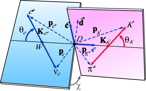
Figure 3: (color online) Definition of angular variables.
The angular variables are shown in Fig. 3,
where is the three-momentum in the CM and is the
three-momentum of the positron in the virtual CM.
Let be the unit vector along the direction in the rest frame,
the unit vector along the projection of perpendicular
to , and the unit vector along the projection of
perpendicular to .
We have:
(15)
The definition of is the same as proposed initially in
Ref. ref:cab1 .
When analyzing decays, the sign of
has to be changed. This is because, if invariance is assumed
with the adopted definitions, changes sign through
transformation of the final state ref:focus1 .
For the differential decay partial width,
we use the formalism given in Ref. ref:wise1 , which generalizes
to five variables
the decay rate given in Ref. ref:rich1 in terms of
and variables.
In addition, it provides a partial wave decomposition for the hadronic system.
Any dependence on the lepton mass is neglected as only electrons
or positrons are used in this analysis:
(16)
In this expression,
where is the momentum
of the system in the rest frame, and .
is the breakup momentum of the system in its rest frame.
The form factors and , introduced in
Eq. (13-14),
are functions of , and
.
In place of these form factors and to simplify the notations,
the quantities are defined ref:wise1 :
(17)
The dependence of on and is given by:
where depend on and .
These quantities can be expressed in terms of the three form factors,
.
(19)
Form factors can be expanded into partial waves
to show their explicit dependence on . If only
-, - and -waves are kept, this gives:
(20)
Form factors depend on and .
characterizes the -wave contribution whereas
and correspond to the - and -wave, respectively.
IV.1 -wave form factors
By comparing expressions given in Ref. ref:wise1 and
ref:rich1 it is possible to relate
with the helicity form factors :
(21)
where is a constant factor, its value is given in Eq. (26);
it depends on the definition adopted for the mass distribution.
The helicity amplitudes can in turn be related to the two
axial-vector form factors , and to the vector form factor
:
(22)
As we are considering resonances which have an extended
mass distribution, form factors
can also have a mass dependence. We have assumed that the
and dependence can be factorized:
(23)
where in case of a resonance is
assumed to behave according to a Breit-Wigner distribution.
This factorized expression can be justified by the fact that the
dependence of the form
factors is expected to be determined by the singularities
which are nearest to the physical region:
. These singularities are poles
or cuts situated at (or above) hadron masses -, depending on the form factor.
Because the variation range is limited
to , the proposed approach is equivalent
to an expansion in .
For the dependence we use a single pole parameterization
and try to determine the effective pole mass.
(24)
where and are expected to be close to
and respectively. Other parameterizations
involving a double pole in have been proposed
ref:doublepole , but as the present
analysis is not sensitive to , the single pole ansatz is adequate.
Ratios of these form factors, evaluated at ,
and , are measured
by studying the variation of the differential
decay rate versus the kinematic variables.
The value of is determined by measuring
the
branching fraction.
For the mass dependence, in case
of the , we use a Breit-Wigner distribution:
(25)
In this expression:
•
is the pole mass;
•
is the total width of the for ;
•
is the mass-dependent width:
;
•
where is
the Blatt-Weisskopf damping factor: , is the barrier factor,
and are evaluated at the mass and
respectively and depend also on the masses of the decay products.
With the definition of the mass distribution given in Eq. (25),
the parameter entering in Eq. (21) is equal to:
(26)
where .
IV.2 -wave form factor
In a similar way as for the -wave, we need to have the
correspondence between the -wave amplitude (Eq. (IV)) and the corresponding invariant form factor.
In an -wave, only the helicity form factor can contribute
and we take:
(27)
The term is proportional to to ensure that the corresponding decay rate
varies as as expected from the angular momentum between the virtual and the -wave
hadronic state.
Because the variation of the form factor is expected to be determined by the
contribution of states, we use the same dependence as for and .
The term corresponds to the mass dependent -wave amplitude.
Considering that previous charm Dalitz plot analyses have measured
an -wave amplitude magnitude which is essentially constant up to the
mass and then drops sharply above this value, we have used the following ansatz:
(28)
respectively for below and above the pole mass value.
In these expressions, is the -wave phase,
and
. The coefficients have no dimension and their values are fitted, but in practice, the fit to data
is sensitive only to the linear term.
We have introduced the constant
which measures the magnitude of the -wave amplitude.
From the observed asymmetry of the distribution
in our data, . This relative sign between and waves
agrees with the FOCUS measurement ref:focus1 .
IV.3 -wave form factors
Expressions for the form factors
for the -wave are ref:Seb_Dwave :
(29)
These expressions are multiplied by a relativistic Breit-Wigner amplitude
which corresponds to the :
(30)
measures the magnitude of the -wave amplitude and
similar conventions as in Eq. (25)
are used for the other variables
apart from the Blatt-Weisskopf term which is equal to:
(31)
and enters into
(32)
The form factors () are parameterized assuming the
single pole model with corresponding axial or vector poles. Values for these
pole masses are assumed to be the same as those considered before for the
- or -wave hadronic form factors. Ratios of -wave hadronic form factors
evaluated at ,
and are supposed
to be equal to one ref:dwave .
V The BABAR detector and dataset
A detailed description of the BABAR detector and of the algorithms used
for charged and neutral particle reconstruction and identification is
provided elsewhere ref:babar ; ref:babardet .
Charged particles are reconstructed by matching hits in
the five-layer double-sided silicon vertex tracker (SVT)
with track elements in the 40 layer drift chamber (DCH), which is
filled with a gas mixture of helium and isobutane.
Slow particles which due to bending in the T magnetic field
do not have enough hits in the DCH, are reconstructed in the SVT only.
Charged hadron identification is performed combining the measurements of
the energy deposition in the SVT and in the DCH with the information from the
Cherenkov detector (DIRC). Photons are detected and measured in the
CsI(Tl) electro-magnetic calorimeter (EMC).
Electrons are identified by the ratio of the track momentum to the
associated energy deposited in the EMC, the transverse profile of the shower,
the energy loss in the DCH, and the Cherenkov angle in the DIRC.
Muons are identified in the instrumented flux return, composed
of resistive plate chambers and limited streamer tubes interleaved with layers of steel and brass.
The results presented here are obtained using
a total integrated luminosity of .
Monte Carlo (MC) simulation samples of decays,
charm, and light quark pairs from continuum, equivalent
to times the data statistics,
respectively, and have been
generated using Geant4ref:geant4 . These samples are used mainly
to evaluate background components. Quark fragmentation in continuum events is described
using the JETSET package ref:jetset .
The MC distributions are rescaled to the
data sample luminosity, using the expected cross sections
of the different components : nb for ,
nb for and , and nb for light , , and quark events.
Dedicated samples of pure
signal events, equivalent to 4.5 times the data statistics,
are used to correct measurements for efficiency and
finite resolution effects.
Radiative decays are modeled by PHOTOS
ref:photos .
Events with a decaying into
are also reconstructed in data and simulation.
This control sample is used to adjust the
-quark fragmentation distribution and the kinematic
characteristics of particles accompanying the
meson in order to better match the data.
It is used also to measure the reconstruction accuracy of the missing
neutrino momentum. Other samples with a , a , or a meson
exclusively reconstructed are used to define corrections on production characteristics
of charm mesons and accompanying particles that contribute to the background.
VI Analysis method
Candidate signal events are isolated from and continuum events
using variables combined into two Fisher discriminants,
tuned to suppress and continuum background events, respectively.
Several differences between distributions
of quantities entering in the analysis, in data and simulation, are
measured and corrected using dedicated event samples.
VI.1 Signal Selection
The approach used to reconstruct mesons decaying into is similar to that
used in previous analyses studying
ref:kenu and ref:kkenu .
Charged and neutral particles are boosted to the CM system and the event thrust axis is determined.
A plane perpendicular to this axis is used to define two hemispheres.
Signal candidates are extracted from a sample of events already enriched in charm semileptonic decays.
Criteria applied for first enriching selection are:
•
an existence of a positron candidate with a momentum larger than in the CM frame,
to eliminate most of light quark events. Positron candidates are
accepted based on a tight identification selection with a pion
misidentified as an electron or a positron below one per
mill;
•
a value of , being the ratio between
second- and zeroth-order Fox-Wolfram moments ref:r2 , to decrease
the contribution from decays;
•
a minimum value
for the invariant mass of the particles in the event hemisphere
opposite to the electron candidate, , to reject
lepton pairs and two-photon events;
•
the invariant mass of the system formed by the positron and the most energetic particle in the candidate hemisphere, ,
to remove events where the lepton is the only particle in its hemisphere.
A candidate is a positron, a charged kaon, and a charged pion present in
the same hemisphere.
A vertex is formed using these three tracks, and the
corresponding probability larger than are kept.
The value of this probability is used in the following with other information
to reject background events.
All other tracks in the hemisphere are defined as “spectators”.
They most probably originate from
the beam interaction point and are emitted during hadronization
of the created and quarks. The
“leading” particle is the spectator particle having the highest momentum.
Information from the spectator system is used to decrease the
contribution from the combinatorial background. As charm hadrons take a large
fraction of the charm quark energy, charm decay products
have, on average, higher energies than spectator particles.
To estimate the neutrino momentum, the
system is constrained to the mass.
In this fit, estimates of the direction and of the neutrino energy are
included from measurements obtained from all tracks registered in the event.
The direction estimate is taken as the direction of the vector opposite
to the momentum sum of all reconstructed particles but the kaon, the pion, and the positron.
The neutrino energy is evaluated by subtracting from the hemisphere
energy the energy of reconstructed particles contained in that hemisphere.
The energy of each hemisphere is evaluated by considering that the
total CM energy is distributed between two objects of mass corresponding
to the measured hemisphere masses ref:hemass .
As a is expected to be present in the analyzed hemisphere and as at least
a meson is produced in the opposite hemisphere, minimum values for hemisphere masses are imposed.
For a hemisphere , with the index of the other hemisphere noted as
, the energy and the mass are defined as:
(33)
The missing energy in a hemisphere is the difference between the hemisphere energy and the sum
of the energy of the particles contained in this hemisphere ().
In a given collision, some of the resulting particles might take a path close
to the beam line,
being therefore undetected. In such cases, as one uses all reconstructed
particles in an event to estimate the meson direction,
this direction is poorly determined.
These events are removed by only accepting those in which
the cosine of the angle between the thrust axis and
the beam line, , is smaller than 0.7.
In cases where there is a loss of a large fraction of the energy contained in the opposite hemisphere,
the reconstruction of the is also damaged. To minimize the impact of these cases, events with a missing energy in the opposite
hemisphere greater than 3 are rejected.
The mass-constrained fit also requires estimates
of the uncertainties on the angles defining the direction
and on the missing energy must also be provided. These estimates are parameterized versus the
missing energy in the opposite hemisphere which is used to quantify the quality of the reconstruction in a given event.
Parameterizations of these uncertainties are obtained in data and in simulation using events with a reconstructed
,
for which we can compare the measured direction with its estimate using the algorithm employed
for the analyzed semileptonic decay channel.
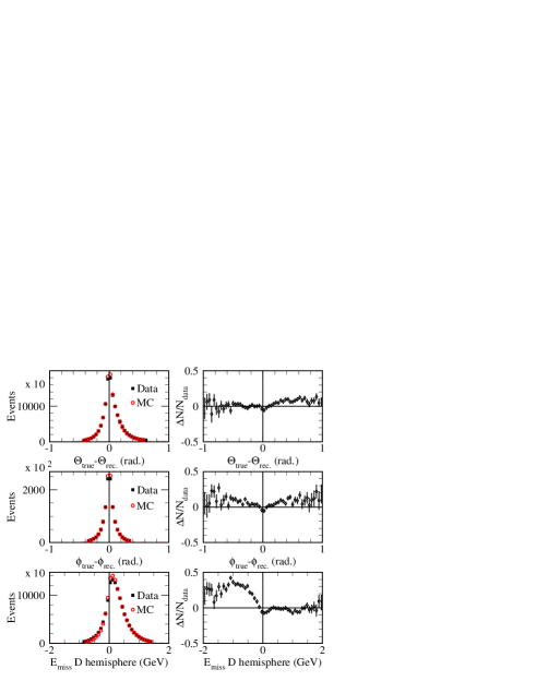
events also allow one to control the missing energy estimate and
its uncertainty. Corresponding distributions obtained in data and with simulated events are given in
Fig. 4. These distributions are similar, and the
remaining differences are corrected as explained in
Section VI.3.2.
Typical values for the reconstruction accuracy of kinematic variables, obtained by
fitting the sum of two Gaussian distributions for each variable, are given in
Table 6. These values are only indicative as the
matching of reconstructed-to-generated kinematic variables of events in five dimensions is included,
event-by-event, in the fitting procedure.
Table 6: Expected resolutions for the five variables. They are obtained
by fitting the distributions to the sum of two
Gaussian functions. The fraction
of events fitted in the broad component is given in the last column.
variable
fraction of events
in broadest Gaussian
0.068
0.325
0.139
0.145
0.5
0.135
0.223
1.174
0.135
0.081
0.264
0.205
0.0027
0.010
0.032
Figure 4: (color online) Distributions of the difference (left)
between reconstructed and expected values, in the CM frame,
for direction angles
() and
for the missing energy in the candidate hemisphere. These distributions
are normalized to the same number of entries.
The is reconstructed in the decay channel.
Distributions on the right display the relative difference between the
histograms given on the left.
VI.2 Background rejection
Background events arise from decays and hadronic
events from the continuum.
Three variables are used to decrease the contribution from events:
, the total charged and neutral
multiplicity, and the sphericity of the system of particles produced in the
event hemisphere opposite to the candidate.
These variables use topological differences between events with decays and
events with fragmentation. The particle distribution in decay events
tends to be isotropic as the mesons are heavy and produced near
threshold, while the distribution in events
is jet-like as the CM energy is well above the charm threshold.
These variables are combined linearly in a Fisher discriminant
ref:fisher , , and corresponding distributions
are given in Fig. 5.
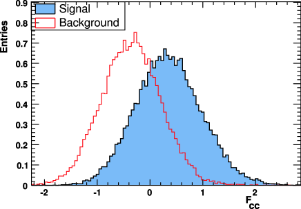
The requirement retains of signal and 15 of -background events.
Figure 5: (color online) Distributions of for signal and for
background events. The two distributions are normalized to the same number of entries.
Background events from the continuum arise mainly from charm particles,
as requiring an electron and a kaon reduces the
contribution from light-quark flavors
to a low level.
Because charm hadrons take a large
fraction of the charm quark energy, charm decay products
have higher average energies and different angular distributions (relative to
the thrust axis or to the direction) as compared to
other particles in the hemisphere, emitted from the hadronization
of the and quarks.
The meson decays also at a measurable distance from the beam interaction
point, whereas background event candidates contain usually a pion
from fragmentation.
Therefore, to decrease the amount of background from fragmentation
particles in events, the following variables are used:
•
the spectator system mass;
•
the momentum of the leading spectator track;
•
a quantity
derived from the probability of the
mass-constrained fit;
•
a quantity
derived from the vertex fit probability of the ,
and trajectories;
•
the value of the momentum
after the
mass-constrained fit;
•
the significance of the flight length of the from the beam interaction point until its decay point;
•
the ratio between the significances of the distance of the pion trajectory
to the decay position and to the beam interaction point.
Several of these variables are transformed such that distributions of
resulting (derived)
quantities have a bell-like shape.
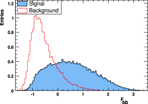
These seven variables are combined linearly into a Fisher discriminant
variable () and the corresponding distribution is given in Fig. 6;
events are kept for values above 0.5.
This selection retains of signal events that were kept by the previous selection requirement
on and
rejects of the remaining background.
About signal events are selected with a ratio . In the
mass region of the this ratio increases to 4.6.
The average efficiency for signal is and is uniform when
projected onto individual kinematic variables.
A loss of efficiency, induced mainly
by the requirement of a minimal energy for the positron, is observed
for negative values of and at low .
Figure 6: (color online) Fisher discriminant variable distribution for charm background and signal events. The two distributions are normalized to the same number of entries.
VI.3 Simulation tuning
Several event samples are used to correct differences between data
and simulation. For the remaining decays, the simulation
is compared to data as explained in Section VI.3.1.
For events,
corrections to the signal sample are different from those to the background
sample. For signal,
events with a reconstructed in data
and MC are used.
These samples allow us to compare the different distributions of the quantities
entering in the definition of the and discriminant
variables. Measured differences are then corrected, as explained below (Section VI.3.2). These samples
are used also to measure the reconstruction accuracy on the direction
and missing energy estimates for .
For background events (Section VI.3.3), the control of the simulation has to be extended
to , and production and to their accompanying
charged mesons.
Additional samples with a reconstructed exclusive decay
of the corresponding charm mesons are used. Corrections are applied also
on the semileptonic decay models such that they agree with recent
measurements. Effects of these corrections are verified using wrong
sign events (Section VI.3.4), which are used also to correct
for the production fractions
of charged and neutral -mesons. Finally, absolute mass
measurement capabilities of the detector and the mass resolution
are verified (Section VI.3.5) using
and
decay channels.
VI.3.1 Background from decays
The distribution of a given variable for events
from the remaining
background is obtained by
comparing corresponding distributions for events registered at the resonance
and 40 below. Compared with expectations from simulated events
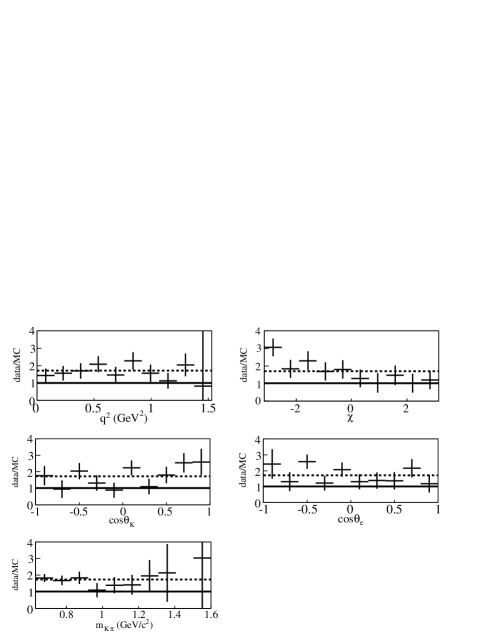
in Fig. 7, distributions versus
the kinematic variables agree reasonably well in shape, within statistics, but the simulation needs to be scaled
by . A similar effect was measured also in a previous
analysis of the decay channel
ref:kkenu .
VI.3.2 Simulation tuning of signal events
Events with a reconstructed candidate
are used to correct the simulation
of several quantities which contribute to the
event reconstruction.
Figure 7: Ratio (data/MC) distribution for decays
versus each of the five kinematic variables. The dotted line corresponds
to data/MC = 1.7.
Using the mass distribution, a signal region,
between 1.849 and 1.889 , and two sidebands
(), are defined.
A distribution of a given variable is obtained by subtracting
from the corresponding distribution of events
in the signal region half the content
of those from sidebands. This approach is
referred to as sideband
subtraction in the following.
It is verified with simulated events that
distributions obtained in this way agree
with those expected from true signal events.
control of the production mechanism:
the Fisher discriminants and are functions
of several variables, listed in Section VI.2,
which have distributions that may differ between data and simulation.
For a given variable, weights are computed
from the ratio
of normalized distributions measured in data and simulation.
This procedure is repeated,
iteratively, considering the various
variables, until
corresponding projected distributions
are similar to those obtained in data.
There are remaining differences between data and simulation coming
from correlations between variables. To minimize their contribution,
the energy spectrum of is weighted
in data and simulation to be similar to the spectrum
of semileptonic signal events.
We have performed another determination of the
corrections without requiring that these
two energy spectra are similar.
Differences between the fitted parameters
obtained using the two sets of corrections are taken as systematic
uncertainties.
control of the direction and missing energy measurements:
the direction of a fully reconstructed
decay is accurately measured and one can therefore compare
the values of the two angles, defining its direction, with those obtained
when using all particles present in the event except those attributed to the
decay signal candidate. The latter procedure is used to estimate
of the direction for
the decay .
Distributions of the difference between angles measured with the
two methods give the corresponding angular resolutions.
This event sample allows also one to compare the missing energy measured in
the hemisphere and in the opposite hemisphere for data and
simulated events. These estimates for the direction and momentum,
and their corresponding
uncertainties are used in a mass-constrained fit.
For this study, differences between data and simulation in
the fragmentation
characteristics are corrected as explained in the previous paragraph.
Global cuts similar to those applied for the
analysis are used such that
the topology of selected events is as
close as possible to that of semileptonic events.
Comparisons between angular resolutions measured in data and simulation
indicate that the ratio data/MC is 1.1
in the tails of the distributions
(Fig. 4).
Corresponding distributions for the missing energy
measured in the signal hemisphere (),
in data and simulation, show that these distributions have an
offset of about 100 (Fig. 4)
which corresponds to energy escaping detection
even in absence of neutrinos. To evaluate the neutrino energy
in semileptonic decays this bias is corrected on average.
The difference between the exact and estimated values of the two angles and
missing energy is measured versus the value of the missing
energy in the opposite event hemisphere ().
This last quantity provides an estimate of the quality of the
energy reconstruction for a given event.
In each
slice of , a Gaussian distribution is fitted and
corresponding values of the average and standard deviation are measured.
As expected, the resolution gets worse when
increases.
These values are used as estimates for the bias and resolution
for the considered
variable.
Fitted uncertainties are slightly higher in data than in the
simulation. From these measurements, a correction and a smearing are defined
as a function of . They are
applied to simulated event estimates of and .
This additional smearing is very small for the direction
determination and is typically on the missing energy estimate.
After applying corrections, the resolution on simulated events becomes slightly
worse than in data.
When evaluating systematic uncertainties we have used the total deviation of
fitted parameters obtained when applying or not applying the corrections.
VI.3.3 Simulation tuning of charm background events from continuum
As the main source of background originates from track combinations in which
particles are from a charm meson decay, and others from hadronization, it is necessary to verify
that the fragmentation of a charm quark into a charm meson and that
the production characteristics of charged particles
accompanying the charm meson are similar
in data and in simulation.
In addition, most background events contain a lepton from a charm hadron semileptonic decay. The simulation
of these decays is done using the ISGW2 model ref:isgw2 ,
which does not agree with recent measurements ref:kenu ,
therefore all simulated decay
distributions are corrected.
Corrections on charm quark hadronization:
for this purpose,
distributions obtained in data and MC are compared. We study the event shape
variables that enter in
the Fisher discriminant and for variables entering into ,
apart from probability of the mass-constrained fit
which is
peculiar to the analyzed semileptonic decay channel.
Production characteristics of charged pions and kaons
emitted during the charm quark fragmentation, are also measured,
and their rate, momentum,
and angle distribution relative to the simulated direction
are corrected. These corrections
are obtained separately for particles having the same or the opposite charge relative to the charm
quark forming the hadron. Corrections consist of a weight
applied to each simulated event. This weight is obtained iteratively,
correcting in turn each of the considered distributions.
Measurements are done for , (vetoing from decays) and for .
For mesons, only the corresponding -quark fragmentation distribution
is corrected.
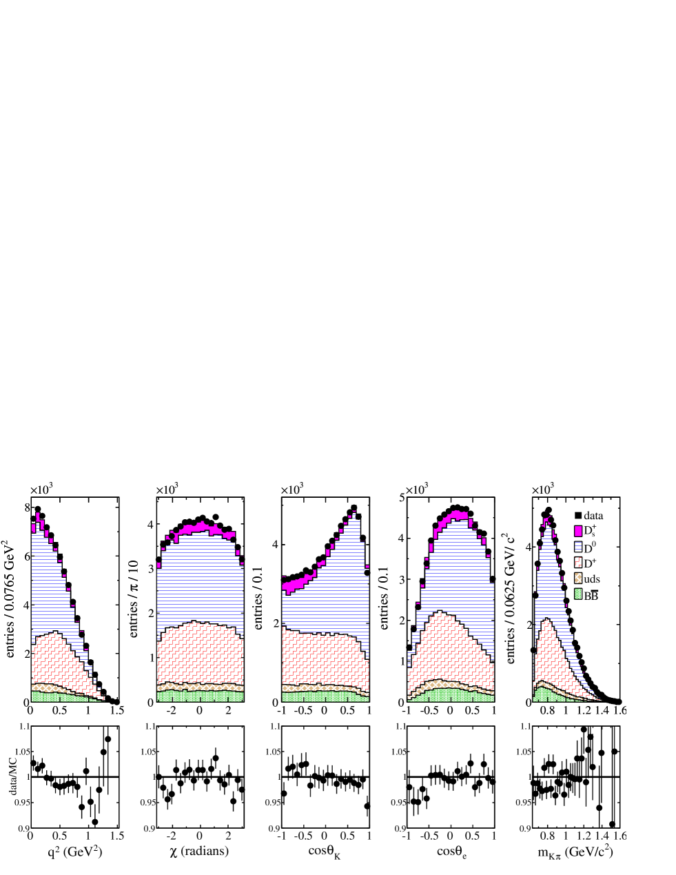
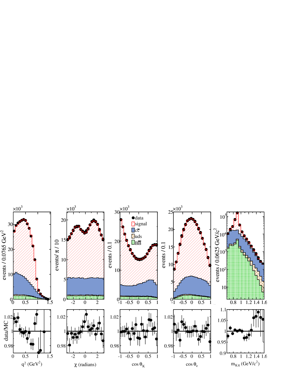
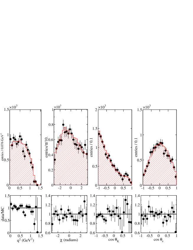
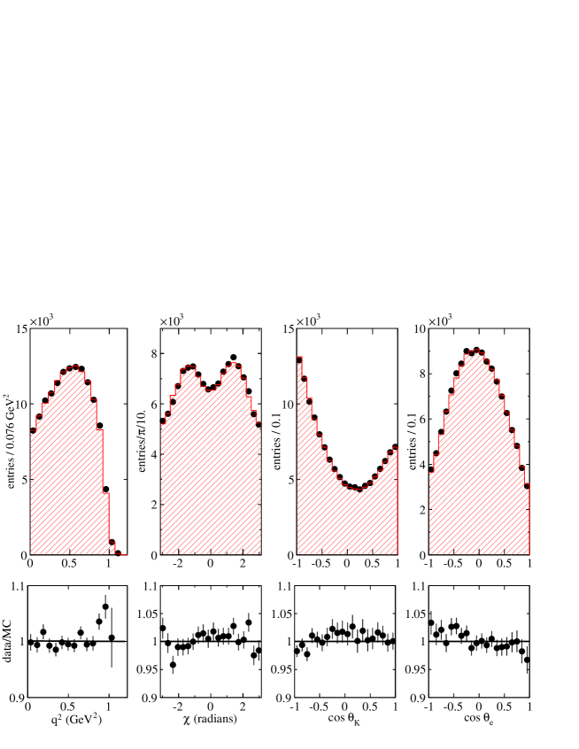
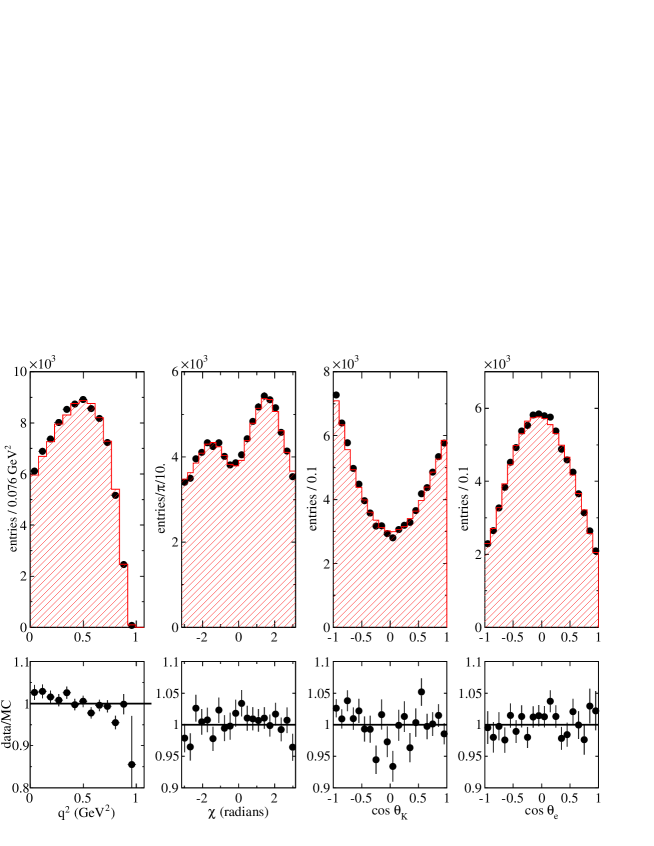
Figure 8: (color online) Distributions of the five dynamical variables for
wrong-sign events in data (black dots) and MC (histograms),
after all corrections. From top to bottom the background components displayed in the stacked
histograms are: events respectively.
In the lower row, distributions of the ratio data/MC for upper row plots are given.
Correction of D semileptonic decay form factors:
by default, semileptonic decays are generated in EvtGen ref:evtgen using the ISGW2 decay model
which does not reproduce present measurements (this was shown for instance in the BABAR analysis
of ref:kenu ).
Events are weighted such that
they correspond to hadronic form factors behaving according to the
single pole parameterization as in Eq. (24).
For decay processes of the type ,
where is a pseudoscalar meson,
the weight is
proportional to the square of the ratio between
the corresponding hadronic form factors, and
the total decay branching fraction
remains unchanged after the transformation.
For all Cabibbo-favored decays a pole mass value equal to
ref:kenu is used
whereas for Cabibbo-suppressed decays ref:cleo_pienu
is taken. This value of the pole mass is used
also for semileptonic decays into a pseudoscalar meson.
For decay processes of the type , where and are respectively pseudoscalar and vector mesons,
corrections depend on the mass of the hadronic system, and on and .
They are evaluated iteratively using projections of the differential
decay rate versus these variables, as obtained in EvtGen and in a
simulation which contains the expected distribution.
To account for correlations between these variables,
once distributions agree in projection, binned distributions over the
five dimensional space are compared and a weight is measured in each bin.
For Cabibbo-allowed decays, events are distributed over 2800 bins,
similar to those defined in Section VI.4; 243 bins
are used for Cabibbo-suppressed decays.
Apart for the resonance mass and width which are different
for each decay channel, the same values, given in Table
7, are used for the other parameters
which determine the differential decay rate.
For decay channels an -wave component
is added with the same characteristics as in the present measurements.
Other decay channels included in EvtGen ref:evtgen
and contributing to this same final
state,
such as a constant amplitude and
the components, are removed as they are
not observed in data.
All branching fractions used in the simulation agree within uncertainties
with the current measurements ref:pdg10
(apart for , which is then rescaled).
Only the shapes of charm semileptonic decay distributions are corrected.
Systematic uncertainties related to these corrections are estimated
by varying separately each parameter according to its expected uncertainty,
given in Table 7.
Table 7: Central values and variation range for the various
parameters which determine the differential decay rate
in decays, used to correct the simulation
and to evaluate corresponding systematic uncertainties. The
form factors
and the mass parameters and are defined in
Eq. (24).
parameter
central
variation
value
interval
VI.3.4 Wrong sign event analysis
Wrong-sign (WS) events of the type are used
to verify if corrections applied to the simulation improve the
agreement with data,
because the origin of these events is quite similar to that of the background
contributing in right-sign (RS) events.
The ratio between the measured and expected number of WS events is . In RS events the
number of background candidates is a free parameter in the fit.
At this point corrections have been evaluated separately for charged and
neutral mesons. As the two charged states correspond to background
distributions having different shapes, it is also possible to correct for
their relative contributions. We improve the agreement with data by increasing
the fraction of events with a meson in MC by 4
and correspondingly decreasing the fraction of by .
After corrections, projected distributions of the five kinematic variables obtained in data and simulation
are given in Fig. 8.
VI.3.5 Absolute mass scale.
The absolute mass measurement is verified using exclusive
reconstruction of charm mesons in data and simulation.
For candidate events
,
the mean and RMS values of the
mass distribution are measured from a fit of
the sum to a Gaussian distribution for the signal and a first
order polynomial for the background.
The mass reconstructed in simulation is very close
to expectation, , whereas
in data it differs by .
Here is the difference between the reconstructed and the
exact or the world average mass values when analyzing MC or data respectively.
The uncertainty quoted for is from Ref. ref:pdg10 .
To correct for this effect the momentum () of each track in data, measured
in the laboratory frame, is increased by an amount:
. The standard deviation
of the Gaussian fitted on the signal is slightly
smaller in simulation, , than in data,
. The difference
between the widths of reconstructed signals in the two samples,
is measured versus the
transverse momentum of the tracks emitted in the decay.
In simulation, the measured transverse momenta of the
tracks
are smeared to correct for this difference.
Having applied these corrections, mass distributions,
for the decay obtained in data and
simulation are compared. The standard deviation of the fitted
Gaussian distribution on signal is now similar in data and simulation.
The reconstructed mass is higher by in simulation
(on which no correction was applied) and by in data.
These remaining differences are not corrected and included as
uncertainties.
VI.4 Fitting procedure
A binned distribution of data events is analyzed.
The expected number of events in each bin depends on signal and background estimates and
the former is a function of the values of the fitted parameters.
We perform a minimization of a negative log-likelihood
distribution. This distribution has two parts. One corresponds
to the comparison between measured and expected number of events in
bins which span the five dimensional
space of the differential decay rate. The other part uses the distribution of the values
of the Fisher discriminant variable to measure the fraction of background events.
There are respectively 5, 5 and 4 equal size bins for the variables ,
and . For and we use respectively 4 and 7 bins of different size
such that they contain approximately the same number of signal events.
There are 2800 bins () in total.
The likelihood expression is:
(34)
where is the number of data events in bin
and is the sum of MC estimates for
signal and background events in the same bin.
is the Poisson probability
for having
events in bin where
events are expected,
on average, where:
(35)
The summation to determine extends over all generated
signal events which are reconstructed in bin .
The terms are, respectively, the values of parameters used in the fit and
those used to produce simulated events. is the value of
the expression for the decay rate (see Eq. (16)) for event
using the set of parameters .
In these expressions, generated values of the kinematic variables are used.
is the weight applied to each signal event to correct for
differences between data and simulation. It is left unchanged during the fit.
is the estimated number of background events in bin
given by the simulation, corrected for measured differences
with data, as explained in Section VI.3.
is the estimated total number of background events.
and are respectively the total number of signal and
background events fitted in the data sample which contains events.
and are the probability density functions for signal and background, respectively,
evaluated at the value of the variable for event .
The following expressions are used :
(36)
and values of the corresponding parameters
and
are determined from fits to binned distributions of
in simulated signal and background samples.
and are normalization
factors.
In Fig. 9 these two distributions are drawn to illustrate
their different behavior versus the values of for signal and
background events. As expected, the
distribution has higher
values at low than the corresponding distribution for signal.
VI.4.1 Background smoothing
As the statistics of simulated background events for the charm continuum is only times the data,
biases appear in the determination of the fit parameters if we use simply, as estimates for background in each bin,
the actual values obtained from the MC.
Using a parameterized event generator, this effect is measured using
distributions of the difference between the fitted and exact values of a
parameter divided by its fitted uncertainty (pull distributions).
To reduce these biases, a smoothing ref:Cranmer of
the background distribution is performed.
It consists of distributing the contribution of
each event, in each dimension, according to a Gaussian distribution.
In this procedure correlations between variables are neglected.
To account for boundary effects, the dataset is reflected about each boundary.
is essentially uncorrelated with all other variables and
in particular with . Therefore,
for each bin in (), a smoothing
of the and distributions is done in the hypothesis
that these two variables are independent.
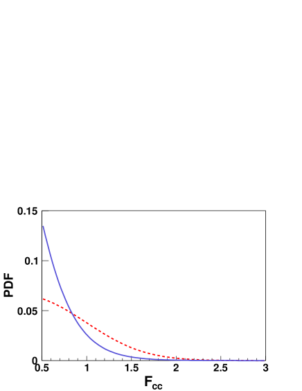
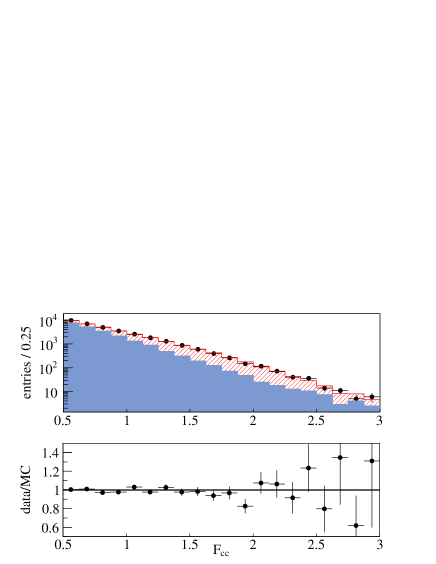
Figure 9: (color online) Probability density functions for signal (red dashed line) and
background (blue full line) events versus the values of the discriminant variable .
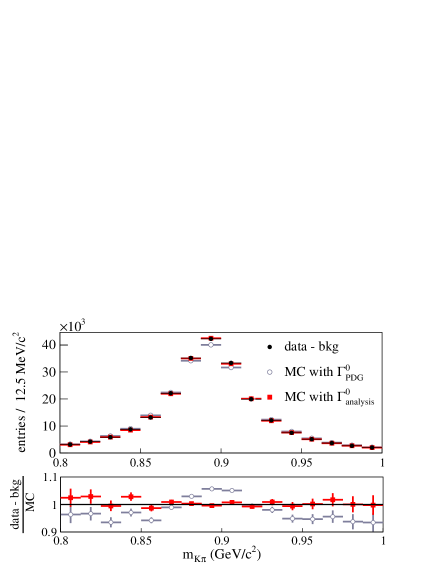
VII hadronic form factor measurements
We first consider a signal made of the and -wave components.
Using the LASS parameterization of the -wave phase versus the mass (Eq. (10)),
values of the following quantities
(quoted in Table 8 second column) are obtained from a fit to data :
•
parameters of the Breit-Wigner distribution: , , and , the Blatt-Weisskopf
parameter;
•
parameters of the hadronic form factors: , and . The parameter
which determines the variation of the vector form factor is fixed to ;
•
parameters which define the -wave component: and for the amplitude
(Eq. (28)), and for the phase (Eq. (8));
•
and finally the total numbers of signal and background events,
and .
Table 8: Values of fitted parameters assuming that the final state consists of a
sum of -wave and components (second column), includes the
in the -wave (third column) and a -wave (last column).
The variation of the -wave phase versus the mass is parameterized according to
Eq. (10) whereas the -wave amplitude is parameterized as in Eq. (28).
Fit results including the are discussed in Section VIII.1.
Values given in the third column of this Table are the central results
of this analysis.
variable
fixed
fixed
fixed
fixed
Fit probability
Apart from the effective range parameter, , all other quantities are accurately measured.
Values for the -wave parameters depend on the parameterization used for the -wave and as the LASS
experiment includes a and other components one cannot directly compare our results on and
with those of LASS.
We have obtained the first measurement for which gives the
variation of the axial vector hadronic form factors.
Using the values of fitted parameters and integrating
the corresponding differential decay rates, fractions of - and -wave
are given in the second column of Table 9.
Table 9: Fractions for signal components assuming that the final state consists of a
sum of -wave and components (second column), including the
in the -wave (third column) and a -wave (last column).
In the second and third cases, the sum of the fractions for the two
does not correspond exactly
to the total -wave fraction because of interference.
Component
-wave
-wave
-wave
Projected distributions, versus the five variables, obtained in data and from the -wave + fit result are displayed
in Fig. 10.
The total of this fit is 2914 for 2787 degrees of freedom which corresponds to the probability of 4.6.
Fit results including the and -wave are discussed
in Section VIII.
Figure 10: (color online) Projections of data (black dots) and of the fitted MC
distribution (histograms)
versus each of the five kinematic variables.
The signal contains an -wave and a components.
From top to bottom the fitted background components displayed
in the stacked
histograms are: events respectively.
In the lower row, distributions of the ratio data/MC for upper row plots
are given.
VII.1 Systematic uncertainties
The systematic uncertainty on each fitted parameter () is defined
as the difference between the fit results in nominal conditions
and those obtained, , after changing a variable or a condition ()
by an amount which corresponds to an estimate of the uncertainty
in the determination of this quantity:
(37)
Values are given in Table 10.
Some of the corrections induce a variation on the
distributions for signal or background which are therefore
reevaluated.
VII.1.1 Signal production and decay
Corrections of distributions of Fisher input variables (I):
the signal control sample is corrected as explained in
Section VI.3.2.
The corresponding systematic uncertainty
is obtained by defining new event weights without taking into account
that the momentum distribution of reconstructed mesons is different in hadronic
and in semileptonic samples.
Simulation of radiative events (II):
most of radiative events correspond to radiation from the charged lepton, although a non-negligible fraction comes
from radiation of the decay products.
In , by comparing two generators (PHOTOS
ref:photos and KLOR ref:klor ), the CLEO-c collaboration has used a variation of
to evaluate corresponding systematic uncertainties ref:cleocrad .
We have increased the fraction of radiative events (simulated by PHOTOS) by 30 (keeping constant the total number of events) and obtained
the corresponding variations on fitted parameters.
Table 10: Systematic uncertainties on parameters fitted using
the -wave and model, expressed as : (I) uncertainty associated with the tuning of the signal control sample,
(II) fraction of radiative signal events increased by , (III) no PID
corrections on electron or kaon in MC signal events,
(IV) no smearing applied on for simulated signal events, (V) background rate lowered by
the statistical uncertainty
of its determination, (VI) uncertainty associated with the tuning of fragmentation in charm background events, (VII) remaining uncertainty on semileptonic
decay models in charm background events, (VIII) uncertainty associated with c-meson relative fractions,
(IX) uncertainty remaining from the smoothing of the background distribution, (X) effects from limited statistics in simulation, (XI) variation of parameters
that were kept constant in the fit and, (XII) absolute mass scale uncertainties.
variation
signal
I
-0.13
-0.16
-0.10
-0.18
0.28
0.18
-0.40
-0.43
0.02
0.00
-0.36
0.44
II
-0.36
0.07
0.02
-0.11
0.34
0.10
0.26
0.20
0.17
0.21
-0.21
0.26
III
0.21
0.13
0.27
0.69
0.78
0.51
0.17
0.16
0.29
0.17
0.18
0.22
IV
0.29
0.36
0.20
-0.18
0.07
-0.25
0.15
0.19
-0.31
-0.23
0.57
-0.70
bkg.
V
-0.06
0.32
0.09
0.22
-0.13
0.03
0.30
0.31
0.14
0.30
-0.09
0.11
bkg.
VI
-0.04
0.21
-0.61
0.10
-0.08
0.07
0.33
0.32
0.13
0.27
0.06
-0.08
VII
0.53
0.19
0.14
0.16
0.13
0.07
0.10
0.10
0.17
0.19
0.16
0.22
VIII
0.24
0.36
0.11
-0.49
0.85
0.04
-0.76
-0.68
-0.77
1.02
0.76
-0.91
Fitting procedure
IX
0.13
0.17
0.25
0.29
0.30
0.25
0.25
0.25
0.32
0.32
0.13
0.13
X
0.70
0.70
0.70
0.70
0.70
0.70
0.70
0.70
0.70
0.70
0.70
0.70
XI
0.00
0.00
0.07
0.07
1.15
0.08
0.05
0.05
1.43
0.46
0.01
0.01
XII
-0.93
-0.06
0.09
0.09
-0.05
0.04
0.03
0.02
0.07
-0.05
0.00
0.00
1.41
1.00
1.06
1.21
1.87
0.97
1.27
1.23
1.87
1.47
1.29
1.48
Particle identification efficiencies (III):
the systematic uncertainty is estimated by not correcting for
remaining differences between data and MC on particle identification.
Estimates of the values and uncertainties for the direction and missing energy (IV):
in Section VI.3.2 it is observed that estimates of the
direction and energy are more accurate in the simulation than in data.
After applying smearing corrections, the result of this comparison is reversed.
The corresponding systematic uncertainty is equal to the difference on fitted
parameters obtained with and without smearing.
VII.1.2 background correction (V)
The number of remaining background events
expected from simulation is rescaled by
(see Section VI.3.1).
The uncertainty on this quantity is used to evaluate corresponding systematic uncertainties.
after applying corrections explained in Section VI.3.3, the
remaining differences between data and simulation for the considered distributions are five times smaller.
Therefore, 20 of the
full difference measured before applying corrections
is used as the systematic uncertainty.
Form-factor correction systematics (VII):
corresponding systematic uncertainties depend on uncertainties
on parameters used to model the differential semileptonic decay
rate of the various charm mesons (see Section VI.3.3).
using WS events, it is found in Section VI.3.4
that the agreement between data and simulation
improves by changing the hadronization fraction of the different charm mesons.
Corresponding variations of relative hadronization fractions are
compatible with current experimental uncertainties on these quantities.
The corresponding systematic uncertainty is obtained by not applying
these corrections.
VII.1.4 Fitting procedure
Background Smoothing (IX):
the MC background distribution is smoothed as explained in Section VI.4.1.
The evaluation of the associated systematic uncertainty is performed
by measuring with simulations based on parameterized distributions,
the dispersion of displacements of the fitted quantities
when the smoothing is or is not applied in a given experiment.
It is verified that uncertainties on the values of the two parameters
used in the smoothing have negligible contributions to the resulting
uncertainty.
Limited statistics of simulated events (X):
fluctuations of the number of MC events in each bin are
not included in the likelihood expression, therefore one quantifies this
effect using fits on distributions obtained with a parameterized event
generator.
Pull distributions of fitted parameters, obtained in similar conditions as in data, have an RMS of 1.2.
This increase is attributed to the limited MC statistics used for the signal (4.5 times the data)
and, also, from the available statistics used to evaluate the
background from continuum events.
We have included this effect as a systematic uncertainty corresponding to 0.7 times the quoted
statistical uncertainty of the fit. It corresponds to the additional
fluctuation needed to obtain a standard deviation of 1.2 of the pull
distributions.
VII.1.5 Parameters kept constant in the fit (XI).
The signal model has three fixed parameters, the vector pole mass
and the mass and width of the resonance.
Corresponding systematic uncertainties are obtained by varying the values of these parameters.
For a variation is used, whereas for the other two quantities we take
respectively and ref:pdg10 .
VII.1.6 Absolute mass scale (XII).
When corrections defined in Section VI.3.5 are applied,
in data and simulation, for
the decay channel, the fitted
mass in data increases by and its
width decreases by .
The uncertainty on the absolute mass measurement of the
is obtained by noting that a mass variation, ,
of the reference signal
is reduced by a factor of four in the mass region; this gives:
(38)
In this expression, is the uncertainty on the
mass ref:pdg10 and is the difference between
the reconstructed
and exact values of the mass in
Table 11: Systematic uncertainties on parameters fitted using
a model for the signal which contains -wave, and components, expressed as : (I) uncertainty associated with the tuning of the signal control sample,
(II) fraction of radiative signal events increased by ,
(III) no PID corrections on electron or kaon in MC signal events,
(IV) no smearing applied on for simulated signal events, (V) background rate lowered by
the statistical uncertainty
of its determination, (VI) uncertainty associated with the tuning of
fragmentation in charm background events, (VII) remaining uncertainty
on semileptonic
decay models for background events, (VIII) uncertainty associated with c-meson relative fractions,
(IX) uncertainty remaining from the smoothing of the background distribution, (X) effects from limited statistics in simulation, (XI) variation of parameters
that were kept constant in the fit, (XII) uncertainties on absolute mass scale.
variation
signal
(I)
0.17
0.05
-0.23
-0.22
-0.31
0.18
0.14
-0.14
-0.13
0.23
-0.19
-0.39
0.45
(II)
-0.18
0.06
-0.01
-0.14
-0.36
0.09
-0.10
0.08
0.05
-0.08
-0.08
-0.23
0.26
(III)
0.02
0.10
0.06
0.70
0.73
0.53
0.14
0.07
0.41
0.08
0.22
0.10
0.12
(IV)
-0.13
0.03
0.29
-0.18
-0.04
-0.27
-0.02
0.02
-0.17
-0.18
0.32
0.61
-0.70
bkg.
(V)
-0.41
-0.04
0.34
0.26
0.16
0.05
-0.12
0.12
0.08
-0.46
0.22
-0.01
0.02
bkg.
(VI)
-0.14
0.07
-0.08
0.13
0.09
0.09
-0.16
0.14
-0.01
-0.24
-0.03
0.08
-0.09
(VII)
0.09
0.08
0.14
0.19
0.14
0.08
0.18
0.15
0.06
0.10
0.11
0.14
0.18
(VIII)
-0.44
-0.19
0.59
-0.48
-0.75
0.04
0.98
-0.94
0.28
-0.42
-0.21
1.03
-1.23
Fitting procedure
(IX)
0.13
0.17
0.25
0.29
0.30
0.25
0.25
0.25
0.32
0.30
0.30
0.13
0.13
(X)
0.70
0.70
0.70
0.70
0.70
0.70
0.70
0.70
0.70
0.70
0.70
0.70
0.70
(XI)
0.27
0.12
0.29
0.07
1.15
0.08
0.57
0.55
3.25
0.89
0.40
0.09
0.10
(XII)
-0.33
-0.05
0.03
0.09
0.05
0.04
-0.05
0.03
0.06
-0.02
-0.01
-0.02
0.02
1.08
0.78
1.13
1.24
1.81
0.99
1.40
1.35
3.39
1.39
1.02
1.48
1.69
simulation (see Section
VI.3.5).
Uncertainty on the width measurement from track resolution effects
is negligible.
VII.1.7 Comments on systematic uncertainties
The total systematic uncertainty is obtained by summing in quadrature
the various contributions.
The main systematic uncertainty on comes from the assumed
variation for the parameter because these two parameters
are correlated. Values of the parameters and
depend on the mass
and width of the because the measured -wave phase
is the sum of two components: a background term and the .
Figure 11: (color online) Projections of data (black dots) and of the fitted
MC distribution (histograms)
versus each of the five kinematic variables.
The signal contains -wave, and components.
From top to bottom the background components displayed in the stacked
histograms are: events respectively.
In the lower row, distributions of the ratio data/MC for upper row plots
are given.
VIII Including other components
A contribution to the -wave from the radial excitation
was measured by LASS ref:lass1 in interactions
at small transfer and in decays ref:taubelle .
As is discussed in the following, even if the statistical significance
of a signal at high mass does not reach the level to claim an observation,
data favor such a contribution and a signal containing the
, the and an -wave components is considered as our
nominal fit to data.
To compare present results for the -wave with LASS measurements
a possible contribution from the is included in the signal model.
It is parameterized using a similar Breit-Wigner expression as for the
resonance.
The L=1 form factor components are in this case written as:
(39)
where stands for the Breit-Wigner distribution (Eq. (25)) and for that of the .
As the phase space region where this last component contributes is scarcely populated (high mass),
this analysis is not highly sensitive to the exact shape of the resonance.
Therefore the Breit-Wigner parameters of the
(given in Table 1) are fixed and
only the relative strength () and phase () are fitted.
For the same reason, the value of
is fixed to the LASS result (given in Table 3).
Figure 12: (color online) Comparison between measured and fitted distributions
of the values of the discriminant variable. Points with
error bars correspond to data. The histogram is the fitted distribution.
It is the sum of a background (blue, filled histogram) and signal (hatched)
components.
Figure 13: (color online) Comparison between measured and fitted mass distributions
in the region. Results of a fit in which the width of the
meson is fixed to (value quoted in 2008 by the Particle Data Group) are also given.
VIII.1 Results with a contribution included
Results are presented in Table 8 (third column)
using the same -wave parameterization
as in Section VII. They correspond to the central results
of this analysis.
Figure 14: (color online) Background subtracted data mass distribution (black full dots)
and fit result (red open crosses) for the -wave and model (left)
and the -wave, and model (right), in the high mass region.
Error bars correspond to statistical uncertainties only.
The total value is 2901 and the number of degrees of freedom is
2786. This corresponds to a probability of .
Systematic uncertainties, evaluated as in Section VII.1, are given in Table 11.
The statistical error matrix of fitted parameters,
a table showing individual contribution of sources of systematic
uncertainties, which were grouped in the entries of Tab.
11 labelled III, VII and XI, and the
full error matrix of systematic uncertainties are given in
A.
Projected distributions versus the five variables obtained in data and from
the fit result are displayed in Fig. 11.
Measured and fitted distributions of the values of the
discriminant variable are compared in Fig. 12.
The comparison between measured and fitted, background subtracted, mass
distributions is given in Fig. 13. Results of a fit in which
the width of the resonance is fixed to (the value
quoted in 2008 by the Particle Data Group) are also
given.
Background subtracted projected distributions versus
for values higher than 1 , obtained in data and using the fit results
with and without including the , are displayed in Fig. 14.
The measured fraction
of the is compatible with the value obtained in
decays ref:taubelle . The relative phase between the
and is compatible with zero, as expected.
Values of the hadronic form factor parameters for the decay
are almost identical with those obtained without including the .
The fitted value for is compatible with the result from LASS
reported in Table 3.
Figure 15: (color online) Projections of background subtracted data (black dots) and fitted MC signal distributions (hashed histogram)
versus the four kinematic variables in the mass region between threshold and 800 . Error bars correspond to statistical uncertainties only.
The signal contains -wave, and components.
Lower plots are the ratio between data and the fitted signal.
Figure 16: (color online) Projections of background subtracted data (black dots) and fitted MC signal distributions (hashed histogram)
versus the four kinematic variables in the mass region between 800 and 900 . Error bars correspond to statistical uncertainties only.
The signal contains -wave, and components.
Lower plots are the ratio between data and the fitted signal.
Figure 17: (color online) Projections of background subtracted data (black dots) and fitted MC signal distributions (hashed histogram)
versus the four kinematic variables in the mass region between 900 and 1000 . Error bars correspond to statistical uncertainties only.
The signal contains -wave, and components.
Lower plots are the ratio between data and the fitted signal.
Figure 18: (color online) Projections of background subtracted data (black dots) and fitted MC signal distributions (hashed histogram)
versus the four kinematic variables in the mass region between 1000 and 1600 . Error bars correspond to statistical uncertainties only.
The signal contains -wave, and components.
Lower plots are the ratio between data and the fitted signal.
The total fraction of the -wave is
compatible with the previous value. Fractions for each component are given in
the third column of Table 9.
Considering several mass intervals, background subtracted projected
distributions versus the four other variables, obtained in data and
from the fit results, are displayed in
Fig. 15 to 18.
Table 12: Systematic uncertainties on parameters fitted using
a model for the signal which contains -wave, and components in which the parameters are fixed,
expressed as :: (I) uncertainty associated with the tuning of the signal control sample,
(II) fraction of radiative signal events increased by ,
(III) no PID correction on electron or kaon in MC signal events,
(IV) no smearing applied on for
simulated signal events, (V) background rate lowered by
the statistical uncertainty
of its determination, (VI) uncertainty associated with the tuning of
fragmentation in charm background events, (VII) remaining uncertainty on
semileptonic
decay models for background events, (VIII) uncertainty associated with
c-meson relative fractions,
(IX) uncertainty remaining from the smoothing of the background distribution, (X) effects from limited statistics in simulation, (XI) variation of parameters
that were kept constant in the fit, (XII) uncertainties on absolute mass scale.
variation
(I)
0.23
-0.08
-0.13
-0.16
0.02
-0.07
-0.09
0.08
0.05
-0.06
0.01
0.01
-0.09
(II)
-0.34
0.02
0
-0.03
0.04
0.01
-0.01
0.01
0.21
-0.14
-0.03
0.04
0.17
(III)
-0.01
-0.05
-0.11
-0.11
0.05
-0.03
-0.11
0.29
0.55
0.05
0.10
0.04
0.03
(IV)
-0.92
0.26
-0.12
-0.14
-0.08
0.12
0.02
-0.11
0
-0.21
-0.22
-0.03
0.50
bkg.
(V)
-1.05
0.17
-0.03
-0.08
0.17
0.21
0.27
0.14
-0.12
-0.36
-0.36
-0.19
0.59
bkg.
(VI)
-0.17
-0.01
0.16
0.12
-0.02
0.01
-0.01
0.01
0.01
-0.03
-0.05
-0.05
-0.08
(VII)
0.15
0.09
0.11
0.13
0.20
0.11
0.08
0.03
0.09
0.11
0.13
0.10
0.06
(VIII)
-2.85
-0.36
-0.22
-0.19
-0.12
-0.37
-0.1
0.59
0.82
0.27
0.15
0.14
1.29
Fitting procedure
(IX)
0.60
0.60
0.60
0.60
1.06
0.64
0.47
0.42
0.40
0.49
0.54
0.63
0.82
(X)
0.70
0.70
0.60
0.61
0.53
0.54
0.53
0.53
0.78
0.54
0.53
0.54
0.98
(XI)
1.07
0.27
0.23
0.26
0.16
0.07
0.09
0.16
0.28
0.16
0.14
0.14
0.53
(XII)
-0.49
0.01
-0.01
-0.04
-0.03
0.12
0
0.33
0.50
0.10
0.12
0.14
0.27
3.70
1.09
0.94
0.96
1.24
0.99
0.83
1.04
1.47
0.99
0.98
0.91
2.07
VIII.2 Fit of the contribution and of the -wave amplitude and phase
Fixing the parameters which determine the
contribution to the values obtained in the previous fit,
we measure the -wave parameters entering in Eq. (28) in which the -wave phase
is assumed to be a constant within each of the considered mass intervals.Values of which correspond to the center and to half the width
of each mass interval are given in Table 13.
The two parameters which define the are also fitted.
Numbers of signal and background events are fixed to their previously determined values.
Values of fitted parameters are given in Table 14.
Table 13: Positions of the center and values of
half the mass intervals used in the phase measurement.
mass bin
0.707
0.019
0.761
0.035
0.828
0.032
0.880
0.020
0.955
0.055
1.047
0.037
1.125
0.041
1.205
0.039
1.422
0.178
Table 14: Fit results for a signal made of -wave, and
components. The -wave phase
is measured for several values of the mass and its amplitude is parameterized
according to Eq. (28). The two last columns give the values of the
-wave phase, which includes and components,
and the values of the difference between the - and -wave phases.
Quoted uncertainties are statistical only, systematic uncertainties are
given in Table 12. The same
uncertainties apply to and .
variable
result
2.0
14.8
4.4
26.9
13.6
16.9
54.0
-19.3
152.2
-104.4
161.4
-106.4
159.1
-87.9
148.1
-87.5
130.9
-45.6
The variation of the -wave phase is given in Fig. 19
and compared with LASS results and with the result found in
Section VIII where the -wave phase variation was parameterized versus the mass.
Figure 19: (color online) Points (full circles) give the -wave phase variation
assuming a signal containing -wave, and components.
The -wave phase
is assumed to be constant within each considered mass interval and
parameters of the are fixed to the values given in
the third column of Tab. 8. Error bars include systematic uncertainties.
The full line corresponds to the parameterized -wave phase variation
obtained from the values of the parameters
quoted in the same column of Table 8.
The phase variation measured in scattering
by Ref. ref:easta1 (triangles) and LASS ref:lass1 (squares),
after correcting
for , are given.
In Fig. 20 measured values
of the -wave phase obtained by various experiments in the elastic
region are compared. Fig. 20-a is a zoom of Fig.
19.
Fig. 20-b to -d compare present measurements
with those obtained in Dalitz plot analyses of the decay
.
For the latter, the -wave phase is obtained by reference
to the phase of the amplitude of one of the contributing channels
in this decay. To draw
the different figures it is assumed that the phase of the -wave is
equal at to the value given by the fitted
parameterization on LASS data. It is difficult to draw clear conclusions
from these comparisons as Dalitz plot analyses do not provide usually
the phase of the amplitude alone but the phase for the
total -wave amplitude.
VIII.3 measurement
As explained in previous sections, measurements are sensitive to the phase difference between - and -waves.
This quantity is given in Fig. 21 for different values of
the mass using results from the fit explained in Section
VIII.2. Similar values are obtained
if the is not included in the -wave.
Figure 21: (color online) Difference between the - and -wave phase versus the mass. Measurements
are similar whether or not the is included in the -wave parameterization. Results are compared
with measurements from scattering ref:easta1 ; ref:lass1 .
The continuous and dashed lines give the phase variation
with a minus sign ()
for the and , respectively. The difference between these
curves and the measured points corresponds to the -wave contribution.
VIII.4 Search for a -wave component
A -wave component, assumed to correspond to the , is added
in the signal model using expressions given in Eq. (IV) and
(IV.3-32). As the phase of the , relative to the
, is compatible with zero this value is imposed in
the fit. For the -wave, its phase is allowed to be
zero or . Fit results are given in the last column of Table
8. The total value is 2888 and
the number of degrees of freedom is
2786. This corresponds to a probability of .
The value zero is favored
for .
The fraction of the decay rate which corresponds to the wave
is given in Table 9 and is similar to
the fraction.
IX Decay rate measurement
The
branching fraction is measured relative to the reference decay
channel,
. Specifically, in Eq. (IX) we
compare the ratio of rates for the decays
and
in data and simulated events: this way, many systematic uncertainties cancel:
Introducing the reconstruction efficiency measured for the two channels with simulated
events, this expression can be written:
(41)
The first line in this expression is the product between the ratio of measured number of signal events in data for the semileptonic
and hadronic channels, and the ratio of the corresponding integrated luminosities analyzed for the two channels:
(42)
The second line of Eq. (41) corresponds to the ratio between efficiencies in data and in simulation, for the two channels.
The last line is the ratio between efficiencies for the two channels measured using simulated events.
Considering that a special event sample is generated for the semileptonic decay channel, in which each event
contains a decay , whereas
the is reconstructed using the
generic simulation, the last term
in Eq. (41) is written:
(43)
where:
•
is the number of generated signal events;
•
is the number of events analyzed to reconstruct the
channel;
•
is the probability that a -quark hadronizes into a in simulated events. The is prompt
or is cascading from a higher mass charm resonance;
•
is the branching fraction used in the simulation.
IX.1 Selection of candidate signal events
To minimize systematic uncertainties, common selection criteria
are used, as much as possible, to reconstruct the two decay channels.
IX.1.1 The decay channel
As compared to the semileptonic decay channel, the selection criteria
described in Section VI.1 are used, apart for those involving the lepton.
The number of signal candidates is measured from the
mass distribution, after subtraction of events
situated in sidebands.
The signal region corresponds to the mass interval
whereas sidebands are selected
within and .
Results are given in Table 15 and an example of
the mass distribution measured on data is
displayed in Fig. 22.
Figure 22: mass distribution measured in data. The signal
and sideband regions are indicated.
The following differences between data and simulation are considered:
•
the signal mass interval.
Table 15: Measured numbers of signal events in data and simulation satisfying .
Channel
Data
Simulation
Procedures have been defined in Section VI.3.5 such that
the average mass and width of the
reconstructed signal in data and simulated events are similar.
•
the Dalitz plot model.
Simulated events are generated using a model which differs from
present measurements of the event distribution over the Dalitz plane.
Measurements from CLEO-c ref:kpipi_cleoc are used to reweight simulated events and
we measure that the number of reconstructed signal events changes by a factor
.
This small variation is due to the approximately uniform acceptance of the analysis
for this channel.
•
the pion track.
As compared with the final state, there is a
in place of the in the reference channel. As there is no requirement
on the PID for this pion we have considered that possible differences between
data and simulation on tracking efficiency cancel when considering
the simultaneous reconstruction of the pion and the electron. What remains
is the difference between data and simulation for electron identification
which is included in the evaluation of systematic uncertainties.
IX.1.2 The decay channel
The same data sample as used to measure the
is analyzed. Signal events are fitted as in Section VII.
The stability of the measurement is verified versus the value of the cut
on which is varied between 0.4 and 0.7.
Over this range the number of signal and background events change by factors
0.62 and 0.36 respectively. The variation of the ratio between the number of selected events,
Table 16: Variation of the ratio between the numbers of selected events
in data and simulation for different values of the cut on .
Relative to the value for the nominal cut (), the value of
for is higher by and for
it is higher by . Quoted uncertainties take into account
events that are common when comparing the samples. These variations are compatible with
statistical fluctuations and no additional systematic uncertainty is included.
To select semileptonic decay candidates a cut is applied on the probability of the
mass-constrained fit at . In a previous analysis
of the decay ref:kenu we measured
a value of for the ratio between the efficiency of this cut
in simulation and data. We use the same value in the present analysis because
this probability depends on the capability to reconstruct the direction and momentum
and to estimate corresponding uncertainties on these quantities which
are obtained, not from the studied decay channel, but from the rest of the event.
IX.2 Decay rate measurement
Measurement of the
branching fraction and of the
contributing wave, , and components
is important to verify if the sum of exclusive channels in -meson
semileptonic decays agrees with the inclusive value.
From the measurement of
the value of is obtained and provides, with
and , the absolute
normalization for the corresponding hadronic form factors. These values can
be compared with Lattice QCD determinations.
Combining all measured quantities in Eq. (41), the relative
decay rate is:
(45)
where uncertainties are statistical and systematic respectively.
Using the CLEO-c value for the branching fraction
ref:cleockpipi , gives:
(46)
where the last quoted uncertainty comes from the
accuracy of .
To evaluate the contribution from the , results obtained
with the signal model are used.
The branching fraction for is obtained after subtracting the - and -wave contributions:
(47)
The last uncertainty corresponds to external inputs.
The corresponding value of is obtained by integrating Eq. (16), restricted to the contribution,
over the three angles:
(48)
Assuming that the meson is infinitely narrow,
integrating over the remaining variables gives:
with
(50)
and:
(51)
For this last evaluation, the values
for the lifetime ref:pdg10
and are used. Corresponding uncertainties are
included in the last quoted error in Eq. (51).
If instead of considering a with zero width, the fitted mass
distribution of the resonance is used in the integral of
the differential decay rate versus and , the form
factor normalization becomes:
(52)
This value depends also on the normalization adopted for the
mass distribution which is given in Eq. (26).
X Summary
We have studied the decay
with a sample of approximately
signal events, which greatly exceeds
any previous
measurement. The hadronic system in this decay is dominated by the meson.
In addition to the meson we measure a contribution of the
-wave component of . We find a small
contribution
from the equal to .
This value agrees with the naive expectation based on corresponding
measurements
in decays. The relative phase
between the and components is compatible with zero
whereas there is a negative sign between the - and
-wave amplitudes.
A fit to data of similar probability is obtained including
a -wave component with a fraction equal to .
In this case the fraction becomes .
As these two components do not exceed a significance of three standard
deviations, upper limits at the 90 C.L. are quoted in
Table 17.
Using a model for signal which includes -wave, - and contributions,
hadronic form factor parameters of the component are
obtained
from a fit to the five-dimensional decay distribution,
assuming single pole
dominance: ,
and the pole mass of the axial vector form
factors .
For comparison with previous measurements we also perform a fit to data
with fixed
pole mass and and including only
the and signal components; it gives
and .
We have measured the phase of the -wave component for several values of the mass.
Contrary to similar analyses using charm meson decays, as in ,
we find agreement
with corresponding -wave phase measurements done in
interactions producing at small transfer. This is a confirmation of these
results and illustrates the importance of final state interactions in -meson hadronic
decays. As compared with elastic scattering there is an additional
negative
sign between the - and -wave, in the semileptonic decay channel.
This observation does not contradict the Watson theorem.
We have determined the parameters of the meson and found, in particular, a width
smaller than the value quoted in ref:pdg10 . Our result agrees
with recent measurements
from FOCUS ref:focus1 , CLEO ref:kpipi_cleoc and, decays
(for the charged mode)
ref:taubelle .
Comparison between these measurements and present world average values is illustrated
in Tab. 17. Our measurements of the -wave phase
have large uncertainties in the threshold region and it remains to evaluate
how they can improve the determination of chiral parameters using,
for instance,
the framework explained in ref. ref:seb1 .
Table 17: Comparison between these measurements and present world average results. Values for are corrected for their respective
branching fractions into .
The authors would like to thank S. Descotes-Genon and A. Le Yaouanc for fruitful discussions especially
on the charm meson semileptonic decay rate formalism. We also
thank V. Bernard, B. Moussallam and E. Passemar for discussions
on chiral perturbation theory and different aspects of the
system.
We are grateful for the
extraordinary contributions of our PEP-II colleagues in
achieving the excellent luminosity and machine conditions
that have made this work possible.
The success of this project also relies critically on the
expertise and dedication of the computing organizations that
support BABAR.
The collaborating institutions wish to thank
SLAC for its support and the kind hospitality extended to them.
This work is supported by the
US Department of Energy
and National Science Foundation, the
Natural Sciences and Engineering Research Council (Canada),
the Commissariat à l’Energie Atomique and
Institut National de Physique Nucléaire et de Physique des Particules
(France), the
Bundesministerium für Bildung und Forschung and
Deutsche Forschungsgemeinschaft
(Germany), the
Istituto Nazionale di Fisica Nucleare (Italy),
the Foundation for Fundamental Research on Matter (The Netherlands),
the Research Council of Norway, the
Ministry of Education and Science of the Russian Federation,
Ministerio de Ciencia e Innovación (Spain), and the
Science and Technology Facilities Council (United Kingdom).
Individuals have received support from
the Marie-Curie IEF program (European Union), the A. P. Sloan Foundation (USA)
and the Binational Science Foundation (USA-Israel).
Appendix A Error matrices for the nominal fit
The correlation matrix between statistical uncertainties is given
in Tab. 18 for parameters fitted using the nominal model.
Statistical uncertainties are quoted on the diagonal.
The elements of the statistical error matrix
are equal to , where
is an off diagonal element
or is equal to 1 on the diagonal.
Table 18: Correlation matrix for the nominal fit.
On the diagonal, statistical uncertainties () of fitted
quantities () are given.
0.211
0.656
-0.842
-0.158
0.142
-0.131
0.116
-0.043
-0.673
0.899
-0.774
-0.254
0.304
0.315
-0.614
-0.002
0.020
0.007
0.007
0.024
-0.470
0.624
-0.632
0.027
-0.021
0.476
0.163
-0.165
0.141
-0.347
0.270
0.657
-0.907
0.846
0.334
-0.394
0.0972
-0.548
0.840
-0.045
-0.070
0.065
-0.080
0.087
0.099
-0.118
0.0166
-0.518
0.048
0.034
-0.060
0.101
-0.126
-0.124
0.136
0.0201
-0.016
-0.080
0.051
-0.058
0.080
0.116
-0.133
0.0286
-0.968
-0.157
0.191
-0.048
-0.136
0.159
0.0640
0.130
-0.133
-0.043
0.146
-0.173
0.138
-0.767
0.396
0.148
-0.179
0.0163
-0.721
-0.269
0.318
13.0
0.288
-0.336
713.0
-0.609
613.2
In Tab. 11, systematic uncertainties
quoted in lines labelled III, VII and XI are the result of several
contributions, combined in quadrature. In Tab.
19 these
components are detailed because each contribution can induce a positive
or a negative variation of the fitted quantities.
Table 19: Systematic uncertainties on parameters fitted using
a model for the signal which contains -wave, and components, expressed as : (IIIa) uncertainty associated with electron identification,
(IIIb) uncertainty associated with kaon identification,
(VIIa) : pole mass changed by -30 for the decay channel , (VIIb) : pole mass changed by -100 for semileptonic decays of and into a pseudoscalar meson, (VIIc) : pole mass changed by 100 for meson semileptonic decays, (VIId-j) refer to decays; (VIId) : changed from 0.80 to 0.85, (VIIe) : changed from 1.50 to 1.55, (VIIf) : changed from 2.5 to 2.2 , (VIIg) : changed from 2.1 to 1.9 , (VIIh) : changed from 3.0 to 3.3 ,
(VIIi) : varied by ,
(XIa-d) : mass and width, mass and width in this order
and using the variations given in Tab. 1 and, (XIe) : changed by
.
variation
a
0.02
0.03
-0.03
0.70
-0.73
0.50
0.12
-0.07
0.30
0.07
-0.20
0.07
-0.08
b
0.00
-0.10
0.05
-0.07
-0.05
-0.17
-0.07
0.01
-0.28
0.05
0.10
-0.07
0.08
a
0.06
0.06
-0.05
-0.10
-0.05
0.01
0.17
-0.15
0.01
0.07
0.02
0.05
-0.06
b
0.01
0.01
-0.01
0.00
-0.01
0.01
0.01
-0.01
0.00
0.01
-0.01
0.00
-0.01
c
-0.01
0.00
0.01
-0.01
0.00
0.00
-0.01
0.01
0.00
-0.01
0.00
0.00
0.01
d
-0.03
0.00
0.06
0.00
0.02
0.05
0.01
-0.02
0.02
-0.02
0.04
0.06
-0.07
e
-0.03
-0.01
0.05
0.03
0.07
0.03
-0.02
0.01
0.01
-0.03
0.04
0.01
-0.01
f
0.00
0.03
0.07
-0.16
0.07
-0.03
0.01
-0.01
0.05
0.01
0.04
0.12
-0.15
g
-0.04
-0.01
0.06
0.03
0.08
0.04
-0.02
0.01
0.02
-0.04
0.05
0.02
-0.03
h
-0.06
-0.04
0.02
0.00
0.00
0.00
0.00
0.00
0.02
-0.04
0.06
0.00
0.00
i
-0.02
-0.02
0.01
-0.00
0.00
0.01
0.00
-0.01
0.00
-0.00
0.00
0.01
-0.01
a
-0.08
-0.02
0.08
0.00
0.01
0.00
-0.35
0.34
-1.00
-0.34
-0.20
-0.04
0.05
b
0.20
0.09
-0.21
0.03
-0.03
0.03
0.44
-0.41
3.09
0.62
0.28
0.07
-0.08
c
-0.06
-0.02
0.08
0.01
-0.01
0.01
0.08
-0.10
0.05
-0.39
-0.08
0.02
-0.02
d
-0.16
-0.07
0.17
0.01
-0.01
0.01
0.05
-0.06
0.11
0.37
0.18
0.02
-0.03
e
0.00
0.00
-0.01
-0.06
-1.15
-0.07
0.04
-0.03
-0.01
0.00
0.00
0.01
-0.01
The error matrix for systematic uncertainties on fitted parameters
is obtained using values of the variations given in Tab.
11 and 19.
For each individual source of systematic uncertainty we create a matrix
of elements equal to the product
of the variations observed on the values of the fitted parameters
and . For systematic uncertainties IX and X, which have a statistical
origin, we multiply these quantities by the corresponding elements
of the statistical correlation matrix (Tab. 18).
These matrices are summed to obtain
the matrix given in Tab. 20.
Table 20: Correlation matrix for systematic uncertainties of
the nominal fit.
On the diagonal, total systematic uncertainties
() on fitted
quantities (), are given.
0.226
0.569
-0.827
-0.004
0.153
-0.068
-0.080
0.115
0.038
0.731
-0.384
-0.422
0.439
0.241
-0.579
0.081
0.065
0.049
-0.113
0.137
0.001
0.436
-0.400
-0.147
0.159
0.540
-0.102
-0.182
-0.027
0.125
-0.153
-0.045
-0.728
0.470
0.620
-0.642
0.124
-0.095
0.697
-0.279
0.260
0.071
0.029
0.044
-0.216
0.229
0.0308
-0.367
-0.358
0.360
-0.080
0.063
0.179
-0.264
0.276
0.0197
0.082
-0.102
0.110
0.022
-0.186
-0.067
0.067
0.0406
-0.988
0.407
0.119
-0.078
0.461
-0.484
0.0810
-0.395
-0.096
0.035
-0.448
0.471
0.474
0.357
0.335
0.121
-0.126
0.0222
-0.137
-0.346
0.355
13.2
0.158
-0.155
1055.2
-0.918
1033.8
References
(1)
S. Descotes-Genon and B. Moussallam, Eur. Phys. Jour. C 48, 553 (2006).
(2)
M. Jamin and M. Münz, Z. Phys. C 66, 633 (1995).
(3)
P. Colangelo, F. De Fazio, G. Nardulli and N. Paver, Phys. Lett. B 408, 340 (1997).
(4)
P. Estabrooks et al., Nucl. Phys. B 133, 490 (1978).
(5)
D. Aston et al., Nucl. Phys. B 296, 493 (1988).
(6)
E.M. Aitala et al. (Fermilab E791 Collaboration), Phys. Rev. D 73, 032004 (2006).
(7)
J.M. Link et al. (FOCUS Collaboration), Phys. Lett. B 653, 1 (2007).
(8)
J.M. Link et al. (FOCUS Collaboration), Phys. Lett. B 681, 14 (2009).
(9)
A. Bonvicini et al. (CLEO Collaboration), Phys. Rev. D 78, 052001 (2008).
(10)
B. Aubert et al. (BABAR Collaboration), Phys. Rev. D 71, 032005 (2005).
(11)
B. Aubert et al. (BABAR Collaboration), Nucl. Phys. Proc. Suppl. 189, 193 (2009).
(12)
D. Epifanov et al. (Belle Collaboration), Phys. Lett. B 654, 65 (2007).
(13)
P.L. Frabetti et al. (E687 Collaboration), Phys. Lett. B 307, 262 (1993).
(14)
J.M. Link et al. (FOCUS Collaboration), Phys. Lett. B 535, 43 (2002).
(15)
M.R. Shepherd et al. (CLEO Collaboration), Phys. Rev. D 74, 052001 (2006).
(16)
K. Nakamura et al. (Particle Data Group), J. Phys. G37, 075021 (2010).
(17)
V. Bernard, N. Kaiser and Ulf-G. Meissner, Nucl. Phys. B 357, 129 (1991);
V. Bernard, N. Kaiser and Ulf-G. Meissner, Phys. Rev. D 43, 2757 (1991).
(18)
J. Bijnens, P. Dhonte and P. Talavera, JHEP 0405:036, (2004).
(19)
P. Büttiker, S. Descotes-Genon, B. Moussallam, Eur. Phys. Jour. C 33, 409 (2004).
(20)
K.M. Watson, Phys. Rev. 95, 228 (1954);
“Dynamics of the Standard Model”, J.F. Donoghue, E. Golowich and B.R. Holstein,
Cambridge University Press (July 29, 1994).
(21)
We thank A. Le Yaouanc for enlighting discussions about this point as,
usually, it is considered that the Watson theorem implies a strict equality of
the phases for the two processes.
(22)
M. Jamin, A. Pich and J. Portoleś, Nucl. Phys. B 622, 279 (2002).
(23)
W. Dunwoodie, private communication.
(24)
M. Jamin, A. Pich and J. Portoleś, Phys. Lett. B 664, 78 (2008).
(25)
B. Moussallam, Eur. Phys. Jour. C 53, 401 (2008).
(26)
J.M. Link et al. (FOCUS Collaboration), Phys. Lett. B 621, 72 (2005).
(27)
The convention used by FOCUS to define the Breit-Wigner amplitude
differs by a (-) sign from the “usual” expression.
By “usual” it is meant a phase which grows from zero to
when the mass increases and which is equal to at the pole.
In the present analysis we adopt this “usual” definition (Eq. (25)) which is also
used in Ref. ref:pdg10 .
(28)
E.M. Aitala et al. (E791 Collaboration), Phys. Rev. Lett. 89, 121801 (2002).
(29)
C.L.Y. Lee, M. Lu and M.B. Wise, Phys. Rev. D 46, 5040 (1992).
(30)
N. Cabibbo and A. Maksymowicz, Phys. Rev. 137, B438 (1965).
(31)
A. Pais and S. B. Treiman, Phys. Rev. 168, 1858 (1968).
(33)
S. Fajfer and J. Kamenik, Phys. Rev. D 72, 034029 (2005);
D. Becirevic and A.B. Kaidalov, Phys. Lett. B 478, 417 (2000).
(34)
S. Descotes-Genon, private communication.
(35)
A.K. Leibovich, Z. Ligeti, I.W. Stewart and M.B. Wise, Phys. Rev. D 57, 308 (1998);
J. Charles, A. LeYaouanc, L. Oliver, O. Pene, J.C. Raynal, Phys. Rev. D 60, 014001 (1999);
A. Datta et al., Phys. Rev. D 77, 114025 (2008).
(36)
B. Aubert et al. (BABAR Collaboration), Nucl. Instrum. Methods Phys. Res., Sect. A 479, 1 (2002).
(37)
B. Aubert et al. (BABAR Collaboration), Phys. Rev. D 66, 032003 (2002).
(38)
S. Agostinelli et al., Nucl. Instrum. Methods Phys. Res., Sect. A 506, 250 (2003).
(39)
T. Sjöstrand , Comput. Phys. Commun. 82, 74 (1994).
(40)
E. Barberio and Z. Was, Comput. Phys. Commun. 79, 291 (1994).
(41)
B. Aubert et al. (BABAR Collaboration), Phys. Rev. D 76, 052005 (2007).
(42)
B. Aubert et al. (BABAR Collaboration), Phys. Rev. D 78, 051101 (2008).
(43)
G.C. Fox and S. Wolfram, Phys. Rev. Lett. 41, 1581 (1978).
(44)
The hemisphere mass is
the mass of the system corresponding to the sum of the 4-vectors of
particles contained in that hemisphere.
(45)
R. A. Fisher, Annals of Eugenics,7, p. 179-188 (1936).
(46)
D. Scora and N. Isgur, Phys. Rev. D 52, 2783 (1995).