A Semi-analytic Ray-tracing Algorithm for Weak Lensing

Abstract

We propose a new ray-tracing algorithm to measure the weak lensing shear and convergence fields directly from $N$-body simulations. We calculate the deflection of the light rays lensed by the 3-D mass density field or gravitational potential along the line of sight on a grid-by-grid basis, rather than using the projected 2-D lens planes. Our algorithm uses simple analytic formulae instead of numerical integrations in the computation of the projected density field along the line of sight, and so is computationally efficient, accurate and straightforward to implement. This will prove valuable in the interpretation of data from the next generation of surveys that will image many thousands of square degrees of sky.

1 Introduction

Weak gravitational lensing (WL) is a promising tool to map the matter distribution in the Universe and constrain cosmological models, using the statistical quantities primarily constructed out of the observed correlations in the distorted images of distant source galaxies. In 2000, four teams announced the first observational detections of cosmic shear (Bacon et al, 2000; Kaiser, Wilson & Luppino, 2000; van Waerbeke et al., 2000; Wittman et al., 2000; Maoli et al., 2001). Since then improved observational results have been published (Hoekstra et al., 2006; Fu et al., 2008; Schrabback et al., 2010), and it has been extensively used to investigate key cosmological parameters such as the matter density parameter $\Omega_{\rm m}$, and the normalisation of the matter power spectrum $\sigma_{8}$ as well as for constraining neutrino mass (Tereno et al., 2009). Much theoretical progress has also been made in assessing the utility of cosmic shear in, for example, estimating the equation of state of dark energy $w$ (Bridle & King, 2007; Li  et al., 2009; Crittenden, Pogosian & Zhao, 2009), as well as its role in testing theories of modified gravity (Schmidt, 2008; Zhao et al., 2009, 2010a, 2010b; Song et al., 2010) and constraining quintessence dark energy (Chongchitnan & King, 2010).

On linear scales, one can use linear perturbation theory to calculate the WL observables for a given cosmology, such as the shear power spectrum or the aperture mass statistic, and compare these predictions to observational data to constrain the model parameters. However, the observables on nonlinear scales, which cannot be predicted theoretically without the help of $N$-body simulations, can also provide valuable information to prove, or falsify cosmological models. Making such predictions using $N$-body simulations becomes increasingly important as we move into a new era in weak lensing using large observational surveys. The next generation of cosmic shear surveys, e.g., the Dark Energy Survey (DES; www.darkenergysurvey.org) will be more than an order of magnitude larger in area than any survey to date, covering thousands of square degrees, and using several filters that allow photometric redshift estimates for the source galaxies to be derived. These surveys have the potential to map dark matter in 3-D at unprecedented precision, testing our structure formation paradigm and cosmological model.

To obtain the statistics for WL from the outputs of $N$-body simulations, one needs to construct numerous virtual light rays propagating from the source to the observer. By tracing these light rays along the lines of sight (l.o.s.), one could in principle calculate how much the original source image is distorted, and magnified.

Conventional ray-tracing algorithms generally project the matter distribution along the paths of light rays onto a series of lens-planes, and use the discrete lensing approximation to compute the total deflection of the light rays on their way to the observer (Jain, Seljak & White, 2000; Hilbert et al., 2009). The lens planes could be set up either by handling the simulation outputs after the $N$-body simulation is completed or by recording corresponding light cones on-the-fly (Heinamaki et al., 2005) and projecting later. Although this algorithm is the most frequently used in the literature, it requires a large amount of data, such as particle positions, to be stored, and this would be difficult for simulations with very high mass resolution or very big box sizes, which are increasingly more common today. Furthermore, projecting particles onto a number ($\sim 20-30$) of lens planes will inevitably erase the detailed matter distribution along the lines of sight and oversimplify the time evolution of the large scale structure.

One can also perform the lensing computation during the $N$-body simulation process to obtain the projected (surface) density and/or convergence field directly (White & Hu, 2000). This method avoids the expensive storage of dump data at numerous redshifts and allows the detailed matter distribution to be probed. However, it does involve numerical integrations in the calculation of the projected density field and therefore certain overheads, because in order to make the integrals accurate one has to sample the density field rather densely.

Motivated by the promise of cosmic shear surveys, and the need to make predictions of observables on nonlinear scales using cosmological simulations, in this work we introduce a new algorithm to preform ray-tracing on the fly, which is based on that of White & Hu (2000). We calculate the deflection of a light ray as it goes through the $N$-body simulation grids using the 3-D density field inside the grids, instead of using the density field projected onto discrete 2-D lensing planes. Furthermore, the numerical integration is replaced by some exact analytic formulae, which could greatly simplify the computation. We will show our result in comparison with the fitting formula, and discuss how our algorithm can be applied to particle or potential outputs recorded in large simulations, and how we can go beyond the Born approximation and include the lens-lens coupling effect.

This paper is organised as follows. We will introduce our algorithm in the next section, describe our simulation and present the results in Sect. 3, and close with a section of discussion and conclusion. Although we do not include lens-lens coupling and corrections to the Born approximation in our simulations, we will outline in Appendix A how these can be done. For simplicity, we shall consider a spatially flat universe throughout this work, but the generalisation to non-flat geometries is straightforward. We shall use “grid” and “grid cell” interchangeably to stand for the smallest unit of the mesh in the particle-mesh $N$-body simulations.

2 Methodology

In this section, we will first briefly review the traditional ‘plane-by-plane’ ray-tracing algorithm, and then detail our improved ‘grid-by-grid’ prescription.

2.1 Conventional Ray-tracing Algorithm

We work in the weak-lensing regime, meaning that the light rays can be well approximated as straight lines (Mellier, 1999; Bartelmann & Schneider, 2001). The metric element is given by

$$ds^{2}=a^{2}\left[(1+2\Phi)d\tau^{2}-(1-2\Phi)\mathbf{dx}\cdot\mathbf{dx}\right]$$ (1)

where $a$ is the scale factor normalised so that $a=1$ today, $\tau$ is the conformal time, $\Phi$ is the gravitational potential and $\mathbf{x}$ the comoving coordinate. We use units such that $c=1$.

Then the change of the photon’s angular direction as it propagates back in time is (Lewis & Challinor, 2009)

$$\vec{\xi}(\chi_{s})-\vec{\xi}_{0}=-2\int^{\chi_{s}}_{0}\frac{\chi_{s}-\chi}{\chi\chi_{s}}\vec{\nabla}_{\vec{\xi}}\Phi d\chi$$ (2)

in which $\chi$ is the comoving angular diameter distance, $\vec{\xi}$ is the angular position perpendicular to the l.o.s., $\vec{\xi}_{0}\equiv\vec{\xi}(\chi=0)$, $\nabla_{\vec{\xi}}$ denotes the covariant derivative on the sphere with respect to $\vec{\xi}$ and $\Phi=\Phi\left(\chi,\vec{\xi}\right)$ the gravitational potential along the l.o.s.. The $2\times 2$ distortion matrix is given by $A_{ij}\equiv\nabla_{i}\xi_{j}\equiv\nabla_{\xi_{0i}}\xi_{j}(\chi)$, where $\xi_{0i}$ is the $i$-th component of $\vec{\xi}_{0}$, and is equal to

$$A_{ij} \equiv -2\int^{\chi_{s}}_{0}\frac{g(\chi,\chi_{s})}{\chi^{2}}\nabla_{\xi_{0i}}\nabla_{\xi_{j}}\Phi\left(\chi,\vec{\xi}\right)d\chi+\delta_{ij}$$ (3)

$$\approx -2\int^{\chi_{s}}_{0}\frac{g(\chi,\chi_{s})}{\chi^{2}}\nabla_{\xi_{i}}\nabla_{\xi_{j}}\Phi\left(\chi,\vec{\xi}\right)d\chi+\delta_{ij}$$

with $i,j=1,2$ running over the two components of $\vec{\xi}$, and

$$g(\chi,\chi_{s})\equiv\frac{(\chi_{s}-\chi)\chi}{\chi_{s}}.$$ (4)

Note that to obtain Eq. (3) we have made the approximation $\nabla_{\xi_{0i}}\approx\nabla_{\xi_{i}}$, which means that lens-lens coupling is ignored. We shall discuss how to go beyond this approximation in Appendix A.

This matrix is related to the convergence $\kappa$ and shear components $\gamma_{1,2}$ by

$$\mathbf{A}=\left(\begin{array}[]{cc}1-\kappa-\gamma_{1}&-\gamma_{2}-\omega\\ -\gamma_{2}+\omega&1-\kappa+\gamma_{1}\\ \end{array}\right)$$ (7)

where $\omega$ stands for the rotation, and $\gamma=\left(\gamma_{1}^{2}+\gamma_{2}^{2}\right)^{1/2}$ the shear magnitude. In the weak-lensing approximation, once the convergence is obtained, the shear is determined as well, therefore in practice we only need to compute $\kappa$,

$$\kappa=1-\left(A^{1}_{\ 1}+A^{2}_{\ 2}\right)/2=\int^{\chi_{s}}_{0}g(\chi,\chi_{s})\nabla_{\xi}^{2}\Phi d\chi.$$ (8)

Under the Limber approximation (White & Hu, 2000), the two-dimensional Laplacian in Eq. (8) can be replaced with the three-dimensional Laplacian, because the component of the latter parallel to the l.o.s. is negligible on small angular scales (Jain, Seljak & White, 2000). Then, using the Poisson equation

$$\nabla^{2}\Phi=\frac{3}{2}\Omega_{m}H_{0}^{2}\frac{\delta}{a}$$ (9)

where $\delta$ is the matter overdensity and $a$ the scale factor, we can rewrite Eq. (8) as

$$\kappa(\vec{\xi})=\frac{3}{2}\Omega_{m}H_{0}^{2}\int^{\chi_{s}}_{0}g(\chi,\chi_{s})\frac{\delta(\mathbf{x})}{a}d\chi$$ (10)

in which we have written explicitly the $x_{\perp}$-dependence of $\kappa$ (the $\chi$-dependence is integrated out in the projecting process). Eq. (10) is the starting point of most ray-tracing simulations.

The most commonly-used ray-tracing method is the discrete lensing approximation. In this approach, the density field is projected onto a number of lensing planes (usually $\sim 20-30$), and the light rays are treated as if they were deflected only by these plane lenses. Correspondingly, the term $g(\chi,\chi_{s})$ in Eq. (10) is evaluated only at the positions of these planes.

The method of White & Hu (2000) incorporates the integration in Eq. (10) directly into their $N$-body simulation code, and performs the integral at every time-step. To realise this, $N_{\rm los}$ straight l.o.s. are generated to be traced. The rays have specified origin (the observer at redshift 0), opening (e.g., $3^{\circ}\times 3^{\circ}$) and orientation. As the $N$-body simulation process evolves to the source redshift $z_{s}$, the convergence is computed along each line of sight using Eq. (8) or Eq. (10). The l.o.s. integration is then carried out numerically for each time step, during which the photon travels from $\chi_{i}$ to $\chi_{f}$, where the subscripts $i$ and $f$ literally stand for initial and final respectively, and hence they are used as the integration boundaries. The integrand $g\nabla^{2}_{\xi}\Phi/\chi^{2}$ in Eq. (8) or $g\delta(\mathbf{x})$ in Eq. (10) is considered to be constant during each time-step, and the integral is approximated by summing over all the time steps. The time sampling has to be sufficiently fine so as to guarantee the required numerical accuracy.

One advantage of this algorithm is that $\kappa$ is computed step-by-step on the fly, so one can avoid the expensive disk storage required for storing particle dumps and the time-consuming postprocessing analysis. Moreover, in this approach, there is no difficulty to make ultra-fine time sampling – the number of time slices can be as many as the number of time steps for the simulation (after $z_{s}$), which is a mission impossible for the postprocessing approach – making the result more accurate than the postprocessing approach.

However, one does have to carry out the numerical integration in Eq. (8) or Eq. (10), and to make the result accurate one has to sample the value of the integrand very densely (e.g., $\sim 100$ sampling points are dynamically chosen for each time step), which might cause certain overheads when a large number of light rays are traced and ultra-fine time-stepping is used.

2.2 Improved Ray-tracing Algorithm

In this work, we propose an improved ray-tracing algorithm by computing the convergence, shear and projected density fields on the very grid cells on which the $N$-body simulation is performed. In our grid-by-grid approach, the l.o.s integration can be carried out analytically, making the computation more efficient and accurate. Also, the light rays are deflected by the detailed matter distribution exactly as seen in the $N$-body simulations, making the ray-tracing and $N$-body simulations consistent with each other. A detailed derivation of the relevant formulae is given in Sections 2.2.1 & 2.2.2, and the basic idea is as follows. Take Eq. (10) as an example, the integrand is $g\delta(\mathbf{x})$. Since our particle-mesh (PM) code automatically computes $\delta(\mathbf{x})$ on the regular mesh, the value of $\delta(\mathbf{x})$ at any point can be obtained by interpolation, and in particular we can compute the value along the line of sight as a function of the comoving distance $\chi$, and the values of $\delta(\mathbf{x})$ at the vertices of the grid containing the said point . Note that the vertices themselves are regular grid points, and the values of $\delta(\mathbf{x})$ on the vertices are known. Using certain interpolation schemes, trilinear, for example, $\delta(\mathbf{x})$ can be expressed as a polynomial of $\chi$, thus the integral can be carried out analytically. Therefore, no numerical integration is needed to compute $\kappa$. Similarly, our algorithm can also be used to compute the integral of Eq. (8) analytically, as detailed in Section 2.2.2.

Note that when the algorithm is applied to the density field $\delta(\mathbf{x})$, there is some subtlety, and this will be clarified in Sect. 2.2.1.

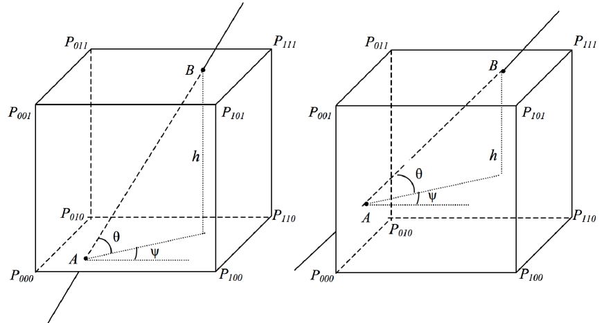
Figure 1: Two examples of the line-of-sight (lines) crossing a cubic cell of the simulation box at points $A$ and $B$. The segment $AB$ lies inside the cube. $P_{xyz}$ ($x,y,z=0,1$) are the eight vertexes of the cube. Projecting $AB$ into the plane perpendicular to $z$-direction and passing point $A$, then $\psi$ is the angle between the projection and $x$-direction, and $\theta$ is the angle between $AB$ and that plane. For the given line-of-sight and cube, $A,B,\theta,\psi$ are known or can be computed easily, and we also know the density values at the eight vertexes; we then want to integrate the density field along $AB$ (or part of it).

2.2.1 Method A

To compute the projected density field, we need to integrate along the l.o.s., and in practice this integration can be carried out progressively along the segments of lines of sight within individual cubic grid cells. The reason for such a prescription will become clear soon. Throughout this subsection we will use $z$ to denote the coordinate rather than redshift.

Fig. 1 shows two examples of such configurations, in which the part $AB$ of a line of sight lies in a grid (see the figure caption for more information). The density value at a given point on $AB$ could be computed using trilinear interpolation, as long as we know the values at the vertices, which are denoted by $\rho_{xyz}$ ($x,y,z=0,1$). To be more explicit, let us define

$$c_{0} \equiv \rho_{000},$$

$$c_{1} \equiv \rho_{100}-\rho_{000},$$

$$c_{2} \equiv \rho_{010}-\rho_{000},$$

$$c_{3} \equiv \rho_{001}-\rho_{000},$$

$$c_{4} \equiv \rho_{110}-\rho_{010}-\rho_{100}+\rho_{000},$$

$$c_{5} \equiv \rho_{011}-\rho_{001}-\rho_{010}+\rho_{000},$$

$$c_{6} \equiv \rho_{101}-\rho_{001}-\rho_{100}+\rho_{000},$$

$$c_{7} \equiv \rho_{111}-\rho_{011}-\rho_{101}-\rho_{110}$$ (11)

$$+\rho_{100}+\rho_{001}+\rho_{010}-\rho_{000}.$$

Suppose the point on $AB$ we are considering has coordinate $(x,y,z)$, then the density value is given by

$$\rho(x,y,z) = c_{0}+c_{1}\Delta x+c_{2}\Delta y+c_{3}\Delta z+c_{4}\Delta x\Delta y$$ (12)

$$+c_{5}\Delta y\Delta z+c_{6}\Delta x\Delta z+c_{7}\Delta x\Delta y\Delta z,$$

where

$$\Delta x \equiv \frac{1}{L}\left(x-x_{0}\right)\ =\ \frac{1}{L}\left[a+(\chi-\chi_{A})\cos\theta\cos\psi\right],$$

$$\Delta y \equiv \frac{1}{L}\left(y-y_{0}\right)\ =\ \frac{1}{L}\left[b+(\chi-\chi_{A})\cos\theta\sin\psi\right],$$

$$\Delta z \equiv \frac{1}{L}\left(z-z_{0}\right)\ =\ \frac{1}{L}\left[c+(\chi-\chi_{A})\sin\theta\right]$$ (13)

where $L$ denotes the size of the cubic cell, $(x_{0},y_{0},z_{0})$ is the coordinate of vertex $P_{000}$, $\chi_{A}$ is the $\chi$ value at point $A$, and $a,b,c$ are the coordinates of point $A$ relative to $P_{000}$.

Because we express $\rho(x,y,z)$ in terms of $\chi$ only, the line integral along $AB$ could be rewritten as an integral over $\chi$, and we have

$$\frac{1}{\chi_{s}}\int^{\chi_{u}}_{\chi_{l}}\chi(\chi_{s}-\chi)\rho(x,y,z)d\chi$$ (14)

$$= \frac{1}{\chi_{s}}\sum_{N=1}^{4}d_{N}\int^{\chi_{u}}_{\chi_{l}}\chi(\chi_{s}-\chi)(\chi-\chi_{A})^{N-1}d\chi$$

$$= \frac{1}{\chi_{s}}\sum_{N=1}^{4}d_{N}\int^{\tilde{\chi}_{u}}_{\tilde{\chi}_{l}}\left(\tilde{\chi}+\chi_{A}\right)\left(\chi_{s}-\chi_{A}-\tilde{\chi}\right)\tilde{\chi}^{N-1}d\tilde{\chi}$$

$$= \sum_{N=1}^{4}\frac{d_{N}}{N}\chi_{A}\left(1-\frac{\chi_{A}}{\chi_{s}}\right)\left(\tilde{\chi}^{N}_{u}-\tilde{\chi}^{N}_{l}\right)$$

$$+\sum_{N=1}^{4}\frac{d_{N}}{N+1}\left(1-2\frac{\chi_{A}}{\chi_{s}}\right)\left(\tilde{\chi}^{N+1}_{u}-\tilde{\chi}^{N+1}_{l}\right)$$

$$-\sum_{N=1}^{4}\frac{d_{N}}{N+2}\frac{1}{\chi_{s}}\left(\tilde{\chi}^{N+2}_{u}-\tilde{\chi}^{N+2}_{l}\right),$$

in which $\chi_{l}\geq\chi_{A}$ and $\chi_{u}\leq\chi_{B}$ are the lower and upper limit of the integral respectively, $\tilde{\chi}\equiv\chi-\chi_{A}$, $\tilde{\chi}_{u}\equiv\chi_{u}-\chi_{A}$, $\tilde{\chi}_{l}\equiv\chi_{l}-\chi_{A}$ and we have also defined

$$d_{1} \equiv c_{0}+\frac{1}{L}\left(ac_{1}+bc_{2}+cc_{3}\right)$$

$$+\frac{1}{L^{2}}\left(abc_{4}+bcc_{5}+acc_{6}\right)+\frac{1}{L^{3}}abcc_{7},$$

$$d_{2} \equiv \frac{1}{L}\cos\theta\cos\psi c_{1}+\frac{1}{L}\cos\theta\sin\psi c_{2}+\frac{1}{L}\sin\theta c_{3}$$

$$+\frac{1}{L^{2}}\cos\theta\sin\psi\left(ac_{4}+cc_{5}\right)$$

$$+\frac{1}{L^{2}}\cos\theta\cos\psi\left(bc_{4}+cc_{6}\right)$$

$$+\frac{1}{L^{2}}\sin\theta\left(bc_{5}+ac_{6}\right)+\frac{1}{L^{3}}\sin\theta abc_{7}$$

$$+\frac{1}{L^{3}}\cos\theta\sin\psi acc_{7}+\frac{1}{L^{3}}\cos\theta\cos\psi bcc_{7},$$

$$d_{3} \equiv \frac{1}{L^{2}}\cos^{2}\theta\sin\psi\cos\psi c_{4}+\frac{1}{L^{2}}\sin\theta\cos\theta\sin\psi c_{5}$$

$$+\frac{1}{L^{2}}\sin\theta\cos\theta\cos\psi c_{6}+\frac{1}{L^{3}}\sin\theta\cos\theta\sin\psi ac_{7}$$

$$+\frac{1}{L^{3}}\sin\theta\cos\theta\cos\psi bc_{7}$$

$$+\frac{1}{L^{3}}\cos^{2}\theta\sin\psi\cos\psi cc_{7},$$

$$d_{4} \equiv \frac{1}{L^{3}}\sin\theta\cos^{2}\theta\sin\psi\cos\psi c_{7}.$$ (15)

Note that, by writing the result in the above form, we have separated the treatments for four types of variables:

1. $a,b,c,\chi_{A},\tilde{\chi}_{u,l}$: $a,b,c,\chi_{A}$ are determined by the direction of the light ray and the specific grid cell under consideration, and $\tilde{\chi}_{u,l}$ depend only on the considered time step and $\chi_{A}$. Note that $a,b,c$ must be determined carefully, and for each grid cell at least one of them vanishes, but exactly which of them vanishes varies from ray to ray and from grid cell to grid cell;

2. $\theta,\psi$: these specify the direction of the light ray, and terms involving them only need to be computed once, i.e., at the beginning of the simulation, for a given line of sight;

3. $c_{0-7}$ – these are determined by the values of $\rho$ at the vertices of a grid, and must be evaluated for each grid that the light ray passes through;

4. $L,\chi_{s}$: these are constants for a given simulation.

Therefore once $\rho_{xyz}$ is known, the integral can be performed analytically without much computational effort. This is not unexpected, because once the density is known at the vertices of the grid, we should know the density at any point inside the grid using interpolation, and no more information is needed to carry out the integral. If we consider a different grid, a different set of $\rho_{xyz}$ needs to be used, and this is why our algorithm is based on the individual grids.

There are two technical points which need to be noted. First, in Eq. (14) $\rho$ should be replaced by $\rho/a$ in practice. It is true that $a$ could be expressed as a function of $\chi$ as well once the background cosmology is specified, but this will lead to more complicated expressions. Therefore in our simulations we simply take $a$ to be constant during each time step. This is certainly only an approximation, but we should note that $a$ is considered as constant during each time step in the $N$-body simulations anyway. Indeed, as we see in Section 2.2.2, the factor $\frac{1}{a}$ does not appear if we use $\nabla^{2}_{\xi}\Phi$ instead of $\rho$ in the integral.

Second, as has been mentioned by various papers (e.g. Jain, Seljak & White (2000); White & Hu (2000)), the use of the three dimensional Laplacian [Eq. (10)] instead of the two dimensional one [Eq. (8)] is at best an approximation. We have to test the validity of this approximation. In fact, as we show below, the error caused by this approximation is actually not negligible. To see this, recall that

$$\kappa = \int^{\chi_{s}}_{0}g\left(\nabla^{2}-\nabla^{2}_{\chi}\right)\Phi d\chi$$ (16)

$$= \frac{3}{2}\Omega_{m}H_{0}^{2}\int^{\chi_{s}}_{0}g\frac{\delta}{a}d\chi-\left[g\nabla_{\chi}\Phi\right]^{\chi_{s}}_{0}$$

$$+\int^{\chi_{s}}_{0}g\dot{\nabla}_{\chi}\Phi d\chi+\int^{\chi_{s}}_{0}g^{\prime}\nabla_{\chi}\Phi d\chi$$

in which a prime (overdot) denotes the $\chi$ (time) derivative, and the last three terms come from the treatment of $\nabla^{2}_{\chi}\Phi$, including integration by parts. The common argument is that the second term actually vanishes as $g=0$ and $\nabla_{\chi}\Phi<\infty$ at $\chi=\chi_{s}$ and $\chi=0$, and the last two terms are negligible. This is true in the ideal case, but while our algorithm [and that of White & Hu (2000)] is applied the second term is no longer zero because of the following reasons:

1. It is unrealistic to make the simulation boxes big enough to contain the whole light cone, and in practice people tile different simulations to form a complete light cone. Unless a periodic tiling of the same box is adopted, we expect the matter distribution and thus the potential $\Phi$ to be discontinuous at the tiling boundaries. As a result the second term in Eq. (16) should read

   $$\left[g\nabla_{\chi}\Phi\right]^{\chi_{s}}_{0}=\left[g\nabla_{\chi}\Phi\right]^{\chi_{s}}_{\chi_{l1}}+\left[g\nabla_{\chi}\Phi\right]^{\chi_{u2}}_{\chi_{l2}}+\cdots+\left[g\nabla_{\chi}\Phi\right]^{\chi_{uN}}_{0}$$

   in which $\chi_{u,l}$ correspond to the values of $\chi$ when the light ray goes through a given box, which is labelled as $1,2,\cdots,N$. If the matter distribution is smooth at the boundaries of the boxes, then $\nabla_{\chi}\Phi(\chi=\chi_{l1})=\nabla_{\chi}\Phi(\chi=\chi_{u2})$ and so on, so all terms cancel. However, if the matter distribution is not smooth, as is the case for many tiling treatments, then such cancelling will not happen and $\left[g\nabla_{\chi}\Phi\right]^{\chi_{s}}_{0}$ will turn out to be nonzero in the numerical calculation although it should be zero in theory.

2. Using the same argument as above, we could find that this discontinuity problem appears not only on the boundaries of the tiled simulation boxes, but also at each time-step in the simulations and each time when the light ray passes through a grid of the simulation box. For the former case, suppose that during one time step the l.o.s. ends at point $C$, then $C$ is also the point where this l.o.s. starts during the next time step. However, the values of $\nabla_{\chi}\Phi$ at point $C$ are generally different in the two time steps because particles have been advanced, and so a discontinuity appears. For the latter case, our piecewise l.o.s. integral and the interpolation scheme dictate that the values of $\nabla_{\chi}\Phi$ at a point $D$ on the interface of two neighbouring grids could depend on which grid is supposed to contain point $D$ (remember the interpolation scheme uses the values of $\nabla_{\chi}\Phi$ at the vertices of the containing cell), and naturally a discontinuity in $\nabla_{\chi}\Phi$ appears at the interface of the two grids. Note that these discontinuities are inevitable due to the nature of numerical simulation (the discreteness in time), and decreasing the grid size or the length of time steps does not help because then such discontinuities will only appear more frequently.

The way to tackle these problems is as follows: we know that $\left[g\nabla_{\chi}\Phi\right]^{\chi_{s}}_{0}$ vanishes rigorously in principle but is nonzero because of the nature of the simulation; meanwhile, the same discontinuity problem also appears when calculating the first quantity on the right-hand side of Eq. (16). The errors in the numerical values for these two quantities are caused by the same discontinuity and could cancel each other. The exact value of this error can be obtained by computing $\left[g\nabla_{\chi}\Phi\right]$, because this quantity is zero in theory and its nonzero value is completely the error. In our simulations, we compute $\left[g\nabla_{\chi}\Phi\right]$ explicitly whenever the light ray passes a grid, and subtract it according to Eq. (16): this way we can eliminate the error in the integration of $g\delta/a$ due to the discontinuities.

As for the third and fourth terms in Eq. (16), the third term is nonzero but small in reality, but in our simulations it vanishes because $\Phi$ is assumed to be constant during any given time-step. This will cause certain unavoidable errors, that we anyway expect to be small. The fourth term has as small a contribution, but fortunately we can perform the integral exactly and analytically as we have done for the first term in Eq. (16).

We have run several tests to check the accuracy of the approximations, and found the following:

1. If we simply replace the two dimensional Laplacian in Eq. (8) with a three dimensional one, as in Eq. (10), then the difference is of order 10% and even much larger for the rays for which $|\kappa|$ is small. Note that Eq. (8) can be evaluated exactly as will be described in Section 2.2.2.

2. If we explicitly calculate the term $\left[g\nabla_{\chi}\Phi\right]^{\chi_{s}}_{0}$ for each cell crossed by a ray, and subtract it according to Eq. (16), the difference between Eqs. (8, 10) is brought down to the level of 1-2%.

3. If we further include the contribution from the fourth term of Eq. (16), the difference will fall well within the percent level.

2.2.2 Method B

The method described in Section 2.2.1 is only applicable to Eq. (10), while there are also motivations for us to consider Eq. (8). For example, the use of the three-dimensional Laplacian instead of the two-dimensional Laplacian in Eq. (10) is at best an approximation and only works well on small angular scales. This is even worse in the discrete lensing approximation, because the photons of equal distance from the observer are certainly not in a plane but on a spherical shell, and this has motivated more accurate treatments such as the prescription proposed by Vale & White (2003). As another example, within the current framework the shear is not computed directly but from its relation with $\kappa$. There is certainly no problem with this, but it will be even better if we can compute $\gamma_{1,2}$ directly and compare with the results obtained from $\kappa$.

Our generalised treatment here is quite simple, taking advantage of the fact that the particle-mesh codes also give us the values of $\Phi(\mathbf{x})$ and (if necessary) $\nabla_{i}\nabla_{j}\Phi$ at the regular grid points. For simplicity, let us assume that (1) the central line of sight is parallel to the $x$-axis, and (2) the opening of the lines-of-sight bundle is a square with its sides parallel to $y,z$-axes respectively. In the two-dimensional plane perpendicular to the line of sight, the $i=1,2$ directions are set to be longitude and latitude respectively. We also define

$$\mu \equiv \nabla_{x}\nabla_{x}\Phi,$$

$$\nu \equiv \nabla_{y}\nabla_{y}\Phi,$$

$$\eta \equiv \nabla_{z}\nabla_{z}\Phi,$$

$$\zeta \equiv \nabla_{x}\nabla_{y}\Phi\ =\ \nabla_{y}\nabla_{x}\Phi,$$

$$\omega \equiv \nabla_{y}\nabla_{z}\Phi\ =\ \nabla_{z}\nabla_{y}\Phi,$$

$$\varpi \equiv \nabla_{x}\nabla_{z}\Phi\ =\ \nabla_{z}\nabla_{x}\Phi$$ (17)

to lighten the notation. Then, given the values of $\mu,\nu,\cdots$ at the vertices of a grid, their values at any point inside that grid can be obtained using trilinear interpolation just as we have done for $\rho$ in Section 2.2.1.

Now, for the configuration depicted in Fig. 1 we have, after some exercise of geometry,

$$\nabla_{1}\nabla_{1}\Phi = \chi^{2}\cos^{2}\theta\left(\mu\sin^{2}\psi+\nu\cos^{2}\psi-\zeta\sin 2\psi\right),$$

$$\nabla_{2}\nabla_{2}\Phi = \chi^{2}\left(\mu\cos^{2}\psi\sin^{2}\theta+\nu\sin^{2}\psi\sin^{2}\theta+\eta\cos^{2}\theta\right)$$

$$+\chi^{2}\zeta\sin 2\psi\sin^{2}\theta-\chi^{2}\varpi\cos\psi\sin 2\theta$$

$$-\chi^{2}\omega\sin\psi\sin 2\theta,$$

$$\nabla_{1}\nabla_{2}\Phi = \frac{1}{2}\chi^{2}\sin 2\theta\left[\frac{1}{2}(\nu-\mu)\sin 2\psi+\zeta\cos 2\psi\right]$$

$$+\chi^{2}\cos^{2}\theta\left(\varpi\sin\psi-\omega\cos\psi\right),$$

$$\nabla_{\chi}\nabla_{\chi}\Phi = \mu\cos^{2}\psi\cos^{2}\theta+\nu\sin^{2}\psi\cos^{2}\theta+\eta\sin^{2}\theta$$ (18)

$$+\zeta\sin 2\psi\cos^{2}\theta+\varpi\cos\psi\sin 2\theta$$

$$+\omega\sin\psi\sin 2\theta.$$

Note that the above expressions are all linear in $\mu,\nu,\cdots$, making the situation quite simple. As an example, for $\nabla^{2}_{\xi}\Phi=\nabla^{1}\nabla_{1}\Phi+\nabla^{2}\nabla_{2}\Phi$ we have

$$\nabla^{2}_{\xi}\Phi = \left(\sin^{2}\psi+\cos^{2}\psi\sin^{2}\theta\right)\mu$$

$$+\left(\cos^{2}\psi+\sin^{2}\psi\sin^{2}\theta\right)\nu+\eta\cos^{2}\theta$$

$$-\zeta\sin 2\psi\cos^{2}\theta-\varpi\cos\psi\sin 2\theta-\omega\sin\psi\sin 2\theta,$$

as is consistent with Castro, Heavens & Kitching (2005), and because $\psi,\theta$ are constants for a given ray

$$\int^{\chi_{s}}_{0}\frac{\chi(\chi_{s}-\chi)}{\chi_{s}}\nabla^{2}_{\xi}\Phi d\chi$$ (19)

$$= \left(\sin^{2}\psi+\cos^{2}\psi\sin^{2}\theta\right)\langle\mu\rangle-\langle\zeta\rangle\sin 2\psi\cos^{2}\theta$$

$$+\left(\cos^{2}\psi+\sin^{2}\psi\sin^{2}\theta\right)\langle\nu\rangle+\langle\eta\rangle\cos^{2}\theta$$

$$-\langle\varpi\rangle\cos\psi\sin 2\theta-\langle\omega\rangle\sin\psi\sin 2\theta,$$

where

$$\langle\mu\rangle \equiv \int^{\chi_{s}}_{0}\frac{\chi(\chi_{s}-\chi)}{\chi_{s}}\mu d\chi$$ (20)

(and similarly $\langle\nu\rangle,\cdots$) are computed exactly as in Eq. (14). Note that we only need to compute $\langle\mu\rangle,\cdots$ during the $N$-body simulations and multiply appropriate coefficients as in Eq. (19) to obtain $\kappa$ finally. The components of the shear field $(\gamma_{1},\gamma_{2})$ could be computed using the same formula as Eq. (19), but with $\nabla_{\xi}^{2}\Phi$ replaced with $\nabla^{1}_{\ 1}\Phi-\nabla^{2}_{\ 2}\Phi$ and $\nabla^{1}_{\ 2}\Phi$ correspondingly using the expressions given in Eq. (2.2.2).

Figure 2: Plotted is the $\Delta^{2}_{m}(k)\equiv k^{3}P(k)/\left(2\pi^{2}\right)$, in which $P(k)$ is the matter power spectrum, as a function of the wavenumber $k$ in units of $h$ Mpc^-1. The symbols with error bars represent averaged results at $z=0$ from 10 realisations for the $B=80h^{-1}$ Mpc simulations. The solid curve is the corresponding result using the Smith et al. (2003) fit and the same set of cosmological parameters.

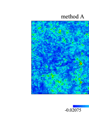
Figure 3: Convergence and shear maps ($5^{\circ}\times 5^{\circ}$) for one realisation from the tiling solutions. The convergence field $\kappa$ is shown as a colour-scale plot and the values are indicated by the colour bar below; the shear field $(\gamma_{1},\gamma_{2})$ is shown as a flow plot and superposed on the $\kappa$ field for comparison. As expected, the shear field is tangential around high-$\kappa$ regions. Note that: (1) the $\kappa$ field in the left panel is computed according to Eq. (16) with the last three correction terms incorporated as described in Section 2.2.1; (2) the $\kappa$ field in the right panel is computed using Eq. (19); (3) the $(\gamma_{1},\gamma_{2})$ field in the left panel is computed using Eq. (19) but with $\nabla_{\perp}^{2}\Phi$ replaced by $\nabla_{1}^{2}\Phi-\nabla_{2}^{2}\Phi$ (for $\gamma_{1}$) and $\nabla_{1}\nabla_{2}\Phi$ (for $\gamma_{2}$); (4) the $(\gamma_{1},\gamma_{2})$ field in the right panel is computed indirectly by Fourier transforming $\kappa(\vec{\theta})$ to $\tilde{\kappa}(\mathbf{l})$, computing $(\tilde{\gamma}_{1},\tilde{\gamma}_{2})=\left(\frac{l_{1}^{2}-l_{2}^{2}}{l_{1}^{2}+l_{2}^{2}}\tilde{\kappa},\frac{2l_{1}l_{2}}{l_{1}^{2}+l_{2}^{2}}\tilde{\kappa}\right)$ and finally inverse Fourier transforming $(\tilde{\gamma}_{1},\tilde{\gamma}_{2})$ to $(\gamma_{1},\gamma_{2})$.

3 $N$-body and Ray-tracing Simulations

To test our algorithm, we have performed a series of $N$-body simulations for a concordance cosmology using the publicly available code MLAPM (Knebe, Green & Binney, 2001). As it is not our intention to carry out very high-resolution simulations here, we only use the particle-mesh part of MLAPM so that our simulation grid is not self-adaptively refined. We have also developed a C code, RATANA (which stands for ANAlytic RAy-Tracing), to compute the convergence and shear fields on-the-fly as described in the above section. This section is devoted to a summary of our results.

3.1 Specifications for $N$-body Simulations

We consider a concordance cosmology with cosmological parameters $\Omega_{m}=0.257$, $\Omega_{\Lambda}=0.743$, $h\equiv H_{0}/(100~{}\mathrm{km/s/Mpc})=0.719$, $n_{s}=0.963$ and $\sigma_{8}=0.769$. The simulations start at an initial redshift $z_{i}=49.0$, and initial conditions (i.e., initial displacements and velocities of particles) are generated using GRAFIC (Bertschinger, 1995). In this work we only consider a source redshift $z_{s}=1.0$, though other values of $z_{s}$ or even multiple source redshifts can easily be implemented. The field-of-view is $5^{\circ}\times 5^{\circ}$, and we trace $1024^{2}$ light rays.

A source at redshift $z_{s}=1.0$ is about $2374h^{-1}$ Mpc away from us ($z=0$) in terms of comoving angular diameter distance, and it is unrealistic for us to have a simulation box which is large enough to cover the whole light-cone. In this work we adopt the tiling scheme introduced by White & Hu (2000). They use multiple simulation boxes to cover the light-cone between $z=0$ and $z_{s}$, and the sizes of the simulation boxes are adjusted so that smaller boxes are used as the light rays get closer to the observer. It has been argued that the use of multiple tiling boxes can compensate the lack of statistical independence of fluctuations caused by using the same simulation box repeatedly. Also the variable box sizes mean that one can get better angular resolutions by using smaller boxes near the observer.

Similar to White & Hu (2000), we choose six different box-sizes and 20 tiles between $z=0$ and $z_{s}$, and the details are summarised in Table 1. For the $N$-body simulations (regardless of the box sizes), we use a regular mesh with $512\times 512\times 512$ cubic cells. We use the triangular-shaped cloud (TSC) scheme to assign the matter densities in the grid cell, and to interpolate the forces (Hockney & Eastwood, 1981; Knebe, Green & Binney, 2001). Given the matter densities in the cells, the gravitational potential $\Phi$ is computed using fast Fourier transform (FFT), and the gravitational forces (first derivatives of $\Phi$) as well as the second derivatives of $\Phi$ are then obtained by performing finite differences. These derivatives of $\Phi$ are subsequently utilised by RATANA to compute the convergence and shear fields as described in the above section.

Table 1: The tiling solution of our $N$-body simulations. Here $a_{\mathrm{out}}$ is the scale factor at the time when the light rays which are traced leave a given tile, and $B$ is the size of the simulation box in units of $h^{-1}$ Mpc. Each simulation uses exactly 400 time steps from $z=49$ to $z=0$. $N_{\mathrm{real}}$ is the number of realisations for each value of box size. To obtain a tiling solution we randomly pick out two different simulation boxes with $B=240$, two with $B=200$, two with $B=160$, two with $B=120$, two with $B=100$ and 10 with $B=80$ – a total of 20 simulation boxes of different sizes.

$a_{\mathrm{out}}$	$B(h^{-1}~{}\mathrm{Mpc})$	$N_{\mathrm{real}}$	$a_{\mathrm{out}}$	$B(h^{-1}~{}\mathrm{Mpc})$	$N_{\mathrm{real}}$
$0.527$	$240$	$10$	$0.799$	$80$	$20$
$0.561$	$240$	$-$	$0.819$	$80$	$-$
$0.593$	$200$	$10$	$0.838$	$80$	$-$
$0.628$	$200$	$-$	$0.860$	$80$	$-$
$0.657$	$160$	$10$	$0.880$	$80$	$-$
$0.686$	$160$	$-$	$0.902$	$80$	$-$
$0.711$	$120$	$10$	$0.927$	$80$	$-$
$0.735$	$120$	$-$	$0.951$	$80$	$-$
$0.757$	$100$	$10$	$0.976$	$80$	$-$
$0.780$	$100$	$-$	$1.000$	$80$	$-$

Note that unlike in many other works, we use the same grid for both $N$-body and ray-tracing simulations. The TSC scheme we are using then results in some small-scale details of the matter distribution being smoothed out, as compared to the conventional nearest grid point (NGP) or cloud-in-cell (CIC) density-assignment schemes. We will comment on this point later.

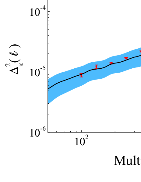
Figure 4: The convergence power spectrum $\Delta^{2}_{\kappa}\equiv l^{2}C_{l}/(2\pi)$ as measured from our ray-tracing simulations (symbols with error bars). The result is obtained by averaging 120 realisations of the tiling solution. The solid curve is again obtained using the Smith et al. (2003) fit of the matter power spectrum (Kaiser, 1992; Jain & Seljak, 1997), and the filled band illustrates the expected observational uncertainty from DES.

3.2 Numerical Results

In this subsection we summarise the numerical results from our $N$-body and ray-tracing simulations.

In Fig. 2 we compare the matter power spectra (or equivalently $\Delta^{2}_{m}(k)$ defined in the figure caption) computed from our $N$-body simulations (box size 80$h^{-1}$ Mpc) to the prediction of the analytic fitting formula of Smith et al. (2003). We can see a good agreement, except in the range of $0.5h~{}\mathrm{Mpc}^{-1}\leq k\leq 2.0h~{}\mathrm{Mpc}^{-1}$ where the $N$-body simulations predict a slightly higher power. However, the agreement becomes poor for $k>5.0h~{}\mathrm{Mpc}^{-1}$ because the resolution of our simulations is not high enough, but this could be overcome in future higher-resolution simulations.

To show that our ray-tracing simulations produce reasonable results, we first consider the convergence and shear maps from a chosen realisation of tiling solution, and these are shown in Fig. 3. We have computed the convergence field $\kappa(\vec{\xi})$, using the two methods outlined in Sections 2.2.1 (Method A, Eq. (16), left panel of Fig. 3) and 2.2.2 (Method B, Eq. (19), right panel of Fig. 3). The two methods give almost identical results, and as we have checked, the difference is in general well within the percent level. The shear field $\left(\gamma_{1},\gamma_{2}\right)$ is also calculated using two methods: method A using an equivalence of Eq. (19) as described in the figure caption (left panel), and method B which is often used in the literature, namely by Fourier transforms of the convergence field which only works in the weak-lensing regime (right panel). The shear fields are shown in rods along with the convergence map shown as images. Again, the agreement for the shear field is very good, indicating that our ray-tracing algorithm works well.

We also show the lensing convergence power spectrum measured from our ray-tracing simulations in Fig. 4. Due to our limit field of view of $(5^{\circ}\times 5^{\circ})$, we cannot measure the spectrum at multiple moment $\ell<100$. Also, there is a rolloff of power at $\ell>2000$, which is because (1) the resolution for our $N$-body simulations is not high enough and (2) the TSC density-assignment scheme smooths out the small-scale structure more than the CIC and NGP schemes do. Both factors tend to suppress the convergence power spectrum at high $\ell$ and we hope to solve this problem by using higher resolution simulations and more suitable interpolation schemes, which is left for our future study. Otherwise, we find that the ray-tracing result agrees reasonably well with the analytic prediction using the fitting formula for matter power spectrum by Smith et al. (2003) in some $\ell$ range, i.e., $100<\ell<2000$. On some scales, we see that the numerical result is slightly higher than the theoretical prediction. This is however as expected because we have seen from Fig. 2 that the $N$-body simulations give a higher matter power spectrum than the Smith et al. (2003) fit on some scales. The fact that a difference in the matter power spectra from simulations and analytic fitting could cause differences in the computed convergence power spectra has been reported and discussed by many authors, e.g., Vale & White (2003); Hilbert et al. (2009); Pielorz et al. (2010). In Fig. 4, we overplot the expected observational uncertainty from DES using the survey parameters $f_{\rm sky}\sim 0.12,\bar{n}_{\rm g}=10$/arcmin², $\gamma_{\rm int}^{2}\sim 0.16$ where $f_{\rm sky},\bar{n}_{\rm g}$ and $\gamma_{\rm int}^{2}$ denote the sky coverage, number of galaxies per arc-minute squared and the mean-square intrinsic ellipticity, respectively.

Note that in our numerical simulations we have not included the lens-lens coupling and second-order corrections to the Born approximation. In Appendix A we will outline how these can be incorporated in future higher-resolution simulations.

4 Discussion and Conclusion

The correlations in the distorted images of distant galaxies, induced by cosmic shear, hold information about the distribution of matter on a wide range of scales in the universe. In order to take full advantage of current and future weak lensing data sets to constrain cosmology, using information from both the linear and non-linear regimes, one needs a sophisticated algorithm to measure the shear and convergence fields from $N$-body simulations, and to construct statistical quantities. This is traditionally done using the ‘plane-by-plane’ discrete lens-plane algorithm – trace the virtual light rays and calculate the deflection caused by the density field projected onto a number of 2-D lensing planes.

In this work, we propose an improved ray-tracing algorithm. We calculate the deflection of the light rays caused by the detailed 3-D density fields living on the natural simulation mesh, rather than the simplified density distribution projected onto some 2-D planes. We evaluate the shear and convergence fields by analytically integrating the deflection as the light rays go through the individual simulation grid cells. This approach is easy to implement and computationally inexpensive. It avoids numerical integration, and expensive data storage since it is performed on the fly. We apply the algorithm to our simulations, and find good agreement with the Smith et al. (2003) fit, and consistency with the published results in Sato et al. (2009).

The on-the-fly l.o.s. integration is computationally economic. In the RATANA code, most computation time is spent on the $N$-body part. Suppose $N_{d}^{3}$ is the number of grid cells in our mesh, then the FFT requires $3N_{d}^{3}\log_{2}N_{d}$ operations each time step, not including other operations such as differencing the potential to obtain the force on the mesh, assigning particles and computing densities on all the grid cells and particle movements. In contrast, if we let $N_{\rm{los}}=N_{d}$ (which is enough for accuracy), then there are only $N_{d}^{2}$ rays to trace, and for each ray we have $\leq 10^{2}$ operations. We have checked the simulation log file and found that there is no significant difference in the times used by each step before and after the ray-tracing part of RATANA has been triggered.

Analytic formulae are often more useful than purely numerical results in tracing the physical contents of a theory. For example, in Eqs. (14, 2.2.1), it is easy to check which terms contribute the most to the final result: obviously, in the small-angle limit, i.e., $\theta,\psi\ll 1$, terms involving $d_{3},d_{4}$, and a large part of $d_{2}$ could be neglected because $\sin\theta,\sin\psi\ll 1$; also at least one of $a,b,c$ vanishes and $abc=0$ for all grid cells, further simplifying $d_{1},d_{2}$; furthermore, terms in Eq. (14) with coefficient $1/\chi_{s}$ contribute little because $\chi_{s}\gg\tilde{\chi}_{u,l}$. Such observations can be helpful in determining which terms have important effects in certain regimes.

Note that the dependence on $\chi_{s}$ [cf. Eq. (14)] could be taken out of the analytical integration, meaning that the algorithm can be straightforwardly generalised to include multiple source redshifts with very little extra computational effort (mainly in determining where to start the integration for a given source redshift). The algorithm can also be easily generalised to compute the flexion, which depends on higher-order derivatives of the lensing potential, and is expected to give more accurate results than the multiple-lens-plane approximation.

The algorithm has many other flexibilities too. As an example, the analytic integration of the projected density and potential fields along the l.o.s. can be performed on an adaptive rather than a regular grid with careful programming, which means that higher resolution can be achieved in high density regions, as in the adaptive PM simulations. Also, the analytic integration can be easily generalised to other algorithms to compute the 3-D shear field (Couchman, Barber & Thomas, 1999).

We also give prescriptions to include second-order corrections to the results, such as the lens-lens coupling and corrections to the Born approximation, in Appendix A. It is interesting to note that, by running the $N$-body simulations backwards in time, we can still compute the convergence and shear fields on-the-fly even if the light rays are not straight.

To conclude, the algorithm described here is efficient and accurate, and is suitable for the future ray-tracing simulations using very large $N$-body simulations. It will be interesting to apply it to study the higher-order statistics of the shear field and the lensing excursion angles, and these will be left for future work.

Appendix A Beyond the First-order Approximations

In the attempt to trace light rays on the fly, we set up a bundle of l.o.s. before the $N$-body simulation starts. But because we do not know the exact paths of those light rays which finally end up at the observer, we have to assume that they are straight lines even though they are not in reality. This so-called Born approximation is generally quite good in the weak lensing regime, but can lead to non-negligible errors on small scales (Hilbert et al., 2009). Furthermore, in the above treatment we have also neglected the lens-lens coupling, which accounts for the fact that the lenses themselves (the large-scale structure) are distorted by the lower-redshift matter distribution.

Hilbert et al. (2009) take account of the lens-lens coupling and corrections to the Born approximation using the multiple-lens-plane approximation. In such an approach, the light rays get deflected and their paths are recomputed when and only when they pass by a discrete lens plane.

Since our algorithm goes beyond the discrete lens-plane approximation and is able to trace the detailed matter distribution, we want to generalise it to include those corrections as well. In this Appendix we shall derive an analytical formula for the distortion matrix with the lens-lens coupling taken into account, and describe how the corrections to the Born approximation can be incorporated as well.

Obviously, to go beyond the Born approximation, the light rays are no longer straight and thus the l.o.s cannot be set up before the $N$-body simulation has finished. Instead, we have to start from the observer today and go backwards in time to compute the distortion matrix Eq. (3). We shall discuss below how this could be realised in practice, but at this moment let us simply assume that we can go backwards in time, and know the value of the lensing potential $\Phi$ and its derivatives along the l.o.s..

A.1 Corrections to the Born Approximation

The corrections to the Born approximation are easy to implement. According to Eq. (2), the total deflection of a light ray is the sum of the deflections by the matter in each grid that ray passes on its way towards the lensing source. Suppose $\vec{\xi}^{(n)}$ denotes the value of $\vec{\xi}$ after the light ray crosses the $n$-th grid on its way ($n$ increases with the distance from the observer, $n=1$ corresponds to the grid which the observer is in, and $\vec{\xi}^{(0)}=\vec{\xi}_{0}$), then

$$\vec{\xi}^{(n)} = \vec{\xi}^{(n-1)}-2\int^{\chi^{(n)}_{u}}_{\chi^{(n)}_{l}}\frac{\chi_{s}-\chi}{\chi\chi_{s}}\vec{\nabla}_{\vec{\xi}}\Phi d\chi,$$ (21)

where $\chi^{(n)}_{u}\equiv\min\left\{\chi^{\mathrm{ts}}_{u},\chi^{(n)}_{B}\right\}$ and $\chi^{(n)}_{l}\equiv\max\left\{\chi^{\mathrm{ts}}_{l},\chi^{(n)}_{A}\right\}$, in which $\chi^{\mathrm{ts}}_{u}>\chi^{\mathrm{ts}}_{l}$ are respectively the $\chi$-values at the two ends of the current time step, and $\chi^{(n)}_{B}>\chi^{(n)}_{A}$ the $\chi$-values of the two intersections between the light ray and the $n$-th grid. Using the expressions given in Sect. 2.2.2, it is easy to write $\nabla_{\xi_{1}}\Phi$ and $\nabla_{\xi_{2}}\Phi$ in terms of polynomials of $\chi$. Then the above integral can be performed analytically as before. In this way, each time the light ray crosses a grid, we update its orientation according to the above equation, and thus the corrections to the Born approximation can be incorporated.

Note that in this approach the light rays are deflected many more times than in the multiple-lens-plane approximation and the detailed matter distribution has been fully taken account of.

A.2 Lens-lens Coupling

As mentioned earlier, the lens-lens coupling has been neglected in the above treatment because in Eq. (3) we have used the approximation $\nabla_{\chi_{0i}}\approx\nabla_{\chi_{i}}$. Let us now have a look at what happens when this approximation is dropped.

Note that in the expression

$$A_{ij} \equiv -2\int^{\chi_{s}}_{0}\frac{g(\chi,\chi_{s})}{\chi^{2}}\nabla_{\xi_{0i}}\nabla_{\xi_{j}}\Phi\left(\chi,\vec{\xi}\right)d\chi+\delta_{ij},$$ (22)

the argument of $\Phi$ is $\vec{\xi}$ while one of the derivatives is with respect to $\vec{\xi}_{0}$. We can utilise the chain rule to write $\nabla_{\xi_{0i}}=\left(\nabla_{\xi_{0i}}\xi_{j}\right)\nabla_{\xi_{j}}=A_{ij}\nabla_{\xi_{j}}$ where we have used the definition of $A_{ij}$ given in Sect. 2.1. Then the above equation becomes

$$A^{i}_{\ j}\left(\chi_{s},\vec{\xi}\right) \equiv \delta^{i}_{\ j}-2\int^{\chi_{s}}_{0}g(\chi,\chi_{s})\nabla^{i}\nabla_{k}\Phi\left(\chi,\vec{\xi}\right)A^{k}_{\ j}\left(\chi,\vec{\xi}\right)d\chi,$$ (23)

where for simplicity we have used $\nabla_{i}=\nabla_{\xi_{i}}$. With the $A^{k}_{\ j}$ term in the integrand, Eq. (23) now includes the lens-lens coupling, and will be our starting point here.

Again, let us consider the integral in Eq. (23) after the light ray crosses the $n$-th grid on its way towards the lensing source. The discrete version of Eq. (23) is

$${}^{(n)}A^{i}_{\ j} = {}^{(n-1)}A^{i}_{\ j}-2\int^{\chi^{(n)}_{u}}_{\chi^{(n)}_{l}}\frac{\chi\left(\chi_{s}-\chi\right)}{\chi_{s}}~{}^{(n)}A^{k}_{\ j}\nabla^{i}\nabla_{k}\Phi d\chi$$ (24)

where ${}^{(n)}A^{i}_{\ j}$ is the value of $A^{i}_{\ j}$ after the light ray has crossed the $n$-th grid, and ${}^{(0)}A^{i}_{\ j}=\delta^{i}_{\ j}$ as is easy to see. This formula has three advantages as compared to the multiple-lens-plane approximation:

1. As before, the light rays between $z=0$ and $z_{s}$ are divided into many more segments, and the fine structure of the matter distribution is included naturally, without squeezing the matter and using impulse approximations.

2. As will be shown below, the integration can be evaluated analytically rather than numerically.

3. Note that we can use ${}^{(n)}A^{k}_{\ j}$ rather than ${}^{(n-1)}A^{k}_{\ j}$ in the integrand, which will give more accurate results, because using ${}^{(n-1)}A^{k}_{\ j}$ would mean that the contribution to the lens-lens coupling from the matter in the $n$-th grid is ignored. In the multiple-lens-plane approximation which typically uses $20\sim 30$ lens planes, the $n$-th plane could contain a significant amount of matter, and neglecting its contribution could make the results less accurate.

Eq. (24) is exact, but we only want the result to second order in $\nabla\nabla\Phi$. Therefore we can iterate once and write an approximate solution as

$${}^{(n)}A^{i}_{\ j} \approx {}^{(n-1)}A^{i}_{\ j}-2~{}^{(n-1)}A^{k}_{\ j}\int^{\chi^{(n)}_{u}}_{\chi^{(n)}_{l}}d\chi\frac{\chi\left(\chi_{s}-\chi\right)}{\chi_{s}}\nabla^{i}\nabla_{k}\Phi$$

$$+4\int^{\chi^{(n)}_{u}}_{\chi^{(n)}_{l}}d\chi\frac{\chi\left(\chi_{s}-\chi\right)}{\chi_{s}}\nabla^{i}\nabla_{k}\Phi\left(\chi,\vec{\xi}\right)\int^{\chi}_{\chi^{(n)}_{l}}d\chi^{\prime}\frac{\chi^{\prime}\left(\chi-\chi^{\prime}\right)}{\chi}\nabla^{k}\nabla_{j}\Phi\left(\chi^{\prime},\vec{\xi}\right).$$

Following the approach taken in Sect. 2.2.1 we can write

$$\nabla^{i}\nabla_{j}\Phi\left(\chi,\vec{\xi}\right) = \sum_{N=1}^{4}\left(\mathbf{K}_{N}\right)^{i}_{\ j}\left(\chi-\chi_{A}^{(n)}\right)^{N-1},$$ (26)

where $\chi_{A}^{(n)}$ is defined in Eq. (21), and $\mathbf{K}_{N}$ ($N\in\{1,2,3,4\}$) is a $2\times 2$ matrix whose $ij$-component depends on the orientation of the l.o.s. segment inside the $n$-th grid (where it is taken to be straight) and the values of $\nabla^{i}\nabla_{j}\Phi$ at the vertices of the $n$-th grid. Note however that $\mathbf{K}_{N}$ is independent of $\chi$. The expressions are similar to the $d_{N}$s defined in Sect. 2.2.1 and we shall not write them explicitly here.

Substituting Eq. (26) into Eq. (A.2), we find

$${}^{(n)}A^{i}_{\ j} = ~{}^{(n-1)}A^{i}_{\ j}-2\sum^{4}_{N=1}I_{1}(N)\left(\mathbf{K}_{N}\right)^{i}_{\ k}~{}^{(n-1)}A^{k}_{\ j}+4\sum^{4}_{N=1}\sum^{4}_{M=1}I_{2}(N,M)\left(\mathbf{K}_{N}\right)^{i}_{\ k}\left(\mathbf{K}_{M}\right)^{k}_{\ j}$$ (27)

in which we have written (again, by defining $\tilde{\chi}\equiv\chi-\chi_{A}^{(n)}$, $\tilde{\chi}^{\prime}\equiv\chi^{\prime}-\chi_{A}^{(n)}$ and $\tilde{\chi}^{(n)}_{u,l}\equiv\chi^{(n)}_{u,l}-\chi_{A}^{(n)}$)

$$I_{1}(N) \equiv \int^{\chi^{(n)}_{u}}_{\chi^{(n)}_{l}}d\chi\frac{\chi\left(\chi_{s}-\chi\right)}{\chi_{s}}\left(\chi-\chi_{A}^{(n)}\right)^{N-1}$$ (28)

$$= \frac{1}{N}\chi_{A}^{(n)}\left(1-\frac{\chi^{(n)}_{A}}{\chi_{s}}\right)\left[\left(\tilde{\chi}^{(n)}_{u}\right)^{N}-\left(\tilde{\chi}^{(n)}_{l}\right)^{N}\right]+\frac{1}{N+1}\left(1-\frac{2\chi^{(n)}_{A}}{\chi_{s}}\right)\left[\left(\tilde{\chi}^{(n)}_{u}\right)^{N+1}-\left(\tilde{\chi}^{(n)}_{l}\right)^{N+1}\right]$$

$$-\frac{1}{N+2}\frac{1}{\chi_{s}}\left[\left(\tilde{\chi}^{(n)}_{u}\right)^{N+2}-\left(\tilde{\chi}^{(n)}_{l}\right)^{N+2}\right],$$

and

$$I_{2}(N,M) \equiv \int^{\chi^{(n)}_{u}}_{\chi^{(n)}_{l}}d\chi\frac{\chi_{s}-\chi}{\chi_{s}}\left(\chi-\chi_{A}^{(n)}\right)^{N-1}\int^{\chi}_{\chi^{(n)}_{l}}d\chi^{\prime}\chi^{\prime}(\chi-\chi^{\prime})\left(\chi^{\prime}-\chi_{A}^{(n)}\right)^{M-1}$$ (29)

$$= -\frac{\left(\tilde{\chi}^{(n)}_{u}\right)^{M+N+3}-\left(\tilde{\chi}^{(n)}_{l}\right)^{M+N+3}}{(M+1)(M+2)(M+N+3)}\frac{1}{\chi_{s}}+\frac{\left(\tilde{\chi}^{(n)}_{u}\right)^{M+N+2}-\left(\tilde{\chi}^{(n)}_{l}\right)^{M+N+2}}{(M+1)(M+2)(M+N+2)}\left(1-\frac{\chi_{A}^{(n)}}{\chi_{s}}\right)$$

$$-\frac{\left(\tilde{\chi}^{(n)}_{u}\right)^{M+N+2}-\left(\tilde{\chi}^{(n)}_{l}\right)^{M+N+2}}{M(M+1)(M+N+2)}\frac{\chi_{A}^{(n)}}{\chi_{s}}+\frac{\left(\tilde{\chi}^{(n)}_{u}\right)^{M+N+1}-\left(\tilde{\chi}^{(n)}_{l}\right)^{M+N+1}}{M(M+1)(M+N+1)}\chi_{A}^{(n)}\left(1-\frac{\chi_{A}^{(n)}}{\chi_{s}}\right)$$

$$+\left[\frac{1}{M}\frac{\chi_{A}^{(n)}}{\chi_{s}}+\frac{1}{M+1}\frac{\chi_{l}^{(n)}}{\chi_{s}}\right]\left(\chi_{l}^{(n)}\right)^{M}\frac{1}{N+2}\left[\left(\tilde{\chi}^{(n)}_{u}\right)^{N+2}-\left(\tilde{\chi}^{(n)}_{l}\right)^{N+2}\right]$$

$$-\left(1-\frac{\chi_{A}^{(n)}}{\chi_{s}}\right)\left[\frac{1}{M}\chi_{A}^{(n)}+\frac{1}{M+1}\chi_{l}^{(n)}\right]\left(\chi_{l}^{(n)}\right)^{M}\frac{1}{N+1}\left[\left(\tilde{\chi}^{(n)}_{u}\right)^{N+1}-\left(\tilde{\chi}^{(n)}_{l}\right)^{N+1}\right]$$

$$-\left[\frac{1}{M+1}\frac{\chi_{A}^{(n)}}{\chi_{s}}+\frac{1}{M+2}\frac{\chi_{l}^{(n)}}{\chi_{s}}\right]\left(\chi_{l}^{(n)}\right)^{M+1}\frac{1}{N+1}\left[\left(\tilde{\chi}^{(n)}_{u}\right)^{N+1}-\left(\tilde{\chi}^{(n)}_{l}\right)^{N+1}\right]$$

$$+\left(1-\frac{\chi_{A}^{(n)}}{\chi_{s}}\right)\left[\frac{1}{M+1}\chi_{A}^{(n)}+\frac{1}{M+2}\chi_{l}^{(n)}\right]\left(\chi_{l}^{(n)}\right)^{M+1}\frac{1}{N}\left[\left(\tilde{\chi}^{(n)}_{u}\right)^{N}-\left(\tilde{\chi}^{(n)}_{l}\right)^{N}\right].$$

The above expressions look rather heavy, however, they are analytic and as a result are very easy to implement in the ray-tracing simulation codes, by writing functions that take $M,N,\chi_{A}^{(n)},\chi_{u}^{(n)},\chi_{l}^{(n)}$ as parameters and return $I_{1},I_{2}$ as outputs. Furthermore, since the grid size ($<0.2h^{-1}$ Mpc) in the $N$-body simulations is small enough compared with the typical inter-plane distances in the multiple-lens-plane approximations ($10\sim 100h^{-1}$ Mpc), we can drop the $I_{2}(N,M)$ terms to a very good approximation, which will greatly simplify the results.

Note that the distortion matrix $A^{i}_{\ j}$ computed in this way is not symmetric because of the matrix multiplications. However, using Eq. (7), it is straightforward to compute $\gamma_{2}=-\left(A^{1}_{\ 2}+A^{2}_{\ 1}\right)/2$. In addition, we could also calculate the rotation $\omega$ as $\omega=\left(A^{2}_{\ 1}-A^{1}_{\ 2}\right)/2$

A.3 Going Back In Time

As mentioned above, to include the actual deflections of the light rays which end up at the observer, we have to start from the observer and go backwards in time until encountering the source. This obviously can only be done after the $N$-body simulation has finished.

One way to go backwards is to record the information about the gravitational potential $\Phi$ and its derivatives in a light cone during the simulation, and then post-process the light-cone data. This means that a large amount of dump data has to be stored.

Alternatively, one can think of running the $N$-body simulation ”backwards”. To be more explicit, the simulation is first run in the forward direction from a high redshift until today, and we obtain the particle positions and velocities at present; then we reverse the directions of the gravitational force and the particle velocities, and evolve the system back until $z_{s}$ using the same time-stepping scheme as in the forward simulation. In this way, the actual light rays and distortion matrix could be built up on the fly, and there is no need to store a lot of dump data.

References

- Bacon et al (2000) Bacon, D.J., Refregier, A.R., Ellis, R.S. 2000, MNRAS, 318, 625
- Bartelmann & Schneider (2001) Bartelmann M., Schneider P., 2001, Phys. Rep., 340, 291
- Bertschinger (1995) Bertschinger E., astro-ph/9506070
- Bridle & King (2007) Bridle S., King L. J., 2007, NJPh, 9, 444
- Castro, Heavens & Kitching (2005) Castro P. G., Heavens A. F., Kitching T. D., 2005, PRD 72, 023516
- Chongchitnan & King (2010) Chongchitnan S., King L. J., 2010, MNRAS, 407, 1989
- Colombi et al (2009) Colombi S., Jaffe A., Novikov D., Pichon C., 2009, MNRAS, 393, 511
- Copland, Sami & Tsujikawa (2006) Copeland E., Sami M., Tsujikawa S., 2006, Int. J. Mod. Phys. D, 15, 1753
- Couchman, Barber & Thomas (1999) Couchman H. P. M., Barber A. J., Thomas P. A., 1999, MNRAS, 310, 453
- Crittenden, Pogosian & Zhao (2009) Crittenden R. G., Pogosian L., Zhao G. -B., JCAP 0912 (2009) 025.
- Fu et al. (2008) Fu L. et al., 2008, A & A 479, 9
- Hamana & Mellier (2001) Hamana T., Mellier Y., 2001, MNRAS, 327, 169
- Heinamaki et al. (2005) Heinamaki P., Suhhonenko I., Saar E., Einasto M., Einasto J., Virtanen H., 2005, arXiv: astro-ph/0507197
- Hilbert et al. (2009) Hilbert S., Hartlap J., White S. D. M., Schneider P., 2009, A & A 499, 31
- Hoekstra et al. (2006) Hoekstra H., Mellier Y., van Waerbeke L., Semboloni E., Fu L., Hudson M. J., Parker L. C., Tereno I., Benabed K., 2006, ApJ 647, 116
- Hockney & Eastwood (1981) Hockney R. W., Eastwood J. W., 1981, Computer Simulation Using Particles (New York: McGraw-Hill)
- Jain & Seljak (1997) Jain B., Seljak U., 1997, ApJ 484, 560
- Jain, Seljak & White (2000) Jain B., Seljak U., White S. D. M., 2000, ApJ 530, 547
- Kaiser (1992) Kaiser N., 1992, ApJ 388, 272
- Kaiser, Wilson & Luppino (2000) Kaiser N., Wilson G., Luppino G., 2000, astro-ph/0003338
- Knebe, Green & Binney (2001) Knebe A., Green A., Binney J., 2001, MNRAS, 325, 845
- Lewis & Challinor (2009) Lewis A., Challinor A., 2009, Phys. Rept., 429, 1
- Li et al. (2009) Li H., Liu J., Xia J. -Q. et al., Phys. Lett. B675 (2009) 164-169.
- Maoli et al. (2001) Maoli R., van Waerbeke L., Mellier Y., Schneider P., Jain B., Bernardeau F., Erben T., Fort B., 2001, A & A, 368, 766
- Mellier (1999) Mellier Y., 1999, A & A, 37, 127
- Pielorz et al. (2010) Pielorz J., Rodiger J., Tereno I., Schneider P., 2010, A & A 514, A79
- Sato et al. (2009) Sato M., Hamana T., Takahashi R., Takada M., Yoshida N., Matsubara T., Sugiyama N., 2009, ApJ, 701, 945
- Schmidt (2008) Schmidt F., 2008, Phys.Rev.D 78, 043002
- Schrabback et al. (2010) Schrabback T. et al., 2010, A & A 516, 63
- Smith et al. (2003) Smith R. E., Peacock J. A., Jenkins A., et al., 2003, MNRAS, 341, 1311
- Song et al. (2010) Song Y. -S., Zhao G. -B., Bacon D. et al., arXiv:1011.2106
- Tereno et al. (2009) Tereno I., Schimd C., Uzan J. -P., Kilbinger M., Vincent F.H., Fu L., 2009, A & A 500, 657
- Vale & White (2003) Vale C., White M., 2003, ApJ, 592, 699
- van Waerbeke et al. (2000) van Waerbeke L. et al., 2000, A & A 358, 30
- White & Hu (2000) White M., Hu W., 2000, ApJ, 537, 1
- Wittman et al. (2000) Wittman D.M., Tyson J.A., Kirkman D., Dell’Antonio I., Bernstein G., 2000, Nat, 405, 143
- Zhao et al. (2010) Zhao G. -B., Zhan H., Wang L., et al., arXiv:1005.3810
- Zhao et al. (2009) Zhao G. -B., Pogosian L., Silvestri A., et al., Phys. Rev. D79 (2009) 083513.
- Zhao et al. (2010a) Zhao G. -B., Pogosian L., Silvestri A., et al., Phys. Rev. Lett. 103 (2009) 241301.
- Zhao et al. (2010b) Zhao G. -B., Giannantonio T., Pogosian L., et al., Phys. Rev. D81 (2010) 103510.