Cosmological Constraints from a 31 GHz Sky Survey with the Sunyaev-Zel’dovich Array

Abstract

We present the results of a  6.1 square degree survey for clusters of galaxies via their Sunyaev-Zel’dovich (SZ) effect at 31 GHz. From late 2005 to mid 2007 the Sunyaev-Zel’dovich Array (SZA) observed four fields of roughly 1.5 square degrees each. One of the fields shows evidence for significant diffuse Galactic emission, and we therefore restrict our analysis to the remaining 4.4 square degrees. We estimate the cluster detectability for the survey using mock observations of simulations of clusters of galaxies; and determine that, at intermediate redshifts ($z\sim$0.8), the survey is 50% complete to a limiting mass (${\rm M_{200\overline{\rho}}}$) of ${\rm\sim 6.0\times 10^{14}}M_{\odot}$, with the mass limit decreasing at higher redshifts. We detect no clusters at a significance greater than 5 times the rms noise level in the maps, and place an upper limit on $\sigma_{8}$, the amplitude of mass density fluctuations on a scale of 8$h^{-1}$ Mpc, of ${\rm 0.84+0.07}$ at 95% confidence, where the uncertainty reflects calibration and systematic effects. This result is consistent with estimates from other cluster surveys and CMB anisotropy experiments.

1. Introduction

The number density of massive clusters of galaxies depends strongly on cosmology, in particular through the normalization of the matter power spectrum, and through the dependence of the volume element on the geometry of the universe. As the low-energy photons in the CMB traverse the hot (${\rm\sim 10^{8}~{}K}$) gas of a massive cluster, about 1% of the photons are inverse-Compton scattered. The result is a distortion in the CMB spectrum, the magnitude of which is proportional to the integrated pressure of the intra-cluster medium (ICM), i.e., the density of electrons along the line of the sight, weighted by the electron temperature (Sunyaev & Zel’dovich (1972, 1980); see also Birkinshaw (1999)). The SZ flux of a cluster is therefore a measure of its total thermal energy.

The change in the observed brightness of the CMB due to the SZ effect is given by

$$\frac{\Delta T_{\rm CMB}}{T_{\rm CMB}}=f(x)\int\sigma_{\rm T}n_{e}\frac{k_{B}T_{e}}{m_{e}c^{2}}dl\equiv f(x)y$$ (1)

where $T_{\rm CMB}$ is the cosmic microwave background temperature, $\sigma_{\rm T}$ is the Thomson scattering cross section, $k_{B}$ is Boltzmann’s constant, $c$ is the speed of light, $m_{e}$, $n_{e}$, $T_{e}$ are the electron mass, number density and temperature, respectively, and $f(x)$ contains the frequency dependence of the SZ effect (where ${\rm x\equiv\frac{h\nu}{k_{B}T_{CMB}}}$). Equation 1 defines the Compton $y$-parameter. The SZ effect appears as a temperature decrement at frequencies below $\approx 218~{}{\rm GHz}$, and as an increment at higher frequencies.

As seen in Equation 1, the ratio of $\Delta T/T$ is independent of the distance to the cluster. This means that the SZ effect is redshift-independent in both brightness and frequency, offering enormous potential for finding high-redshift clusters. A cluster catalog resulting from an SZ survey of uniform sensitivity has a cluster mass threshold that is only weakly dependent on redshift for $z\gtrsim 0.7$ (via the angular diameter distance). As a result, SZ cluster surveys are approximately mass-limited and therefore potentially powerful probes of cosmology (e.g., Carlstrom et al. 2002).

Experiments such as the South Pole Telescope (Ruhl et al. 2004) and the Atacama Cosmology Telescope (Fowler 2004) are surveying hundreds of square degrees of sky searching for galaxy clusters through their SZ effect. A precursor survey to those being performed by SPT and ACT was performed with the Sunyaev-Zel’dovich Array (SZA), an 8-telescope interferometer designed specifically for detecting the SZ effect towards clusters of galaxies. Over the span of two years, the SZA surveyed a small region of sky at 31 GHz. This survey has been valuable in characterizing both compact and diffuse cm-wave CMB foregrounds. It has resulted in a measurement of the power spectrum of the CMB at small scales (Sharp et al. 2010), a characterization of extragalactic compact source populations (Muchovej et al. 2010), and further evidence for large-scale dust-correlated microwave emission (Leitch et al. 2010, in prep). In this paper, we present results of the survey as they pertain to cosmological parameter estimation.

The paper is organized as follows: in §2 we describe the SZA observations, including a brief description of the instrument, data reduction and calibration, data quality tests, and foreground source extraction. We present the results of the survey in §3, followed by the calculation of the expected number of clusters in §4. In §5 we determine a constraint on $\sigma_{8}$ and systematic uncertainties associated with this analysis are presented in §6. We discuss our results in §7.

2. Observations

2.1. The Sunyaev-Zel’dovich Array

The Sunyaev-Zel’dovich Array (SZA) is an eight-element interferometer located at Caltech’s Owens Valley Radio Observatory near Big Pine, California. The observations presented in this analysis were obtained with wide-band receivers operating from 27–35 GHz. These receivers employ high-electron mobility transistor (HEMT) amplifiers (Pospieszalski et al. 1995), with characteristic receiver temperatures $T_{rx}\sim 11-20~{}{\rm K}$. Typical system temperatures, including noise due to the atmosphere, are on order 40-50 K. Six of the eight antennas are arranged in a close-packed configuration (spacings of 4.5-11.5 m), yielding 15 baselines sensitive to arcminute scales. Two outer antennas yield baselines of up to 65 m, for simultaneous detection of contaminating compact sources at a resolution of $\sim 22.5\arcsec$ (see Muchovej et al. (2007) for details of the array configuration).

This hybrid configuration was chosen to optimize surveying speed, and can be thought of as a superposition of two interferometers: the close-packed array acts as a filter for objects of arcminute extent on the sky, such as clusters of galaxies, and are used in generating short baseline maps; the longer baselines provide high-resolution sensitivity to compact sources, and provide the data for the long baseline maps. The resulting maps from the close-packed array are therefore optimally filtered for clusters of galaxies, with radio sources constrained by the outlying telescopes.

2.2. Field Selection

The SZA survey fields were selected to lie far from the plane of the Galaxy and to transit at high elevation at the OVRO site, minimizing atmospheric noise while optimizing the imaging capabilities of the array. Fields were spaced equally in Right Ascension ($\alpha$) to permit continuous observation. These constraints led to the selection of four regions ranging in declination ($\delta$) from ${\rm 25^{\circ}}$ to ${\rm 35^{\circ}}$. No consideration was given to the location of known bright radio sources or clusters of galaxies during field selection.

As the SZ effect itself provides no redshift information, the fields were also selected to make maximum use of publicly available optical survey data, from which photometric redshifts could be derived. Two of the fields were selected to overlap with regions for which optical data is available, namely the Deep Lens Survey (DLS Field F2) (Wittman et al. 2002) and the NOAO Deep Wide Field Survey (NDWFS) (Jannuzi & Dey 1999), also known as the Bootes field. Figure 1 depicts the approximate locations of the four fields on the IRAS ${\rm 100~{}\mu m}$ dust maps (Clegg 1980).

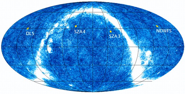
Figure 1.— IRAS dust map with overlay of the SZA field locations

.

2.3. Data Collection

Mapping large areas of sky with an interferometer requires observing multiple discrete pointings within the area to be covered, and combining the images from each pointing into a mosaic. To perform such a combination of images, each of the four fields is split into 16 rows of 16 pointings. The pointings are equally spaced by 6.6′ along great circles in the $\alpha$ direction, and each row is equally spaced by 2.9′ in the $\delta$ direction. Subsequent rows are offset from one another so that that the first pointing in each row is shifted by 3.3′ in the $\alpha$ direction relative to the previous row. This means that for a single field we observe an area that spans roughly 2 degrees in the $\alpha$ direction and 1 degree in the $\delta$ direction (see Figure 2).

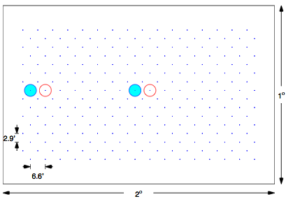
Figure 2.— Mosaic pointing locations for a given SZA survey field. The fields are divided into 16 rows of 16 columns, with the pointings in each row separated by 6.6′ and each row offset from each other by 2.9′. This leads to each field being roughly 2 degrees by 1 degree in area. In a single track the SZA observed four pointings within a given row. For example, pointings in the first and ninth, followed by pointings in the second and tenth columns.

For each of the survey fields, data were taken daily in 6 hour tracks. In a single track, we observed two staggered pairs of pointings, within a single row. These observations were performed in a manner that permits ground subtraction from consecutive pointings in a pair (although the ground contamination was found to be negligible and was not subtracted as part of the analysis of this paper). Each track results in roughly 1 hour of observation on each of the four pointings, with very nearly the same Fourier sampling for pairs of pointings. A second track is run at a later date, with the order of the pairs reversed, to ensure that the Fourier sampling for all four pointings is comparable. In Figure 2 we show the position of the pointings in each field, and indicate how the pointings were observed in a given track.

For each set of four pointings, this sequence is repeated three times over the span of roughly one year, so that each pointing is observed in six tracks, translating to roughly 6 hours of observation per pointing over the duration of the survey.

2.4. Observations and Data Reduction

Table 1Survey Observations

Field Name	Field Center (J2000)		Calibrators		Dates	Integration	Rows
	$\alpha$	$\delta$	Bandpass (Jy)	Gain (Jy)	of Observations	Time (hrs)	Covered
SZA4	02h15m38s.3	32∘08′21′′	J2253+161 (11.6)	J0237+288 (2.9)	07/11/2006 to 07/25/2007	687	7
DLS	09h19m40s.0	30∘01′26′′	J0319+415 (11.0)	J0854+201 (5.4)	11/18/2005 to 07/06/2007	1054	14
NDWFS	14h30m08s.0	35∘08′34′′	J1229+020 (25.3)	J1331+305 (2.1)	11/19/2005 to 07/23/2007	1000	14
SZA3	21h30m07s.0	25∘01′26′′	J1642+398 (25.5)	J2139+143 (1.4)	11/13/2005 to 07/25/2007	1245	16

Images of the survey fields were produced by linear mosaicking of maps from the individual pointings, as described in a companion paper, Muchovej et al. (2010), hereafter M10. In particular, we stitch together maps from the individual pointings, properly weighted by the primary beam, to generate signal and noise maps of the fields. We further construct a significance (snr) map by taking the ratio of the signal and noise maps. In Table 1 we present details of the mosaicked SZA survey. The second and third columns show the approximate center of each 16-row field. We also present the bandpass and gain calibrators in the next two columns, with their fluxes as measured by the SZA (calibrated to observations of Mars, see below). In the fifth column we give the time range over which observations were taken, with the caveat that observations were not performed every day during that time span. The penultimate column lists the total integration time for data used in the analysis, and the final column gives the number of rows observed in each field. To ensure uniform coverage of all fields, tracks were repeated when deemed necessary due to poor weather or instrumental glitches. Note that the full 16 rows were not observed for all fields, due to maintenance operations, instrumental characterization, and RFI monitoring. For the first 8 months of observations, the SZA4 field was dedicated to CMB anisotropy measurements (Sharp et al. 2010), and data were collected in a manner incompatible with survey observations. As a result, only 7 rows in the SZA4 field were completed to the full survey depth. We observed 6 more rows in that field, but not to the same depth as the rest of the survey. This results in a smaller region of uniform sensitivity in SZA4, but the field is still usable in our analysis. In total, the data in the SZA cluster survey correspond to 1493 tracks taken between November 13, 2005 and July 25, 2007.

Data for each track were calibrated using a suite of MATLAB routines, which constitute a complete pipeline for flagging, calibrating, and reducing visibility data (see Muchovej et al. 2007). Although the data were reduced exactly as described in that work, survey data collection differed in a few key ways: whereas in targeted observations we observed a source for 15 minutes before observing a calibrator, in this work four distinct pointings were observed for roughly 4 minutes each before observing a calibrator. Also, system temperature measurements were performed every eight minutes in survey mode, as opposed to every 15 minutes in targeted observations. The absolute flux calibration is referenced to Mars, assuming the Rudy (1987) temperature model. Accounting for the uncertainty in the Mars model and in the transfer to our data, we assign a conservative uncertainty of 10% to our flux calibration. Flagging of the data as described in Muchovej et al. (2007) resulted in a loss of roughly 23%. At the end of a single 6-hour track, our on-source time per pointing was roughly 55 minutes, leading to a noise level of approximately 1.5 mJy/beam in each pointing of the short and long baseline maps. Lastly we remove approximately 0.4% of the data with poor noise properties resulting from minor glitches in the digital correlator.

2.5. Mosaics

Once data on all pointings in a given field are reduced, we construct a linear mosaic of the field on a regular grid of 3.3″ resolution. This scale is much less than the requirement for Nyquist sampling of the data, $\frac{1}{2D_{max}}$, where $D_{max}$ is the longest baseline, and leads to a convenient number of pixels for the use of FFTs in the following analysis. The maps are composed of the data across our 8 GHz of bandwidth, centered at a frequency of 30.938 GHz. The attenuation due to the primary beam response for each pointing is corrected before mosaics are constructed. The primary beam is calculated from the Fourier transform of the aperture illumination of each telescope at the central observing frequency, modeled as a truncated Gaussian with a central obscuration corresponding to the secondary mirror. Typical synthesized beams for the short and long baseline maps for each of our pointings have Gaussian FWHM of 2′ and 45″ FWHM, respectively.

Due to the overlap of neighboring pointings, the effective noise is approximately uniform in the interior of the mosaics, but increases significantly towards the edge of the mosaicked images. We limit the survey area by applying an edge cutoff in our mosaicked maps where the effective noise is $>0.75$ mJy/beam (corresponding roughly to the one-third power point of the beam, given the noise in a single pointing).

In Table 2 we show the noise properties of the observed fields. We present the minimum and median noise (in mJy/beam) for mosaic maps made with long baselines only, short baselines only, and with the combination of the two. The median noise is calculated only in the region within which the noise is less than the 0.75 mJy/beam cutoff. The last column indicates the total area covered in each field below the noise threshold. That the minimum and median pixel noise values are similar is an indication of the uniformity of the coverage in the survey fields. The SZA4 field is not as uniform as the other fields, as only seven rows were completed to full survey depth, while the remaining six rows were observed for roughly half the time.

Table 2Survey Sensitivity

Field	Short Baselines		Long Baselines		All Baselines		Area
Name	Minimum rms	Median rms	Minimum rms	Median rms	Minimum rms	Median  rms	Covered
	(mJy/beam)	(mJy/beam)	(mJy/beam)	(mJy/beam)	(mJy/beam)	(mJy/beam)	(${\rm degree^{2}}$)
SZA4	0.218	0.400	0.231	0.422	0.159	0.305	1.5
DLS	0.201	0.237	0.200	0.250	0.142	0.173	1.5
NDWFS	0.219	0.239	0.219	0.247	0.156	0.172	1.5
SZA3	0.213	0.232	0.218	0.241	0.153	0.167	1.7

2.6. Source Extraction

Extra-galactic radio sources are a significant contaminant in observations of the SZ effect, particularly at centimeter wavelengths. The source extraction algorithm for the SZA survey consists of two stages, both of which use 5 GHz VLA follow-up observations of our fields to assist in source identification. The first stage is an iterative fitting of bright sources with fluxes at least 5 times the local map rms. This stage of fitting is described extensively in M10 and summarized in this section. The second stage of source removal relies heavily on VLA follow-up observations to remove dim sources. A description of the VLA follow-up observations, and their use in determining parameters of the sources to be fit in the SZA data, can also be found in M10.

Using the following algorithm we fit for 326 total sources: 239 in the iterative stage of fitting (see §2.6.1), and 87 in the second stage of fitting (see §2.6.2). We note that of the 326 sources, 39 ($12\%$) were deemed to be extended in the follow-up VLA data and fit as extended sources. However, the fitted 31 GHz major axes were all determined to be smaller than 22.5″(the FWHM of the long baseline maps), implying they are mostly unresolved by the SZA. This allows us to approximate all sources detected in our survey as unresolved by our long baselines in subsequent analysis (see §4.2).

2.6.1 First Stage: Bright source removal

The first stage of the source extraction algorithm consists of iterative removal of bright sources. Source identification begins in the image plane, with inspection of the combined (short and long baseline) significance (snr) maps for the brightest pixel with significance greater than 5. Once we identify the location of a source, we next determine whether the source is extended or unresolved as seen by the VLA, and whether this candidate is a single source, or a collection of nearby sources, using the higher-resolution 5-GHz data obtained with the VLA. Due to the complex sidelobe structure of the synthesized beam, nearby sources must be removed simultaneously from the interferometric data; we therefore fit all sources within 45″ of the primary source location, roughly twice the synthesized beam width of the long baseline maps.

Once we have identified all sources near the identified map peak which are to be removed from the data, as well as their morphology (compact/extended), we solve for source properties by fitting to the multi-pointing visibility data. For computational expediency, we describe the sources as functions with analytic Fourier transforms. Compact sources are treated as delta functions characterized by a location, total intensity, and a spectral index across our 8 GHz bandwidth. Extended sources are treated as elliptical Gaussians, characterized by a location, integrated intensity, spectral index across our band, ellipse eccentricity and angle of rotation. Parameters for unresolved sources are fit only to the long-baseline data, while those of extended sources are fit to all data. The best-fit models are removed from the Fourier data, and the mosaics are regenerated. This process is repeated iteratively until there are no sources brighter than ${\rm 5\sigma}$ in the significance maps.

In one case, the limited dynamic range of the SZA resulted in non-negligible residuals after source removal. For this (${\rm>100~{}mJy}$) bright source, we remove it from our data, check for the greatest residual level in the vicinity of the source, and remove a section of our survey affected by the residuals which are not within our noise properties. This results in a hole (of 6.5′ diameter) in our coverage where the bright source is located.

2.6.2 Second Stage: Faint source removal

The second stage of the fitting algorithm extracts dimmer sources, relying heavily on our VLA 5 GHz follow-up. We develop a source catalog from follow-up data at 5 GHz and a spatial template of these source. Beginning with the catalog, we exclude those sources already removed by the procedure of §2.6.1 and examine the flux in the residual mosaics at the positions of all remaining 5 GHz sources. We consider any pixel whose snr is greater than 3 (flux $\gtrsim 0.5$ mJy) as a source candidate. For these sources, we fit only for the flux; locations are fixed to the coordinates from the VLA, and 5/31 GHz spectral indices are constrained at the lower frequency by the VLA fluxes. For these dim sources, an unresolved source model ($\delta$-function) fit to an extended source will result in residual structure in the map that is within our noise properties, so we perform these fits only to the long baseline data and remove the corresponding flux from the short baseline map.

3. Results

3.1. Survey Area

The principal data product of our survey is the number of clusters detected and the area observed as a function of sensitivity. Equipped with this information, a means to translate from SZ flux to mass, a suitable mass function, and the number of clusters detected in our fields, we can estimate $\sigma_{8}$, the amplitude of mass density fluctuations on a scale of 8$h^{-1}$ Mpc. Since the long baselines of the SZA are not sensitive to the scales subtended by galaxy clusters, the following calculations use only the source-subtracted, short-baseline data.

We first calculate the sensitivity directly from our short-baseline sky maps (which include diffuse emission), and compare this to theoretical predictions. One of our fields (the SZA3 field) shows excess noise of 24% over the expectation, and there is strong evidence for a spatial correlation between the 31 GHz maps and ridges of dust observable in the IRAS ${\rm 100\mu m}$ maps. Lacking a suitable template for removing this foreground from our data, we exclude the field from our cosmological analysis. This field is the subject of a companion paper (Leitch et al., in prep). The rescaled, source-subtracted significance maps for the three remaining fields are presented in Figure 3.

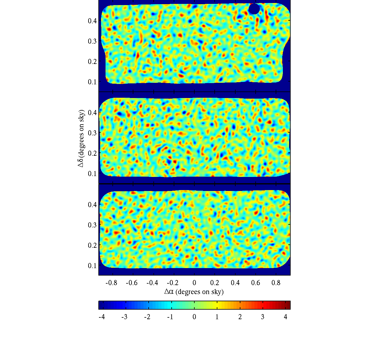
Figure 3.— Significance (snr) maps for the SZA4, DLS, and NOAO NDWFS fields after source removal and rescaling by the noise. Note the region excluded in the top map due to the limited dynamic range of the SZA. We see no dark regions of significance greater than 4.3.

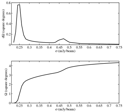
Figure 4.— Area as a function of Sensitivity for the SZA survey. In the top panel we show the differential area as function of sensitivity ( d${\rm\sigma=0.01~{}mJy/beam}$). Notice the high bump near a sensitivity of 0.25 mJy/beam that encompasses most of our survey area. The smaller bump near a coverage of 0.47 mJy/beam is a result of the shallow coverage on half of the SZA4 field. In the bottom panel we present the integrated area of the survey as a function of sensitivity.

Table 3SZA Area Coverage

Noise Value	$\sum$ Area($<$noise)
(mJy)	($\deg^{2}$)
0.22	0.000
0.23	0.041
0.24	0.287
0.25	1.043
0.26	1.807
0.27	2.179
0.28	2.365
0.29	2.476
0.30	2.568
0.35	2.892
0.40	3.116
0.45	3.354
0.50	3.823
0.55	4.013
0.60	4.120
0.65	4.207
0.70	4.278
0.75	4.336

We calculate numerically the differential survey area as a function of rms  noise on intervals of d${\rm\sigma=0.01~{}mJy/beam}$, shown in the top panel of Figure 4. Over most of the survey area, the noise lies between 0.25 and 0.3 mJy/beam. In the bottom panel we present the integral of the top panel to indicate the total survey area as a function of sensitivity; the same data are presented in tabular format in Table 3.

3.2. Cluster Detection

Once we have removed sources of emission and rescaled by the noise, we search for clusters as decrements in the mosaicked maps. We consider a detection any pixel whose amplitude is at least 5  times the rms  noise level. Note that the Fourier-space coverage of the compact array was designed to match the typical cluster profile, so that these mosaics have already been optimally filtered for cluster detection.

No clusters were identified at $>5\sigma$ significance, with the largest decrement having a significance of 4.3$\sigma$. This allows us to place an upper limit on $\sigma_{8}$.

4. Expected Number of Clusters

The number of clusters of mass $M$ that we should detect, per unit noise and redshift interval, is given by

$${{dN}\over{dM\,d\sigma\,dz}}(M,\sigma,\sigma_{8}) =$$

$$p(D|M,z,\sigma) \times {{dN}\over{dM\,d\Omega\,dz}}(M,z,\sigma_{8})\times{{d\Omega}\over{d\sigma}}(\sigma)$$ (2)

where $p(D|M,z,\sigma)$ is the completeness, the probability of detecting a cluster of mass $M$ at redshift $z$ in the presence of noise $\sigma$, ${\frac{dN}{dMd\Omega~{}dz}(M,z,\sigma_{8})}$ is the mass function, the predicted density of clusters as a function of mass, redshift, and $\sigma_{8}$, and $\frac{d\Omega}{d\sigma}(\sigma)$ is the survey area as a function of noise level.

The total number of clusters we expect to detect for a given cosmology is then given by the integral of Equation 4 over mass, redshift and map noise:

$$N(\sigma_{8})=\int{dz}\int{d\sigma}\int{{{dN}\over{dM\ d\sigma~{}dz}}(M,\sigma,\sigma_{8})\,dM.}$$ (3)

Here we assume the concordance cosmological parameters from WMAP 7-year results (Larson et al. 2010).

4.1. The Mass Function

We assume the mass function of dark matter halos derived from cosmological simulations of flat ${\rm\Lambda CDM}$ cosmology. We adopt the fitting formula of Tinker et al. (2008), and assume a redshift evolution for the over-density parameter given by the growth factor of Viana & Liddle (1996).

4.2. Completeness

As indicated in Equation 1, the fundamental SZ observable is the compton-$y$ parameter. We can relate this observable to the cluster mass either through observation or simulation, both of which are subject to significant uncertainties. SZ-effect and X-ray observations can be used to determine scaling relations between compton-$y$ and cluster mass (e.g., Bonamente et al. 2008), but these observations typically comprise a small number of massive clusters spanning a limited redshift range, and often relate quantities determined at overdensity radii not directly comparable to those sampled by a particular experiment. By contrast, simulations can be accurately compared to experimental details, but the correspondence between the SZ observable and cluster mass is highly dependent on the accuracy of the simulated gas thermodynamics (Kravtsov et al. 2005).

We use the simulation of Shaw et al. (2009) (hereafter S09) to translate between compton-$y$ and cluster mass. This simulation combines an N-body ‘lightcone’ simulation with a semi-analytic model for the cluster gas, with a significant amount of heating from feedback processes (i.e., AGN feedback, star formation). Gas parameters in S09 have also been adjusted to match X-ray observations of low-redshift clusters. We select clusters from 40 compton-$y$ maps, each 5 degrees on a side, with ${\rm M_{200}}$ masses ranging from ${\rm 2.5\times 10^{13}~{}M_{\odot}}$ to ${\rm 3.0\times 10^{15}~{}M_{\odot}}$, where ${\rm M_{200}}$ is the mass enclosed within a radius corresponding to an overdensity of 200 times the mean density of the universe; it is this mass that we refer to in all subsequent discussion.

To calculate the probability that the SZA would detect a cluster of a given mass, mock observations of the y-maps are performed in survey mode, in a multi-pointing mosaic scheme. For computational expediency, we do not simulate observations of large areas of simulated sky, but select individual clusters from the catalog and calculate what fraction of them would have been detected. Each simulated cluster is placed at the center of a small field, 0.47^∘ on a side. On this image we overlay a grid of pointings in a 2-3-2 hex pattern, reflecting the spacings in our survey. The cluster image is weighted by the primary beam (centered at each pointing), and the result is Fourier-transformed and re-sampled onto a $uv$-grid that reflects the actual coverage of the survey data. To the visibilities in each pointing we add Gaussian noise, with weights chosen such that the resulting noise in the image plane mosaic is uniform in a region within a 4′ radius of the cluster. To quantify the cluster detectability as a function of noise, we generate maps with rms noise between $0.2-0.65$ mJy/beam, in steps of $0.05$ mJy/beam.

To simulate the effect of compact source contamination, we add unresolved sources brighter than 0.05 mJy to the data according to the M10 distribution for regions further than 0′.5 from the cluster center. To account for cluster-source correlations we add sources brighter than 0.01 mJy according to the distribution from Coble et al. (2007) for regions near the cluster center. To mimic our source-extraction algorithm, we generate a 5 GHz flux for each source from the spectral index distribution of M10, and create a 5-GHz source catalog of all sources brighter than 0.35 mJy (the detection threshold for our VLA 5-GHz source catalog). Sources are extracted from the simulated maps exactly as described in §2.6, with the exception that we remove a perfect model from the simulated data rather than a fitted flux and spectral index, in the interest of computational speed. We have verified that this does not systematically bias our results by comparing the fitted flux of sources in these simulations with their original values, i.e., the presence of noise introduces a random error into the fit flux of the source, yet over the many realizations performed we recover the true flux of the source.

Once the identified sources are removed from the mock observation, we search for the peak decrement in the short-baseline mosaics, within the region of uniform noise in our mock observation (namely 4′). We identify clusters in the simulated data as described in §3.2.

To capture the inherent flux distribution for clusters of similar mass, as well as the redshift evolution of clusters, clusters were observed in nine different mass ranges ($M_{\rm min}={\rm 1.5\times 10^{14}~{}M_{\odot}}$, $\Delta M={\rm 10^{14}~{}M_{\odot}}$) and eight redshift bins ($z_{\rm min}=0.1$, $\Delta z=0.2$). The number of clusters observed in each mass range and redshift bin varied from 2 to 200; some bins contained no clusters, namely the high-mass, high-redshift bins. We further select only clusters which are not within 0.23^∘ of the edge of the simulated maps, and which are not within 4 arcminutes of clusters of greater or comparable masses. The first cut ensures we do not introduce artifacts associated with field edges, and the second ensures that our observations are of clusters whose masses are well-defined, i.e., whose simulated masses are not corrupted by the presence of secondary clusters. For each mass and redshift bin, we iterate over 200 distinct realizations of clusters, noise and compact sources.

To calculate the resulting completeness, we determine the fraction of time the clusters in a given bin were detected at significance greater than ${\rm 5\sigma}$.

4.3. Survey Mass Limit

Equipped with the survey completeness (§4.2) and the area as a function of noise (§3.1), we can calculate the area as a function of mass and redshift. As the SZ effect depends most directly on cluster mass, this can be used to calculate the redshift-dependent mass limit of our survey, which we present in Figure 5 for the S09 simulations. For each redshift bin, we present the ${\rm M_{200}}$ mass above which our survey is 50% complete. As expected, the mass limit decreases towards higher redshifts, as clusters become more compact and therefore more easily detectable by the SZA.

In Figure 5, we also present the limiting mass calculated from a different simulation, White (2003), to demonstrate the effect of gas physics in our completeness calculations. The differences between the simulations and their effect on our results are discussed in detail in §6.

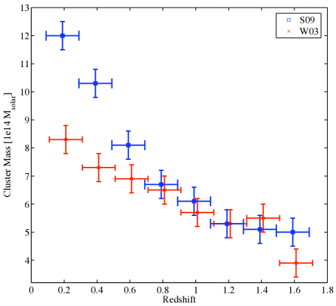
Figure 5.— The mass limit of the SZA survey calculating using the area as a function of noise, and cluster detectability from simulations of S09 (square points) and W03 (See §6). The points correspond to the ${\rm M_{200}}$ mass of a cluster which would have been detected at least 50% of the time, and are offset from each other in redshift for ease of presentation. The differences between values are a result of the W03 simulations not including AGN feedback or “pre-heating” in calculating the compton-$y$ parameter.

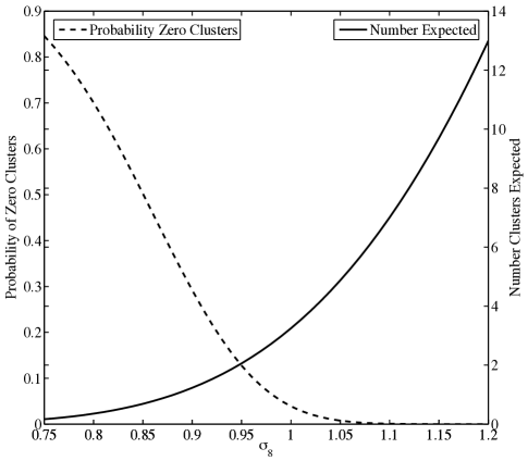
Figure 6.— Expected number of clusters (and the probability of non-detection of clusters) in the 4.4 square degree SZA survey, as a function of $\sigma_{8}$, using WMAP cosmology for all other parameters and cluster detectability from S09 simulations. The solid line represents the expected number of clusters, with the corresponding scale presented on the right axis. The dashed line is the probability of detecting zero clusters, with the corresponding scale on the left axis.

5. Constraint on $\sigma_{8}$

To calculate the value of $\sigma_{8}$ which is most consistent with the SZA survey, we address the question: what is the probability of a $\sigma_{8}$ value given the number of observed clusters, $P(\sigma_{8}|N)$? A simple invocation of Bayes’ theorem yields:

$$P(\sigma_{8}|N)\propto P(N|\sigma_{8})P(\sigma_{8})$$ (4)

where $P(N|\sigma_{8})$ is the probability of $N$ detections given a value of $\sigma_{8}$ and $P(\sigma_{8})$ is the prior on $\sigma_{8}$, which we take to be uniform.

The number of clusters detected is a Poisson process, with a well-defined distribution given by

$$P(k|\lambda)=\frac{e^{-\lambda}\lambda^{k}}{k!}$$ (5)

where $P(k|\lambda)$ is the probability that a process with expectation $\lambda$ occurs $k$ times. As we detect no cluster candidates in the SZA survey (at a significance greater than $5\sigma$), we have $k$=0, whence

$$P(\sigma_{8}|N)=e^{-N(\sigma_{8})}$$ (6)

where $N(\sigma_{8})$ is the result from Equation 3, shown pictorially in Figure 6. Note that in determining $N(\sigma_{8})$, we adopt concordance cosmological parameters from WMAP 7-year results (Larson et al. 2010), and calculate for completeness determined from the S09 simulations. Figure 6 (via Equation 6) can be used to compare the relative likelihood of different values of $\sigma_{8}$. For example, we expect a non-detection in the SZA survey $5\%$ of the time if ${\rm\sigma_{8}}=0.97$.

We integrate Equation 6 to generate the probability, given our data, that $\sigma_{8}$ exceeds a given value; the result is presented in Figure 7. We see that for the S09 simulation, $\sigma_{8}$ values of greater than 0.84 are ruled out at 95% confidence.

In calculating this limit, we have made the conventional assumption of a “non-informative” prior (i.e., uniform for ${\rm\sigma_{8}}\ >0$). While we consider this approach conservative, in that it captures what the SZA data can say about the value of $\sigma_{8}$ under a minimal set of prior assumptions, note that it will also lead to the tightest possible (for uniform priors) constraint on $\sigma_{8}$. If for example, the prior were truncated to ${\rm\sigma_{8}}\ >0.5$, our $95\%$ limit would shift to ${\rm\sigma_{8}}<0.87$. Sensitivity to the prior is typical for data sets with unequal power to discriminate among allowable hypotheses; in this case, the small area of the SZA survey can strongly rule out high values of $\sigma_{8}$, but provides little or no power to discriminate against low values of $\sigma_{8}$, to which our prior nonetheless assigns equal weight.

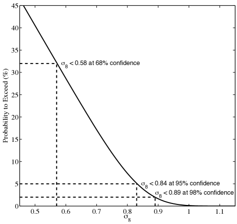
Figure 7.— Plot of the probability of that $\sigma_{8}$ exceeds a given value for completeness derived using the S09 simulations, with the 1-, 2-, and 3-$\sigma$ confidence limits presented.

6. Systematics

The conversion from cluster mass to SZ observable is potentially the largest systematic uncertainty in cosmological analyses of SZ surveys. Because constraints on $\sigma_{8}$ are determined by comparison with simulations, they are necessarily sensitive to the assumptions that underlie each simulation’s modeling of the ICM. As a rough estimate of the importance of model assumptions to our limit on $\sigma_{8}$, we repeat our analysis using the simulation of White (2003) (hereafter W03), a high-resolution N-body simulation following the semi-analytic method of Schulz & White (2003). The salient difference between the S09 and W03 simulations is that S09 incorporate AGN and supernovae feedback while W03 ignore cold gas and star formation. As a result, clusters in the W03 simulation tend to be more compact (and therefore more detectable by the SZA), with higher central SZ-decrements than equivalent clusters (by mass) in S09. This leads to a higher completeness for W03 clusters of a given mass, a lower mass limit (See Figure 5), and a stronger constraint on $\sigma_{8}$ (a 95% confidence limit that is lower by 0.04). We choose to present the limit derived from S09 in §5 not only because it is the more conservative of the two, but also because the S09 simulation represents a more realistic model of ICM physics; we nevertheless caution that significant uncertainties in the modeling of cluster gas physics remain.

In the completeness calculation described in §4.2, we model the correlation between clusters and radio sources by using the Coble et al. (2007) source distribution for the inner regions of clusters, and the M10 distribution for field sources. However the Coble et al. (2007) distribution was determined from observations of the most massive clusters, and can bias our completeness low if sources are over-represented in these objects relative to the lower-mass clusters to which the SZA is sensitive. To bracket the magnitude of this effect, we repeat the completeness calculations described in §4.2 without using the Coble et al. (2007) over-densities, i.e., using the source counts obtained only from field sources presented in M10. Neglecting the higher density of sources towards galaxy clusters increases our completeness on the order of 12%, which due to the steepness of the dependence of cluster counts on $\sigma_{8}$  would lower our limit by 0.04.

In §2.6 we mentioned that for one bright source, the limited dynamic range of the SZA introduces a hole in our coverage at the source location. If the correlation between clusters and radio sources had not properly been taken into account in calculating our completeness, this would bias our completeness low if bright sources are preferentially associated with galaxy clusters. However, we simulate both the correlation and the corresponding reduction in completeness entailed by missing clusters associated with sources that we cannot subtract; cutting such sources out of our maps therefore corresponds to a simple reduction in the survey area, and should have no effect on our limit.

Although we see no evidence of sources which are resolved by the long-baseline data, as discussed in §2.6, we fit the 12% of sources deemed to be extended at 5 GHz to a combination of the long and short-baseline data (whereas sources deemed a priori to be unresolved were fit only to the long-baseline maps). If any of these sources happened to be associated with a cluster, the cluster decrement present in the short-baseline data would reduce the fitted flux of the source, resulting in residual source flux in the map that would bias against detecting the cluster. To quantify this effect, we re-calculate the completeness with a slight modification in 12% of the realizations, namely that we do not remove the true flux of the source, but instead remove the map flux at the source location in the combination of short and long baseline maps. As the majority of sources are not associated with clusters, this test can be thought of an upper limit to any potential reduction in our completeness. Properly accounting for this effect would raise our limit on $\sigma_{8}$ by at most 0.01.

An additional source of uncertainty unrelated to our analysis methods is the clustering of large-scale structure. We know that galaxy clusters are not evenly distributed throughout space, but form preferentially along filaments. As a result, the number of clusters seen in small fields such as those observed by the SZA do not follow a Poisson distribution. In particular, since most lines of sight will sample the voids between filaments, this leads to an increased probability of detecting fewer massive halos than the Poisson average. To quantify the impact on our results, we begin with the 100 square degree W03 simulations. We select regions similar in shape, size and noise properties to each of our fields from the simulated maps, and fold in the calculated completeness to estimate the number of clusters we should detect. We do this for $>10^{4}$ realizations of each of the three SZA fields, varying the location and orientation of the field over the sky-map, to generate a distribution of expected numbers of clusters, and compare this to the Poisson prediction for the equivalent field size and input $\sigma_{8}$. The result is a 10% increase in the probability of a non-detection for an input $\sigma_{8}$ of 0.9 over the Poisson prediction, leading to an underestimate of the true $\sigma_{8}$. Accounting for this effect, assuming similar clustering over a range of $\sigma_{8}$, would raise our limit by at most 0.04.

Lastly, as described in M10, the calibration of the SZA data is tied to the modeled flux of Mars, which we estimate is accurate to $\lesssim 10\%$. A shift in the flux of Mars corresponds to a simple rescaling of the map noise, and consequently a shift in the completeness. As noted above, a change in the completeness of $\lesssim 10\%$ corresponds to a shift in our limit on $\sigma_{8}$ (in either direction) of $\lesssim 0.04$.

7. Discussion

From 2005 to 2007, the SZA performed a  6.1 square degree survey for clusters of galaxies via their SZ effect at 31 GHz. In one of the fields there is evidence for large-scale dust-correlated emission; this field was excluded from the analysis presented here. Of the remaining 4.4 square degrees of the survey suitable for cosmological analysis, we estimate that the survey is $50\%$ complete to a mass of ${\rm M_{200\overline{\rho}}\sim 6\times 10^{14}~{}M_{\odot}}$, averaged over redshift. By comparison with simulations, we place an upper limit on the value of $\sigma_{8}$ of ${\rm 0.84~{}(+0.07)}$ at 95% confidence, where the uncertainty reflects calibration and systematic uncertainties discussed in §6, excluding the error associated with the simulated cluster gas physics. Although this last uncertainty is potentially the dominant one, to properly quantify it requires a calculation of the completeness for a wide range of simulations with realistic gas models, which is beyond the scope of this paper.

Our limit on $\sigma_{8}$ is consistent with recent results from SZ surveys performed over larger areas of sky, such as with the South Pole Telescope (Vanderlinde et al. 2010), and with determinations of $\sigma_{8}$ from gravitational lensing and X-ray cluster surveys (Smith et al. 2003; Allen et al. 2003). In addition, it is consistent with determinations of $\sigma_{8}$ from CMB anisotropy measurements, namely those of WMAP (Dunkley et al. 2009), the South Pole Telescope (Lueker et al. 2010), and the Atacama Cosmology Telescope (Fowler et al. 2010). Our constraint is also in agreement with that of Sharp et al. (2010), based on CMB anisotropy measurements with the SZA itself. Although the data were collected with the same instrument, we note that both the data sets and the analyses of this paper and of Sharp et al. (2010) are completely independent.

References

- Allen et al. (2003) Allen, S. W., Schmidt, R. W., Fabian, A. C., & Ebeling, H. 2003, MNRAS, 342, 287
- Birkinshaw (1999) Birkinshaw, M. 1999, Physics Reports, 310, 97
- Bonamente et al. (2008) Bonamente, M., Joy, M., LaRoque, S. J., Carlstrom, J. E., Nagai, D., & Marrone, D. P. 2008, ApJ, 675, 106
- Carlstrom et al. (2002) Carlstrom, J. E., Holder, G. P., & Reese, E. D. 2002, ARA&A, 40, 643
- Clegg (1980) Clegg, P. E. 1980, Phys. Scr, 21, 678
- Coble et al. (2007) Coble, K., Bonamente, M., Carlstrom, J. E., Dawson, K., Hasler, N., Holzapfel, W., Joy, M., La Roque, S., Marrone, D. P., & Reese, E. D. 2007, AJ, 134, 897
- Dunkley et al. (2009) Dunkley, J., Komatsu, E., Nolta, M. R., Spergel, D. N., Larson, D., Hinshaw, G., Page, L., Bennett, C. L., Gold, B., Jarosik, N., Weiland, J. L., Halpern, M., Hill, R. S., Kogut, A., Limon, M., Meyer, S. S., Tucker, G. S., Wollack, E., & Wright, E. L. 2009, ApJS, 180, 306
- Fowler (2004) Fowler, J. W. 2004, in Society of Photo-Optical Instrumentation Engineers (SPIE) Conference Series, Vol. 5498, Society of Photo-Optical Instrumentation Engineers (SPIE) Conference Series, ed. C. M. Bradford, P. A. R. Ade, J. E. Aguirre, J. J. Bock, M. Dragovan, L. Duband, L. Earle, J. Glenn, H. Matsuhara, B. J. Naylor, H. T. Nguyen, M. Yun, & J. Zmuidzinas, 1–10
- Fowler et al. (2010) Fowler, J. W., Acquaviva, V., Ade, P. A. R., Aguirre, P., Amiri, M., Appel, J. W., Barrientos, L. F., Battistelli, E. S., Bond, J. R., Brown, B., Burger, B., Chervenak, J., Das, S., Devlin, M. J., Dicker, S. R., Doriese, W. B., Dunkley, J., Dünner, R., Essinger-Hileman, T., Fisher, R. P., Hajian, A., Halpern, M., Hasselfield, M., Hernández-Monteagudo, C., Hilton, G. C., Hilton, M., Hincks, A. D., Hlozek, R., Huffenberger, K. M., Hughes, D. H., Hughes, J. P., Infante, L., Irwin, K. D., Jimenez, R., Juin, J. B., Kaul, M., Klein, J., Kosowsky, A., Lau, J. M., Limon, M., Lin, Y., Lupton, R. H., Marriage, T. A., Marsden, D., Martocci, K., Mauskopf, P., Menanteau, F., Moodley, K., Moseley, H., Netterfield, C. B., Niemack, M. D., Nolta, M. R., Page, L. A., Parker, L., Partridge, B., Quintana, H., Reid, B., Sehgal, N., Sievers, J., Spergel, D. N., Staggs, S. T., Swetz, D. S., Switzer, E. R., Thornton, R., Trac, H., Tucker, C., Verde, L., Warne, R., Wilson, G., Wollack, E., & Zhao, Y. 2010, ApJ, 722, 1148
- Jannuzi & Dey (1999) Jannuzi, B. T. & Dey, A. 1999, in Astronomical Society of the Pacific Conference Series, Vol. 191, Photometric Redshifts and the Detection of High Redshift Galaxies, ed. R. Weymann, L. Storrie-Lombardi, M. Sawicki, & R. Brunner, 111–+
- Kravtsov et al. (2005) Kravtsov, A. V., Nagai, D., & Vikhlinin, A. A. 2005, ApJ, 625, 588
- Larson et al. (2010) Larson, D., Dunkley, J., Hinshaw, G., Komatsu, E., Nolta, M. R., Bennett, C. L., Gold, B., Halpern, M., Hill, R. S., Jarosik, N., Kogut, A., Limon, M., Meyer, S. S., Odegard, N., Page, L., Smith, K. M., Spergel, D. N., Tucker, G. S., Weiland, J. L., Wollack, E., & Wright, E. L. 2010, ArXiv e-prints
- Lueker et al. (2010) Lueker, M., Reichardt, C. L., Schaffer, K. K., Zahn, O., Ade, P. A. R., Aird, K. A., Benson, B. A., Bleem, L. E., Carlstrom, J. E., Chang, C. L., Cho, H., Crawford, T. M., Crites, A. T., de Haan, T., Dobbs, M. A., George, E. M., Hall, N. R., Halverson, N. W., Holder, G. P., Holzapfel, W. L., Hrubes, J. D., Joy, M., Keisler, R., Knox, L., Lee, A. T., Leitch, E. M., McMahon, J. J., Mehl, J., Meyer, S. S., Mohr, J. J., Montroy, T. E., Padin, S., Plagge, T., Pryke, C., Ruhl, J. E., Shaw, L., Shirokoff, E., Spieler, H. G., Stalder, B., Staniszewski, Z., Stark, A. A., Vanderlinde, K., Vieira, J. D., & Williamson, R. 2010, ApJ, 719, 1045
- Muchovej et al. (2010) Muchovej, S., Leitch, E., Carlstrom, J. E., Culverhouse, T., Greer, C., Hawkins, D., Hennessy, R., Joy, M., Lamb, J., Loh, M., Marrone, D. P., Miller, A., Mroczkowski, T., Pryke, C., Sharp, M., & Woody, D. 2010, ApJ, 716, 521
- Muchovej et al. (2007) Muchovej, S., Mroczkowski, T., Carlstrom, J. E., Cartwright, J., Greer, C., Hennessy, R., Loh, M., Pryke, C., Reddall, B., Runyan, M., Sharp, M., Hawkins, D., Lamb, J. W., Woody, D., Joy, M., Leitch, E. M., & Miller, A. D. 2007, ApJ, 663, 708
- Pospieszalski et al. (1995) Pospieszalski, M. W., Lakatosh, W. J., Nguyen, L. D., Lui, M., Liu, T., Le, M., Thompson, M. A., & Delaney, M. J. 1995, IEEE MTT-S Int. Microwave Symp., 1121
- Rudy (1987) Rudy, D. J. 1987, PhD thesis, California Institute of Technology, Pasadena.
- Ruhl et al. (2004) Ruhl, J., Ade, P. A. R., Carlstrom, J. E., Cho, H.-M., Crawford, T., Dobbs, M., Greer, C. H., Halverson, N. W., Holzapfel, W. L., Lanting, T. M., Lee, A. T., Leitch, E. M., Leong, J., Lu, W., Lueker, M., Mehl, J., Meyer, S. S., Mohr, J. J., Padin, S., Plagge, T., Pryke, C., Runyan, M. C., Schwan, D., Sharp, M. K., Spieler, H., Staniszewski, Z., & Stark, A. A. 2004, in Astronomical Structures and Mechanisms Technology. Edited by Antebi, Joseph; Lemke, Dietrich. Proceedings of the SPIE, Volume 5498, pp. 11-29 (2004)., ed. J. Zmuidzinas, W. S. Holland, & S. Withington
- Schulz & White (2003) Schulz, A. E. & White, M. 2003, ApJ, 586, 723
- Sharp et al. (2010) Sharp, M. K., Marrone, D. P., Carlstrom, J. E., Culverhouse, T., Greer, C., Hawkins, D., Hennessy, R., Joy, M., Lamb, J., Leitch, E., Loh, M., Miller, A. D., Mroczkowski, T., Muchovej, S., Pryke, C., & Woody, D. 2010, ApJ, 713, 82
- Shaw et al. (2009) Shaw, L. D., Zahn, O., Holder, G. P., & Doré, O. 2009, ApJ, 702, 368
- Smith et al. (2003) Smith, G. P., Edge, A. C., Eke, V. R., Nichol, R. C., Smail, I., & Kneib, J.-P. 2003, ApJ, 590, L79
- Sunyaev & Zel’dovich (1972) Sunyaev, R. A. & Zel’dovich, Y. B. 1972, Comments Astrophys. Space Phys., 4, 173
- Sunyaev & Zel’dovich (1980) —. 1980, ARA&A, 18, 537
- Tinker et al. (2008) Tinker, J., Kravtsov, A. V., Klypin, A., Abazajian, K., Warren, M., Yepes, G., Gottlöber, S., & Holz, D. E. 2008, ApJ, 688, 709
- Vanderlinde et al. (2010) Vanderlinde, K., Crawford, T. M., de Haan, T., Dudley, J. P., Shaw, L., Ade, P. A. R., Aird, K. A., Benson, B. A., Bleem, L. E., Brodwin, M., Carlstrom, J. E., Chang, C. L., Crites, A. T., Desai, S., Dobbs, M. A., Foley, R. J., George, E. M., Gladders, M. D., Hall, N. R., Halverson, N. W., High, F. W., Holder, G. P., Holzapfel, W. L., Hrubes, J. D., Joy, M., Keisler, R., Knox, L., Lee, A. T., Leitch, E. M., Loehr, A., Lueker, M., Marrone, D. P., McMahon, J. J., Mehl, J., Meyer, S. S., Mohr, J. J., Montroy, T. E., Ngeow, C., Padin, S., Plagge, T., Pryke, C., Reichardt, C. L., Rest, A., Ruel, J., Ruhl, J. E., Schaffer, K. K., Shirokoff, E., Song, J., Spieler, H. G., Stalder, B., Staniszewski, Z., Stark, A. A., Stubbs, C. W., van Engelen, A., Vieira, J. D., Williamson, R., Yang, Y., Zahn, O., & Zenteno, A. 2010, ApJ, 722, 1180
- Viana & Liddle (1996) Viana, P. T. P. & Liddle, A. R. 1996, MNRAS, 281, 323
- White (2003) White, M. 2003, ApJ, 597, 650
- Wittman et al. (2002) Wittman, D. M., Tyson, J. A., Dell’Antonio, I. P., Becker, A., Margoniner, V., Cohen, J. G., Norman, D., Loomba, D., Squires, G., Wilson, G., Stubbs, C. W., Hennawi, J., Spergel, D. N., Boeshaar, P., Clocchiatti, A., Hamuy, M., Bernstein, G., Gonzalez, A., Guhathakurta, P., Hu, W., Seljak, U., & Zaritsky, D. 2002, in Society of Photo-Optical Instrumentation Engineers (SPIE) Conference Series, Vol. 4836, Society of Photo-Optical Instrumentation Engineers (SPIE) Conference Series, ed. J. A. Tyson & S. Wolff, 73–82