Velocity Structure Diagnostics of Simulated Galaxy Clusters

Abstract

Gas motions in the hot intracluster medium of galaxy clusters have an important effect on the mass determination of the clusters through X–ray observations. The corresponding dynamical pressure has to be accounted for in addition to the hydrostatic pressure support to achieve a precise mass measurement. An analysis of the velocity structure of the ICM for simulated cluster–size haloes, especially focusing on rotational patterns, has been performed, demonstrating them to be an intermittent phenomenon, strongly related to the internal dynamics of substructures. We find that the expected build–up of rotation due to mass assembly gets easily destroyed by passages of gas–rich substructures close to the central region. Though, if a typical rotation pattern is established, the corresponding mass contribution is estimated to be up to $\sim 17\%$ of the total mass in the innermost region, and one has to account for it. Extending the analysis to a larger sample of simulated haloes we statistically observe that (i) the distribution of the rotational component of the gas velocity in the innermost region has typical values of $\sim 200-300\rm{km/s};$ (ii) except for few outliers, there is no monotonic increase of the rotational velocity with decreasing redshift, as we would expect from approaching a relaxed configuration. Therefore, the hypothesis that the build–up of rotation is strongly influenced by internal dynamics is confirmed, and minor events like gas–rich substructures passing close to the equatorial plane can easily destroy any ordered rotational pattern.

1 Introduction

Within the hierarchical structure–formation scenario, galaxy clusters are key targets that allow us to study both the dynamics on the gravity–dominated scale and the complexity of astrophysical processes dominating on the small scale. In such studies their mass is one of the most crucial quantities to be evaluated, and the bulk properties measured from X–ray observations still provide the best way to estimate the mass, primarily on the assumption of hydrostatic equilibrium Sarazin (1988). Mass estimates rely then on the assumptions made about the cluster dynamical state, since the Hydrostatic Equilibrium Hypothesis (HEH) implies that only the thermal pressure of the hot ICM is taken into account Rasia, Tormen & Moscardini (2004). Lately, it has been claimed in particular that non–thermal motions, as rotation, could play a significant role in supporting the ICM in the innermost region (e.g. Lau, Kravtsov & Nagai, 2009; Fang, Humphrey & Buote, 2009) biasing the mass measurements based on the HEH. The analysis of simulated cluster–like objects provides a promising approach to get a better understanding of the intrinsic structure of galaxy clusters and the role of gas dynamics, which can be eventually compared to X–ray observations. Because of the improvement of numerical simulations, the possibility to study in detail the physics of clusters has enormously increased (see Borgani & Kravtsov, 2009, for a recent comprehensive review) and future satellites dedicated to high–precision X–ray spectroscopy, such as ASTRO–H and IXO, will allow to detect these ordered motions of the ICM. With this perspective, we perform a preliminary study on the ICM structure for some clusters extracted from a large cosmological hydrodynamical simulation, investigating in particular the presence of rotational motion in the ICM velocity field.
The paper is organized as follows. We describe the numerical simulations from which the samples of cluster–like haloes have been selected in Section 2. In Section 3 we consider a first set of simulated clusters and present results on build–up of rotation in the halo core for single cases of study (Section 3.1 and Section 3.2), while results about the contribution to the mass estimations are given in Section 4. A second sample of clusters is then statistically investigated in Section 5. We discuss our results and conclude in Section 6.
Appendix A is devoted to comment on the effects of artificial viscosity, while in Appendix B we briefely comment on the ellipticity profiles of the simulated clusters.

2 Numerical Simulations

We consider two sets of cluster–like haloes selected from two different parent cosmological boxes. In both cases the cosmological simulations were performed with the TreePM/SPH code GADGET–2 Springel, White & Hernquist (2001); Springel (2005), assuming a slightly different cosmological model (a standard $\Lambda$CDM model and a WMAP3 cosmology, respectively) but including the same physical processes governing the gas component Springel & Hernquist (2003), i.e. radiative cooling, star formation, and supernova feedback (csf simulation, see Dolag et al. (2009) and references therein for a more detailed overview on different runs of the parent hydrodynamical simulations we refer to in our work). Additionally, we refer to simulations of the same objects without including radiative processes as ovisc.
Set 1. The first data set considered consists of 9 cluster–size haloes, re–simulated with higher resolution using the “zoomed initial condition”(ZIC) technique Tormen, Bouchet & White (1997). The clusters have been originally extracted from a large–size cosmological simulation of a $\Lambda$CDM universe with $\Omega_{0}=0.3$, $h=0.7$, $\sigma_{8}=0.9$ and $\Omega_{b}=0.039$, within a box of $479h^{-1}\rm{Mpc}$ a side. The final mass–resolution of these simulations is $m_{DM}=1.13\times 10^{9}h^{-1}\rm{M_{\odot}}$ and $m_{gas}=1.69\times 10^{8}h^{-1}\rm{M_{\odot}},$ for the DM and gas particles, respectively. The spatial resolution for Set 1 reaches $5h^{-1}\rm{kpc}$ in the central parts and for the most massive clusters we typically resolve up to 1000 self–bound sub–structures within $R_{vir}$ (as shown in Dolag et al., 2009). The main haloes have masses larger than $\sim 1.1\times 10^{14}h^{-1}\rm{M_{\odot}}$ and they have all been selected in a way that they are quite well–behaved spherically–shaped objects at present epoch, although a fair range from isolated and potentially relaxed objects to more disturbed systems embedded within larger structures is available. Having a reasonable dense sample within the time domain (e.g. 50 outputs between $z=1$ and today) and high resolution, we can study how common and significant the rotational support of the ICM is. In particular we focus on the detailed evolution of such rotational motions.
Set 2. In the second data set we analyzed a volume limited sample of cluster–size haloes, where we computed the distribution of the ICM rotational velocity and compared their distribution at different redshift. This second set of clusters has been extracted from a large size cosmological simulation with a box–size of $300h^{-1}\rm{Mpc},$ simulated with $2\times 768^{3}$ particles, assuming the 3–year WMAP values for the cosmological parameters Spergel et al. (2007), i.e. $\Omega_{0}=0.268$, $\Omega_{b}=0.044$, $\sigma_{8}=0.776$ and $h=0.704$. The final mass–resolution for this second set of simulations is $m_{DM}=3.71\times 10^{9}h^{-1}\rm{M_{\odot}}$ and $m_{gas}=7.28\times 10^{8}h^{-1}\rm{M_{\odot}}$. Given the larger sample, a fair investigation of the amount of rotational support within the ICM from a statistical point of view is then possible.
The two sets of simulations analyzed were performed with a different value of $\sigma_{8},$ meaning that differences in the merging histories can be introduced. Nevertheless, we stress that the purpose of the second set is only to enlarge the statistics on the build–up of rotational motions in simulated galaxy clusters, and not a direct comparison of single objects to the objects of Set 1. Therefore, we are confident that our conclusions do not depend on these differences in the parameters of the two simulations.

3 VELOCITY STRUCTURE OF THE ICM

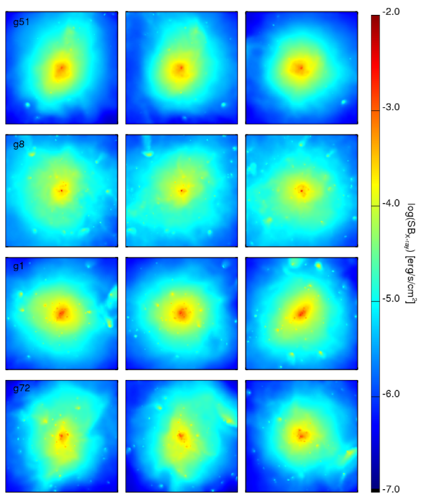
Figure 1: X–ray surface brightness maps along the three projection axis for the four most massive cluster–like haloes in Set 1 (from top to bottom: g51, g8, g1, g72). Each map is $2\rm{Mpc}$–side, enclosing therefore the region of about $\sim R_{500}$.

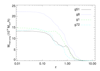
Figure 2: Main halo mass accretion history for the four most massive clusters in Set 1: g51 (solid, black line), g8 (dotted, blue), g1 (dashed, green), and g72 (dot–dashed, light–blue). The mass of the main halo is plotted in units of $10^{14}h^{-1}\rm{M_{\odot}}$ as function of redshift.

In the first place, we have been investigating the velocity structure of the ICM for all the main haloes of the Set 1, looking for evidence of rotational patterns in the most central regions of the simulated clusters, especially for the most massive haloes.
Although a variety of objects is offered (ranging from more complex structures sitting in a denser environment to quite isolated haloes), all the cluster-like haloes have been originally selected to be fairly regularly shaped. For this aspect, the whole Set 1 is biased towards quite relaxed clusters and we would expect to find a more significant amount of rotation than on average. Among the four most massive systems, for which Fig. 1 gives the X–ray surface brightness maps in the three projected directions, we identify as the most relaxed clusters g51 and g8, while g1 and g72 are disturbed systems still suffering at the present epoch from recent major mergers

An indication of this differences is clearly shown in Fig. 2, where we plot the mass accretion history for the main progenitor of each cluster as function of redshift. The curves referring to g51 and g8 (solid black line and dotted blue line, respectively) show a smoother mass assembly (at late times, i.e. $z\lesssim 0.3$) if compared with those for g1 and g72 (dashed green line and dot–dashed light–blue line, respectively), whose curves show bumps related to major merging events down to very low redshift. In addition, a visual inspection of the X–ray surface brightness maps presented in Fig. 1 definitely suggests g51 to be the less sub-structured halo.
In this perspective, we address g51 as the best case of study to explore the build–up of rotational motions in the cluster central region as a consequence of the cooling of the core. Among the other clusters also g1 shows interesting features in its velocity field that are worth to be investigated in more detail and compared to the case of g51 to better characterize the occurrence of ordered rotational motions in the intracluster gas (see Appendix B for a comment on the isophote ellipticities of g51 and g1 among the four most massive haloes from Set 1 and how the gas shapes relate to intrinsic rotational gas motions).

3.1 Rotational patterns in the ICM

The two cases analyzed in detail (the isolated regular cluster, g51, and the disturbed massive halo g1) are particularly interesting for our purpose, since their velocity structure at redshift $z=0$ shows two opposite pictures, namely strong rotational patterns for g1 and almost no gas rotation for g51.
In the classic cooling flow model, gas rotation is expected near the center of the flow because of mass and angular momentum conservation (e.g. Mathews & Brighenti, 2003). Though, the rate of cooling gas predicted by the classical paradigm of cooling flows is rarely observed in real clusters, implying that feedback processes must play a role in preventing cooling McNamara & Nulsen (2007). In contrast, in simulations, the strong cooling in the central region of the simulated cluster–like haloes suggests that relaxed objects should build up significant rotational motion in the innermost region where gas is infalling and contracting under the conservation of angular momentum. As reported in the literature (e.g. Fang, Humphrey & Buote, 2009) this effect is expected to be particularly evident in simulated clusters that can be identified as relaxed objects. Therefore it is interesting to point out that, in our sample, not even in the object with the smoothest accretion history and less substructured morphology significant rotational patterns establish in the ICM velocity structure as a consequence of collapse.
Dealing with hydrodynamical simulations though, the build–up of rotation in the central region of clusters can be also enhanced by an excess of gas cooling that has been found to overproduce the observed cosmic abundance of stellar material (e.g Katz & White, 1993; Balogh et al., 2001) in absence of very strong, not yet fully understood feedback processes. In our simulations, the implementation of a multi–phase model for star formation (e.g. Katz, Weinberg & Hernquist, 1996; Springel & Hernquist, 2003) and the treatment of the thermal feedback process, including also galactic winds associated to star formation, is able to partially reduce the over–cooling problem Borgani et al. (2006). This fact plausibly contributes to prevent significant rotation.
In order to study in detail the rotational component of the ICM velocity for a halo, we first define a “best equatorial plane”on which we can calculate the tangential component of the velocity, $v_{tan}.$ This plane is taken to be perpendicular to the direction of the mean gas angular momentum, j, calculated averaging over the gas particles within the region where we want to investigate the rotational motion within the ICM, i.e. $<0.1R_{500}$ (here, the overdensity of $500$ is defined with respect to the critical density of the Universe). This definition of the “best equatorial plane”allows us to emphasize and characterize the rotation of the gas in an objective way for all clusters, whenever it appears.
To perform our analysis, we rotate the halo such that the new $z$–axis is aligned with the direction of j and the new $xy$ plane easily defines the best equatorial plane. After subtracting an average bulk velocity for the gas component within the region corresponding to $R_{500}$, we compute the tangential component of the velocity on this plane. We consider a $40h^{-1}\rm{kpc}$ slice of the simulation box containing this plane for all the calculations hereafter.

3.2 A case study: g51 vs. g1

Figure 3: Rotational velocity as function of the radius out to $R_{500}$ for a relaxed cluster (g51, left panel) and for a highly disturbed system (g1, right panel), at $z=0$. The tangential component of the ICM velocity is calculated on the best equatorial plane, i.e. the plane perpendicular to the direction of the mean gas angular momentum in the region within $0.1R_{500}$. Two runs are compared: the csf simulation (solid line), including radiative cooling, star formation and supernova feedback, and the ovisc simulation (dashed line), in which all these physical processes are omitted and only a treatment for artificial viscosity is considered.

As a case study, we particularly focus on g51, an isolated massive cluster with gravitational mass of $M_{200m}=1.34\times 10^{15}h^{-1}\rm{M_{\odot}}$ and a size of $R_{200m}=2.28h^{-1}\rm{Mpc}$ at $z=0$, and we compare it with the other extreme case mentioned, g1, which is instead a strongly disturbed system with $M_{200m}=1.49\times 10^{15}h^{-1}\rm{M_{\odot}}$ and $R_{200m}=2.36h^{-1}\rm{Mpc}.$ Here, $R_{200m}$ is defined as the radius enclosing the region with density equal to $200$ times the mean density of the Universe, and $M_{200m}$ is the mass within $R_{200m}.$ $M_{200m}$ has been used throughout our study as reference quantity to select haloes, but we always carry out our calculations by referring to $R_{500}$ and $M_{500},$ where the overdensity of $500$ is instead defined with respect to the critical density of Universe, motivated by a possible comparison to real X–ray observations. In the case of g51 and g1, we have $R_{500}=1.09,1.20h^{-1}\rm{Mpc}$ and $M_{500}=7.46\times 10^{14},9.98\times 10^{14}h^{-1}\rm{M_{\odot}}$ respectively, at $z=0.$
From the considerations made in Section 3 about its shape and accretion history, g51 is likely to be, in a global sense, the most relaxed object in the sample. In spite of this, at $z=0$ the velocity structure of the ICM in the innermost region is far from showing a clear rotational pattern as expected from a nearly homogeneous collapse process. However it shows some rotational pattern at intermediate redshift.
In Fig. 3 we plot the rotation velocity profile, $v_{tan}(r),$ for the two interesting cases (at $z=0$) out to $R_{500}.$ As explained in the previous Section, $v_{tan}$ is the tangential component of the ICM velocity, calculated in the best equatorial plane. In order to compute the radial profile displayed in Fig. 3, we make use of radial bins in the plane to calculate the mass–weighted average value of $v_{tan}$ of the gas particles at each $r.$ We have chosen $14h^{-1}\rm{kpc},$ as optimal bin width on the base of both resolution and statistical motivation.
The radial profiles for the rotational component of the gas velocity reflect the presence of a non–negligible rotational pattern in the ICM of the disturbed system, while no significant rotation is built up in the relaxed one. The profile of g51 (left panel in the Figure, solid curve) shows relatively low values at small radii, and increases significantly only at radii larger than $\sim 0.3R_{500}$, where the rotational component of the velocity is likely to be dominated by some bulk rotational motions, plausibly related to a subhalo orbiting in the main halo close to $R_{500}$. The value of $v_{tan}$ decreases instead with increasing $r$ for g1 (right panel in the Figure, solid curve), where the rotational velocity reaches almost $1000\rm{km/s}$ in the innermost region. Also, it is interesting to compare with the rotational velocity profile for two counterpart haloes, simulated without including star formation and cooling (dashed curves). In such simulation, referred to as ovisc simulation (see Dolag et al., 2009, as an overview) the overcooling problem is completely avoided because no stars are formed at all, and no significant rotation is expected to build up in the center of the cluster–like haloes. Let us note that for g51, the curves referring to the two simulations have a significantly similar trend, while for g1 the csf simulation (solid curve) and the non–radiative one diverge towards the center, increasing in the former and decreasing in the latter. While major events occurring close to $z=0$ in the merging history of g1 could explain the high values found for $v_{tan}$ in the innermost region, no major mergers happen to characterize the history of g51 at late time. Therefore a further zoom onto g51 is required in order to understand the details of the processes that lead to the build–up or to the disruption of gas rotation in the halo core.

Rotational velocity evolution. The possibility to track back the history of the cluster–size haloes given by simulated data, allows us to follow the redshift evolution of the rotational component of the ICM velocity in the innermost region of g51, taken to be $0.1R_{500}$. Up to $z=2$, a mass–averaged value of the tangential component of the ICM velocity has been calculated in the best equatorial plane, so that rotation can be emphasized best whenever there is one. At each redshift, the orientation of the best equatorial plane has been adjusted to be perpendicular to the direction of the mean gas angular momentum, as previously defined.
While in the literature we find an inspiring work (e.g. Fang, Humphrey & Buote, 2009) where values for the rotational velocity in the central region of a relaxed cluster–like halo rise above $1000\rm{km/s}$, in our study this never happens and values generally increase up to $650\rm{km/s}$ as a maximum, except for high peaks probably related to major merging events. These differences are likely to be related to the different amount of baryon cooling that characterizes the simulations analyzed in the work by Fang, Humphrey & Buote (2009) (extensively described in Kravtsov, Nagai & Vikhlinin, 2005; Kravtsov, Vikhlinin & Nagai, 2006; Nagai, Vikhlinin & Kravtsov, 2007) with respect to those discussed here. The stellar fraction $f_{*}(<r)=M_{*}(<r)/M(<r)$ in the central part of our Set 1 clusters (i.e. $<R_{500}$) is estimated to be smaller than in Fang, Humphrey & Buote (2009) simulations, by about a factor of $\sim 1.5$. Though, it is definitely higher than expected from observations of real clusters (e.g. Lin, Mohr & Stanford, 2003). The implementation of cooling in GADGET–2 reduces the overcooling problem, naturally preventing strong rotation to get established.
In Fig. 4 we plot the variation of $v_{tan}$ with redshift, calculated in the innermost region of g51. The peak shown around redshift $\sim 1.5$ is likely to be driven by the last major merger occurring to g51, and is not related to a quiescent build–up of mass and therefore of rotation. Instead, within the redshift range $\sim 1.5-0.5$, a general, although not smooth, increasing trend of $v_{tan}$ can be seen in the plot, which is likely to be explained as the result of the collapsing process under angular momentum conservation, although it is difficult to show it quantitatively. At lower redshift, it is worth to point out an interesting feature, that is the sudden drop of $v_{tan}$, steeply decreasing twice at $z\sim 0$ and $\sim 0.3$. The breaks in this expected general trend are not directly related to any major event, and a deeper investigation of the ICM internal dynamics has then been performed in order to understand the possible origin of this unexpected behavior.

Figure 4: Evolution with redshift of the tangential component of the ICM velocity in the innermost region ($<0.1R_{500}$) of g51.

ICM velocity maps. The panels in Fig. 5 show the two–dimensional velocity field in the best equatorial plane in the central slices of g51. Each velocity vector has a length proportional to the absolute value of the velocity in that point of the plane. The dashed circles mark the innermost region enclosed within $0.1R_{500}$ (smaller circle) and $R_{500}$ (larger circle).
The velocity maps catch one of the two major decreases in the curve of $v_{tan}$, in particular the one at roughly $z\sim 0.3$, which is the first significant break in the increasing trend shown up to redshift $\sim 0.5.$ Clearly, one can see the passage of a gas–rich subhalo (thicker circle) through the best equatorial plane, onto which the gas velocity field has been projected in the Figure. The subhalo is the only gas-rich subhalo approaching the central region of the simulated cluster.
The two panels in Fig. 5 refer to redshift $z\sim 0.314$ (top) and $z\sim 0.297$ (bottom), and show the best moment right before and after the first passage of the substructure through the equatorial plane. The steep decrease of $v_{tan}$ does not start at this moment nor does it reach the lowest value, but these two redshift snapshots have been judged to best show a plausible explanation of the suppression of rotation while it is happening. In fact, from the velocity fields we notice that the gas shows a rotational motion with velocities of $\sim 380\rm{km/s}$ in the innermost region, close to the smaller dashed circle, while the subhalo is approaching (upper panel). This rotational pattern is evidently disturbed in the lower panel, where the subhalo has already passed through the plane, its gas particles get probably stripped by the main halo gas and contribute to decrease the velocity values to $\sim 275\rm{km/s}.$
Let us stress that there are several DM–only substructures permanently moving within the cluster and close to the innermost region, but they do not disturb the build–up of rotation as gas–rich subhaloes do.
The decrease of $v_{tan}$ at redshift $\sim 0$ shows an analogous behavior.

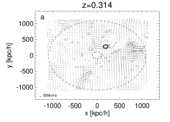
Figure 5: Gas velocity fields at $z\sim 0.314$ (upper panel) and $z\sim 0.298$ (lower panel) projected onto the plane perpendicular to the direction of the gas mean angular momentum in the innermost region. The smaller and larger dashed circles mark respectively the regions of $0.1R_{500}$ and $R_{500}$, while the grey ones are DM–only subhaloes and the black circle is the gas–rich halo passing through the equatorial plane. The coordinates in the graphs are in comoving units.

4 ROTATIONAL CONTRIBUTION TO TOTAL MASS

Figure 6: Mass profiles of the relaxed cluster g51 (upper left panel) and of the disturbed system g1 (upper right panel), at $z=0$. Top: in each panel, the radial profiles of the true mass, $M_{true}$ (solid line), and of the component estimated from the gas rotation, $M_{rot}$ (dotted line), out to $R_{500}$ are shown. Bottom: ratio of the two mass terms $M_{rot}/M_{true}$ as function of radius for g51 (lower left panel) and g1(lower right panel).

In this section we compare the contribution coming from rotational motions that should be considered in the estimation of total mass with the total mass calculated for the simulated clusters. Formally, the total cluster mass $M$ enclosed within a closed surface S is given by Gauss’s Law

$$M=\frac{1}{4\pi G}\int\nabla\Phi\cdot d^{2}\textbf{S},$$ (1)

where $\Phi$ is the cluster gravitational potential and $G$ is the gravitational constant. Under the assumptions that the ICM is a steady–state, inviscid, collisional fluid, we can replace the term $\nabla\Phi$ with the terms involving gas pressure and velocity using Euler’s equation as follows:

$$M=\frac{1}{4\pi G}\int\left[-\frac{1}{\rho_{g}}\nabla P_{g}-(\textbf{v}\cdot\nabla)\textbf{v}\right]\cdot d^{2}\textbf{S},$$ (2)

where $\rho_{g}$ and $P_{g}$ are the gas density and pressure respectively. While the pressure term within the integral represents the contribution of the gas random motions, both thermal and turbulent, the velocity term includes the ordered motions in the ICM, i.e. rotational and streaming motions. For the purpose of our work, we are mainly interested in the contribution to the pressure support given by the rotational motions of the hot intracluster gas, and we therefore separate the velocity term in Eq. 2 into

$$M_{rot}=\frac{1}{4\pi G}\int\left(\frac{v_{\theta}^{2}+v_{\phi}^{2}}{r}\right)d^{2}S$$ (3)

and

$$M_{str}=-\frac{1}{4\pi G}\int\left(v_{r}\frac{\partial v_{r}}{\partial r}+\frac{v_{\theta}}{r}\frac{\partial v_{r}}{\partial\theta}+\frac{v_{\phi}}{r\sin\theta}\frac{\partial v_{r}}{\partial\phi}\right)d^{2}S,$$ (4)

by evaluating $(\textbf{v}\cdot\nabla)\textbf{v}$ in spherical coordinates Binney & Tremaine (2008); Fang, Humphrey & Buote (2009). In particular, the term due to streaming motion, $M_{str},$ is likely to be less relevant than $M_{rot},$ especially for relaxed clusters. Therefore we explicitly calculate the rotation term for our clusters g51 and g1 at several redshifts. In our analysis we compare this term with the total “true”mass of gas and dark matter for the cluster, $M_{true},$ computed directly by summing up all the particle masses.
In Fig. 6 we show the radial profiles of both $M_{rot}$ and $M_{true},$ and their ratio, for g51 (left panel) and g1 (right panel) at $z=0.$ In order to evaluate Eq. 3 we consider the full three–dimensional structure of the velocity field without any assumption of spherical symmetry, as stated in Gauss’s theorem, so that our calculation is completely independent of the cluster geometry. In our approximation of the integral that appears in Eq. 3, the closed surface S has been replaced with a spherical shell at each radial bin, and we sum over the single particle contributions in the shell instead of dividing the surface in cells. Specifically, at each radial bin we associate an effective area to each gas particle in the shell and compute the integrand term considering the velocity $(v_{\theta}^{2}+v_{\phi}^{2})$ of the particle. We make use of a radial binning up to $R_{500},$ each bin of $14h^{-1}\rm{kpc},$ consistent with the profiles of $v_{tan}(r)$ discussed in Section 3.2.
The profiles shown in Fig. 6 have similar trends for both g51 and g1, but one can clearly notice that the more significant rotational pattern found in the innermost region of the disturbed cluster g1 with respect to g51 is reflected here in a more significant contribution to the total mass of $M_{rot}.$ In general, the rotation appears to be more important in the innermost regions than in the cluster outskirts. Indeed, out to $R_{500}$ the rotational component of the total mass accounts for $\sim 2\%$ of the true mass, $M_{true},$ in g51 and slightly more in the case of g1 ($4\%$). In contrast, $M_{rot}$ plays a more significant role at radii $<0.1R_{500},$ where its contribution can be up to $9-17\%$ of $M_{true},$ the highest value reached in the core region of g1. Although we consider purely rotational motions, other non–thermal motions should be accounted for as well and we can conclude that, if rotation establishes, it can significantly contribute to the total pressure support to the cluster weight.

5 EXTENDING THE STATISTICS TO A LARGER SIMULATED SAMPLE

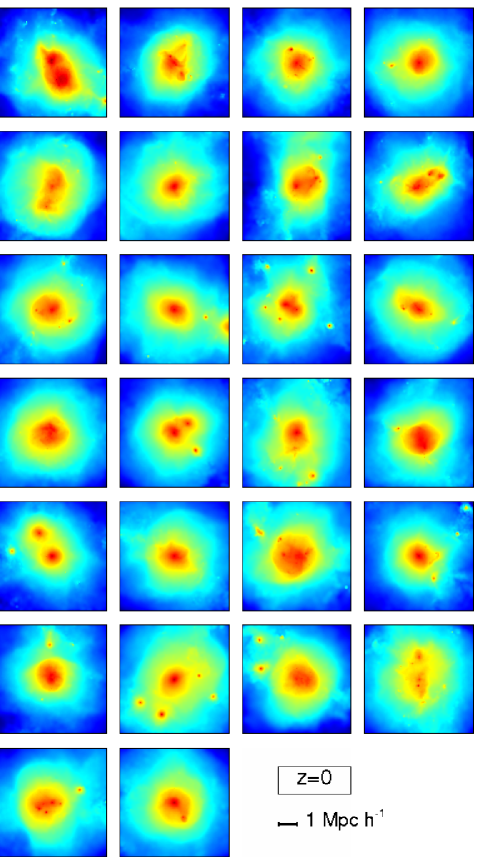
Figure 7: Visualization of the gas SB, in arbitrary units, for the 26 cluster–size haloes selected at $z=0$ from the Set 2.

In order to gain a more reliable overview of the phenomenon of the appearance of rotational patterns in the innermost regions of cluster–like haloes, our analysis has also been performed for Set 2, a larger sample of simulated objects spanning a range of $M_{200m}$ from $\sim 5\times 10^{14}h^{-1}\rm{M_{\odot}}$ to $\sim 2.2\times 10^{15}h^{-1}\rm{M_{\odot}}.$
The selection of the sample has been carried out such that we isolate all the haloes in the cosmological box with virial mass above a mass threshold, chosen to keep a statistically reliable number of objects throughout the redshift range explored. At $z=0,$ we selected 26 haloes with $M_{200m}>5\times 10^{14}h^{-1}\rm{M_{\odot}},$ for which a visual representation is given in Fig. 7. At higher redshift, the mass threshold is lower in order to have a fair sample to investigate statistically. We calculate the distribution of the rotational velocity on the best equatorial plane in the innermost region (i.e. $<0.1R_{500}$) of each selected halo, sampling the redshift range $[0,0.5]$.

5.1 Distribution of rotational velocities at various redshifts

In Fig. 8 we show the distribution of $v_{tan}$, calculated $<0.1R_{500}$ in the same way as for g51, for the sample of cluster–like haloes belonging to the Set 2. The histograms show how significant rotation is over the range of masses and redshits, confirming the intermittent nature of the phenomenon. Starting form the upper–left panel to the bottom–right one, redshift increases from $0$ to $\sim 0.5$ and the sample consists of a number of objects varying between 26 and 44. The mass threshold chosen, $M_{th},$ is $5\times 10^{14},4\times 10^{14},3\times 10^{14},2\times 10^{14}h^{-1}\rm{M_{\odot}}$ for the four redshift values considered ($z=0,0.1,0.3,0.5$, respectively). We notice that in general the velocity distributions are mainly centered around values of $200-300\rm{km/s},$ with a mild, though not substantial, shift towards higher values for intermediate redshift. The shaded histograms on top of the ones plotted for redshifts $z=0.1,0.3,0.5$ refer to subsamples of haloes with $M_{200m}>5\times 10^{14}h^{-1}\rm{M_{\odot}}$ (the same as the one used at $z=0$). This comparison is meant to show a clear evidence that also the higher–mass subsample actually agrees with the general trend. Although the number of objects in these subsamples decreases for increasing redshift, this has been done in order to confirm the idea that indeed the distribution of the rotational velocities is peaked around quite low values. Except for some outliers, we can generally exclude any clear monotonic increase of the typical value of $v_{tan}$ in the cluster innermost region (always kept to be $<0.1R_{500}$) associated to the assembling of the cluster–size haloes. In our simulations we cannot find any quiescent build–up of rotation as a consequence of mass assembly, and the distribution among the volume–selected sample is not dramatically changing with redshift.

Figure 8: Distribution of the rotational velocity for a sample of simulated clusters extracted from the Set 2. The tangential component of the gas velocity, $v_{tan},$ is the mean value within $0.1R_{500},$ calculated in the plane perpendicular to the mean gas angular momentum in the same region. Top left to bottom right, the panels refer to a sample of objects from the Set 2 at different redshifts, sampling the range $[0,0.5].$ The sample of objects has been selected according to a threshold in mass, $M_{th},$ which is lower at higher redshift in order to keep a fair statistics. While $M_{th}$ is different at each redshift, the shaded regions represent subsamples of haloes selected to be more massive than $5\times 10^{14}h^{-1}\rm{M_{\odot}},$ as a comparison to the distribution at $z=0.$

6 DISCUSSION AND CONCLUSION

In this work, we have presented the result of a study over two sets of hydrodynamical simulations performed with the TreePM/SPH code GADGET–2. The simulations include radiative cooling, star formation, and supernova feedback and assume slightly different cosmological models, a $\Lambda$CDM one and a WMAP3 one. The main target of this analysis has been the importance of rotational gas motions in the central regions of simulated cluster–like haloes, as it is thought to be a crucial issue while weighing galaxy clusters and identifying them as relaxed systems. The objects selected from our samples guarantee a wide variety of virial masses and dynamical structures, so that a reliable investigation of this phenomenon is allowed.
Our main results can be summarized as follows:

• As main conclusion, we notice that the occurrence of rotational patterns in the simulated ICM is strictly related to the internal dynamics of gas–rich substructures in a complicated way, so that it is definitely important to take it into account as contribution to the pressure support, but it’s not directly nor simply connected to the global dynamical state of the halo.

• In the first part of our analysis we focused on g51, a simulated cluster with a very smooth late accretion history, isolated and characterized by few substructures in comparison to the other massive objects within Set 1. Also, we compare it with a highly disturbed system (g1). Even in the radiative simulation of this cluster, likely to be considered relaxed in a global sense, no clear rotation shows up at low redshift because of some minor merging events occurring close to the innermost region: the rotation of the core is found to be an intermittent phenomenon that can be easily destroyed by the passage of gas–rich subhaloes through the equatorial plane. Gas particles stripped from the subhalo passing close to the main–halo innermost region ($<0.1R_{500}$), are likely to get mixed to the gas already settled and contribute over few orbits to change the inclination of the best equatorial plane, suppressing any pre–existing rotational pattern.

• The velocity maps plotted in Fig. 5 show several DM–only subhaloes moving close to g51 central core. In our study, they have been found not to disturb in any significant way the ordered rotational gas motions created in the innermost region. The central gas sloshing is mainly set off by gas–rich subhaloes, especially if they retain their gas during the early passages through the core. Interesting work on numerical simulations have been found to be relevant for the result presented here, as the study from Ascasibar & Markevitch (2006) on the origin of cold fronts and core sloshing in galaxy clusters.

• Mass measurements based on HEH are likely to misestimate the total mass of galaxy clusters because of contributions by non–thermal gas motions that have to be considered. In agreement with previous works, we also find that significant rotation of the ICM can contribute to the pressure support. While several studies have been carried out on turbulent motions in the ICM and on their effect on the cluster mass estimates (e.g. Rasia, Tormen & Moscardini, 2004; Fang, Humphrey & Buote, 2009; Lau, Kravtsov & Nagai, 2009; Zhuravleva et al., 2010), only lately the work by Fang, Humphrey & Buote (2009) and Lau, Kravtsov & Nagai (2009) have been addressing the ordered rotational patterns that could establish in the innermost region ICM as the result of the cluster collapse. Therefore, a comprehensive analysis of the details of rotation build–up and suppression both in single high–resolution case–studies and in larger, statistically significant samples is extremely interesting, especially for relaxed objects where this should be more important than turbulence. Focusing on rotation specifically, we calculated the corresponding mass term, $M_{rot},$ for the two clusters g51 and g1. As expected from the tangential velocity profiles at redshift $z=0,$ the mass term coming from ICM rotational motions contributes more in the case of g1 than in g51, providing evidence that rotational support of gas in the innermost region is more significant in the former than in the latter. While $M_{rot}$ accounts for few percents at radii close to $R_{500}$ in both cases, in the central regions up to $\sim 17\%$ of the total true mass in g1 is due to rotational motions of the ICM. As regards g51, this contribution is less important, as no strong rotation has been found at $z=0,$ but it still reaches a value of $\sim 10\%$ for the pressure support in the cluster core.

• Extending the analysis to a larger sample, we have investigated the statistical distribution of rotational velocity over dynamically–different clusters, isolated in a limited–volume simulated box such that their virial mass ($M_{200m}$) is above a chosen threshold. At $z=0$ as well as at higher redshift up to $\sim 0.5,$ a fair sample of cluster–size haloes let us infer that, on average, no high–velocity rotational patterns show up in the halo cores (i.e. in the region $<0.1R_{500}$). Also for the clusters of Set 2, we find typical values of $\sim 200-300\rm{km/s}$ for the rotational velocity in the innermost region.

• We do not find any increasing trend of the rotational velocity distribution peak with decreasing redshift, that can correspond to the smooth mass assembly of the cluster–like halo through collapse. Although such trend is generally expected, it must be easily suppressed by internal minor events disturbing the halo central region.

We conclude that the build–up of rotational patterns in the innermost region of galaxy clusters is mainly related to the physical processes included in the csf run to describe the intracluster gas. On the contrary, numerical effects such as different implementations of artificial viscosity Dolag et al. (2005) do not affect in any significant way our results (see Appendix A, for a detailed discussion).
An analogous conclusion can be drawn with respect to the differences between the two samples introduced by cosmology and resolution. For both Set 1 and Set 2 the build–up and suppression of rotational patterns in the halo central part is found to be mainly related to the physics included in the radiative run. In fact, comparable subsamples of the two sets in the csf simulations show very similar distributions of rotational velocities for the ICM component in the halo innermost region, meaning that the shape of the distribution is essentially dominated by the physics of the gas. Usually, relaxed clusters are assumed to have little gas motions. Therefore they are likely to be the best candidates for the validity of the HEH, on which mass estimations are based. Nevertheless, rotational motions should establish preferentially in relaxed clusters with respect to disturbed systems as a consequence of the assembling process, potentially representing a danger for relaxed cluster masses. Here, however, we find that the processes described in the paper save the reliability of the HEH–based mass determinations in most of the cases. In fact, rotational motions are not significant enough to compromise dramatically mass determinations with the exception of few outliers. In our simulation, the identification of relaxed or non–relaxed clusters according to the presence of gas rotation in the central region is not straightforward, since it has been shown to appear and disappear periodically. Its contribution has to be considered whenever is present, but it is not directly related to the global state of the simulated halo. Also, it is likely to be strongly influenced by the overcooling problem affecting hydrodynamical simulations, which has the effect to enhance the process of building up rotational patterns in the ICM in the innermost regions of simulated clusters.
Although various theoretical and numerical studies in addition to the present work have been investigating the existence of gas bulk, non–thermal motions and the possible ways to detect them in galaxy clusters (e.g. Fang, Humphrey & Buote, 2009; Lau, Kravtsov & Nagai, 2009; Zhuravleva et al., 2010), little is known from observations. In a recent study, Laganá, de Souza & Keller (2009) have made use of assumptions from theoretical models and numerical simulations about cosmic rays, turbulence and magnetic pressure to consider these non–thermal contributions to the total mass measurement for five Abell clusters. From a pure observational point of view, previous work has been able to confirm only indirect indications of bulk gas motions associated to merging events in galaxy clusters (see Markevitch & Vikhlinin, 2007, for a review) or evidences for turbulent gas motions, like the ones found in the Coma cluster in Schuecker et al. (2004) or those inferred, on the scale of smaller–mass systems, from the effects of resonant scattering in the X-ray emitting gaseous haloes of large elliptical galaxies Werner et al. (2009). Although not possible so far, the most direct way to measure gas motions in galaxy clusters would be via the broadening of the line profile of heavy ions (like the iron line at $\sim 6.7\rm{keV}$ in X–rays) for which the expected linewidth due to impact of gas motion is much larger than the width due to pure thermal broadening. The possibility to use the shape of the emission lines as a source of information on the ICM velocity field as been discussed in detail in Inogamov & Sunyaev (2003) and Sunyaev, Norman & Bryan (2003), and lately in Rebusco et al. (2008). Though, the investigation of the imprint of ICM motions on the iron line profile requires high–resolution spectroscopy, which will become possible in the near future with the next–generation X–ray instruments such as ASTRO–H and IXO. This will allow us to directly detect non–thermal contributions to the cluster pressure support, such as rotational patterns in the ICM, and enable us to take this correctly into account as contribution to the total mass estimate. Ultimately, this is likely to be an important issue to handle in order to better understand deviations from the HEH, on which scaling laws are usually based.

Appendix A Effects of artificial viscosity

The runs studied in the present work are the csf simulation, including radiative cooling, star formation and supernova feedback, and the non–radiative simulation (labelled as ovisc), where the original parametrization of artificial viscosity by Monaghan & Gingold (1983) is used. We comment here on the effects of the artificial viscosity on our study by considering two additional non-radiative runs of our simulations, carried out with alternative implementations of the artificial viscosity scheme. In particular, we label as svisc the non-radiative run with slightly less numerical viscosity based on the signal velocity approach of Monaghan (1997), and as lvisc the modified artificial viscosity scheme where each particle evolves with its own time–dependent viscosity parameter (as originally suggested in Morris & Monaghan (1997)). For a detailed description of these non-radiative runs we refer the reader to Dolag et al. (2005).
In Fig. 9 the distribution of the value of $v_{tan}$ for the Set 1 is presented for the different runs. With the solid black line we refer to the csf simulation, while the other histograms represent the non-radiative runs: ovisc (dotted red line), svisc (green dashed) and lvisc (blue, dot–dashed). As one can see from the Figure, the csf simulation shows a different distribution of rotational velocity in the innermost regions of the cluster–like haloes with respect to the non–radiative runs, in which the difference in the implementation for the artificial viscosity does not produce significant differences in the three distributions. In Fig. 9 is evident that the difference between the radiative and non–radiative runs is much larger than the difference among the non–radiative runs themselves. All the non–radiative runs similarly show that the largest fraction of clusters have very low values of $v_{tan},$ and differ mostly in the lack of a high-velocity end of the distribution from the csf case. The cooling of the core allowed by the physics included in the csf run is plausibly responsible for the presence of a significant fraction of clusters with high velocity values, which do not exist in the non–radiative runs.
From Fig. 9 we can confirm that, accordingly to what is expected, the overcooling problem coming along with numerical simulations of galaxy clusters leads to a more significant build–up of rotation in the core, reflected in an overall shift towards higher values of the distribution of $v_{tan}.$
For the purpose of our study, we can conclude that the main effects in the establishment of rotational patterns in the central region of simulated clusters are introduced by the physical processes describing the gaseous component, included in the csf simulation. The amount of turbulence, referring in particular to small scale chaotic motions, was found to strongly differ among the non–radiative runs investigated here (e.g. Dolag et al., 2005). However, the effect of artificial viscosity on rotation does not depend strongly on the specific numerical scheme implemented, and we safely confirm our conclusions about the more significant effect that minor events occurring close to the cluster central region have on the survival of gas rotational motions.

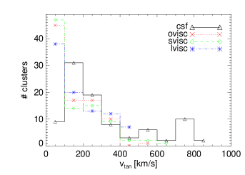
Figure 9: Distribution of rotational velocity (calculated in the region $<0.1R_{500}$) for the Set 1 in the redshift range $[0-0.5]$. The different runs are plotted: csf (solid, black line with triangles), ovisc (dotted, red with crosses), svisc (green, dashed with diamonds), lvisc (blue, dot-dashed with asterisks).

Appendix B Ellipticity of ICM

As interestingly suggested in a recent work by Lau et al. (2010), certain observable features of the cluster X–ray emission, like a flattening of cluster shapes, could unveil the presence of rotationally supported gas, especially in the innermost region. Referring to the X–ray surface brightness maps in Fig. 1, we compare here the ellipticity profiles extracted from the maps in the three projections to the rotational velocity profile, for the two cases of study extracted from Set 1 (namely, g51 and g1) at redshift $z=0$. The ellipticity was calculated by means of the IRAF task ellipse and the reported error bars are those obtained by the fitting method. In Fig. 10 the $v_{tan}$ profile is marked by the solid curve for each cluster, while the dotted, dashed and dot–dashed lines refer to the ellipticities from the three projected maps. Let us note that the ellipticity profiles do not extend to the very central part, since the complex structure in the innermost region does not allow for a simple determination of ellipticities. We can conclude that only a mild relation between ellipticity and rotation is found in these clusters and the difference in the trends shown by the rotational velocity profiles is stronger than the difference among the ellipticity profiles of the two clusters. Nevertheless, comparing the csf run (upper panels) to the ovisc run (lower panels) we can confirm that the cluster shape is actually marked by the physics included in the radiative run, especially in the g1 case, where some rotation establishes in the csf simulation. In conclusion, gas cooling can affect the gas shape by flattening the X–ray isophotes but we do not find a strong significant evidence for that in our case–study clusters, in agreement with the milder rotation found and the nature of such rotational patterns (like in the g1 example), which are likely to be temporary effects driven by major merging events.

Figure 10: Radial profiles of ellipticity (left y–axis; dotted, dashed and dott–dashed curves) for the three projection axis compared with the radial profile of the gas rotational velocity (right y–axis; solid curve). The panels refer to the csf and the ovisc simulations (upper and lower panels, respectively) of g51 (left) and g1 (right) at $z=0$.

References

- Ascasibar & Markevitch (2006) Ascasibar Y., Markevitch M., 2006, ApJ, 650, 102
- Balogh et al. (2001) Balogh M.L., Pearce F.R., Bower R.G., Kay S.T., 2001, MNRAS, 326, 1228
- Binney & Tremaine (2008) Binney J., Tremaine S., 2008, 2nd Ed., Galactic Dynamics, Princeton: Princeton Univ. Press
- Borgani et al. (2006) Borgani S., et al., 2006, MNRAS, 367, 1641
- Borgani & Kravtsov (2009) Borgani S., Kravtsov A.V., 2009, arXiv:0906.4370
- Dolag et al. (2005) Dolag K., Vazza F., Brunetti G., Tormen G., 2005, MNRAS, 364, 753
- Dolag et al. (2009) Dolag K., Borgani S., Murante G., Springel V., 2009, MNRAS, 399, 497
- Fang, Humphrey & Buote (2009) Fang T., Humphrey P., Buote D., 2009, ApJ, 691, 1648
- Inogamov & Sunyaev (2003) Inogamov N.A., Sunyaev R.A., 2003, Astronomy Letters, 29, 791
- Katz & White (1993) Katz N., White S.D.M., 1993, ApJ, 412, 455
- Katz, Weinberg & Hernquist (1996) Katz N., Weinberg D.H., Hernquist L., 1996, ApJS, 105, 19
- Kravtsov, Nagai & Vikhlinin (2005) Kravtsov A.V., Nagai D., Vikhlinin A.A., 2005, ApJ, 625, 588
- Kravtsov, Vikhlinin & Nagai (2006) Kravtsov A.V., Vikhlinin A.A., Nagai D., 2006, ApJ, 650, 128
- Laganá, de Souza & Keller (2009) Laganá T.F., de Souza R.S., Keller G.R., 2010, A&A, 510, A76
- Lin, Mohr & Stanford (2003) Lin Y.T., Mohr J.J., Stanford S.A., 2003, ApJ, 591, 749
- Lau, Kravtsov & Nagai (2009) Lau E.T., Kravtsov A.V., Nagai D., 2009, ApJ, 705, 1129
- Lau et al. (2010) Lau E.T., Nagai D., Kravtsov A.V., Zentner A.R., 2010, arXiv:1003.2270
- McNamara & Nulsen (2007) McNamara B.R., Nulsen P.E.J., 2007, ARA&A, 45, 117
- Markevitch & Vikhlinin (2007) Markevitch M., Vikhlinin A.A., 2007, Phys. Rep., 443, 1
- Mathews & Brighenti (2003) Mathews W.G., Brighenti F., 2003, ARA&A, 41, 191
- Monaghan & Gingold (1983) Monaghan J.J., Gingold R.A., 1983, Journal of Computational Physics, 52, 374
- Monaghan (1997) Monaghan J.J., 1997, Journal of Computational Physics, 136, 298
- Morris & Monaghan (1997) Morris J.P., Monaghan J.J., 1997, Journal of Computational Physics, 136, 41
- Nagai, Vikhlinin & Kravtsov (2007) Nagai D., Vikhlinin A.A., Kravtsov A.V., 2007, ApJ, 655, 98
- Rasia, Tormen & Moscardini (2004) Rasia E., Tormen G., Moscardini L., 2004, MNRAS, 351, 237
- Rasia et al. (2006) Rasia E., et al., 2006, MNRAS, 369, 2013
- Rebusco et al. (2008) Rebusco P., Churazov E.M., Sunyaev R.A., Böhringer H., Forman W., 2008, MNRAS, 384, 1511
- Sarazin (1988) Sarazin C., 1988, X–ray Emission from Clusters of Galaxies, Cambridge: Cambridge Univ. Press
- Schuecker et al. (2004) Schuecker P., Finoguenov A., Miniati F., Böhringer H., Briel U.G., 2004, A&A, 426, 387
- Spergel et al. (2007) Spergel D.N., et al., 2007, ApJS, 170, 377
- Springel, White & Hernquist (2001) Springel V., White M., Hernquist L., 2001, ApJ, 549, 681
- Springel & Hernquist (2003) Springel V., Hernquist L., 2003, MNRAS, 339, 289
- Springel (2005) Springel V., 2005, MNRAS, 364, 1105
- Sunyaev, Norman & Bryan (2003) Sunyaev R.A., Norman M.L., Bryan G.L., 2003, Astronomy Letters, 29, 783
- Tormen, Bouchet & White (1997) Tormen G., Bouchet F.R., White S.D.M., 1997, MNRAS, 286, 865
- Werner et al. (2009) Werner N., Zhuravleva I., Churazov E.M., Simionescu A., Allen S.W., Forman W., Jones C., Kaastra J.S., 2009, MNRAS, 398, 23
- Zhuravleva et al. (2010) Zhuravleva I.V., Churazov E.M., Sazonov S.Y., Sunyaev R.A., Forman W., Dolag K., 2010, MNRAS, 403, 129