Dynamical Black Hole Masses of BL Lac Objects from the Sloan Digital Sky Survey

Abstract

We measure black hole masses for 71 BL Lac objects from the Sloan Digital Sky Survey (SDSS) with redshifts out to $z\sim 0.4$. We perform spectral decompositions of their nuclei from their host galaxies and measure their stellar velocity dispersions. Black hole masses are then derived from the black hole mass – stellar velocity dispersion relation. We find BL Lac objects host black holes of similar masses, $\sim$10^8.5 ${\rm M_{\sun}}$, with a dispersion of $\pm$0.4 dex, similar to the uncertainties on each black hole measurement. Therefore, all BL Lac objects in our sample have the same indistinguishable black hole mass. These 71 BL Lac objects follow the black hole mass – bulge luminosity relation, and their narrow range of host galaxy luminosities confirm previous claims that BL Lac host galaxies can be treated as standard candles. We conclude that the observed diversity in the shapes of BL Lac object spectral energy distributions is not strongly driven by black hole mass or host galaxy properties.

1 Introduction

BL Lac objects are a very rare class of Active Galactic Nuclei (AGNs) thought to be unified with Fanaroff-Riley I (FR I, Fanaroff & Riley 1974) radio galaxies viewed nearly along the axis of a relativistic jet (e.g., see Blandford & Rees 1978; Urry & Padovani 1995). BL Lac objects are among the brightest radio, X-ray, and gamma-ray sources in the entire sky, they are highly polarized ($>$2–3%), and their multiwavelength emission is variable on timescales ranging from minutes to decades (e.g., see Kollgaard 1994; Urry & Padovani 1995). Perhaps the most striking property of BL Lac objects is their optical spectra, which are devoid of strong emission lines because radiation from the Doppler boosted jet is so dominant.

Black hole mass measurements for a large number of BL Lac objects would have a wide range of applications – from investigations aimed toward a better understanding of BL Lac statistical properties, to studies focusing more generally on relativistic jets. For example, AGNs are powered by accretion onto a supermassive black hole, making black hole mass a fundamental parameter – i.e., it sets an AGN’s upper luminosity limit, and it determines the temperature of the accretion disc. Also, BL Lac spectral energy distributions (SEDs) are dominated by jet emission, so they are excellent probes of relativistic jet physics. BL Lac objects show impressively diverse SEDs from object to object, with a synchrotron cutoff occurring anywhere from the near-infrared to the soft-X-ray wavebands (e.g., see Padovani & Giommi 1995). A large sample of black hole masses can thus be used to investigate if black hole mass or another parameter(s) is the primary driver of a jet’s SED (e.g., see Ghisellini & Tavecchio 2008). Even more generally, a sample of BL Lac objects with well determined black hole masses could be incorporated in studies on the scaling of relativistic jets with mass, through, for example, comparison with X-ray binaries in the hard spectral state (e.g., see Merloni et al. 2003; Falcke et al. 2004).

The weak-lined nature of BL Lac spectra, however, introduces unique challenges for obtaining reliable black hole mass measurements. For other classes of AGN, black hole masses can be derived by measuring the widths of gas emission lines and by measuring the continuum luminosity – here, one assumes the gas in the broad emission line region is virialized and adopts a relation between continuum luminosity and size of the broad emission line region (e.g., see Kaspi et al. 2000). However, this technique cannot be employed for AGN with featureless spectra. Even if weak emission is detected (and if one assumes correlations between emission line strength and black hole mass extend to weak emission), the resultant BL Lac black hole masses will be unreliable unless the continuum luminosity is corrected for Doppler boosting. Other techniques for weighing BL Lac central black holes should be seeked.

An alternative method utilizes the dynamics of the stars near a galaxy’s center, i.e., ‘dynamical’ mass estimates. This is done by measuring the line-of-sight stellar velocity dispersion ($\sigma$) from the widths of stellar absorption features, which are Doppler broadened due to the stars’ motions. Thus, if one can decompose an AGN’s host galaxy from the central point source and measure $\sigma$, then black hole masses can be estimated from empirical correlations (the $M_{\rm BH}$–$\sigma$ relation, e.g., see Ferrarese & Merritt 2000; Gebhardt et al. 2000; Tremaine et al. 2002). Black hole masses can also be estimated from the host galaxy’s luminosity (e.g., Kormendy & Richstone 1995; Magorrian et al. 1998), and sizable samples of BL Lac black hole masses ($\sim$60-120 objects) have indeed been derived in such a way (e.g., Wu et al. 2009; Xu et al. 2009). However, the black hole mass – galaxy luminosity correlation is not as tight as the $M_{\rm BH}$–$\sigma$ relation, and black hole masses derived from galaxy luminosities can sometimes be overestimated by up to two orders of magnitude (e.g., see Ferrarese & Merritt 2000).

Given the above considerations, we prefer to estimate black hole masses using stellar velocity dispersions. However, in the past, there was not an abundant supply of BL Lac objects with high-quality spectra with enough apparent host galaxy light to perform the requisite measurements of $\sigma$. For this reason, subsets of BL Lac objects with dynamical black hole estimates tend to contain at most $\sim$30 objects (e.g., see Falomo et al. 2003; Woo et al. 2005). Fortunately, relatively large BL Lac samples containing hundreds of objects have recently come online (e.g., Turriziani et al. 2007; Massaro et al. 2009). Here, we use the 723 object BL Lac sample assembled from the Sloan Digital Sky Survey (SDSS, York et al. 2000) by Plotkin et al. (2010, hereafter P10). Each object has a high-quality SDSS spectrum, and the sheer size of this sample ensures a relatively large number of BL Lac spectra show a strong enough host galaxy component to measure $\sigma$. We attempt black hole mass measurements for 143 P10 BL Lac objects, for which we derive 71 black hole masses. Leon-Tavares et al. (2010) recently presented a similarly sized sample of dynamical black hole masses from our older radio-selected BL Lac catalog (Plotkin et al. 2008). In §2 we describe the parent BL Lac sample, and we explain our algorithm for estimating black hole masses in §3. The measured distribution of black hole masses and host galaxy luminosities are discussed in §4, and we comment on the import of black hole mass in determining the shape of BL Lac SEDs. Finally, our conclusions are summarized in §5. Throughout, we adopt $H_{0}=71$ km s^-1 Mpc^-1, $\Omega_{m}=0.27$, and $\Omega_{\Lambda}=0.73$.

2 The BL Lac Sample

The P10 optically selected BL Lac sample contains 723 objects from 8250 deg² of SDSS spectroscopy. About 75% of these BL Lac objects were discovered by the SDSS. In order for a source to be retained as a BL Lac candidate, its SDSS spectrum cannot show any emission line with rest-frame equivalent width (REW) stronger than 5 Å, and its Ca II H/K depression must be smaller than 40%. There is no explicit requirement for an object to be a radio or X-ray emitter, but the sample was correlated post-selection with the NRAO VLA Sky Survey (NVSS, Condon et al. 1998) and with the Faint Images of the Radio Sky at Twenty-cm (FIRST, Becker et al. 1995) radio surveys, as well as with the ROSAT All Sky Survey (RASS Voges et al. 1999, 2000) in the X-ray. We refer the reader to P10 for details.

About one-third of SDSS BL Lac objects have spectroscopic redshifts derived from host galaxy spectral features in their SDSS spectra. Here, we limit ourselves to 143 spectra that have reliable spectroscopic redshifts in P10, that match to a FIRST and/or NVSS radio source and are radio-loud (i.e., radio-to-optical flux ratio is larger than 10, see Kellermann et al. 1989; Stocke et al. 1992), and that have $z<0.4$. Objects with $z>0.4$ are too distant to show significant host galaxy radiation in their SDSS spectra. We attempt to measure black hole masses for each of these 143 BL Lac objects. These 143 objects are among the most weakly beamed BL Lac objects in P10 (or else they would not show a host galaxy component in their optical spectra), thereby minimizing orientation effects.

3 Black Hole Mass Measurements

To measure black hole masses we first remove the contribution from the AGN to the observed spectrum (§3.1), and we then measure the line of sight stellar velocity dispersion ($\sigma$) in each decomposed host galaxy spectrum (§3.2). We assess the reliability of the spectral decompositions in §3.3, and in that section we identify 72 spectra with unreliable decompositions (most have poor fits based on their reduced $\chi^{2}$). Finally, we estimate black hole masses and host galaxy luminosities for the other 71 spectra (§3.4 and 3.5, respectively).

3.1 Spectral Decomposition

We assume each SDSS spectrum is a combination of two components: the thermal contribution from the host galaxy, and the non-thermal emission from the relativistic jet. We model the latter as a power law: $f_{\nu}=f_{\nu_{0}}\left(\nu/\nu_{0}\right)^{-\alpha_{\nu}}$, where $\alpha_{\nu}$ is the spectral index and $f_{\nu_{0}}$ is the flux density at reference frequency $\nu_{0}$. We choose $\nu_{0}$=c/(6165 Å), which is the reference frequency of the SDSS $r$ filter. To find the best fit power-law and host galaxy parameters, we make slight modifications to the Gas And Absorption Line Fitting algorithm (GANDALF), as described below.

GANDALF iteratively fits an observed galaxy spectrum with combinations of stellar templates convolved by the best-fit line of sight velocity dispersion; it also simultaneously fits a user defined list of gas emission lines, modeling the lines with Gaussian templates. The Penalized Pixel-Fitting method (pPXF, see §3.2) of Cappellari & Emsellem (2004) is used by GANDALF to provide initial guesses for the stellar continuum fits and velocity dispersions. Nonlinear fits are then performed with the Bounded-Variables Least-Squares algorithm (BVLS) and with Levenberg-Marquardt least-squares minimization (see Markwardt 2009). An important feature of GANDALF is that it fits the stellar continuum and gas emission simultaneously, instead of masking spectral regions containing emission lines from the continuum fits. This technique is likely to yield less biased stellar continua (see Sarzi et al. 2006).

We modified GANDALF to also include a power law component from the AGN, and we then ran the modified code on the 143 BL Lac objects showing a host galaxy component in their SDSS spectra. All fits are performed in the rest-frame. The power law is constrained to always be positive and to not account for more than 80% of the observed flux at 3900 Å. The latter constraint is to ensure the power law is physically meaningful: if the power law accounted for all of the observed flux, then we would not see any contribution from the host galaxy to the BL Lac spectrum. We use stellar population models (Vazdekis et al. 2010) based on the Medium-resolution Isaac Newton Telescope library of empirical spectra (MILES, Sánchez-Blázquez et al. 2006), and the SDSS BL Lac spectra are convolved to match the spectral resolution of the MILES templates (81 km s^-1). Because BL Lac emission lines are by definition very weak, we only fit gas emission for [O II], [O III], H$\beta$, H$\alpha$, [N II], and [S II], and we exclude spectral regions containing Oxygen sky lines from the fits. Sample spectral decompositions are shown in Fig. 1.

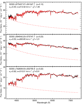
Figure 1: Three sample SDSS spectra, in their rest-frames, convolved to the MILES spectral resolution, shown as black solid lines. The best GANDALF fits are overdrawn as red solid lines, and the red dashed lines illustrate the power law components. This figure appears in color in the online version of this article.

3.2 Velocity Dispersion Measurements

For each BL Lac spectrum, we subtract the best fit power law and emission lines, yielding a spectrum of just the host galaxy. We then measure the host galaxy’s velocity dispersion, $\sigma$, with the pPXF method. The pPXF algorithm fits galaxy spectra by convolving sets of stellar templates with a best-fit velocity dispersion. We again use the MILES stellar templates, and we adopt the best-fit combination of stellar templates found during the GANDALF spectral decomposition in §3.1. Since we remove any (weak) emission lines from our host galaxy spectra, there is no need to mask out regions of the spectra containing gas emission. We do, however, still omit regions covering Oxygen sky lines from the pPXF fits.

We estimate errors on $\sigma$ via Monte Carlo simulations (see Cappellari & Emsellem 2004). For each pixel’s flux density, $f_{\lambda,i}$, we add noise $\pm\epsilon_{i}$, where $\epsilon_{i}$ is drawn randomly from a normal distribution with standard deviation equal to each pixel’s flux density measurement error. We then remeasure the velocity dispersion with pPXF, repeating 100 times. We adopt the standard deviation in the 100 velocity dispersion measurements as the formal uncertainty on $\sigma$, which is typically better than 10%. Uncertainties on power law indices are similarly derived by randomly adding noise and re-running GANDALF 100 times per spectrum. The best-fit stellar velocity dispersions and their uncertainties are included in Table 1.

In Table 1 we also include the best fit power law indices, $\alpha_{\nu}$, and the fraction of the observed flux density accounted for by the power law at rest-frame 6165 Å, $f_{pl}$. The measured values of $\alpha_{\nu}$ are typical for BL Lac objects, with an average $\left<\alpha_{\nu}\right>=0.70\pm 0.56$. The recovered values of $f_{pl}$ (with an average value $0.34\pm 0.12$) are as expected. If the power law is too weak it would not be a BL Lac object, and if the power law is too strong the host galaxy would not be seen in the optical spectrum. The fraction of light accounted for by the power law is systematically higher if the calculation is instead done at a wavelength bluer than 6165 Å.

Table 1: Black Hole Masses and Other Measured Parameters

Name	RA	Dec	Redshift	$\alpha_{\nu}$	$\sigma_{\alpha_{\nu}}$	$f_{pl}$a	$\sigma_{\star}$	$\sigma_{\sigma_{\star}}$	$\log M_{\rm BH}$	$\sigma_{M_{\rm BH}}$	$M_{hg}$	$\sigma_{M_{hg}}$
(SDSS J)	(deg.)	(deg.)					(km s-1)	(km s-1)	(${\rm M_{\sun}}$)	(dex)	(mag)	(mag)
002200.95$+$000657.9	5.50396	0.11610	0.306	0.55	0.21	0.16	246	13	8.49	0.32	-22.42	0.14
005620.07$-$093629.7	14.08366	-9.60826	0.103	0.80	0.05	0.33	332	9	9.01	0.32	-23.26	0.30
075437.07$+$391047.7	118.65446	39.17994	0.096	0.43	0.28	0.29	213	5	8.24	0.31	-22.95	0.08
080018.79$+$164557.1	120.07831	16.76588	0.309	1.40	0.15	0.47	259	13	8.58	0.32	-23.17	0.32
082323.24$+$152447.9	125.84686	15.41333	0.167	0.50	0.14	0.23	293	12	8.80	0.32	-22.76	0.05
082814.20$+$415351.9	127.05917	41.89776	0.226	1.12	0.04	0.27	299	9	8.83	0.32	-23.04	0.30
083417.58$+$182501.6	128.57328	18.41712	0.336	0.54	0.35	0.18	399	37	9.34	0.36	-22.87	0.32
083548.14$+$151717.0	128.95059	15.28808	0.168	1.14	0.14	0.53	179	14	7.94	0.33	-22.76	0.31
083918.74$+$361856.1	129.82812	36.31559	0.335	0.61	0.11	0.20	247	27	8.50	0.36	-22.61	0.34
084712.93$+$113350.2	131.80388	11.56396	0.198	-0.22	0.19	0.35	251	15	8.52	0.32	-22.87	0.09
085036.20$+$345522.6	132.65085	34.92296	0.145	0.76	0.11	0.33	263	8	8.61	0.31	-23.19	0.05
085729.78$+$062725.0	134.37411	6.45695	0.338	-0.45	0.71	0.09	212	21	8.23	0.35	-22.70	0.36
085749.80$+$013530.3	134.45751	1.59176	0.281	0.54	0.17	0.37	276	13	8.69	0.32	-23.91	0.10
090207.95$+$454433.0	135.53316	45.74250	0.289	1.07	0.01	0.48	291	11	8.78	0.32	-22.43	0.33
090314.70$+$405559.8	135.81128	40.93330	0.188	0.37	0.09	0.20	218	8	8.28	0.31	-23.09	0.07
090953.28$+$310603.1	137.47201	31.10088	0.272	-0.56	0.41	0.21	321	16	8.95	0.32	-23.78	0.31
091045.30$+$254812.8	137.68876	25.80358	0.384	1.30	0.02	0.41	249	31	8.51	0.38	-22.82	0.36
091651.94$+$523828.3	139.21642	52.64121	0.190	0.66	0.05	0.34	252	7	8.53	0.31	-23.68	0.07
093037.57$+$495025.6	142.65655	49.84045	0.187	0.41	0.15	0.41	244	20	8.48	0.34	-22.64	0.31
094022.44$+$614826.1	145.09354	61.80727	0.211	0.85	0.09	0.33	258	13	8.57	0.32	-22.48	0.08
094542.23$+$575747.7	146.42599	57.96325	0.229	0.53	0.09	0.44	266	14	8.63	0.32	-23.39	0.30
101244.30$+$422957.0	153.18461	42.49918	0.365	0.47	0.35	0.47	272	25	8.67	0.35	-23.03	0.28
102453.63$+$233234.0	156.22348	23.54278	0.165	1.06	0.04	0.51	137	9	7.46	0.33	-22.83	0.30
102523.04$+$040228.9	156.34603	4.04139	0.208	1.23	0.08	0.44	206	16	8.18	0.33	-22.26	0.31
103317.94$+$422236.3	158.32478	42.37678	0.211	0.75	0.08	0.20	260	8	8.59	0.31	-22.91	0.05
104029.01$+$094754.2	160.12090	9.79839	0.304	0.42	0.01	0.35	277	13	8.70	0.32	-23.05	0.31
104149.15$+$390119.5	160.45480	39.02209	0.208	1.01	0.10	0.22	255	11	8.55	0.32	-23.41	0.06
104255.44$+$151314.9	160.73103	15.22083	0.307	1.23	0.17	0.55	166	33	7.81	0.46	-22.16	0.35
105344.12$+$492955.9	163.43387	49.49889	0.140	1.31	0.04	0.42	244	9	8.47	0.31	-23.13	0.05
105538.62$+$305251.0	163.91095	30.88085	0.243	0.81	0.12	0.20	238	17	8.43	0.33	-22.72	0.31
105606.61$+$025213.4	164.02756	2.87041	0.236	1.13	0.13	0.37	197	11	8.11	0.32	-22.58	0.31
105723.09$+$230318.7	164.34625	23.05522	0.378	0.83	0.17	0.37	223	19	8.32	0.34	-23.17	0.24
112059.74$+$014456.9	170.24892	1.74914	0.368	0.14	0.21	0.20	465	18	9.60	0.33	-22.96	0.34
113630.09$+$673704.3	174.12539	67.61789	0.134	1.14	0.04	0.44	221	7	8.30	0.31	-22.65	0.05
114023.48$+$152809.7	175.09784	15.46937	0.244	-0.38	0.14	0.30	428	32	9.46	0.35	-23.96	0.09
114535.10$-$034001.4	176.39625	-3.66708	0.168	-0.48	0.29	0.14	216	9	8.27	0.31	-22.78	0.07
115404.55$-$001009.8	178.51899	-0.16941	0.254	0.45	0.07	0.37	228	16	8.36	0.33	-22.53	0.31
115709.53$+$282200.7	179.28974	28.36687	0.300	0.56	0.14	0.26	369	21	9.20	0.33	-23.52	0.10
120837.27$+$115937.9	182.15533	11.99387	0.369	0.66	0.14	0.45	271	22	8.66	0.34	-23.35	0.34
123123.90$+$142124.4	187.84962	14.35680	0.256	1.64	0.03	0.71	264	33	8.62	0.38	-22.72	0.32
123131.39$+$641418.2	187.88081	64.23841	0.163	-0.16	0.05	0.25	300	8	8.84	0.31	-23.37	0.30
123831.24$+$540651.8	189.63018	54.11441	0.224	1.07	0.07	0.30	263	12	8.61	0.32	-23.09	0.06
125300.95$+$382625.7	193.25398	38.44049	0.371	1.09	0.41	0.41	214	7	8.24	0.31	-22.36	0.37
131330.12$+$020105.9	198.37552	2.01832	0.356	0.98	0.01	0.45	248	28	8.50	0.36	-22.96	0.36
132231.46$+$134429.8	200.63112	13.74164	0.377	0.51	0.29	0.28	323	17	8.97	0.33	-23.25	0.33
132239.31$+$494336.2	200.66380	49.72673	0.332	0.26	0.26	0.15	273	24	8.67	0.35	-23.00	0.19
132301.00$+$043951.3	200.75419	4.66427	0.224	0.37	0.12	0.22	304	14	8.86	0.32	-23.17	0.30
132617.70$+$122958.7	201.57378	12.49965	0.204	0.30	0.11	0.25	266	13	8.63	0.32	-22.87	0.31
133612.16$+$231958.0	204.05067	23.33280	0.267	0.30	0.19	0.31	256	16	8.56	0.33	-22.80	0.32
134105.10$+$395945.4	205.27127	39.99595	0.172	1.52	0.03	0.50	244	13	8.48	0.32	-22.43	0.31
134136.23$+$551437.9	205.40096	55.24388	0.207	0.86	0.06	0.38	219	15	8.29	0.33	-22.71	0.31
134633.98$+$244058.4	206.64162	24.68291	0.167	0.81	0.05	0.32	219	11	8.29	0.32	-22.29	0.06
135314.08$+$374113.9	208.30870	37.68721	0.216	1.11	0.05	0.36	291	10	8.79	0.32	-23.64	0.10
140350.28$+$243304.8	210.95951	24.55133	0.343	1.76	0.45	0.57	233	37	8.39	0.41	-22.22	0.39
142421.17$+$370552.8	216.08824	37.09802	0.290	2.38	0.89	0.53	233	11	8.39	0.32	-23.21	0.22
142832.60$+$424021.0	217.13587	42.67252	0.129	-0.21	0.14	0.30	277	11	8.70	0.32	-23.19	0.05
144248.28$+$120040.2	220.70118	12.01119	0.163	-0.20	0.14	0.31	319	15	8.94	0.32	-23.27	0.30
144932.70$+$274621.6	222.38626	27.77269	0.227	0.66	0.09	0.33	303	18	8.86	0.33	-22.85	0.31
153311.25$+$185429.1	233.29688	18.90809	0.307	0.59	0.18	0.44	312	13	8.91	0.32	-23.01	0.32
155412.07$+$241426.6	238.55032	24.24073	0.301	0.05	0.31	0.21	260	16	8.59	0.33	-22.81	0.16
155424.12$+$201125.4	238.60054	20.19040	0.222	0.50	0.11	0.29	317	9	8.94	0.32	-23.48	0.05
160118.96$+$063136.0	240.32900	6.52667	0.358	1.06	0.01	0.41	276	11	8.69	0.32	-23.06	0.33
160519.04$+$542059.9	241.32937	54.34998	0.212	0.67	0.11	0.33	171	18	7.85	0.36	-21.86	0.32
161541.21$+$471111.7	243.92174	47.18661	0.199	1.31	0.03	0.45	204	10	8.17	0.32	-22.72	0.30
161706.32$+$410647.0	244.27636	41.11307	0.267	1.76	0.03	0.61	169	11	7.84	0.33	-22.79	0.31
162839.03$+$252755.9	247.16263	25.46553	0.220	0.92	0.06	0.32	310	9	8.90	0.32	-23.06	0.05
163726.66$+$454749.0	249.36112	45.79695	0.192	1.27	0.07	0.29	237	10	8.42	0.31	-22.44	0.05
164419.97$+$454644.3	251.08321	45.77900	0.225	0.85	0.06	0.32	288	13	8.76	0.32	-23.06	0.30
205456.85$+$001537.7	313.73690	0.26049	0.151	0.15	0.32	0.23	272	8	8.67	0.31	-22.63	0.22
205938.57$-$003756.0	314.91071	-0.63222	0.335	0.68	0.01	0.31	114	2	7.16	0.32	-22.84	0.32
223301.11$+$133602.0	338.25465	13.60056	0.214	0.27	0.26	0.29	253	14	8.54	0.32	-22.67	0.31

3.3 Assessing the Quality of the Decomposition

There are several reasons why some of the spectral decompositions might fail. All 143 SDSS BL Lac spectra are of high enough quality to derive redshifts from host galaxy spectral features, and to allow reliable BL Lac classifications. However, the amount of the host galaxy flux for the most highly beamed objects in this subset is not strong enough to obtain accurate spectral decompositions, and some other objects do not have high enough signal-to-noise. We thus exclude 54 objects with reduced $\chi^{2}_{r}>2$ (each GANDLAF fit has $\sim$4200 degrees of freedom), and we remove an additional 12 objects for which the spectral decompositions did not converge, or the error on the velocity dispersion is larger than 40 km s^-1 (i.e., half the spectral resolution of the MILES stellar templates). Upon visual examination of each spectral fit, we remove an additional six objects with poor fits. Most of these six objects have Ca II H/K break strengths smaller than 15%, and their continua are too dominated by the power law to obtain reliable $\sigma$ measurements. We are left with 71 spectra for which we determine black hole masses. For the remainder of this paper we only consider these 71 objects.

The 71 successfully decomposed objects are clearly biased toward those with strong host galaxy components. The amount of stellar flux in BL Lac spectra depends primarily on orientation. That is, more weakly beamed BL Lac objects show more stellar light (e.g., Landt et al. 2002; Plotkin et al. 2008), and our 71 object subset is therefore biased toward larger viewing angles. All of the 71 BL Lac objects with successful decompositions have Ca II H/K breaks stronger than 15%, roughly translating to viewing angles larger than about 15-25 deg (see Fig. 8 of Landt et al. 2002). Since the above bias is primarily geometric, we make the reasonable assumption that our analysis and conclusions on this subset can be extrapolated to the entire BL Lac population.

As pointed out by Woo et al. (2005), less massive black holes live in less luminous galaxies and are therefore more difficult to measure since the host galaxy is harder to see, especially at increasing redshift. This selection effect could artificially narrow the observed stellar velocity (and therefore black hole mass) distribution. We however do not see any correlation between velocity dispersion and redshift in our sample of 71 objects, and there is no obvious deficit of low mass black holes at high-redshift. We therefore do not believe this strongly affects our sample. Regardless, since we do not attempt to derive a complete sample of BL Lac objects with black hole masses here, this potential bias will not alter our conclusions.

3.4 Measuring Black Hole Masses

The $M_{\rm BH}$–$\sigma$ relation is parameterized as

$$\log\left(M_{\rm BH}/{\rm M_{\sun}}\right)=\alpha+\beta\log\left(\sigma/\sigma_{0}\right),$$ (1)

with $\sigma_{0}=200$ km s^-1. We use the coefficients derived by Tremaine et al. (2002) from a sample of 31 nearby galaxies: $\alpha=8.13\pm 0.06$ and $\beta=4.02\pm 0.32$. To estimate error bars, we propagate the uncertainties on our velocity dispersion measurements and the errors on $\alpha$ and $\beta$. We add that uncertainty in quadrature with the $M_{\rm BH}$–$\sigma$ relation’s intrinsic scatter in $\log M_{\rm BH}$: $\sigma_{\rm int}\sim\pm 0.30$ dex (see Tremaine et al. 2002). Typical error bars on our black hole measurements, including the intrinsic scatter of the $M_{\rm BH}-\sigma$ relation, are $\pm$0.30–0.35 dex. The measured black hole mass distribution is shown in Fig 2, and masses are listed along with the other fitted parameters (i.e., power law indices, velocity dispersions, etc.) in Table 1.

There appears to be a small number of black hole mass measurements that deviate from the mean black hole mass in Figure 2 (i.e., $\log M_{\rm BH}<7.5$ and $\log M_{\rm BH}>9.0$). We re-examined their spectral decompositions visually, and we find no compelling reason to remove them from the sample. Instead, we attribute those points to populating the high and low sigma tails of the mass distribution, and to small number statistics. A Kolmogorov-Smirnoff test shows our measured black hole mass distribution is consistent with a Gaussian, in which case we would expect 3.6 black hole mass measurements to deviate from the mean by $\pm$2$\sigma$. Indeed, four black hole mass measurements populate the 2$\sigma$ tail.

Figure 2: Distribution of black hole mass measurements, derived with Equation 1.

3.5 Measuring Host Galaxy Luminosities

After performing the spectral decomposition we are able to construct spectra of each BL Lac object’s host galaxy. We use these spectra to estimate the absolute magnitude each host galaxy would have in the Cousins $R_{c}$ filter at $z=0$. First, we measure the host galaxy flux at rest-frame 6581 Å (the effective wavelength of the $R_{c}$ filter), and we then apply a bandpass correction and correct for extinction from the Milky Way (using the dust maps of Schlegel et al. 1998).

The 3^′′ apertures of each SDSS spectroscopic fiber does not include all of the host galaxy’s flux, and an aperture correction must be applied. To determine the fraction of light covered by each spectroscopic fiber, we perform an image decomposition on each source’s sdss $i$ filter image using the GALFIT software (Peng et al. 2002). We model each BL Lac object with a point source, and a de Vaucouleur profile (BL Lac objects probably live exclusively in elliptical galaxies, Urry et al. 2000). We are able to measure the half light effective radius $r_{e}$ for 29 BL Lac hosts, requiring $r_{e}>3$ pix, and that the best-fit host galaxy and central point source models are centered on the same coordinates. We adopt these $r_{e}$ values to calculate the aperture correction for these 29 objects. For the remaining objects, we assume $r_{e}=10$ kpc, the median effective radius for the 29 objects. This value is also consistent with the median effective radius from other BL Lac host galaxy studies (e.g., Urry et al. 2000).

The above aperture correction contributes the largest source of uncertainty to our luminosity estimates. For the 29 objects with $r_{e}$ measurements, the uncertainties on $r_{e}$ are typically of the order $\pm$1 kpc (0.6 pix), introducing typical errors on the host galaxy absolute magnitudes of $\pm$0.06 mag. The systematic error introduced for the other 42 objects by assuming $r_{e}=10$ kpc is more severe. To estimate the uncertainty, we calculate the host galaxy luminosity for the 29 objects with $r_{e}$ measurements by assuming $r_{e}=10$ kpc, and we compare to the host galaxy luminosity estimates using each $r_{e}$ measurement. There is no systematic offset between the two absolute magnitude measurements; however, the measurements disagree with a standard deviation of $\pm$0.3 mag. We therefore adopt a systematic uncertainty of $\pm$0.3 mag for the 42 objects without $r_{e}$ measurements. Note, the error’s dependence on redshift is weak for $z>0.1$.

We add the above uncertainties in quadrature to the statistical errors estimated from Monte Carlo simulations, where we randomly added noise to each spectrum and re-ran each spectral decomposition 100 times (as described in §3.2). These uncertainties, including error from the aperture corrections, are listed in Table 1. For the 29 objects with $r_{e}$ measurements, we do not estimate absolute magnitudes using the total integrated host galaxy apparent magnitude from their best-fit de Vaucouleur profiles because the required K-corrections would introduce additional uncertainties.

4 Discussion

4.1 Black Hole Masses

We measure an average black hole mass of $\left<\log M_{\rm BH}\right>=8.54\pm 0.047~{}{\rm M_{\sun}}$ (the quoted uncertainty is the error of the mean), with a standard deviation of $\pm$0.40 dex. The dispersion in the distribution of black hole masses is comparable to the typical measurement error of $\pm$0.30–0.35 dex. Thus, it is possible that the observed spread of black hole masses can be attributed only to measurement error, and we conclude BL Lac black hole masses are virtually indistinguishable.

Our black hole estimates are consistent with those in the literature. For example, Falomo et al. (2003) find $\left<\log M_{\rm BH}\right>=8.57~{}{\rm M_{\sun}}$ for a sample 12 BL Lac objects with dynamical black hole mass measures. Woo et al. (2005) find 32 BL Lac objects with dynamical black hole mass measures to have a dispersion from $4\times 10^{7}-6\times 10^{8}~{}{\rm M_{\sun}}$, and $\left<\log M_{\rm BH}\right>\sim 8.30~{}{\rm M_{\sun}}$. They note, however, that their sample is relatively shallow ($\left<z\right>\sim 0.17$), and it thus may not probe a large enough volume to recover a substantial number of massive central black holes. Indeed, when they include an additional $\sim$30 BL Lac objects with black hole mass measures based on host galaxy luminosity, their $\sim$60 object sample has $\left<z\right>\sim 0.31$ and a dispersion in black hole mass measures that extends to $4\times 10^{9}~{}{\rm M_{\sun}}$ (identical to the largest black hole mass measured in our 71 object sample).

It is interesting that the black hole mass distribution is so narrow, because BL Lac SEDs can be incredibly diverse: BL Lac objects are often classified as high-energy peaked (HBL) or low-energy peaked (LBL) BL Lac objects, depending on the cutoff frequency of their synchrotron radiation (see Padovani & Giommi 1995). Nieppola et al. (2006) show BL Lac synchrotron radiation cutoff frequencies can span close to ten orders of magnitude from object to object. Yet, we find that differences in SED shapes must not significantly depend on black hole mass.

Figure 3: Logarithm of black hole mass vs. logarithm of the ratio of radio (5 GHz) to X-ray (1 keV) specific luminosities. The latter parameterizes the shape of each object’s SED. Error bars are omitted for clarity – a typical (1$\sigma$) black hole mass measurement error is shown in the top left corner. The measurement errors on $\log\left(L_{r}/L_{X}\right)$ are smaller than the data points. We do not observe a significant correlation indicating one or more parameters other than black hole mass are important for determining the SED shape.

We parameterize the SED shape of our 71 BL Lac objects with $\log\left(L_{r}/L_{X}\right)$, where $L_{r}$ and $L_{X}$ are the specific luminosities (in erg s^-1 Hz^-1) at rest-frames 5 GHz and 1 keV respectively, and their values are taken from P10. The SEDs of BL Lac objects with smaller $L_{r}/L_{X}$ values have synchrotron cutoffs at higher frequencies. We follow Plotkin et al. (2008) and classify objects with $\log\left(L_{r}/L_{X}\right)<5.76$ as HBLs. Our sample of 71 BL Lac objects includes 59 HBLs and 12 LBLs; the relatively larger number of HBLs in our sample is an artifact of SDSS BL Lac selection (see P10, ). A Kolmogorov-Smirnoff test indicates a p=0.47 chance that the HBL and LBL black hole mass distributions come from the same population, and their black hole mass distributions are therefore not statistically different.

The logarithm of black hole mass vs. $\log\left(L_{r}/L_{X}\right)$ is shown in Fig. 3, and we see no statistically significant correlation. The linear Pearson correlation coefficient between $\log\left(L_{r}/L_{x}\right)$ and $\log M_{\rm BH}$ is $r=0.018$, with a probability $p=0.44$ of randomly finding a stronger correlation, treating $L_{r}/L_{X}$ limits as exact. We find $r=0.036$ and $p=0.40$ if we only consider the 55 objects with X-ray detections in RASS. Thus, differences between BL Lac SEDs are likely not driven solely by black hole mass. This is consistent with Ghisellini & Tavecchio (2008), who show the observed range of BL Lac synchrotron cutoff frequencies can be replicated by assuming all BL Lac objects have the same black hole masses and varying only their Eddington normalized accretion rates (see their Fig. 5). We do not derive normalized accretion rates for the 71 BL Lac objects with black hole mass measurements here because, without knowing their Doppler factors, we cannot accurately debeam their luminosities.

4.2 Host Galaxies

A correlation between black hole mass and host galaxy absolute magnitude ($M_{R_{c}}$) is found (Fig. 4), confirming that BL Lac objects follow the black hole mass – bulge relationship (e.g., Kormendy & Richstone 1995). Our sample contains the largest number of BL Lac objects for which the correlation has been tested. We perform a linear regression using the technique of Kelly (2007), which takes a Bayesian approach and accurately accounts for measurement errors in both variables. We find $\log\left(M_{BH}/M_{\sun}\right)=\left(-4.12\pm 2.99\right)-\left(0.55\pm 0.13\right)M_{R_{c}}$, and a linear Pearson’s correlation coefficient $r=-0.513$ ($p<10^{-5}$ chance of randomly finding a stronger correlation). Our regression agrees with the correlation found by McLure & Dunlop (2002) for a sample of 90 active and inactive galaxies covering similar redshift ranges and host galaxy luminosities (dashed line in Fig. 4).

There are a small number of points that deviate from the black hole mass - bulge relation in Fig. 4 (i.e., those with $\log M_{\rm BH}<7.5$ and $\log M_{\rm BH}>9.0$). There is no motivation to remove those objects from our sample based on the quality of their spectral decompositions, and we thus include all objects in the above regression. We however note they merit further study.

There is no reason to assume the observed correlation is driven by correlated errors between our BL Lac black hole mass and host galaxy luminosity measurements. We test this by randomly adding noise to each observed spectrum and rerunning our spectral decomposition 100 times for each BL Lac object. No source shows a significant correlation between its 100 pairs of $\log M_{\rm BH}$ and $M_{R_{c}}$: the average Pearson’s correlation coefficient for the 71 sources is $\left<r\right>=-0.01$, and no source shows an anti-correlation stronger than $r=-0.2$.

That BL Lac objects obey the same black hole mass – bulge relation as other galaxies indicates that the black hole formation histories of BL Lac objects are similar to other AGN. This is further support that parameters other than black hole mass (such as orientation, accretion rate, etc.), must be important for dictating if an AGN looks like a BL Lac phenomenon, and then for determining if the BL Lac object is an LBL or HBL.

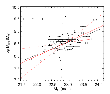
Figure 4: Logarithm of black hole mass vs. host galaxy absolute magnitude in the Cousins $R_{c}$ filter. Error bars on absolute magnitude are shown for the 29 objects with effective radius measurements. For clarity, a typical error bar for the other 42 objects (where we assume $r_{e}=10$ kpc) is shown in the top left corner, as is the typical $1\sigma$ uncertainty for all 71  black hole mass measurements. The solid red line shows our best-fit linear regression using the Bayesian method of Kelly (2007), and the red dotted lines illustrate the $\pm$3$\sigma$ uncertainties. The black hole mass – bulge relationship from McLure & Dunlop (2002) is overplotted as a black dashed line for comparison. This figure appears in color in the online version of this article.

With the black hole mass – bulge relation in mind, we expect a small scatter in the BL Lac host galaxy luminosity distribution, since they have a relatively narrow range of black hole masses. This is indeed observed, as shown in Fig. 5. The BL Lac host galaxies are well fit by a Gaussian with $\left<M_{R_{c}}\right>=-22.9$ mag and a standard deviation of just $\pm$0.4 mag. This confirms the “standard candle” result of Sbarufatti et al. (2005), who showed 64 BL Lac objects with their host galaxies imaged by the Hubble Space Telescope have host galaxy absolute magnitudes well-fit by a Gaussian with mean $-22.8$ mag and standard deviation $\pm$0.5 mag (using the same cosmology employed herein). For the redshifts considered here, the distribution is sufficiently narrow to estimate redshifts better than $\Delta z\sim\pm 0.07$–0.08 (e.g., see Sbarufatti et al. 2005, Meisner & Romani 2010, P10). Meisner & Romani (2010) and P10 apply the standard candle result to show that BL Lac objects lacking spectroscopic redshifts tend to be more distant on average, which can have important implications for understanding BL Lac evolution.

Figure 5: Absolute magnitude of each decomposed host galaxy in the $R_{c}$ filter. The distribution of absolute magnitudes is well described by a Gaussian with mean -22.9 mag and standard deviation $\pm$0.4 mag. This confirms earlier claims that the luminosities of BL Lac host galaxies is narrow enough to treat them as standard candles. We do not see any differences in the host luminosities of LBLs or HBLs, indicating the host galaxy does not play a significant role in determining their SEDs.

We find no significant difference between the distribution of host galaxy luminosities for HBLs and LBLs. The same host galaxy absolute magnitude ($\left<M_{R_{c}}\right>=-22.9$ mag) is measured for both HBLs and LBLs, and the Student’s t-test indicates a probability $p=0.977$ that both distributions have the same mean assuming their variances are similar ($p=0.973$ if we allow for different variances). The Student’s t-test assumes the data follow a normal distribution, which is justified by our observations (see Fig. 5). Even if we drop this assumption, the non-parametric Mann-Whitney U-Test still indicates the sample means are not significantly different (at the $p=0.379$ level). Finally, a Kolmogorov-Smirnoff test gives a $p=0.820$ chance the samples are drawn from the same parent population. We thus conclude that the observed diversity in BL Lac SEDs is not caused by differences in host galaxy properties.

5 Conclusions

AGN very likely influenced the formation of galaxies and heirarchical structure in the universe (e.g., di Matteo et al. 2005); obtaining reliable AGN black hole mass estimates is therefore an important endeavor. We presented dynamical black hole mass measurements for 71 BL Lac objects that show enough host galaxy contribution to their SDSS spectra to measure their stellar velocity dispersions.

We find SDSS BL Lac objects have similar black hole masses, with the dispersion in their distribution comparable to the measurement uncertainty ($\sim$0.30–0.35 dex). We do not see any trend between black hole mass and the ratio of radio to X-ray luminosity, which serves as a proxy for SED shape. Our conclusion is that the diverse SED shapes exhibited by BL Lac objects is not controlled solely by black hole mass; another parameter, perhaps accretion rate, must be important (e.g., see Ghisellini & Tavecchio 2008). Dynamical black hole mass measures can only be obtained for the most weakly beamed BL Lac objects, or else their optical spectra do not show a strong enough host galaxy component. Therefore, the 71 BL Lac objects with black hole measures have similar orientation angles, and relativistic beaming is likely secondary in determining the shape of their SEDs. However, orientation effects may not be completely negligible (e.g., see Nieppola et al. 2008).

We also recover a correlation between black hole mass and host galaxy luminosity that is consistent with the black hole mass – bulge luminosity relation in the literature (e.g., McLure & Dunlop 2002). This indicates the formation histories of BL Lac central black holes is similar to other AGN; we do not see any evidence that SED shape depends on host galaxy properties either. Our host galaxy decomposition also supports claims that the distribution of BL Lac host galaxy luminosities is narrow enough to treat them as standard candles. One can thus derive “imaging redshifts” for BL Lac objects lacking spectroscopic redshifts if their host galaxies can be resolved from the nucleus, and redshift lower limits can be estimated when host galaxies are not detected.

The black hole masses presented here expand the types of applications of SDSS BL Lac catalogs. For example, relativistic outflows are observed not just from supermassive black holes but also from their much smaller Galactic ($\sim$10$~{}{\rm M_{\sun}}$) counterparts. The discovery of the fundamental plane of black hole accretion, a correlation between radio luminosity, X-ray luminosity, and black hole mass, demonstrates a remarkable connection between accreting black holes over eight orders of magnitude of black hole mass (e.g., Merloni et al. 2003; Falcke et al. 2004). Part of our motivation for measuring BL Lac black hole masses is to investigate how well BL Lac objects fit onto the fundamental plane; this will be discussed in a future paper. BL Lac objects are an interesting AGN subclass for fundamental plane studies because their non-thermal emission is dominated by the jet.

References

- Becker et al. (1995) Becker R. H., White R. L., Helfand D. J., 1995, ApJ, 450, 559
- Blandford & Rees (1978) Blandford R. D., Rees M. J., 1978, in Wolfe A.M., ed., Pitt. Conf. on BL Lac Obj., Pittsburgh, p. 328
- Cappellari & Emsellem (2004) Cappellari M., Emsellem E., 2004, PASP, 116, 138
- Condon et al. (1998) Condon J. J., Cotton W. D., Greisen E. W., Yin Q. F., Perley R. A., Taylor G. B., Broderick J. J., 1998, AJ, 115, 1693
- di Matteo et al. (2005) di Matteo T., Springel V., Hernquist L., 2005, Nat, 433, 604
- Falcke et al. (2004) Falcke H., Körding E., Markoff S., 2004, A&A, 414, 895
- Falomo et al. (2003) Falomo R., Kotilainen J. K., Carangelo N., Treves A., 2003, ApJ, 595, 624
- Fanaroff & Riley (1974) Fanaroff B. L., Riley J. M., 1974, MNRAS, 167, 31P
- Ferrarese & Merritt (2000) Ferrarese L., Merritt D., 2000, ApJ, 539, L9
- Gebhardt et al. (2000) Gebhardt K., Bender R., Bower G., et al., 2000, ApJ, 539, L13
- Ghisellini & Tavecchio (2008) Ghisellini G., Tavecchio F., 2008, MNRAS, 387, 1669
- Kaspi et al. (2000) Kaspi S., Smith P. S., Netzer H., Maoz D., Jannuzi B. T., Giveon U., 2000, The Astrophysical Journal, 533, 631
- Kellermann et al. (1989) Kellermann K. I., Sramek R., Schmidt M., Shaffer D. B., Green R., 1989, AJ, 98, 1195
- Kelly (2007) Kelly B. C., 2007, ApJ, 665, 1489
- Kollgaard (1994) Kollgaard R. I., 1994, Vistas in Astronomy, 38, 29
- Körding et al. (2006) Körding E., Falcke H., Corbel S., 2006, A&A, 456, 439
- Kormendy & Richstone (1995) Kormendy J., Richstone D., 1995, AR&A, 33, 581
- Landt et al. (2002) Landt, H., Padovani, P., Giommi, P., 2002, MNRAS, 336, 945
- Leon-Tavares et al. (2010) Leon-Tavares J., Valtaoja E., Chavushyan V. H., Tornikoski, M. Anorve, C. Nieppola, E., & Lahteenmaki A., 2010, MNRAS, accepted, arXiv:1009.6195
- Magorrian et al. (1998) Magorrian J., Tremaine S., Richstone D., et al., 1998, AJ, 115, 2285
- Markwardt (2009) Markwardt C. B., 2009, in Bohlender, D. A., D. Durand, P. Dowler, eds, ASP Conf. Ser. Vol. 411, Astronomical Data Analysis Software and Systems XVIII. Astron. Soc. Pac., San Francisco, p. 251
- Massaro et al. (2009) Massaro E., Giommi P., Leto C., Marchegiani P., Maselli A., Perri M., Piranomonte S., Sclavi S., 2009, A&A, 495, 691
- McLure & Dunlop (2002) McLure R. J., Dunlop J. S., 2002, MNRAS, 331, 795
- Meisner & Romani (2010) Meisner A. M., Romani R. W., 2010, ApJ, 712, 14
- Merloni et al. (2003) Merloni A., Heinz S., di Matteo T., 2003, MNRAS, 345, 1057
- Nieppola et al. (2006) Nieppola E., Tornikoski M., Valtaoja E., 2006, A&A, 445, 441
- Nieppola et al. (2008) Nieppola E., Valtaoja E., Tornikoski M., Hovatta T., Kotiranta M., 2008, A&A, 488, 867
- Padovani & Giommi (1995) Padovani P., Giommi P., 1995, ApJ, 444, 567
- Peng et al. (2002) Peng C. Y., Ho L. C., Impey C. D., & Rix, H.-W., 2002, AJ, 124, 266
- Plotkin et al. (2010) Plotkin R. M., Anderson S. F., Brandt W. N., et al., 2010, AJ, 139, 390
- Plotkin et al. (2008) Plotkin R. M., Anderson S. F., Hall P. B., Margon B., Voges W., Schneider D. P., Stinson G., York D. G., 2008, AJ, 135, 2453
- Sánchez-Blázquez et al. (2006) Sánchez-Blázquez P., Peletier R. F., Jiménez-Vicente J., Cardiel N., Cenarro A. J., Falcón-Barroso J., Gorgas J., Selam S., Vazdekis A., 2006, MNRAS, 371, 703
- Sarzi et al. (2006) Sarzi M., Falcón-Barroso J., Davies R. L., et al., 2006, MNRAS, 366, 1151
- Sbarufatti et al. (2005) Sbarufatti B., Treves A., Falomo R., 2005, ApJ, 635, 173
- Schlegel et al. (1998) Schlegel D. J., Finkbeiner D. P., Davis M., 1998, ApJ, 500, 525
- Stocke et al. (1992) Stocke J. T., Morris S. L., Weymann R. J., Foltz C. B., 1992, ApJ, 396, 487
- Tremaine et al. (2002) Tremaine S., Gebhardt K., Bender R., et al., 2002, ApJ, 574, 740
- Turriziani et al. (2007) Turriziani S., Cavazzuti E., Giommi P., 2007, A&A, 472, 699
- Urry & Padovani (1995) Urry C. M., Padovani P., 1995, PASP, 107, 803
- Urry et al. (2000) Urry C. M., Scarpa R., O’Dowd M., Falomo R., Pesce J. E., Treves A., 2000, ApJ, 532, 816
- Vazdekis et al. (2010) Vazdekis A., Sánchez-Blázquez P., Falcón-Barroso J., Cenarro A. J., Beasley M. A., Cardiel N., Gorgas J., Peletier R. F., 2010, MNRAS, 404, 1639
- Voges et al. (1999) Voges W., Aschenbach B., Boller T., et al., 1999, A&A, 349, 389
- Voges et al. (2000) Voges W., et al., 2000, IAU Cric., 7432
- Woo et al. (2005) Woo J.-H., Urry C. M., van der Marel R. P., Lira P., Maza J., 2005, ApJ, 631, 762
- Wu et al. (2009) Wu Z.-Z., Gu M.-F., Jiang D.-R., 2009, Res. in A&A, 9, 168
- Xu et al. (2009) Xu Y.-D., Cao X., Wu Q., 2009, ApJL, 694, L107
- York et al. (2000) York D. G., Adelman J., Anderson J., et al., 2000, AJ, 120, 1579