Early Universe effective theories: The soft leptogenesis and R-genesis cases

Abstract:

We discuss the effective theory appropriate for studying soft leptogenesis at temperatures $T\ \hbox to0.0pt{\raise 3.0pt\hbox{$>$}\hss}{\lower 3.0pt\hbox{$\sim$}}\ 10^{7}\,$GeV. In this regime, the main source of the $B-L$ asymmetry is the CP asymmetry of a new anomalous $R$-charge that couples to generalized anomalous electroweak processes. Baryogenesis thus occurs mainly through $R$-genesis, and with an efficiency that can be up to two orders of magnitude larger than in usual estimates. Contrary to common belief, a sizeable baryon asymmetry is generated also when thermal corrections to the CP asymmetries in sneutrino decays are neglected which, in soft leptogenesis, implies vanishing lepton-flavour CP asymmetries. We present general Boltzmann equations for soft leptogenesis that are valid in all temperature regimes.

1 Introduction

In the hot and fast expanding Universe, during the first instants after the Big Bang, at any given temperature $T$ all particle physics processes having a characteristic time scale $\tau$ larger than the Universe age $t_{U}(T)$ do not occur, and must be neglected. This is important, because generically speaking several particle interactions that are allowed by the fundamental gauge symmetries violate some other global conservation laws. However, until the Universe is old enough that these reactions can occur with rates comparable, or larger, than the Universe expansion rate, the will-be violated quantities remain effectively conserved. In the language of field theory Lagrangians, this means that at each cosmological temperature $T$, the relevant particle physics processes are determined by an effective Lagrangian in which all the parameters responsible for ‘slow’ reactions, that is reactions with characteristic timescales $\tau\gg t_{U}(T)$, must be set to zero. By doing this, it is then easy to identify the new global symmetries of the effective Lagrangian, and if no anomalies are involved, these symmetries correspond to conserved quantities.

In the context of the early Universe the meaning of ‘effective theory’, the one that we will use in this paper, differs somewhat from what is generally meant in particle physics by ‘effective field theory’. The latter case refers to the low energy theory obtained e.g. from a fundamental Lagrangian when all the states heavier than some high energy cutoff are integrated out, and corresponds to a theory with a reduced number of degrees of freedom. In contrast, the effective theories required to study particle physics processes in the early Universe correspond to theories with a reduced number of fundamental parameters. Let us explain this in some detail: at each specific temperature $T$, particle reactions must be treated in a different way depending if their characteristic time scale $\tau$ (given by inverse of their their thermally averaged rates) is

• much shorter than the age of the Universe: $\tau\ll t_{U}(T)$;

• much larger than the age of the Universe: $\tau\gg t_{U}(T)$;

• comparable with the Universe age: $\tau\sim t_{U}(T)$.

The first type of reactions (i) occur very frequently during one expansion time $1/H(T)$ ($H(T)$ being the Hubble parameter at $T$) and their effects can be simply ‘resummed’ by imposing on the thermodynamic system the chemical equilibrium condition appropriate for each specific reaction, that is $\sum_{I}\mu_{I}=\sum_{F}\mu_{F}$, where $\mu_{I}$ denote the chemical potential of an initial state particle, and $\mu_{F}$ that of a final state particle. The numerical values of the parameters that are responsible for these reactions only determine the precise temperature $T$ when chemical equilibrium is attained and the resummation of all effects into chemical equilibrium conditions holds but, apart from this, have no other relevance,and do not appear explicitly in the effective formulation of the problem. Reactions of the second type (ii) cannot have any effect on the system, since they basically do not occur. Then all physical processes are blind to the corresponding parameters, that can be set to zero in the effective Lagrangian. In most cases (but not in all cases) this results in exact global symmetries that correspond to conservation laws for the corresponding charges, that must be respected by the equations describing the dynamics of the system. Reactions of the third type (iii) in general violate some symmetries, and thus spoil the corresponding conservation conditions, but are not fast enough to enforce chemical equilibrium conditions. Only reactions of this type appear explicitly in the formulation of the problem (they generally enter into a set of Boltzmann equations for the evolution of the system) and only the corresponding parameters represent fundamental quantities in the specific effective theory.

Several examples of the importance of using the appropriate early Universe effective theory can be found in leptogenesis studies. Leptogenesis [1, 2] was first formulated in the so called ‘one flavour approximation’ [3, 4, 5] in which a single $SU(2)$ lepton doublet of an unspecified flavour is assumed to couple to the lightest singlet seesaw neutrino, and it is thus responsible for the generation of the lepton asymmetry. Until the works in refs. [6, 7], most leptogenesis studies were carried out within this framework, although a few earlier works had already explored in some detail the effects of lepton flavours in leptogenesis [8, 9], or had used them in specific leptogenesis realizations [10].

Nowadays, it is well understood that the ‘one flavour approximation’ gives a rather rough and often unreliable description of leptogenesis dynamics in the regime when flavour effects are important. This is because such an ‘approximation’ has no control over the effects that are neglected, and thus the related uncertainty cannot be estimated. On the other hand, it is seldom recognized that if leptogenesis occurs above $T\sim 10^{12}\,$GeV, when all the charged leptons Yukawa interactions have characteristic time scales much larger than $t_{U}$, the ‘one flavour approximation’ is not at all an approximation. Rather, it is the correct high temperature effective theory that must be used to compute the baryon asymmetry. The corresponding effective Lagrangian is obtained by setting to zero, in first place, all the charged lepton Yukawa couplings, so that the only remaining flavour structure is determined by the Yukawa couplings of the heavy Majorana neutrinos, that must remain non-vanishing in order that decays into light leptons can occur.

The transition to the regime where the unflavoured effective theory must be used, corresponds to a different physics framework that is characterized by an overall reduced amount of CP violation, that is encoded in a single CP violating parameter $\epsilon$, rather than in the three (or two, for intermediate temperature regimes [6, 7, 8]) flavoured CP asymmetries $\epsilon_{e},\,\epsilon_{\mu},\,\epsilon_{\tau}$. Similarly, the lepton density asymmetry is produced into a single species of leptons rather than in the three (or two) of the flavoured regimes. Thus, in the regime in which the appropriate theory is flavour blind, a lesser amount of baryon asymmetry can be produced. Of course, in the same regime also the rates of other processes, like for example those induced by the Yukawa couplings of the light quarks [11] or the electroweak sphaleron rates [11, 12], must be set to zero, but being these typical ‘spectator’ processes, the effect of switching them off is numerically much less relevant.

In summary, early works on Standard Model (SM) leptogenesis were carried out from the start within the unflavoured effective theory. Quite likely this happened because the corresponding Lagrangian is much more simple than the full SM Lagrangian given that the number of relevant parameters is reduced to a few. The main virtue of subsequent studies on lepton flavour effects [6, 7, 8, 9] was that of recognizing that below $T\sim 10^{12}\,$GeV the unflavoured theory breaks down, and the new theory, that at each step the temperature is decreased brings in new fundamental parameters, can give genuinely different answers for the amount of baryon asymmetry that is generated.

In supersymmetric leptogenesis the opposite happened, because the effective theory that was generally used is in fact only appropriate for temperatures much lower than the typical temperatures $T\gg 10^{8}\,$GeV in which leptogenesis can be successful, and only quite recently it was clarified that in the relevant temperature range a completely different effective theory holds instead [13]. More specifically, it was always assumed (often implicitly) that lepton-slepton reactions like e.g. $\ell\ell\leftrightarrow\tilde{\ell}\tilde{\ell}$ that are induced by soft supersymmetry-breaking gaugino masses, are in thermal equilibrium (see refs. [2, 14, 15] for examples of well known papers adopting this assumption). This implies equilibration between the leptons and sleptons density asymmetries (superequilibration) while in general, in supersymmetric leptogenesis, superequilibration (SE) does not occur. In fact, requiring that the rates induced by supersymmetry-breaking scale ($\Lambda_{susy}$) parameters, like soft breaking masses $\tilde{m}$ or the Higgsino mixing parameter $\mu_{\scriptscriptstyle\tilde{H}}$, are slower than the Universe expansion rate when $T\sim M$ (being $M$ the heavy neutrino mass, and $m_{P}$ below the Planck mass) one obtains

$$\frac{\Lambda_{susy}^{2}}{M}\ \hbox to0.0pt{\raise 3.0pt\hbox{$<$}\hss}{\lower 3.0pt\hbox{$\sim$}}\ 25\;\frac{M^{2}}{m_{P}}\qquad\Rightarrow\qquad M\ \hbox to0.0pt{\raise 3.0pt\hbox{$>$}\hss}{\lower 3.0pt\hbox{$\sim$}}\ 5\times 10^{7}\left(\frac{\Lambda_{susy}}{500\,{\rm GeV}}\right)^{2/3}\,{\rm GeV}.$$ (1)

The effective theory appropriate for studying supersymmetric leptogenesis, in which the heavy Majorana masses certainly satisfy the bound Eq. (1), is thus obtained by setting $\tilde{m},\,\mu_{\scriptscriptstyle\tilde{H}}\to 0$. The consequences of this were analyzed in [13] and are far reaching. At $T\ \hbox to0.0pt{\raise 3.0pt\hbox{$>$}\hss}{\lower 3.0pt\hbox{$\sim$}}\ 10^{7}\,$GeV, besides the occurrence of non-superequilibration (NSE) effects, additional anomalous global symmetries that involve both $SU(2)$ and $SU(3)$ fermion representations emerge [16]. As a consequence, the electroweak (EW) and QCD sphaleron equilibrium conditions are modified with respect to the usual ones and, among other things, this also yields a different pattern of sphaleron induced lepton-flavour mixing [8, 6, 7]. In addition, a new anomaly-free $R$-symmetry can be defined and the corresponding charge, being exactly conserved, provides a constraint on the particles density asymmetries that is not present in the SM. However, in [13] it was also concluded that, in spite of all these modifications, the resulting baryon asymmetry would not differ much from what was obtained in the usual scenario. Basically, this happens because by dropping the SE assumption and accounting for all the new effects, only modifies spectator processes, while the overall amount of CP asymmetry that drives leptogenesis remains the same.

The most interesting scenario in which the appropriate effective theory not only yields far reaching qualitative differences but also very large quantitative effects, is in soft leptogenesis (that is leptogenesis where the origin of CP violation is in the soft supersymmetry-breaking terms [17, 18, 19]) if it occurs above the SE threshold Eq. (1). This is because of two main reasons:

(I)  The first one is that in soft leptogenesis there is a strong cancellation between the CP asymmetries for sneutrino decays into scalars and into fermions $\epsilon\equiv\epsilon_{s}+\epsilon_{f}\simeq 0$. This cancellation is almost exact in the $T=0$ limit, and $\epsilon$ gets lifted to an appreciable level only when thermal corrections are included [18, 19]. In the NSE regime however, the independent evolution of the scalar and leptonic density asymmetries implies that the corresponding efficiencies $\eta_{s,f}$ are different. When these different ‘weights’ are taken into account, the cancellation between the scalar and fermion contributions to the baryon asymmetry gets spoiled and a non-vanishing result is obtained even in the $\epsilon\equiv\epsilon_{s}+\epsilon_{f}\to 0$ limit. Note that this effect can dominate over the ones due to thermal (or higher order) corrections to the CP asymmetries. This situation is reminiscent of the so called Purely Flavoured Leptogenesis (PFL) scenarios [7, 20, 21, 23] where the vanishing of the total CP asymmetry resulting from the sum over lepton flavours $\epsilon=\sum_{\alpha}\epsilon_{\alpha}=0$ ($\alpha=e,\mu,\tau$) does not imply a vanishing baryon asymmetry ${\Delta B}\propto\sum_{\alpha}\eta_{\alpha}\epsilon_{\alpha}\neq 0$. This, provided that lepton flavour equilibrating (LFE) reactions $\ell_{\alpha}\leftrightarrow\ell_{\beta}$, that in the PFL case play the same role than SE for soft leptogenesis, remain out of equilibrium [22].

(II)  The second reason is even more interesting. In the high temperature effective theory two new global symmetries (a $R$-symmetry and a $PQ$-like symmetry) arise. While these symmetries are anomalous, two new anomaly free combinations of charges involving $R$ and $PQ$ can be defined. These new charges, that we denote as ${R_{B}}$ and ${R_{\chi}}$, are only (slowly) violated by sneutrino dynamics, that is by reactions of the third type (iii) in the classification given above, and thus their evolution must be followed by means of two new Boltzmann Equations (BE). Because charge density asymmetries get mixed by EW sphalerons, these equations are coupled to the BE that control the evolution of the ${B-L}$ asymmetry, and thus the dynamical evolution of ${R_{B}}$ and ${R_{\chi}}$ affects its final value. What is important, is that the CP violating sources for these two charges, that are respectively $\epsilon_{s}$ and $\epsilon_{s}-\epsilon_{f}$, are not suppressed by any kind of cancellation, and the corresponding density asymmetries remain large during leptogenesis. They act as source terms for ${B-L}$ that is thus driven to comparably large values. As regards the final values of ${R_{B}}$ and ${R_{\chi}}$ at the end of leptogenesis, they are instead irrelevant for the computation of the baryon asymmetry since, well before the temperature when the EW sphalerons are switched off, soft supersymmetry-breaking effects attain in-equilibrium rates, implying that $R$ and $PQ$ cease to be good symmetries also at the perturbative level. Thus, they decouple from the sphaleron processes that then reduce to the usual SM $B-L$ conserving form, that involves only quarks and leptons. The baryon asymmetry is then given only by $B-L$ conversion, according to the usual equation $B=\frac{8}{23}\,(B-L)$.

The outline of the paper is as follows: In Section 2 we recall the main motivations for soft leptogenesis and review recent results and the relevant literature. The soft leptogenesis scenario is summarized in Section 3: we first present the relevant Lagrangian and next, in Section 3.1, we compute the various CP asymmetries including some subleading terms for the CP asymmetries “in mixing” – generated by sneutrino self-energy diagrams – that avoid a complete cancellation between the fermions and bosons contributions even in the $T\to 0$ limit. Conversely, for the CP asymmetries “in decays” – that are generated by vertex corrections – we present in Section 3.2 a simple proof ensuring that at one loop the cancellation at $T=0$ is exact. The effective theory appropriate for studying the generation of the baryon asymmetry when the heavy sneutrino masses satisfy the bound in Eq. (1) is described in Section 4. We derive the equilibrium conditions and the relevant conservation laws that constrain the particle density asymmetries, we identify the new quasi-conserved charges, and we also compute the matrices that control the sphaleron induced lepton flavour mixing for two different sets of values of the electron and down-quark Yukawa couplings. In Section 5 we present the set of the five basic BE, that is valid for numerical studies of soft leptogenesis at all temperatures, and in Section 5.1 we discuss a simple case in which the role played by the $R_{B}$ and $R_{\chi}$ charge asymmetries is particularly transparent. In Section 6 we compute numerically the amount of baryon asymmetry that can be generated in soft leptogenesis within the NSE regime, and compare it to previous results based on the assumption of SE. Finally in Section 7 we present a simple explanation of the large numerical enhancements, we recap the main results and draw the conclusions. Two Appendix complete the paper: in Appendix A we collect the relevant thermal factors, in Appendix B we present a more complete set of BE which also include scatterings.

2 Soft leptogenesis: review and motivations

With the discovery of neutrino oscillations, leptogenesis [1, 2] became a particularly well motivated mechanism to explain the cosmic baryon asymmetry. This happened because the scale of the oscillation mass square differences is perfectly compatible with sufficient deviations from thermal equilibrium in the decays of the heavy seesaw neutrinos [24]. For a hierarchical spectrum of the heavy Majorana states, successful leptogenesis requires generically a quite large leptogenesis scale [25], corresponding to seesaw neutrino masses of order $M>2.4(0.4)\times 10^{9}$ GeV for vanishing (thermal) initial neutrino densities [25, 26, 15].

The presence in the theory of such a large mass scale poses a serious fine tuning problem for keeping the Higgs mass parameter at the electroweak scale [31]. Low-energy supersymmetry can be invoked to naturally stabilize the hierarchy between this new scale and the electroweak one. This, however, introduces a certain conflict between the gravitino bound on the reheat temperature and the thermal production of the heavy singlets neutrinos [32].

Once supersymmetry is introduced, there are, however, new sources of lepton number and CP violation that are related to the soft supersymmetry-breaking terms involving the sneutrinos. This allows for a different leptogenesis scenario that is specific to supersymmetry known as ‘soft leptogenesis’ [17, 18, 19]. Given that the new effects are generically suppressed by powers of the ratio between the soft supersymmetry-breaking scale and the sneutrino masses $\Lambda_{susy}/M$, the characteristic temperature window in which the new contributions can give relevant effects is roughly $10^{4}-10^{8}$ GeV. Thus, apart from a small temperature interval lying approximately within $10^{8}\,{\rm GeV}\ \hbox to0.0pt{\raise 3.0pt\hbox{$<$}\hss}{\lower 3.0pt\hbox{$\sim$}}\ T\ \hbox to0.0pt{\raise 3.0pt\hbox{$<$}\hss}{\lower 3.0pt\hbox{$\sim$}}\ 10^{9}\,{\rm GeV}$, supersymmetric leptogenesis can proceed at any temperature above the EW scale, and the low temperature soft leptogenesis realization allows to evade the gravitino problem. Note however, that the presence of a forbidden temperature window implies that the two different leptogenesis realizations never overlap. Thus, when studying soft leptogenesis, the standard contributions to the CP asymmetries give irrelevant effects and can be safely neglected, and the opposite is true when the standard high temperature scenario is assumed.

In the original papers on soft leptogenesis [18, 19] only one type of contributions to the CP asymmetries in sneutrino decays was identified: the so called CP violation in mixing. CP violation in mixing is induced by the bilinear sneutrino $B$ term that removes the mass degeneracy between the two real sneutrino states. As for the case of resonant leptogenesis [29], the sneutrino self-energy contributions to the CP asymmetries can then be resonantly enhanced, and give rise to sufficiently large CP violation in sneutrino decays. However, to satisfy the resonant condition, unconventionally small values of $B$ are required [18, 19, 33, 34]. Extended scenarios were thus proposed in order to alleviate this problem [35, 36]. However, it was also realized that within the context of the minimal scenario, besides CP violation in sneutrino mixing additional sources of CP violation can arise from vertex corrections to the decay amplitudes, and from the interference between mixing and decay [37, 38]. These new sources of CP violation (the so called “new ways to soft leptogenesis” [37]) are induced by gaugino soft supersymmetry-breaking masses that appear in vertex corrections to the decays. With respect to the mixing contributions, these corrections are suppressed by more powers of $\Lambda_{susy}/M$, and thus they can be sizable only at relatively low temperatures $T\ \hbox to0.0pt{\raise 3.0pt\hbox{$<$}\hss}{\lower 3.0pt\hbox{$\sim$}}\ 10^{5}\,$GeV [37]. Although in this regime they can allow for more conventional values of $B$, such a low seesaw scale implies that the suppression of the light neutrino masses is mainly due to very small values of the Yukawa couplings $|h_{\nu}|^{2}\sim 10^{-10}$ rather than to the seesaw scale.

Concerning the role of flavour [6, 7, 8, 9, 27, 28, 39, 40, 41, 22] and spectator effects [12, 11], they had all been neglected in the original soft leptogenesis papers [18, 19, 37] that were based on the single-flavour scenario. However, soft leptogenesis always occurs at temperatures where the appropriate effective theory must include the effects of the three lepton flavours. This was done in Ref. [33] that also included spectator effects, but that assumed a constrained scenario with universal trilinear couplings. Within this context, it was found that the leptogenesis efficiency could be enhanced by ${\cal O}(30)$ with respect to the single flavour analysis. The more general scenario of non-universal trilinear couplings was considered in [42], that also included the possibility of damping flavour effects through large LFE spectator processes [22]. It was found that when the assumption of universality is dropped, flavour effects can play an even more important role, with the possibility of enhancing the leptogenesis efficiency by more than three orders of magnitude with respect to the one flavour treatment.

In spite of all these advancements and refinements in soft leptogenesis studies, a crucial point has been always overlooked. As was first pointed out in [13], when the sneutrino masses satisfy the bound Eq. (1) the appropriate effective theory for studying early Universe processes in a supersymmetric scenario is different from the one that has always been used. As we will show, in soft leptogenesis the correct effective theory implies particularly dramatic effects, namely the final baryon asymmetry that is produced can be up to two orders of magnitude larger than what is obtained with the previous treatments.

3 Soft Leptogenesis Lagrangian and CP asymmetries

The superpotential for the supersymmetric seesaw model is:

$$W=\frac{1}{2}M_{ij}N^{c}_{i}N^{c}_{j}+Y_{i\alpha}N^{c}_{i}\ell_{\alpha}H_{u},$$ (2)

where $i,j=1,2,\dots$ label the chiral superfields of the heavy $SU(2)$ singlet Majorana neutrinos defined according to usual conventions in terms of their left-handed Weyl spinor components ($N^{c}$ has scalar component $\tilde{N}^{*}$ and fermion component $N^{c}_{L}$), $\alpha=e,\mu,\tau$ labels the flavour of the $SU(2)$ lepton doublets $\ell_{\alpha}=\left(\nu_{\alpha},e_{\alpha}^{-}\right)^{T}$, $H_{u}=(H_{u}^{+},H_{u}^{0})^{T}$ denotes the up-type Higgs doublet superfield, and contraction of the $SU(2)$ indexes between doublets $\ell_{\alpha}H_{u}=\epsilon_{\rho\sigma}\ell_{\alpha}^{\rho}H_{u}^{\sigma}$ with $\epsilon_{12}=+1$ is left understood.

The relevant soft supersymmetry-breaking terms involving the scalar components of the $N^{c}$ superfields and the $SU(2)$ gauginos $\widetilde{\lambda}_{2}^{a}$ are given by

$$-\mathcal{L}_{soft} = \widetilde{M}_{ij}^{2}\widetilde{N}^{*}_{i}\widetilde{N}_{j}+\left(AY_{i\alpha}\widetilde{N}^{*}_{i}\tilde{\ell}_{\alpha}H_{u}+\frac{1}{2}BM_{ij}\widetilde{N}^{*}_{i}\widetilde{N}^{*}_{j}+\frac{1}{2}m_{2}\overline{\tilde{\lambda}}_{2}^{a}P_{L}\tilde{\lambda}_{2}^{a}+\mbox{h.c.}\right)\;.$$ (3)

$U(1)$ gauginos can be straightforwardly included in similar form. In Eq. (3) we have assumed for simplicity universal trilinear and bilinear couplings $A_{i\alpha}=AY_{i\alpha}$ and $B_{ij}=BM_{ij}$. The sneutrino and anti-sneutrino states mix, resulting in the mass eigenstates:

$$\widetilde{N}_{+i} = \frac{1}{\sqrt{2}}(e^{i\Phi/2}\widetilde{N}^{*}_{i}+e^{-i\Phi/2}\widetilde{N}_{i}),$$

$$\widetilde{N}_{-i} = \frac{-i}{\sqrt{2}}(e^{i\Phi/2}\widetilde{N}^{*}_{i}-e^{-i\Phi/2}\widetilde{N}_{i}),$$ (4)

where $\Phi\equiv\arg(BM)$, and $\widetilde{N}_{\pm i}$ have mass eigenvalues:

$$M_{\pm i}^{2} = M_{ii}^{2}+\widetilde{M}_{ii}^{2}\pm|BM_{ii}|.$$ (5)

The interaction Lagrangian involving the mass eigenstate sneutrinos $\widetilde{N}_{\pm i}$, the Majorana singlet neutrinos $N_{i}$, the $SU(2)$ gauginos $\tilde{\lambda}_{2}$ and the (s)leptons and Higgs(inos) doublets reads:

$$-\mathcal{L}_{int} = \frac{Y_{i\alpha}}{\sqrt{2}}\left[\widetilde{N}_{+i}\left(\overline{\widetilde{H_{u}}^{c}}P_{L}\ell_{\alpha}+(A+M_{i})\widetilde{\ell}_{\alpha}H_{u}^{\beta}\right)+i\widetilde{N}_{-i}\left(\overline{\widetilde{H}^{c}_{u}}P_{L}\ell_{{\alpha}}+(A-M_{i})\widetilde{\ell}_{\alpha}H_{u}\right)\right]$$ (6)

$$+ Y_{i\alpha}\left[\,\overline{\widetilde{H}^{c}_{u}}P_{L}N_{i}\widetilde{\ell}_{\alpha}+\overline{N}_{i}P_{L}\ell_{\alpha}H_{u}\right]$$

$$+g_{2}\left[\overline{\widetilde{\lambda}}_{2}^{\pm}P_{L}\ell_{\alpha}\,\sigma_{\pm}\widetilde{\ell}_{\alpha}^{*}+\overline{\widetilde{\lambda}}_{2}^{\pm}P_{R}\widetilde{H}_{u}^{c}\sigma_{\mp}H_{u}-\frac{1}{\sqrt{2}}\left(\overline{\widetilde{\lambda}}_{2}^{0}P_{L}\ell_{\alpha}\sigma_{3}\tilde{\ell}_{\alpha}^{*}+\overline{\widetilde{\lambda}}_{2}^{0}P_{R}\widetilde{H}_{u}^{c}\sigma_{3}H_{u}\right)\right]\!+\!\mbox{h.c.},$$

where $P_{L,R}$ are respectively the left and right chiral projectors, $\sigma_{\pm}=(\sigma_{1}\pm i\sigma_{2})/2$ with $\sigma_{i}$ being the Pauli matrices, and $SU(2)$ contractions like $\ell_{\alpha}\,\sigma_{\pm}\,\widetilde{\ell}_{\alpha}^{*}=\ell_{\alpha}^{\rho}\,(\sigma_{\pm})_{\rho\sigma}\,\widetilde{\ell}_{\alpha}^{\sigma*}$ are again left understood. All the parameters appearing in the superpotential Eq. (2) and in the Lagrangian Eq. (3) (and equivalently in the first two lines of Eq. (6)) are in principle complex quantities. However, superfield phase redefinition allows to remove several complex phases. Here for simplicity, we will concentrate on soft leptogenesis arising from a single sneutrino generation $i=1$ and in what follows we will drop that index ($Y_{\alpha}\equiv Y_{1\alpha},\,\widetilde{N}_{\pm}\equiv\widetilde{N}_{\pm 1}$, etc.). After superfield phase rotations, the relevant Lagrangian terms restricted to $i=1$ are characterized by only two independent physical phases:

$$\phi_{A} = {\rm arg}(AB^{*}),$$ (7)

$$\phi_{g} = \frac{1}{2}{\rm arg}(Bm_{2}^{*}),$$ (8)

which we choose to assign respectively to the slepton-Higgs-sneutrino trilinear soft breaking terms, and to the gaugino coupling operators respectively. In what follows we will keep track of these physical phases explicitly and, differently from the convention used in Eqs. (2), (3) and (6), we will leave understood (unless when explicitly stated in the text) that all the other parameters $Y_{\alpha},B,\,m_{2},\,A$ etc. correspond to real and positive values.

3.1 CP asymmetries in soft leptogenesis

Neglecting supersymmetry-breaking effects in the heavy sneutrino masses and in the vertex, the total singlet sneutrino decay width is given by

$$\Gamma_{\widetilde{N}_{+}}=\Gamma_{\widetilde{N}_{-}}\equiv\Gamma=\frac{M}{4\pi}{\displaystyle\sum_{\alpha}Y_{\alpha}^{2}}\equiv\frac{m_{\rm eff}\,M^{2}}{4\pi\,v_{u}^{2}}\,,$$ (9)

where $v_{u}=v\,\sin\beta$ (with $v$=174 GeV) is the vacuum expectation value of the up-type Higgs doublet and $m_{\rm eff}\equiv\sum_{\alpha}Y^{2}_{\alpha}v_{u}^{2}/M$ is the rescaled decay width, that is related to the washout parameter $K$ as $K=\Gamma_{\widetilde{N}}/H(M)=m_{\rm eff}/m_{*}$, where the equilibrium mass is defined as $m_{*}=\sqrt{\frac{\pi g^{*}}{45}}\times\frac{8\pi^{2}v^{2}_{u}}{m_{P}}\sim 10^{-3}\,\,{\rm eV}$ with $g^{*}$ the total number of relativistic degrees of freedom ($g^{*}=228.75$ in the MSSM).

There are three contributions to the CP asymmetry in $\widetilde{N}_{\pm}$ decays into fermions $(\widetilde{H}_{u},\,\ell_{\alpha})$ and other three for decays into bosons $(H_{u},\,\widetilde{\ell}_{\alpha})$ [37, 38]. Denoting the total CP asymmetries into the scalar and fermion channels respectively with $s$ and $f$ subscripts, they are: $\epsilon_{s,f}^{S}$ arising from self-energy diagrams induced by the bilinear $B$ term; $\epsilon_{s,f}^{V}$ arising from vertex diagrams induced by the gaugino masses; $\epsilon_{s,f}^{I}$ arising from the interference of self-energy and vertex diagrams. They can be written as:

$$\frac{\epsilon^{S}_{f}(T)}{\Delta_{f}(T)} = \frac{A}{M}\frac{4B\Gamma}{4B^{2}+\Gamma^{2}}\left(1+\frac{\widetilde{M}^{2}}{M^{2}}-\frac{B^{2}}{2M^{2}}\right)\sin\phi_{A},$$ (10)

$$\frac{\epsilon^{S}_{s}(T)}{\Delta_{s}(T)} = -\frac{A}{M}\frac{4B\Gamma}{4B^{2}+\Gamma^{2}}\left(1-\frac{A^{2}}{M^{2}}\right)\sin\phi_{A},$$ (11)

$$\frac{\epsilon_{f}^{V}\left(T\right)}{\Delta_{f}(T)}=-\frac{\epsilon_{s}^{V}\left(T\right)}{\Delta_{s}(T)} = \frac{3\alpha_{2}}{4}\frac{A}{M}\frac{m_{2}}{M}\left(\ln\frac{m_{2}^{2}}{m_{2}^{2}+M^{2}}\right)\left\{\sin(\phi_{A}+2\phi_{g})-\frac{B}{A}\sin\left(2\phi_{g}\right)\right\}\quad$$ (12)

$$\frac{\epsilon_{f}^{I}\left(T\right)}{\Delta_{f}(T)}=-\frac{\epsilon_{s}^{I}\left(T\right)}{\Delta_{s}\left(T\right)} = -\frac{3\alpha_{2}}{2}\frac{A}{M}\frac{m_{2}}{M}\frac{\Gamma^{2}}{4B^{2}+\Gamma^{2}}\left(\ln\frac{m_{2}^{2}}{m_{2}^{2}+M^{2}}\right)\sin\phi_{A}\cos\left(2\phi_{g}\right),$$ (13)

where $\alpha_{2}=\frac{g_{2}^{2}}{4\pi}$. To take into account the effects of lepton flavours, we need to define instead of Eqs. (10)-(13) the corresponding asymmetries for $\widetilde{N}_{\pm}$ decays into fermions and scalars of a specific lepton flavour $\ell_{\alpha}$ and $\widetilde{\ell}_{\alpha}$. The assumption of universality of the soft terms implies that the flavour CP asymmetries are simply related to the total CP asymmetries through the corresponding decay branching fractions, denoted by $P_{\alpha}$:

$$\epsilon^{S,V,I}_{\alpha\,(s,f)}=P_{\alpha}\;\epsilon^{S,V,I}_{(s,f)}\;,$$ (14)

where, in terms of the Yukawa couplings, the branching fractions can be written as:

$$P_{\alpha}\equiv\frac{Y_{\alpha}^{2}}{\displaystyle\sum_{\beta}Y_{\beta}^{2}},\qquad\qquad\sum_{\alpha}P_{\alpha}=1.$$ (15)

It is worth recalling that when the condition of universality of the soft terms is dropped the simple relation Eq. (14) does not hold anymore. The expressions for the flavoured CP asymmetries in the general case of non-universal soft terms can be found in [42]. The $\Delta_{s,f}(T)$ terms in Eqs. (10)-(13) denote the scalar and fermion thermal factors that are related to thermal phase-space, Bose enhancement and Fermi blocking. They are the same for $\widetilde{N}_{\pm}$ and are normalized so that their zero temperature limit is $\Delta_{s,f}(T\!=\!0)=\frac{1}{2}$. Their explicit expression is given in Appendix A. Note that in writing Eqs. (10)-(13) we have implicitly assumed that the thermal factors are flavour independent. This is indeed an excellent approximation as long as zero temperature slepton masses and small Yukawa couplings are neglected.

Eqs. (10)-(13) are approximate expressions with only the leading terms in $\frac{\Lambda_{susy}}{M}$ included. In Eqs. (10) and  (11) however, we have included also $\mathcal{O}(\frac{\Lambda_{susy}^{2}}{M^{2}})$ corrections, since when the resonant condition $\Gamma\sim 2B$ is satisfied $\epsilon^{S}$ is the dominant CP asymmetry. Note that with these corrections included the self-energy CP asymmetries for fermions and scalars do not cancel anymore in the $T\to 0$ limit. In contrast, as we will argue in the next section, for the vertex and interference asymmetries $\epsilon^{V,I}$ at one loop the cancellation between scalar and fermion contributions is exact. Neglecting for simplicity the higher order terms in Eqs. (10) and  (11), the total CP asymmetry summed over scalars and fermions final states can be written as

$$\epsilon_{\alpha}(T)\equiv P_{\alpha}\,\bar{\epsilon}\cdot\big{[}\Delta_{s}(T)-\Delta_{f}(T)\big{]}$$ (16)

where $\bar{\epsilon}$ is independent of $T$ and

$$\big{[}\Delta_{s}-\Delta_{f}\big{]}\ \ \stackrel{{\scriptstyle T\to 0}}{{\longrightarrow}}\ \ 0\;.$$ (17)

3.2 Vanishing of the CP asymmetry in decay

The new sources of direct CP violation from vertex corrections involving the gauginos were first introduced in soft leptogenesis in [37]. In the same paper it was also stated that the new contributions do not require thermal effects to produce a sizable lepton asymmetry in the plasma. Gaugino contributions to soft leptogenesis were reconsidered in [38] where it was instead found that the zero temperature cancellation between the CP asymmetries for decays into scalars and into fermions holds also when vertex corrections are included. This issue is of some interest, because if thermal corrections are necessary for soft leptogenesis to work, then non-thermal scenarios, like the ones in which sneutrinos are produced by inflaton decays and the thermal bath remains at a temperature $T\ll M$ during the following leptogenesis epoch, would be completely excluded. Here we present a simple but general argument proving that the direct leptonic CP violation in sneutrinos decays vanishes at one loop, due to an exact cancellation between the scalar and fermion contributions, in agreement with the explicit calculation in [38]. We should also clarify that while above the limit in Eq. (1) soft leptogenesis can be successful even when the $T\to 0$ limit for the decay CP asymmetries is taken, this happens because of other effects which are linked to the washout processes, and thus do require a thermal bath. Therefore, the fact that soft leptogenesis cannot work in non-thermal scenarios is always true.

Figure I: Soft leptogenesis diagrams for sneutrino decays into scalars $(1a),\,(1b),\,(1c)$ and into fermions $(2a),\,(2b),\,(2c).$

Let us take for simplicity $\Phi=0$ in Eq. (4) (this amounts to assign the phases $\phi_{A}$ and $\phi_{g}$ in Eq. (7) and Eq. (8) respectively to $A$ and $m_{2}$), and let us introduce for the various amplitudes the shorthand notation $A^{\pm}_{\ell}\equiv A(\widetilde{N}_{\pm}\to\ell\widetilde{H}_{u})$, $A^{\widetilde{N}\,(\widetilde{N}^{*})}_{\ell}\equiv A\left(\widetilde{N}\,(\widetilde{N}^{*})\to\ell\widetilde{H}_{u}\right)$ with similar expressions for the other final states. From Eq. (4) we can write

$$2\,\left|A^{\pm}_{\ell}\right|^{2} = \left|A^{\widetilde{N}}_{\ell}\right|^{2}+\left|A^{\widetilde{N}^{*}}_{\ell}\right|^{2}\pm 2\,\mathrm{Re}\left(A^{\widetilde{N}}_{\ell}\cdot A^{\widetilde{N}}_{\bar{\ell}}\right)$$ (18)

$$2\,\left|A^{\pm}_{\bar{\ell}}\right|^{2} = \left|A^{\widetilde{N}}_{\bar{\ell}}\right|^{2}+\left|A^{\widetilde{N}^{*}}_{\bar{\ell}}\right|^{2}\pm 2\,\mathrm{Re}\left(A^{\widetilde{N}}_{\bar{\ell}}\cdot A^{\widetilde{N}}_{\ell}\right)\,,$$ (19)

where the complex conjugate amplitudes in the last terms of both these equations have been rewritten as follows: $(A^{\widetilde{N}^{*}}_{\ell})^{*}=A_{\widetilde{N}^{*}}^{\ell}=A^{\widetilde{N}}_{\bar{\ell}}$ and $(A^{\widetilde{N}^{*}}_{\bar{\ell}})^{*}=A_{\widetilde{N}^{*}}^{\bar{\ell}}=A^{\widetilde{N}}_{\ell}$ by using CPT in the second step. The direct CP asymmetry for $\widetilde{N}_{\pm}$ decays into fermions is given by the difference between Eq. (18) and Eq. (19):

$$2\,\left(\left|A^{\pm}_{\ell}\right|^{2}-\left|A^{\pm}_{\bar{\ell}}\right|^{2}\right)=\left(\left|A^{\widetilde{N}^{*}}_{\ell}\right|^{2}-\left|A^{\widetilde{N}^{*}}_{\bar{\ell}}\right|^{2}\right)+\left(\left|A^{\widetilde{N}}_{\ell}\right|^{2}-\left|A^{\widetilde{N}}_{\bar{\ell}}\right|^{2}\right)\,.$$ (20)

With the replacements $\ell\to\tilde{\ell}$ and $\bar{\ell}\to\tilde{\ell}^{*}$, a completely equivalent expression holds also for the decays into scalars.

The tree level and one loop diagrams for the various decay amplitudes into scalars and fermions are given in Figure I. We note at this point that $A^{\widetilde{N}}_{\widetilde{\ell}}$ has no one-loop amplitude to interfere with (see diagram $(1\,a)$) and thus, up to one-loop, the full amplitude coincides with the tree level result, and is CP conserving. $A^{\widetilde{N}}_{\ell}$ is a pure one-loop amplitude (see diagram $(2\,c)$) and therefore is also CP conserving. This implies:

$$\left|A^{\widetilde{N}}_{\widetilde{\ell}}\right|^{2} = \left|A^{\widetilde{N}^{*}}_{\widetilde{\ell}^{*}}\right|^{2}\,$$ (21)

$$\left|A^{\widetilde{N}}_{\ell}\right|^{2} = \left|A^{\widetilde{N}^{*}}_{\bar{\ell}}\right|^{2}.$$ (22)

We can thus change simultaneously the signs of $\left|A^{\widetilde{N}}_{\ell}\right|^{2}$ and $\left|A^{\widetilde{N}^{*}}_{\bar{\ell}}\right|^{2}$ in Eq. (20) without affecting the equality, and the same we can do in the analogous equation for the scalars. This gives:

$$2\,\left(\left|A^{\pm}_{\ell}\right|^{2}-\left|A^{\pm}_{\bar{\ell}}\right|^{2}\right) = \left(\left|A^{\widetilde{N}^{*}}_{\ell}\right|^{2}+\left|A^{\widetilde{N}^{*}}_{\bar{\ell}}\right|^{2}\right)-\left(\left|A^{\widetilde{N}}_{\ell}\right|^{2}+\left|A^{\widetilde{N}}_{\bar{\ell}}\right|^{2}\right)\,,$$ (23)

$$2\,\left(\left|A^{\pm}_{\tilde{\ell}}\right|^{2}-\left|A^{\pm}_{\tilde{\ell}^{*}}\right|^{2}\right) = \left(\left|A^{\widetilde{N}^{*}}_{\tilde{\ell}}\right|^{2}+\left|A^{\widetilde{N}^{*}}_{\tilde{\ell}^{*}}\right|^{2}\right)-\left(\left|A^{\widetilde{N}}_{\tilde{\ell}}\right|^{2}+\left|A^{\widetilde{N}}_{\tilde{\ell}^{*}}\right|^{2}\right)\,.$$ (24)

Using CPT $A^{\widetilde{N}^{*}}_{\rm all}=A_{\widetilde{N}}^{\rm all}$ and unitarity $\left|A_{\widetilde{N}}^{\rm all}\right|^{2}=\left|A^{\widetilde{N}}_{\rm all}\right|^{2}$ we can readily see that the sum of these two equations vanishes. We have thus proved that for $\widetilde{N}_{+}$ and $\widetilde{N}_{-}$ independently, at one loop there is an exact cancellation between the scalars and fermions final state contributions, and thus at $T=0$ the direct decay CP asymmetries vanish.

4 Soft leptogenesis above the superequilibration temperature

We now discuss the early Universe effective theory appropriate for studying soft leptogenesis in the regime in which superequilibrating reactions like $\widetilde{\ell}\,\widetilde{\ell}\to\ell\ell$, that are induced by gaugino masses, and higgsino mixing transitions, that are induced by the supersymmetric $\mu_{\scriptscriptstyle\tilde{H}}H_{u}H_{d}$ term, do not occur. For simplicity, we assume equal masses for all the gauginos $m_{1}=m_{2}=m_{3}=m_{\tilde{g}}$ and that the supersymmetric higgsino mixing term also has approximately the same value: $\mu_{\scriptscriptstyle\tilde{H}}\simeq m_{\tilde{g}}=\Lambda_{susy}$. The regime we are interested in is defined by the condition given in Eq. (1), that is the lower limit on the relevant temperatures is:

$$T\gtrsim 5\cdot 10^{7}\left(\frac{\Lambda_{susy}}{500\,{\rm GeV}}\right)^{2/3}\;{\rm GeV}.$$ (25)

4.1 Anomalous and non anomalous symmetries

The supersymmetric effective theory appropriate to study particle physics processes in the early Universe when the thermal bath temperature satisfies the condition Eq. (25) is obtained by setting $m_{\tilde{g}},\mu_{\scriptscriptstyle\tilde{H}}\to 0$ [16]. In this limit the theory gains two new $U(1)$ symmetries: $\mu_{\scriptscriptstyle\tilde{H}}\to 0$ yields a global symmetry of the Peccei-Quinn (PQ) type, and by setting also $m_{\tilde{g}}\to 0$ one additional global $R$-symmetry arises.

		$\tilde{g}\$	$Q\$	$u^{c}\$	$d^{c}\$	$\ell\$	$e^{c}\$	$\tilde{H}_{d}\phantom{\Big{|}}$	$\tilde{H}_{u}\$	$N^{c}\$
$B\phantom{\Big{|}}$		$0$	$\frac{1}{3}$	$-\frac{1}{3}$	$-\frac{1}{3}$	$0$	$0$	$0$	$0$	0
$L\phantom{\Big{|}}$		$0$	$0$	$0$	$0$	$1$	$-1$	$0$	$0$	0
$PQ\phantom{\Big{|}}$		$0$	$0$	$-2$	$1$	$-1$	$2$	$-1$	$2$	0
$R$	$\phantom{\!\!\!\!\Big{|}}f$	$1$	$-1$	$-3$	$1$	$-1$	$1$	$-1$	$3$	$-1$
	$\phantom{\!\!\!\!\Big{|}}b$	$2$	$0$	$-2$	$2$	$0$	$2$	$0$	$4$	0

Table 1: $B$, $L$, $PQ$ and $R$ charges for the particle supermultiplets that are labeled in the top row by their L-handed fermion component. Note that we use chemical potentials for the R-handed $SU(2)$ singlet fields $u,\,d,\,e$ that have opposite charges with respect to the ones for $u^{c},\,d^{c},\,e^{c}$ given in the table. The $R$ charges for bosons are determined by $R(b)=R(f)+1$.

The charges of the various states under $R$ and $PQ$, together with the values of the other two global symmetries $B$ and $L$ are given in Table 1. Like $L$, also $R$ and $PQ$ are not symmetries of the seesaw superpotential terms $MN^{c}N^{c}+\lambda N^{c}\ell H_{u}$, since it is not possible to find any charge assignment that would leave both terms invariant. In Table 1 we have fixed the charges of the heavy $N^{c}$ supermultiplets in such a way that sneutrinos do not carry any charge. This has the advantage of ensuring that all the sneutrino bilinear terms, corresponding to the mass parameters $M,\,\widetilde{M},\,B$, are invariant, and thus sneutrino mixing does not break any symmetry. However, since $R(N^{c}N^{c})=0$, it follows that the mass term for the heavy Majorana neutrino breaks $R$ by two units.

All the four global symmetries $B$, $L$, $PQ$ and $R$ have mixed gauge anomalies with $SU(2)$, and $R$ and $PQ$ have also mixed gauge anomalies with $SU(3)$. Two linear combinations of $R$ and $PQ$, having respectively only $SU(2)$ and $SU(3)$ mixed anomalies, have been identified in Ref. [16]. They are: 

$$R_{2} = R-2\,PQ$$ (26)

$$R_{3} = R-3\,PQ\,.$$ (27)

The values of $R_{2,3}$ for the different states are given in Table 2. The authors of Ref. [16] have also constructed the effective multi-fermions operators generated by the mixed anomalies:

$$\tilde{O}_{EW} = \Pi_{\alpha}\left(QQQ\ell_{\alpha}\right)\;\tilde{H}_{u}\tilde{H}_{d}\;\tilde{W}^{4}\,,$$ (28)

$$\tilde{O}_{QCD} = \Pi_{i}\left(QQu^{c}d^{c}\right)_{i}\;\tilde{g}^{6}\,.$$ (29)

Given that we have three charges $R_{2}$, $B$ and $L$ with mixed $SU(2)$ anomalies, it is then possible to define two anomaly free combinations. The most convenient are $B-L$ and

$${R_{B}}=\frac{2}{3}B+R_{2},$$ (30)

whose values are also given in Table 2. For the problem at hand, $R_{B}$ is more convenient than the charge ${\cal R}=\frac{5}{3}B-L+R_{2}=R_{B}-(B-L)$ that was introduced in [13]. This is because ${\cal R}$ is not conserved in sneutrino decays that are induced by sneutrino-related soft terms, and so it does not correspond any more to a global neutrality condition [13]. On the other hand, the fact that $R_{B}$ does not contain any $B-L$ fragment, ensures that it will not enter in the final computation of the baryon asymmetry that will only depend on $B-L$. The fact that $R_{B}$ is independent of $L$ renders also easier writing a BE for its evolution.

The $R_{B}$ values in Table 2 imply that the superpotential term $N^{c}\,\ell H_{u}$ has charge $R_{B}=2$ and thus is invariant. It follows that sneutrinos decays into fermions conserve $R_{B}$. In contrast, the soft $A$ term in Eq. (3) responsible for sneutrinos decays into scalars violates $R_{B}$ by 2 units, more precisely $\widetilde{N}_{\pm}\to H_{u}\tilde{\ell}$ has $\Delta R_{B}=+2$ while $\widetilde{N}_{\pm}\to H_{u}^{*}\tilde{\ell}^{*}$ has $\Delta R_{B}=-2$. As regards the heavy neutrinos, their mass term violates $R_{B}$ by two units. Note that this is precisely like the case when one chooses to assign a lepton number $-1$ to the singlet neutrinos $N$. Accordingly, the decays of the heavy Majorana neutrino violate $R_{B}$ by one unit: $N\to\ell H_{u},\,\tilde{\ell}\tilde{H}_{u}$ have $\Delta R_{B}=+1$ and the decays to the CP conjugate states have $\Delta R_{B}=-1$. Since all $R_{B}$ violating reactions have, by assumption, rates that are comparable to the Universe expansion rate, the evolution of this charge must then be tracked by means of a specific BE.

		$\tilde{g}\$	$Q\$	$u^{c}\$	$d^{c}\$	$\ell\$	$e^{c}\$	$\tilde{H}_{d}\phantom{\Big{|}}$	$\tilde{H}_{u}\$	$N^{c}\$
$R_{2}$	$\phantom{\!\!\!\!\Big{|}}f$	$1$	$-1$	$1$	$-1$	$1$	$-3$	$1$	$-1$	$-1$
	$\phantom{\!\!\!\!\Big{|}}b$	$2$	$0$	$2$	$0$	$2$	$-2$	$2$	$0$	0
$R_{3}$	$\phantom{\!\!\!\!\Big{|}}f$	$1$	$-1$	$3$	$-2$	$2$	$-5$	$2$	$-3$	$-1$
	$\phantom{\!\!\!\!\Big{|}}b$	$2$	$0$	$4$	$-1$	$3$	$-4$	$3$	$-2$	0
$R_{B}$	$\phantom{\!\!\!\!\Big{|}}f$	$1$	$-\frac{7}{9}$	$\frac{7}{9}$	$-\frac{11}{9}$	$1$	$-3$	$1$	$-1$	$-1$
	$\phantom{\!\!\!\!\Big{|}}b$	$2$	$\frac{2}{9}$	$\frac{16}{9}$	$-\frac{2}{9}$	$2$	$-2$	$2$	$0$	0

Table 2: Charges for the fermionic and bosonic components of the SUSY multiplets under the $R$-symmetries defined in Eqs.(26), (27) and (30). Supermultiplets are labeled in the top row by their L-handed fermion component. We use chemical potentials for the R-handed $SU(2)$ singlet fields $u,\,d,\,e$ that have opposite charges with respect to the ones for $u^{c},\,d^{c},\,e^{c}$ given in the table.

At temperatures satisfying the condition Eq. (25) there is at least one other anomalous global symmetry, that we will denote by $\chi$. It corresponds to $U(1)$ phase rotations of the $u^{c}$ chiral multiplet that, for its fermionic component, can be readily identified with chiral symmetry for the right-handed up-quark. In fact, above $T\sim 2\times 10^{6}\,$GeV, reactions mediated by $h_{u}$ do not occur and the condition $h_{u}\to 0$ must be imposed, resulting in a new anomalous ‘chiral’ symmetry. In the $SU(3)$ sector we then have two anomalous symmetries $R_{3}$ and $\chi$, and one anomaly free combination can be constructed. Assigning to the $L$-handed $u^{c}_{L}$ supermultiplet a chiral charge $\chi=-1$ this combination has the form [13]

$$R_{\chi}=\raise 2.0pt\hbox{$\chi$}_{u^{c}_{L}}+\kappa_{u^{c}_{L}}\,R_{3},$$ (31)

where $\kappa_{u^{c}_{L}}=1/3$. When the additional condition $h_{d}\to 0$ is imposed, a chiral symmetry arises also for the $d^{c}$ supermultiplet. A second anomaly free $R_{\chi}$ symmetry can then be defined in a way completely analogous to Eq. (31), with $\kappa_{d^{c}_{L}}=\kappa_{u^{c}_{L}}=1/3$ [13]. As regards perturbative violations of $R_{\chi}$, this charge inherits the same violations $R_{3}$ suffers. The soft $A$ term in Eq. (3) violates $R_{3}$ by one unit, and so do sneutrinos decays into scalars. Moreover, since $N^{c}\,\ell H_{u}$ has an overall charge $R_{3}=1$, a violation by one unit occurs also for sneutrinos decays into fermions. Correspondingly, we have $\Delta R_{3}=+1$ for the decays $\tilde{N},\,\tilde{N}^{*}\to H_{u}\tilde{\ell},\;\overline{\widetilde{H}}_{u}\overline{\ell}$ and $\Delta R_{3}=-1$ for $\tilde{N},\,\tilde{N}^{*}\to\widetilde{H}_{u}\ell,\;H_{u}^{*}\tilde{\ell}^{*}$. Of course, similarly to $R_{B}$, also the evolution of $R_{\chi}$ needs to be tracked by means of a BE.

4.2 Chemical equilibrium conditions and conservation laws

Because of the network of fast particle reactions occurring in the thermal bath, asymmetries generated in sneutrino decays spread around among the various particle species, and this can affect directly or indirectly leptogenesis processes. In principle there is one asymmetry for each particle degree of freedom. There are however several conditions and constraints that reduce the number of independent asymmetries to a few. The three types of reactions that have been classified in the introduction give rise to three different types of constraints and conditions, that need to be formulated in their own appropriate way:

• Constraints imposed by reactions whose rates are much faster than the Universe expansion have to be formulated in terms of chemical equilibrium conditions for the chemical potentials of incoming $\mu_{I}$ and final state particles $\mu_{F}$:

  $$\sum_{I}\mu_{I}=\sum_{F}\mu_{F}.$$ (32)

• Conservation laws that arise when all the reactions that violate some specific charge are much slower than the the Universe expansion have to be formulated in terms of particle number densities $\Delta n=n-\bar{n}$ and, for a generic charge $Q$, read:

  $$Q=\sum_{i}Q_{i}\Delta n_{i}={\rm const},$$ (33)

  where $Q_{i}$ is the charge of the $i$-particle species. We will always assume as initial conditions for leptogenesis that all particle asymmetries vanish, and thus we will put the constant value of Eq. (33) equal to zero.

• Reactions with rates comparable with the Universe expansion have to be treated by means of appropriate dynamical equations. In this case, in order to reabsorb the dilution effects due to the Universe expansion, it is convenient to introduce as basic variables the number densities of particles per degree of freedom $g$ normalized to the entropy density $s$:

  $$Y_{\Delta_{i}}=\frac{1}{g_{i}}\frac{\Delta n_{i}}{s}\,.$$ (34)

Clearly, $\mu_{i}$, $\Delta n_{i}$ and $Y_{\Delta_{i}}$ are all related to particles asymmetries. In particular, the number density asymmetries of particles for which a chemical potential can be defined are directly related with this chemical potential. For both bosons ($b$) and fermions ($f$) this relation acquires a particularly simple form in the relativistic limit $m_{b,f}\ll T$, and at first order in $\mu_{b,f}/T\ll 1$:

$$\Delta n_{b}=\frac{g_{b}}{3}T^{2}\mu_{b},\qquad\quad\Delta n_{f}=\frac{g_{f}}{6}T^{2}\mu_{f}\,.$$ (35)

While we will always express the various constraints using the most appropriate quantities, eventually to solve for the large set of conditions in a closed form we will need to use a single set of variables. We will take this to be the set $\left\{Y_{\Delta_{i}}\right\}$, and will leave understood that our solutions to the constraining conditions are obtained after expressing $\mu_{i}$ and $\Delta n_{i}$ in terms of this set, through Eq. (35) and Eq. (34).

In the following we denote the chemical potentials with the same notation that labels the corresponding field: $\phi\equiv\mu_{\phi}$ and, for definiteness, we fix the relevant values of the temperature around $T\sim 10^{8}\,$GeV. The set of conditions that constrain the particle abundances at this temperatures are listed below, more details about the various constraints can be found in [13].

1. At $T\gg M_{W}$, gauge fields have vanishing chemical potential $W=B=g=0$ [43]. This also implies that particles belonging to the same $SU(2)$ or $SU(3)$ multiplets have the same chemical potential. For example $\phi(I_{3}=+\frac{1}{2})=\phi(I_{3}=-\frac{1}{2})$ for a field $\phi$ that is a doublet of weak isospin $\vec{I}$, and similarly for color.

2. Denoting by $\tilde{W}_{R}$, $\tilde{B}_{R}$ and $\tilde{g}_{R}$ the right-handed winos, binos and gluinos chemical potentials, and by $\ell,\,Q$ ($\tilde{\ell},\,\tilde{Q}$) the chemical potentials of the (s)lepton and (s)quarks left-handed doublets, the following reactions: $\tilde{Q}+\tilde{g}_{R}\to Q$, $\tilde{Q}+\tilde{W}_{R}\to Q$, $\tilde{\ell}+\tilde{W}_{R}\to\ell$, $\tilde{\ell}+\tilde{B}_{R}\to\ell$, imply that all gauginos have the same chemical potential:

   $$-\tilde{g}=Q-\tilde{Q}=-\tilde{W}=\ell-\tilde{\ell}=-\tilde{B},$$ (36)

   where we have introduced $\tilde{W}$, $\tilde{B}$ and $\tilde{g}$ to denote the chemical potential of the left-handed gauginos. It follows that the chemical potentials of the SM particles are related to the chemical potential of their respective superpartners as

   $$\tilde{Q},\tilde{\ell} = Q,\ell+\tilde{g}$$ (37)

   $$H_{u,d} = \tilde{H}_{u,d}+\tilde{g}$$ (38)

   $$\tilde{u},\tilde{d},\tilde{e} = u,d,e-\tilde{g}.$$ (39)

   The last relation, in which $u,d,e\equiv u_{R},d_{R},e_{R}$ denote the $R$-handed $SU(2)$ singlets, follows e.g. from $\tilde{u}^{c}_{L}=u^{c}_{L}+\tilde{g}$ for the corresponding $L$-handed fields, together with $u^{c}_{L}=-u_{R}$, and from the analogous relation for the $SU(2)$ singlet squarks.

Eqs.(37)–(39) together with the vanishing of the chemical potentials of the gauge fields and the equality of the chemical potentials for all the gauginos, implies that we are left with 18 chemical potentials (or number density asymmetries) that we chose to be the ones of the fermionic states. They are 15 for the SM quarks and leptons, 2 for the up-type and down-type higgsinos, and 1 for the gauginos. These 18 quantities are further constrained by additional conditions.

1. Before EW symmetry breaking hypercharge is an exactly conserved quantity. Therefore for the total hypercharge of the Universe we have

   $${y}_{\,\rm tot}=\sum_{b}\Delta n_{b}\,y_{b}+\sum_{f}\Delta n_{f}\,y_{f}=0,$$ (40)

   where $y_{b,f}$ denotes the hypercharge of the $b$-bosons or $f$-fermions. It is useful to rewrite explicitly this condition in terms of the rescaled density asymmetries per degree of freedom $\left\{Y_{\Delta_{i}}\right\}$ defined in Eq. (34):

   $$\sum_{i}\left(Y_{\Delta Q_{i}}+2Y_{\Delta u_{i}}-Y_{\Delta d_{i}}\right)-\sum_{\alpha}\left(Y_{\Delta\ell_{\alpha}}+Y_{\Delta e_{\alpha}}\right)+Y_{\Delta\tilde{H}_{u}}-Y_{\Delta\tilde{H}_{d}}=0.$$ (41)

2. Chemical equilibrium for reactions that are mediated by the leptons and quarks Yukawa couplings give:

   $$\ell_{\alpha}-e_{\alpha}+\tilde{H}_{d}+\tilde{g} = 0,\qquad(\alpha=e,\,\mu,\,\tau),$$ (42)

   $$Q_{i}-d_{i}+\tilde{H}_{d}+\tilde{g} = 0,\qquad(d_{i}=d,\,s,\,b)\,,$$ (43)

   $$Q_{i}-u_{i}+\tilde{H}_{u}+\tilde{g} = 0,\qquad(u_{i}=c,\,t).$$ (44)

   At $T\sim 10^{8}\,$GeV, Yukawa equilibrium for the up quark is never realized. For $\alpha=e$ and for the $d$-quark Yukawa equilibrium holds as long as $T\ \hbox to0.0pt{\raise 3.0pt\hbox{$<$}\hss}{\lower 3.0pt\hbox{$\sim$}}\ 10^{5}(1+\tan^{2}\beta)\,{\rm GeV}$ [44] and $T\ \hbox to0.0pt{\raise 3.0pt\hbox{$<$}\hss}{\lower 3.0pt\hbox{$\sim$}}\ 4\cdot 10^{6}(1+\tan^{2}\beta)\,{\rm GeV}$ respectively. Then, for $T\sim 10^{8}\,$GeV both condition hold only if $\tan\beta\ \hbox to0.0pt{\raise 3.0pt\hbox{$>$}\hss}{\lower 3.0pt\hbox{$\sim$}}\ 35$, while they both do not hold if $\tan\beta\ \hbox to0.0pt{\raise 3.0pt\hbox{$<$}\hss}{\lower 3.0pt\hbox{$\sim$}}\ 5$. As we will discuss below, in the latter case the Yukawa equilibrium conditions get replaced by other two conditions, and thus the overall number of constraints does not change. Below we present results for the large and small $\tan\beta$ cases, and since they do not differ much, we omit the corresponding results for the intermediate case $5\ \hbox to0.0pt{\raise 3.0pt\hbox{$<$}\hss}{\lower 3.0pt\hbox{$\sim$}}\ \tan\beta\ \hbox to0.0pt{\raise 3.0pt\hbox{$<$}\hss}{\lower 3.0pt\hbox{$\sim$}}\ 35$.
   Besides the previous Yukawa equilibrium conditions, quark intergenerational mixing guarantees that below $T\ \hbox to0.0pt{\raise 3.0pt\hbox{$<$}\hss}{\lower 3.0pt\hbox{$\sim$}}\ 10^{11}\,$GeV the three quark doublets have the same chemical potential:

   $$Q\equiv Q_{3}=Q_{2}=Q_{1}.$$ (45)

3. Finally, reactions induced by the QCD and EW sphaleron multi-fermion operators Eq. (28) and Eq. (29) imply [16]

   $$3\sum_{i}Q_{i}+\sum_{\alpha}\ell_{\alpha}+\tilde{H}_{u}+\tilde{H}_{d}+4\,\tilde{g}=0,$$ (46)

   $$2\sum_{i}Q_{i}-\sum_{i}\left(u_{i}+d_{i}\right)+6\,\tilde{g}=0.$$ (47)

Counting the number of additional conditions listed in items 3 to 5, we have 1 from global hypercharge neutrality, 8 from Yukawa equilibrium plus 2 due to quark intergenerational mixing, and 2 from the EW and QCD sphaleron equilibrium. This adds to a total of 13 constraints for the initial 18 variables, meaning that 5 quantities must be determined from dynamical evolution equations. These quantities can be chosen, for example, as the density-asymmetries of the three lepton flavours $Y_{\Delta\ell_{\alpha}}$, of the up-type higgsinos $Y_{\Delta\tilde{H}_{u}}$ and of the gauginos $Y_{\Delta\tilde{g}}$, where the last one allows to relate the previous four quantities to the corresponding densities asymmetries of their superpartners. This choice would be a natural one since these are the density asymmetries that ‘weight’ the various interactions entering the BE for soft leptogenesis. However, the EW and QCD sphalerons reactions Eq. (28) and Eq. (29) imply fast changes of these asymmetries. A much more convenient choice is instead that of using appropriate linear combinations of the various asymmetries corresponding to anomaly free and quasi-conserved charges, where with ‘quasi-conserved’ we refer to charges that are not conserved only by the ‘slow’ sneutrino-related reactions. These quantities can be identified with the three flavoured leptonic charges $\Delta_{\alpha}=B/3-L_{\alpha}$ and with the two $R_{B}$ and $R_{\chi}$ charges discussed in the previous section. In terms of the rescaled density asymmetries per degree of freedom they read:

$$Y_{\Delta_{\alpha}} = 6\,Y_{\Delta Q}+\sum_{i}\left(Y_{\Delta u_{i}}+Y_{\Delta d_{i}}\right)-3\,(2Y_{\Delta\ell_{\alpha}}+Y_{\Delta e_{\alpha}})-2\,Y_{\Delta\tilde{g}}\,,$$ (48)

$$Y_{\Delta R_{B}} = -6Y_{\Delta Q}-\sum_{i}\left(13\,Y_{\Delta u_{i}}-5\,Y_{\Delta d_{i}}\right)$$ (49)

$$\hskip 34.14322pt+\sum_{\alpha}\left(10\,Y_{\Delta\ell_{\alpha}}+7\,Y_{\Delta e_{\alpha}}\right)+68\,Y_{\Delta\tilde{g}}+10\,Y_{\Delta\tilde{H}_{d}}-2\,Y_{\Delta\tilde{H}_{u}},$$

$$Y_{\Delta R_{\chi}} = 3\,\left(3\,Y_{\Delta u}-2\,Y_{\Delta\tilde{g}}\right)+\frac{1}{3}\,Y_{\Delta R_{3}},$$ (50)

where, in the last expression,

$$Y_{\Delta R_{3}} = -18Y_{\Delta Q}-3\,\sum_{i}\left(11\,Y_{\Delta u_{i}}-4\,Y_{\Delta d_{i}}\right)$$ (51)

$$\hskip 34.14322pt+\sum_{\alpha}\left(16\,Y_{\Delta\ell_{\alpha}}+13\,Y_{\Delta e_{\alpha}}\right)+82\,Y_{\Delta\tilde{g}}+16\,Y_{\Delta\tilde{H}_{d}}-14\,Y_{\Delta\tilde{H}_{u}}.$$

The density asymmetries of the five charges in Eqs. (48)-(50) then define the basis $Y_{\Delta_{a}}=\left\{Y_{\Delta_{\alpha}},Y_{\Delta R_{B}},Y_{\Delta R_{\chi}}\right\}$ in terms of which the five fermionic density-asymmetries $Y_{\Delta\psi_{a}}=\{Y_{\Delta\ell_{\alpha}},\,Y_{\Delta\tilde{g}},\,Y_{\Delta\tilde{H}_{u}}\}$, that are the relevant ones for the soft leptogenesis processes, have to be expressed. We will do this by introducing a $5\times 5$ $A$-matrix defined according to:

$$Y_{\Delta\psi_{a}}=A_{ab}\,Y_{\Delta_{b}}\,,$$ (52)

where the numerical values of $A_{ab}$ are obtained from Eqs. (48)-(50) subjected to the constraining conditions listed in items 3 to 5. Let us note at this point that the $3\times 5$ submatrix $A_{\ell_{\alpha}b}$ for the lepton densities represents the generalization of the $A$ matrix introduced in [8], $A_{\tilde{H}_{u}b}$ generalizes the Higgs $C$-vector first introduced in [11], and $A_{\tilde{g}b}$ generalizes the $C$-vector for the gauginos first introduced in [13]. As regards the density asymmetries for the bosonic partners of $\ell_{\alpha}$ and of $\widetilde{H}_{u}$, they are simply given by: $A_{\widetilde{\ell}_{\alpha}\,b}=2\left(A_{\ell_{\alpha}\,b}+A_{\widetilde{g}b}\right)$ and $A_{H_{u}\,b}=2\left(A_{\widetilde{H}_{u}}+A_{\widetilde{g}\,b}\right)$.

4.3 Case I: Electron and down-quark Yukawa reactions in equilibrium

If the down-type Higgs vev is relatively small $v_{d}\ll v$, the values of the electron and down-quark masses are obtained for correspondingly large values of the $h_{d}$ and $h_{e}$ Yukawa couplings. For $v_{u}/v_{d}=\tan\beta\ \hbox to0.0pt{\raise 3.0pt\hbox{$>$}\hss}{\lower 3.0pt\hbox{$\sim$}}\ 35$ we have a regime in which at $T\sim 10^{8}\,$GeV, that is well above the NSE threshold Eq. (25), both $h_{d}$ and $h_{e}$ related reactions are in equilibrium. In this case all the eight Yukawa conditions Eqs. (42)-(44) hold. Solving for the densities-asymmetries $Y_{\Delta\psi_{a}}=\{Y_{\Delta\ell_{\alpha}},\,Y_{\Delta\tilde{g}},\,Y_{\Delta\tilde{H}_{u}}\}$ in terms of the charge-asymmetries $Y_{\Delta_{a}}=\left\{Y_{\Delta_{\alpha}},Y_{\Delta R_{B}},Y_{\Delta R_{\chi}}\right\}$ subject to the constraints in items 3 to 5, yields

$$A=\frac{1}{9\times 827466}\left(\begin{array}[]{rrrrr}-788776&38690&38690&-56295&41931\\ 38690&-788776&38690&-56295&41931\\ 38690&38690&-788776&-56295&41931\\ 41913&41913&41913&124281&12798\\ -102411&-102411&-102411&108108&-335907\end{array}\right).$$ (53)

4.4 Case II: Electron and down-quark Yukawa reactions out of equilibrium

If $v_{d}$ is not much smaller than $v_{u}$, resulting in $\tan\beta\ \hbox to0.0pt{\raise 3.0pt\hbox{$<$}\hss}{\lower 3.0pt\hbox{$\sim$}}\ 5$, then both $h_{e}$ and $h_{d}$ are sufficiently small that at $T\sim 10^{8}\,$GeV the related Yukawa reactions do not occur. In this case we have to set $h_{d},\,h_{e}\to 0$ and the corresponding two Yukawa equilibrium conditions in Eqs. (42)-(43) do not hold. However, two conservation laws replace these conditions. $h_{e}\to 0$ implies that we gain a ‘chiral’ symmetry for the right-handed fermion and scalar electrons, ensuring that the total number-density asymmetry $\Delta n_{e}+\Delta n_{\tilde{e}}$ is conserved. As usual, we assume that the constant value of this quantity vanishes, which in terms of the rescaled density asymmetries per degree of freedom implies:

$$Y_{\Delta e}-\frac{2}{3}\,Y_{\Delta\tilde{g}}=0\,.$$ (54)

For the right-handed down quark we could define an anomaly-free charge completely equivalent to $Y_{\Delta R_{\chi}}$ in Eq. (50) but, given that in this regime all the dynamical equations are symmetric under the exchange $u\leftrightarrow d$, it is equivalent, and much more simple, to impose the condition

$$Y_{\Delta d}=Y_{\Delta u}\,.$$ (55)

The net result is that, with respect to the previous case, the total number of constraints is not changed, and again five quantities suffice to express the rescaled density asymmetries for all the fields. For the $5\times 5$ $A$ matrix defined in Eq. (52) we obtain:

$$A=\frac{1}{9\times 162332}\left(\begin{array}[]{rrrrr}-210531&21573&21573&-12414&12483\\ 8676&-165529&-3197&-17958&29709\\ 8678&-3197&-165529&-17958&29709\\ 7497&7299&7299&23634&4833\\ -11322&-18477&-18477&23940&-74385\end{array}\right).$$ (56)

5 Basic Boltzmann Equations

In order to render clear the role played by the new charges $\Delta R_{B}$ and $\Delta R_{\chi}$ and by NSE effects, in this section we introduce a simplified set of BE including only decays and inverse decays of heavy neutrinos and sneutrinos. However, for the numerical results that are discussed in the next section, we have used the more complete (and involved) set of equations described in Appendix B.

The evolution of the number density of the heavy states normalized to the entropy density $s$ is given by

$$\dot{Y}_{N} \!=\! -\left(\frac{Y_{N}}{Y_{N}^{eq}}-1\right)\gamma_{N}\,,\qquad\qquad\mbox{\hskip 34.14322pt \phantom{i}}$$ (57)

$$\dot{Y}_{\widetilde{N}} \!=\! -\left(\frac{Y_{\widetilde{N}}}{Y_{\widetilde{N}_{+}}^{eq}}-2\right)\frac{1}{2}\gamma_{\widetilde{N}}\,,$$ (58)

where the time derivative is defined as $\dot{Y}=sHz\frac{dY}{dz}$ with $z=M/T$, and $H=H(z)$ is the Hubble parameter. In Eq. (57) $\gamma_{N}$ represents the (thermal averaged) total decay width of the heavy neutrino $N$ into particles and sparticles of all $\alpha$-flavours $\gamma_{N}=\sum_{\alpha}\gamma_{N}^{\alpha}$ and $Y_{N}^{eq}$ the $N$ equilibrium density. For the heavy sneutrinos, we denote with $\widetilde{N}$ the sum of $\widetilde{N}_{+}$ and $\widetilde{N}_{-}$. Thus in Eq. (58) $Y_{\widetilde{N}}=Y_{\widetilde{N}_{+}}+Y_{\widetilde{N}_{-}}$, while $Y_{\widetilde{N}_{+}}^{eq}$ represents the equilibrium density of a single sneutrino. For the reaction rates we have

$$\gamma_{\widetilde{N}}=\gamma_{\widetilde{N}_{+}}+\gamma_{\widetilde{N}_{-}}=\sum_{p=s,f}\sum_{\alpha}\left(\gamma_{\widetilde{N}_{+}}^{p\,\alpha}+\gamma_{\widetilde{N}_{-}}^{p\,\alpha}\right)\,,$$ (59)

where the $p$ sum in the r.h.s of the last equality is over $s$-scalars and $f$-fermions final states, while $\gamma_{\widetilde{N}_{+}}=\gamma_{\widetilde{N}_{-}}=\gamma_{\widetilde{N}}/2$.

In writing down the evolution equations for the five charges $Y_{\Delta_{\alpha}},Y_{\Delta R_{B}},Y_{\Delta R_{\chi}}$ it is convenient to introduce a special notation for the scalars and fermions density asymmetries (per degree of freedom) normalized to the respective equilibrium densities $Y^{eq}_{s}=2Y^{eq}_{f}=\frac{15}{4\pi^{2}g^{*}}$:

$${\cal Y}_{\Delta s,\Delta f}\equiv\frac{Y_{\Delta s,\Delta f}}{Y^{eq}_{s,f}}.$$ (60)

Using Eqs. (35) and (34) together with (37) and (38) it is then easy to verify that

$${\cal Y}_{\Delta\tilde{\ell},\Delta H_{u}}={\cal Y}_{\Delta\ell,\Delta\tilde{H}_{u}}+{\cal Y}_{\Delta\tilde{g}}\,.$$ (61)

Including only decays and inverse decays, the Boltzmann equation for the flavour charges $\Delta_{\alpha}=B/3-L_{\alpha}$ read:

$$\dot{Y}_{\Delta\alpha} = -\epsilon_{f}^{\alpha}\left(z\right)\left(\frac{Y_{\widetilde{N}}}{Y_{\widetilde{N}_{+}}^{eq}}-2\right)\frac{\gamma_{\widetilde{N}}}{2}+\left({\cal Y}_{\Delta\ell_{\alpha}}+{\cal Y}_{\Delta\widetilde{H}_{u}}\right)\frac{\gamma_{\widetilde{N}}^{f,\alpha}}{2}+\Big{(}{\cal Y}_{\Delta\ell_{\alpha}}+{\cal Y}_{\Delta H_{u}}\Big{)}\frac{\gamma_{N}^{\alpha}}{4}$$ (62)

$$-\epsilon_{s}^{\alpha}\left(z\right)\left(\frac{Y_{\widetilde{N}}}{Y_{\widetilde{N}_{+}}^{eq}}-2\right)\frac{\gamma_{\widetilde{N}}}{2}+\left({\cal Y}_{\Delta\widetilde{\ell}_{\alpha}}+{\cal Y}_{\Delta H_{u}}\right)\frac{\gamma_{\widetilde{N}}^{s,\alpha}}{2}+\left({\cal Y}_{\Delta\widetilde{\ell}_{\alpha}}+{\cal Y}_{\Delta\widetilde{H}_{u}}\right)\frac{\gamma_{N}^{\alpha}}{4}\,.$$

To write this expression in a more compact form, we define the total flavoured CP asymmetry $\epsilon^{\alpha}=\epsilon^{\alpha}_{f}+\epsilon^{\alpha}_{s}$ and the total sneutrinos decay rate into $\alpha$ leptons and sleptons $\gamma_{\widetilde{N}}^{\alpha}=\gamma_{\widetilde{N}}^{f,\alpha}+\gamma_{\widetilde{N}}^{s,\alpha}$. For quantities without a flavour index a sum over flavour will be understood, e.g.: $\gamma_{\widetilde{N}}=\sum_{\alpha}\gamma_{\widetilde{N}}^{\alpha}$ and $\epsilon_{f,s}=\sum_{\alpha}\epsilon_{f,s}^{\alpha}$. Furthermore, we can use Eq. (61) to express the density asymmetries of the scalars in terms of the ones of the fermions, and to an excellent approximation we can write $\gamma_{\widetilde{N}}^{s,\alpha}=\gamma_{\widetilde{N}}^{f,\alpha}$. After the same notational simplifications are applied also to the BE for $Y_{\Delta R_{B}}$ and $Y_{\Delta R_{\chi}}$, the following set is obtained:

$$\dot{Y}_{\Delta\alpha} = -\epsilon^{\alpha}\left(z\right)\left(\frac{Y_{\widetilde{N}}}{Y_{\widetilde{N}_{+}}^{eq}}-2\right)\frac{\gamma_{\widetilde{N}}}{2}+\left({\cal Y}_{\Delta\ell_{\alpha}}+{\cal Y}_{\Delta\widetilde{H}_{u}}+{\cal Y}_{\Delta\widetilde{g}}\right)\frac{\gamma_{N}^{\alpha}+\gamma_{\widetilde{N}}^{\alpha}}{2}\,,$$ (63)

$$\dot{Y}_{\Delta R_{B}} = \epsilon_{s}\left(z\right)\left(\frac{Y_{\widetilde{N}}}{Y_{\widetilde{N}_{+}}^{eq}}-2\right)\gamma_{\widetilde{N}}-\sum_{\alpha}\left({\cal Y}_{\Delta\ell_{\alpha}}+{\cal Y}_{\Delta\widetilde{H}_{u}}+{\cal Y}_{\Delta\widetilde{g}}\right)\frac{\gamma_{N}^{\alpha}+\gamma_{\widetilde{N}}^{\alpha}}{2}-{\cal Y}_{\Delta\widetilde{g}}\frac{\gamma_{\widetilde{N}}}{2}\,,\ \$$ (64)

$$\dot{Y}_{\Delta R_{\chi}} = \left[\epsilon_{s}\left(z\right)-\epsilon_{f}\left(z\right)\right]\left(\frac{Y_{\widetilde{N}}}{Y_{\widetilde{N}_{+}}^{eq}}-2\right)\frac{\gamma_{\widetilde{N}}}{6}-{\cal Y}_{\Delta\widetilde{g}}\,\frac{\gamma_{\widetilde{N}}}{6}\,.$$ (65)

It is possible, and formally straightforward, to add to these equations the appropriate terms that allow to extend their validity also in the SE regime, that is for sneutrino masses below the bound Eq. (1). In order to do this, we denote by $\gamma_{\tilde{g}}^{\rm eff}$ the set of gaugino-mediated reactions with chirality flip on the gaugino line that are responsible for processes that equilibrate particle-sparticle chemical potentials. We also denote by $\gamma^{\rm eff}_{\scriptstyle\mu_{\scriptscriptstyle\tilde{H}}}$ the set of reactions induced by the higgsino mixing parameter $\mu_{\scriptscriptstyle\tilde{H}}$ that enforce the chemical equilibrium condition $\tilde{H}_{u}+\tilde{H}_{d}=0$. The thermally averaged rates for these reactions can be written in an approximated form as:

$$\frac{\gamma_{\tilde{g}}^{\rm eff}}{n^{eq}_{f}}=\frac{m^{2}_{\widetilde{g}}}{T},\qquad\qquad\frac{\gamma_{\scriptstyle\mu_{\scriptscriptstyle\tilde{H}}}^{\rm eff}}{n^{eq}_{f}}=\frac{\mu_{\scriptscriptstyle\tilde{H}}^{2}}{T},$$ (66)

where $n_{f}^{eq}$ is the equilibrium number density for one fermionic degree of freedom, while $m_{\widetilde{g}}$ and $\mu_{\scriptscriptstyle\tilde{H}}$ in these equations have to be understood as effective mass parameters in which all coupling constants as well as reaction multiplicities are reabsorbed. Extension of the validity of Eqs. (63)-(65) to the SE domain is then achieved by adding the following terms to the equations for $R_{B}$ and $R_{\chi}$:

$$\dot{Y}_{\Delta R_{B}}^{SE} = \left\{\dot{Y}_{\Delta R_{B}}\right\}-{\cal Y}_{\Delta\widetilde{g}}\>\gamma_{\tilde{g}}^{\rm eff}\,,$$ (67)

$$\dot{Y}_{\Delta R_{\chi}}^{SE} = \left\{\dot{Y}_{\Delta R_{\chi}}\right\}-\frac{1}{3}{\cal Y}_{\Delta\widetilde{g}}\>\gamma_{\tilde{g}}^{\rm eff}+\frac{1}{3}\left({\cal Y}_{\Delta\widetilde{H}_{u}}+{\cal Y}_{\Delta\widetilde{H}_{d}}\right)\,\gamma_{\scriptstyle\mu_{\scriptscriptstyle\tilde{H}}}^{\rm eff}\,,$$ (68)

where the $\big{\{}\dot{Y}_{\Delta R}\big{\}}$ above stand for the r.h.s of the corresponding equations (64) and (65). Note that since the $R_{B}$ charge of the $\mu_{\scriptscriptstyle\tilde{H}}$ term is $R_{B}(H_{u}H_{d})=2$, $\mu_{\scriptscriptstyle\tilde{H}}$ conserves $R_{B}$ and accordingly there is no term proportional to $\gamma_{\scriptstyle\mu_{\scriptscriptstyle\tilde{H}}}^{\rm eff}$ in Eq. (67). Since higgsino equilibration involves also the density asymmetry ${\cal Y}_{\Delta\widetilde{H}_{d}}$ we give below the corresponding $C$ vectors to express it in terms of the basis of the charge-asymmetries:

$${\rm Case\ I:}\qquad\ C^{\tilde{H}_{d}} = \frac{1}{827466}\left(14237,\;14237,\;14237,\;1260,\;-3915\right)\,,$$ (69)

$${\rm Case\ II:}\qquad C^{\tilde{H}_{d}} = \frac{1}{3\times 162332}\left(12469,\;16768,\;16768,\;7056,\;-21924\right)\,.$$ (70)

We have of course checked that by increasing the values of $m_{\widetilde{g}}$ and $\mu_{\scriptscriptstyle\tilde{H}}$, the results of integrating the set of BE given by Eq. (63) and Eqs. (67)-(68) converge to the solutions of the usual BE for the SE regime (see Appendix B).

5.1 NSE Regime: R-genesis in a simple case

To highlight the role played by the asymmetries of the two $R$ charges, let us define a simple scenario, in which lepton flavour effects play basically no role and thus do not shadow the new effects. This scenario is defined by the following two conditions:

• We assume equal branching fractions for the decays of $N$ and of $\widetilde{N}_{\pm}$ into the three lepton flavours, that is the $P_{\alpha}$ defined in Eq. (15) are all equal to $\frac{1}{3}$ implying $\epsilon^{\alpha}=\frac{1}{3}\epsilon$ and $\gamma^{\alpha}_{N,\widetilde{N}}=\frac{1}{3}\gamma_{N,\widetilde{N}}$.

• We assume the regime described in Case I, Section 4.3, in which the Yukawa equilibrium condition for the electron holds, and thus the three lepton flavours are all treated on equal footing (see the $3\times 3$ upper-left corner in the $A$-matrix Eq. (53)). Given the previous condition, it is then useful to define a ‘flavour averaged’ lepton density asymmetry as:

  $${\cal Y}_{\Delta\ell}=\frac{1}{3}\sum_{\alpha}{\cal Y}_{\Delta\ell_{\alpha}}$$ (71)

With these conditions, the three equations for the flavour charges Eq. (63) can be resummed in closed form into a single equation for $B-L$:

$$\dot{Y}_{\Delta_{B-L}}=-\epsilon\left(z\right)\left(\frac{Y_{\widetilde{N}}}{Y_{\widetilde{N}_{+}}^{eq}}-2\right)\frac{\gamma_{\widetilde{N}}}{2}+\left({\cal Y}_{\Delta\ell}+{\cal Y}_{\Delta\widetilde{H}_{u}}+{\cal Y}_{\Delta\widetilde{g}}\right)\frac{\gamma_{N}+\gamma_{\widetilde{N}}}{2}\,,$$ (72)

yielding a reduced set of just 3 BE. The $3\times 3$ matrix relating $\{Y_{\Delta\ell},\,Y_{\Delta\tilde{g}},\,Y_{\Delta\tilde{H}_{u}}\}$ to the three charge-asymmetries $\left\{Y_{\Delta_{B-L}},Y_{\Delta R_{B}},Y_{\Delta R_{\chi}}\right\}$ can be readily evaluated from Eq. (53):

$$A=\frac{1}{827466}\left(\begin{array}[]{rrrrr}-26348&-6255&4659\\ 4657&13809&1422\\ -11379&12012&-37323\end{array}\right).$$ (73)

It is now easy to see that in the NSE regime we can rewrite the BE as

$$\dot{Y}_{\Delta_{B-L}} = 3\,\dot{Y}_{\Delta R_{\chi}}-\dot{Y}_{\Delta R_{B}}\,,$$ (74)

$$\dot{Y}_{\Delta R_{B}} = \epsilon_{s}(z)\,\left(\frac{Y_{\widetilde{N}}}{Y_{\widetilde{N}_{+}}^{eq}}-2\right){\gamma_{\widetilde{N}}}-\left({\cal Y}_{\Delta\ell}+{\cal Y}_{\Delta\widetilde{H}_{u}}+{\cal Y}_{\Delta\widetilde{g}}\right)\frac{\gamma_{N}+\gamma_{\widetilde{N}}}{2}-{\cal Y}_{\Delta\widetilde{g}}\frac{\gamma_{\widetilde{N}}}{2}\,,$$ (75)

$$\dot{Y}_{\Delta R_{\chi}} = \left[\epsilon_{s}\left(z\right)-\epsilon_{f}\left(z\right)\right]\left(\frac{Y_{\widetilde{N}}}{Y_{\widetilde{N}_{+}}^{eq}}-2\right)\frac{\gamma_{\widetilde{N}}}{6}-{\cal Y}_{\Delta\widetilde{g}}\frac{\gamma_{\widetilde{N}}}{6}\,,$$ (76)

since the difference in the r.h.s. of Eq. (74) gives precisely Eq. (72). Eq. (74) makes apparent how $Y_{\Delta R_{\chi}}$ and $Y_{\Delta R_{B}}$, that in the $T\to 0$ limit keep having non vanishing CP asymmetries, are sources of the $B-L$ asymmetry. This result is in fact completely general: the only role of the two conditions listed above is simply that of allowing to collapse the three equations for $\Delta_{\alpha}$ into a single one for $\Delta_{B-L}$, while maintaining the BE equations in closed form. In particular, it holds also when scattering processes are included (see Appendix B) and independently of the particular (NSE) temperature regime and flavour configuration. In short, in the NSE regime the evolution of $\Delta_{B-L}$ can be always obtained from the evolution of $3\Delta_{R_{\chi}}-\Delta_{R_{B}}$, and the final value of $Y_{\Delta_{B-L}}$ can be equally well obtained from summing the values of the flavour charges asymmetries $\sum_{\alpha}Y_{\Delta_{\alpha}}$ or from the final value of $3Y_{\Delta R_{\chi}}-Y_{\Delta R_{B}}$. The reason why this happens is simple: by using the definitions Eqs. (30)-(31) together with Eqs. (26)-(27) one obtains that $3R_{\chi}-R_{B}=\raise 2.0pt\hbox{$\chi$}_{u^{c}_{L}}-\frac{2}{3}B-PQ$. Of course, only the $PQ$ fragment of this charge is violated in sneutrinos interactions, and from Table 1 we see that this violation is precisely the same than for $B-L$ (e.g. for $\widetilde{N}\to\ell\tilde{H}_{u}$ we have $\Delta(B-L)=-\Delta L=-\Delta(PQ)=-1$). Thus, regardless of the fact that $B-L$, $R_{B}$ and $R_{\chi}$ are all independent charges, in the NSE regime the BE for $3Y_{\Delta R_{\chi}}-Y_{\Delta R_{B}}$ will always coincide with the BE for $Y_{\Delta_{B-L}}=\sum_{\alpha}Y_{\Delta_{\alpha}}$.

In our particularly simple case we can take a further step. Let us rewrite the density asymmetry ${\cal Y}_{\Delta\widetilde{g}}$ and the combination $({\cal Y}_{\Delta\ell}+{\cal Y}_{\Delta\widetilde{H}_{u}}+{\cal Y}_{\Delta\widetilde{g}})$ in the r.h.s of Eqs. (75)-(76) in terms of $Y_{\Delta_{B-L}},\,Y_{\Delta R_{B}},\,Y_{\Delta R_{\chi}}$ by means of the $A$ matrix Eq. (73). We can then replace $Y_{\Delta_{B-L}}\to 3Y_{\Delta R_{\chi}}-Y_{\Delta R_{B}}$ and, by using $\gamma_{N}=\gamma_{\widetilde{N}}$ we obtain:

$$3\dot{Y}_{\Delta R_{\chi}} = \left[\epsilon_{s}\left(z\right)-\epsilon_{f}\left(z\right)\right]\left(\frac{Y_{\widetilde{N}}}{Y_{\widetilde{N}_{+}}^{eq}}-2\right)\frac{\gamma_{\widetilde{N}}}{2}-\frac{1}{827466}\left(9152\,Y_{\Delta R_{B}}+15393\,Y_{\Delta R_{\chi}}\right)\frac{\gamma_{\widetilde{N}}}{2}\,,\qquad$$ (77)

$$\dot{Y}_{\Delta R_{B}} = 2\,\epsilon_{s}(z)\,\left(\frac{Y_{\widetilde{N}}}{Y_{\widetilde{N}_{+}}^{eq}}-2\right)\frac{\gamma_{\widetilde{N}}}{2}\ -\ \frac{1}{827466}\left(114424\,Y_{\Delta R_{B}}-245511\,Y_{\Delta R_{\chi}}\right)\frac{\gamma_{\widetilde{N}}}{2}\,.\ \$$ (78)

These two equations show that although the asymmetries produced in the two charges $3R_{\chi}$ and $R_{B}$ tend to cancel when taking the difference, their respective washouts are quite different, and such a cancellation will never occur. In the general case flavour dynamics does not allow to collapse the set of BE to just two equations, but still the same mechanism is at work: because of the different washouts, the difference between $3Y_{R_{\chi}}$ and $Y_{R_{B}}$ becomes of the same order of these density asymmetries, and so does $Y_{\Delta_{B-L}}$. Perhaps surprisingly, we can then expect that by increasing the washouts from a strength of order weak up to (not too) large strengths, the final value of $B-L$ will increase. The numerical results in the next section confirm this picture.

In the SE regime instead, things proceed in a different way. Eqs. (67)-(68) show that the BE for $Y_{R_{\chi}}$ and $Y_{R_{B}}$ acquire new washout terms, that are proportional to the SE rates, while on the contrary no analogous terms enter the BE for $Y_{\Delta_{\alpha}}$ Eq. (63) or for $Y_{\Delta_{B-L}}$ Eq. (72). Thus, in the SE regime, Eq. (74) does not hold. One can argue instead that, because of the SE washouts, the roles of $\Delta_{B-L}$ and of $3\Delta R_{\chi}-\Delta R_{B}$ get reversed, since now we have

$$3\,\dot{Y}_{\Delta R_{\chi}}-\dot{Y}_{\Delta R_{B}}=\dot{Y}_{\Delta_{B-L}}+\left({\cal Y}_{\Delta\widetilde{H}_{u}}+{\cal Y}_{\Delta\widetilde{H}_{d}}\right)\,\gamma_{\scriptstyle\mu_{\scriptscriptstyle\tilde{H}}}^{\rm eff}\,.$$ (79)

In other words, since SE reactions conserve $B-L$ but violate the $R$ and $PQ$ charges, the only source of asymmetry surviving SE is the (thermally induced) $Y_{\Delta_{B-L}}$ asymmetry. Given that $\Delta{R_{\chi}}$ and $\Delta{R_{B}}$ both contain ‘fragments’ that carry $B$ number, they do not vanish in the SE limit, but are driven to values that are proportional to $\Delta_{B-L}$. The constants of proportionality are determined by the chemical equilibrium and conservation law conditions appropriate for the specific regime and, for example, in Case I are given by $Y_{\Delta{R_{B}}}=-\frac{1}{3}Y_{\Delta_{B-L}}$ and $Y_{\Delta{R_{\chi}}}=-\frac{3}{79}\,Y_{\Delta_{B-L}}$.

6 Results

In this section we quantify the results that are obtained for the baryon asymmetry yield of soft leptogenesis when the effective theory described in the previous sections is used, and we confront them with what is obtained in the standard scenario, in which SE is assumed to hold at all temperatures. Our results are obtained by numerical integration of the BE given in Appendix B that also include various scattering processes. The comparative results for the SE case can be obtained in two formally different, but physically equivalent, ways. A first possibility is that of taking the limit $m_{\widetilde{g}},\mu_{\scriptscriptstyle\tilde{H}}\to\infty$ in the complete BE (given, for example, in their basic form in Eqs. (67)-(68)). A second possibility, that corresponds to usual treatments, is to solve only the three equations for the flavour charge-density asymmetries $Y_{\Delta_{\alpha}}$ with the corresponding $A$ matrix and $C$ vectors obtained under the assumption of SE. For the two cases we are analyzing: Case I ($h_{e,d}$ Yukawa equilibrium) and Case II ($h_{e,d}$ Yukawa non-equilibrium), we give the corresponding matrices in Appendix B in Eqs. (108)-(112). Of course, we have verified that both procedures yield the same results.

Some of our results are presented in terms of an efficiency parameter $\eta$ defined according to:

$$\eta\equiv\left|\frac{Y_{\Delta_{B-L}}(z\rightarrow\infty)}{2\,\bar{\epsilon}\,Y^{\rm eq}_{\widetilde{N}}(z\to 0)}\right|$$ (80)

where $\bar{\epsilon}$ is defined in Eq.(16). To single out the new effects that we want to quantify, all our results are obtained assuming a configuration of flavour equipartition, with all the flavour branching fractions Eq. (15) equal: $P_{\alpha}=\frac{1}{3}$, so that flavour effects are basically switched off. In all cases, the heavy sneutrino mass is held fixed at $M=10^{8}\,$GeV, that is above the temperature threshold for the validity of the effective theory Eq. (25). The values of the other relevant parameters are: $A=1\,$TeV, $\phi_{A}=\frac{\pi}{2}$ and $\bar{\epsilon}=\frac{A}{M}=10^{-5}$ that corresponds to a resonantly enhanced CP asymmetry in mixing. This is obtained for $2\,B\sim\Gamma\sim 2.6\,\left(\frac{m_{\rm eff}}{0.1\,{\rm eV}}\right)\,$GeV. As regards gaugino mass dependent contributions to the CP asymmetries from vertex corrections, as was mentioned in Section 2 they are suppressed by additional powers of $\Lambda_{susy}/M$. Given the large value of $M$ that we are using, they remain irrelevant even in the cases labeled as the “$m_{\tilde{g}}\to\infty$ limit”, since in practice $m_{\tilde{g}}\approx 10\,$TeV is more than sufficient to enforce SE, and this is the value we are effectively using. Therefore, in our regime $\bar{\epsilon}$ is essentially determined only by $CP$ violation in mixing.

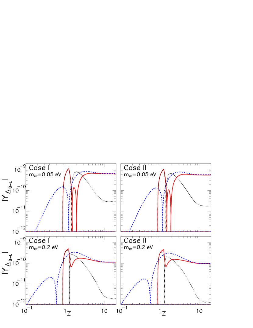
Figure II: Evolution of $Y_{\Delta_{B-L}}$. The solid continuous (red) line depict the complete results in the $m_{\widetilde{g}}=\mu_{\scriptscriptstyle\tilde{H}}\to 0\,$ limit. The dashed (blue) line correspond to the same limit but with all thermal corrections to the $CP$ asymmetries neglected. The dotted (black) line gives $Y_{\Delta_{B-L}}$ with thermal effects when SE is assumed. Panels on the left and right sides are respectively for Case I ($h_{e,d}$ Yukawa equilibrium) and Case II ($h_{e,d}$ Yukawa non-equilibrium). Upper and lower panels are respectively for $m_{\rm eff}=0.05\,$eV and $m_{\rm eff}=0.20\,$eV.

We plot in Figure II the evolution of $Y_{\Delta_{B-L}}$ with increasing $z=M/T$. The solid (red) lines correspond to the full results obtained in the $m_{\widetilde{g}},\,\mu_{\scriptscriptstyle\tilde{H}}\to 0\,$GeV limit, that is when particles-sparticles superequilibrating processes are completely switched off. The dashed (blue) lines give the results obtained in the same limit, but when all thermal corrections to the CP asymmetries are neglected, and $\epsilon_{s}=-\epsilon_{f}=\bar{\epsilon}/2$. From all the four panels we see that in the NSE regime neglecting thermal corrections is an excellent approximation that reproduces with very good accuracy the (sizable) final values of $Y_{\Delta_{B-L}}$. The dotted (black) lines give $Y_{\Delta_{B-L}}$ in the usual treatments which includes thermal corrections and also assumes SE, that in our treatment corresponds to taking the limit $m_{\widetilde{g}},\mu_{\scriptscriptstyle\tilde{H}}\to\infty$. Panels on the left side refer to Case I discussed in Section 4.3, panels on the right side are for Case II discussed in Section 4.4. We can see that the differences between the situations in which the $h_{e,d}$ Yukawa reactions are in equilibrium and when they are out of equilibrium are rather mild. Therefore in the following we will concentrate just on results for Case I. Upper and lower panels correspond instead to two different strength for the washout processes, parameterized respectively by $m_{\rm eff}=0.05\,$eV and $m_{\rm eff}=0.20\,$eV. As it was expected from the analysis in the previous section, we see that the stronger the washouts, the larger is the gain in efficiency with respect to the SE scenario.

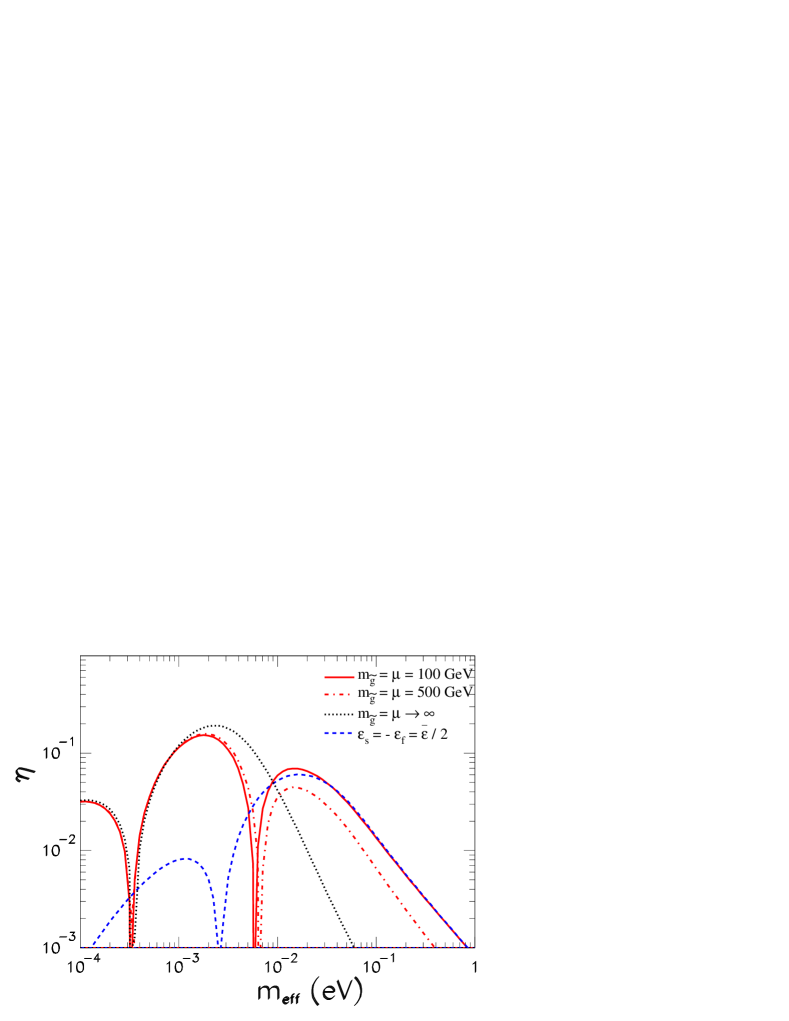
Figure III: Efficiency factor $\eta$ as a function of the washout parameter $m_{\rm eff}$ for Case I ($h_{e,d}$ Yukawa equilibrium) and different values of $m_{\widetilde{g}}=\mu_{\scriptscriptstyle\tilde{H}}$. The red continuous line corresponds to the $m_{\widetilde{g}}=\mu_{\scriptscriptstyle\tilde{H}}=100\,$ GeV which is still in the full NSE regime, while the dashed blue line to the same limit but with thermal corrections neglected. The red dash-dotted line corresponds respectively to $m_{\widetilde{g}}=\mu_{\scriptscriptstyle\tilde{H}}=500\,$GeV, and the black dotted line to SE with $m_{\widetilde{g}},\,\mu_{\scriptscriptstyle\tilde{H}}\to\infty$.

In Figure III we plot for Case I the efficiency $\eta$ defined in Eq. (80) as a function of the washout parameter $m_{\rm eff}$. The red continuous line corresponds to $m_{\widetilde{g}}=\mu_{\scriptscriptstyle\tilde{H}}=100\,$GeV. We have chosen a non-zero value for these parameters because of phenomenological motivations, however we have checked that the results are practically indistinguishable from those obtained in the $m_{\widetilde{g}}=\mu_{\scriptscriptstyle\tilde{H}}\to 0\,$ limit and thus, in agreement with Eq. (25), the evolution still occurs in the full NSE regime. The red dash-dotted line corresponds to $m_{\widetilde{g}}=\mu_{\scriptscriptstyle\tilde{H}}=500\,$ GeV. We can see that in this case SE rates start suppressing the efficiency, but are still far from attaining full thermal equilibrium. The black dotted line corresponds to the $m_{\widetilde{g}},\,\mu_{\scriptscriptstyle\tilde{H}}\to\infty\,$ limit of complete SE. We see that if SE is incorrectly assumed in temperature ranges where it does not occur, one could vastly underestimate the leptogenesis efficiency. The size of this underestimation is a fast increasing function of the washouts, and for particularly large values of $m_{\rm eff}$ can reach the two orders of magnitude level. Let us also note that for $m_{\rm eff}\ \hbox to0.0pt{\raise 3.0pt\hbox{$>$}\hss}{\lower 3.0pt\hbox{$\sim$}}\ 6\times 10^{-3}\,$eV, the assumption of SE results in a baryon asymmetry of the wrong sign. Graphically, one can see this from the fact that at small values of $m_{\rm eff}$ the black and red lines approximately overlap, and then both change sign around $m_{\rm eff}\sim 3\times 10^{-4}\,$eV. But around $m_{\rm eff}\sim 6\times 10^{-3}\,$eV for the red line there is another sign change. This marks the onset of $R$-genesis domination; therefore, from this point onward, baryogenesis does not proceed through leptogenesis, but rather through $R$-genesis.

In the same figure we have also plotted with the dash blue continuous line the NSE results in the approximation of neglecting all thermal corrections to the $CP$ asymmetries. By comparing with the full results (red continuous line) we see that for $m_{\rm eff}\ \hbox to0.0pt{\raise 3.0pt\hbox{$>$}\hss}{\lower 3.0pt\hbox{$\sim$}}\ {\rm few}\,\times 10^{-2}\,$eV thermal corrections give negligible effects. We conclude that in the case of $R$-genesis, the zero temperature approximation yields quite reliable results.

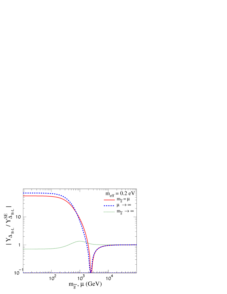
Figure IV: The final value of $Y_{\Delta_{B-L}}$ normalized to the SE result $Y^{SE}_{\Delta_{B-L}}$ as a function of $m_{\widetilde{g}}$ and $\mu_{\scriptscriptstyle\tilde{H}}$ for Case I ($h_{e,d}$ Yukawa equilibrium) and $m_{\rm eff}=0.20\,$eV. The red continuous line corresponds to varying simultaneously both parameters holding $m_{\widetilde{g}}=\mu_{\scriptscriptstyle\tilde{H}}$. The blue dashed line corresponds to varying only $m_{\widetilde{g}}$ in the limit $\mu_{\scriptscriptstyle\tilde{H}}\to\infty$. The green dotted line corresponds to varying only $\mu_{\scriptscriptstyle\tilde{H}}$ in the limit $m_{\widetilde{g}}\to\infty$.

In Figure IV we plot the final value of $Y_{\Delta_{B-L}}$ as a function of different values of $m_{\widetilde{g}}$ and $\mu_{\scriptscriptstyle\tilde{H}}$, normalized for convenience to the value $Y^{SE}_{\Delta_{B-L}}$ obtained when SE is assumed. The results correspond again to Case I discussed in Section 4.3. In order to enhance the impact of the new effects, we have fixed the washout parameter to a rather large value $m_{\rm eff}=0.20\,$eV. The red continuous line corresponds to varying simultaneously both SE parameters keeping their values equal: $m_{\widetilde{g}}=\mu_{\scriptscriptstyle\tilde{H}}$. We see that for $m_{\widetilde{g}}=\mu_{\scriptscriptstyle\tilde{H}}\ \hbox to0.0pt{\raise 3.0pt\hbox{$<$}\hss}{\lower 3.0pt\hbox{$\sim$}}\ 1\,$TeV the amount of $B-L$ asymmetry produced by soft leptogenesis can be up to two orders of magnitude larger (and of the opposite sign) with respect to what would be obtained in the usual approach with SE. SE effects start suppressing the asymmetry around $m_{\widetilde{g}}=\mu_{\scriptscriptstyle\tilde{H}}\sim 1\,$TeV. The asymmetry then changes sign around $3\,$TeV, that marks the transition from the $R$-genesis to the leptogenesis regime, and eventually around $5\,$TeV SE reactions attain complete thermal equilibrium and $Y_{\Delta_{B-L}}/Y^{SE}_{\Delta_{B-L}}\to 1$.

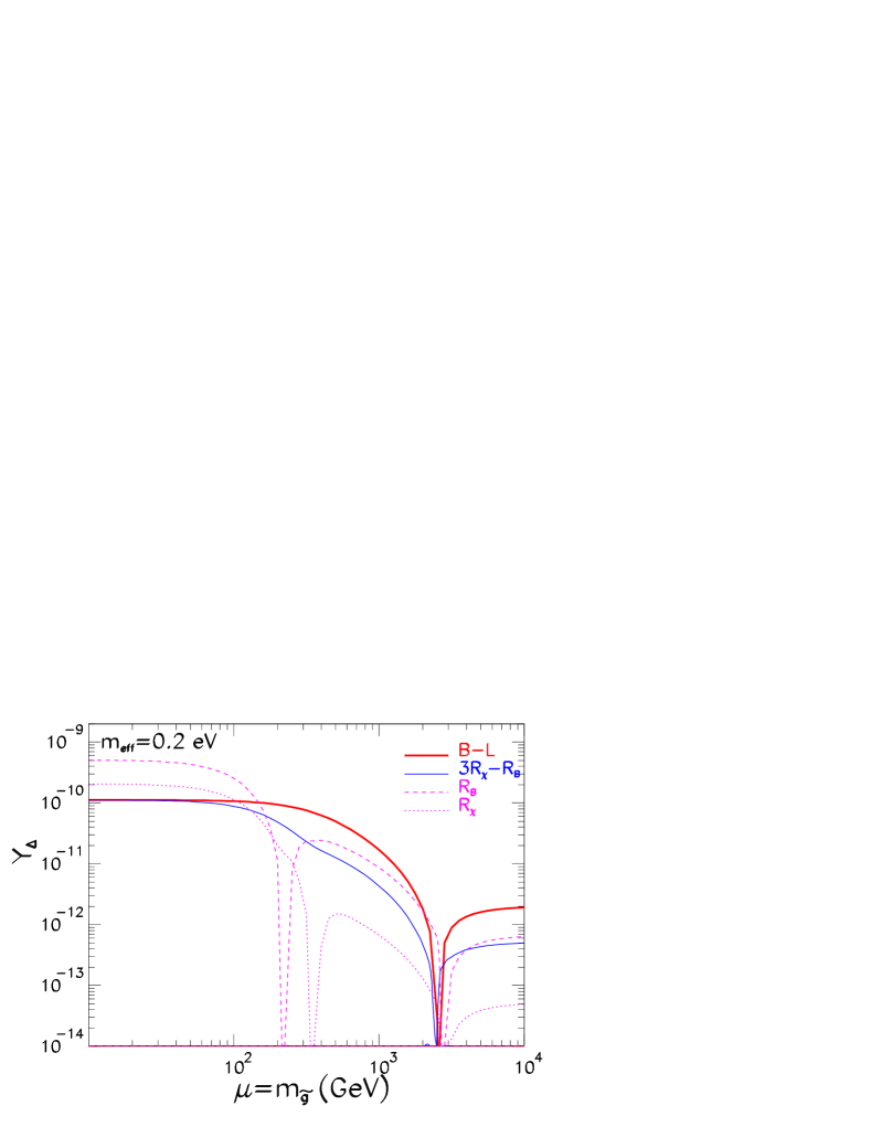
Figure V: Final values of the charge density asymmetries as a function of $m_{\widetilde{g}}=\mu_{\scriptscriptstyle\tilde{H}}$ for Case I ($h_{e,d}$ Yukawa equilibrium) and $m_{\rm eff}=0.20\,$eV. Thick red line: $Y_{\Delta_{B-L}}$; thick blue line: $3Y_{\Delta R_{\chi}}-Y_{\Delta R_{B}}$; thin dashed purple line: $Y_{\Delta{R_{B}}}$; thin dotted purple line: $Y_{\Delta{R_{\chi}}}$.

It can be of some interest knowing what happens if only one of the two anomalous symmetries $U(1)_{R}$ or $U(1)_{PQ}$ were present. While we have not constructed such theories, our BE equations are sufficiently general to allow exploring numerically also these cases. The corresponding results are also depicted in Figure IV. The blue dashed line corresponds to the $U(1)_{R}$-theory where $m_{\widetilde{g}}$ is varied while $U(1)_{PQ}$ is broken. The green dotted line corresponds to the alternative $U(1)_{PQ}$-theory in which $m_{\widetilde{g}}\to\infty$ and only $\mu_{\scriptscriptstyle\tilde{H}}$ is varied. From these results we see that the real responsible of the large effects is the $R$-symmetry, while the effects of the $PQ$ symmetry remains qualitatively more at the level of typical spectator effects. A theoretical justification of this behavior is not difficult to find, and we will discuss it in the following concluding section.

Some important aspects of the transition from $R$-genesis (NSE regime) to leptogenesis (SE regime) are highlighted in figure V, where we plot the final value of the relevant charge density-asymmetries as a function of $m_{\widetilde{g}}=\mu_{\scriptscriptstyle\tilde{H}}$, assuming Case I and $m_{\rm eff}=0.20\,$eV. The thick solid red line corresponds to $Y_{\Delta_{B-L}}$, while the thin solid blue line corresponds to $3Y_{\Delta R_{\chi}}-Y_{\Delta R_{B}}$. The thin dashed and dotted purple lines display respectively $Y_{\Delta{R_{B}}}$ and $Y_{\Delta{R_{\chi}}}$. We see that up to $m_{\widetilde{g}}=\mu_{\scriptscriptstyle\tilde{H}}\sim 100\,$GeV we have $Y_{\Delta_{B-L}}\simeq 3Y_{\Delta R_{\chi}}-Y_{\Delta R_{B}}$ that is in agreement with Eq. (74), and thus implies that baryogenesis occurs almost only via $R$-genesis. As the soft supersymmetry-breaking parameters are increased, SE reactions begin to wash out efficiently $Y_{\Delta{R_{B}}}$ and $Y_{\Delta{R_{\chi}}}$ but the difference $3Y_{\Delta{R_{\chi}}}-Y_{\Delta{R_{B}}}$ still remains of the order of $Y_{\Delta_{B-L}}$, and $R$-genesis still gives the dominant contribution to baryogenesis.

Around $m_{\widetilde{g}}=\mu_{\scriptscriptstyle\tilde{H}}\sim 3\,$TeV all the charge asymmetries change simultaneously their sign. This is the benchmark of the onset of the regime in which leptogenesis dominates. The only relevant source for generating the density-asymmetries is now the (opposite-sign) thermally induced $B-L$ asymmetry, that is not affected by SE washouts, and that is feeding (small) asymmetries into all the other charges. In this regime $Y_{\Delta_{R_{B}}}$ and $Y_{\Delta_{R_{\chi}}}$ do not have anymore an independent dynamics, and can be simply computed in terms of $Y_{\Delta_{B-L}}$ yielding $Y_{\Delta{R_{B}}}=-\frac{1}{3}Y_{\Delta_{B-L}}$ and $Y_{\Delta{R_{\chi}}}=-\frac{3}{79}\,Y_{\Delta_{B-L}}$.

7 Discussion and conclusions

The supersymmetric seesaw model unavoidably entails the possibility of soft leptogenesis. The interest in this possibility relies on the fact that while supersymmetric leptogenesis can only proceed within temperature regimes that are in strong tension with the bounds from overproduction of gravitinos, typical soft leptogenesis temperatures are sensibly lower, and can accordingly relax this tension. However, soft leptogenesis is plagued by the problem of a congenital low efficiency, that is related to the cancellation between the asymmetries produced in fermions and bosons carrying lepton number. As we have discussed in length, this cancellation becomes almost exact in the zero temperature limit. Eventually, finite temperature corrections, that break supersymmetry and spoil the cancellation between the scalar and fermion CP asymmetries, can rescue soft leptogenesis from a complete failure.

It should be stressed at this point that the fact that lepton number $L$ commutes with supersymmetric transformations, that is that scalar and fermionic members of a supermultiplet have the same lepton number, plays a crucial role in enforcing the aforementioned CP asymmetry cancellation.

In this paper we have pointed out that in the temperature regime quantified by Eq. (25), in which all reactions that depend on the soft gaugino masses do not occur, the early Universe effective theory includes a new $R$-symmetry. In soft leptogenesis, this $R$-symmetry is violated in the out of equilibrium interactions of neutrinos and sneutrinos. In particular, $R$-number CP asymmetries in heavy sneutrino decays can be defined, and constitute important quantities. In fact, given that $R$-symmetries do not commute with supersymmetry transformations, it is hardly surprising that no cancellation occurs between the $R$-number CP asymmetries for scalars and fermions. For this reason, a sizable density asymmetry for the $R$ charge can develop in the thermal bath, and this asymmetry turns out to be the main responsible for the generation of the baryon asymmetry.

To keep higgsinos sufficiently light, in supersymmetry one needs to assume $\mu_{\scriptscriptstyle\tilde{H}}\sim m_{\tilde{g}}$, and thus when the gaugino masses are set to zero, one must set $\mu_{\scriptscriptstyle\tilde{H}}\to 0$ as well. In this limit the effective theory acquires another quasi-conserved global symmetry, that is a $U(1)_{PQ}$ symmetry of the Peccei-Quinn type. $PQ$ is also violated in sneutrino interactions and thus it also has an associated CP asymmetry. However, since $U(1)_{PQ}$ is a bosonic symmetry that commutes with supersymmetry, the same cancellation between fermion/boson $CP$ asymmetries occurring for lepton number also occurs for $PQ$. Accordingly, $PQ$ does not play an equivalently important role in the generation of the baryon asymmetry.

In order to make more understandable the previous two remarks, let us start from the beginning, by listing the relevant global symmetries of the effective theory. For simplicity we concentrate on Case I ($h_{e,d}$ Yukawa equilibrium). Neglecting lepton flavour, that is irrelevant for the present discussion, these symmetries are: $L,\,R,\,PQ,\,B$ and $\raise 2.0pt\hbox{$\chi$}_{u^{c}_{L}}$. The first three $L,\,R,\,PQ$ are violated perturbatively in the interactions of the heavy sneutrinos, and all five symmetries are violated by non-perturbative sphaleron processes. In this paper, in carrying out our analysis, we have first identified the anomaly free combinations of the five charges, that are $B-L$, $R_{B}$ and $R_{\chi}$, and then we have written down the BE to describe their evolution. Here, we want to sketch a different procedure. We first write a set of evolution equations for the five anomalous charges, that have the form:

$$\dot{Y}_{\Delta_{\cal Q}}={\cal S}_{\Delta_{\cal Q}}+{\cal G}_{\Delta_{\cal Q}}+{\cal G}^{NP}_{\Delta_{\cal Q}}\,.$$ (81)

In this equation ${\cal S}$ represent the source term for $Y_{\Delta}$, ${\cal G}$ is the (s)neutrino-related washouts with all density-asymmetries and signs absorbed, and ${\cal G}^{NP}$ represents the non-perturbative EW and/or QCD sphaleron reactions that violate $\Delta_{\cal Q}$. The latter are reactions of type (i), that is fast processes, that eventually will be convenient to eliminate in favor of chemical equilibrium conditions. Now, given that $B$ and $\raise 2.0pt\hbox{$\chi$}_{u^{c}_{L}}$ are good symmetries at the perturbative level, they have no CP-violating source term and ${\cal S}_{\Delta_{B}},\,{\cal S}_{\Delta_{\chi}}=0$ (they also do not have perturbative washouts, and ${\cal G}_{\Delta_{B}}$ ${\cal G}_{\Delta_{\chi}}=0$ too). The only source terms thus are ${\cal S}_{\Delta_{L}},\,{\cal S}_{\Delta_{PQ}}$ and ${\cal S}_{\Delta_{R}}$. However, as we already know, in the $T\to 0$ limit, for ${\cal S}_{\Delta_{L}}$ we have a cancellation between the fermion and scalar contributions: ${\cal S}^{f}_{\Delta_{L}}+{\cal S}^{s}_{\Delta_{L}}\to 0$. This straightforwardly implies that ${\cal S}^{f}_{\Delta_{PQ}}+{\cal S}^{s}_{\Delta_{PQ}}\to 0$ too, since the sneutrino processes contributing to the CP asymmetry for $PQ$ are the same than for $L$: they are simply multiplied by the appropriate $PQ$ charge that is, however, the same for fermion and scalar final states. For the $R$ charge we have instead ${\cal S}_{\Delta_{R}}\propto R_{f}\cdot{\cal S}^{f}_{\Delta_{L}}+R_{s}\cdot{\cal S}^{s}_{\Delta_{L}}$, where $R_{f,s}$ are respectively the overall $R$-charges of the fermion and boson two particle final state, and thus satisfy $R_{s}=R_{f}+2$. We then straightforwardly obtain that in the $T\to 0$ limit the $R$-charge source term does not vanish, and is given by ${\cal S}_{\Delta_{R}}\to 2\,{\cal S}^{s}_{\Delta_{L}}$. Fast in-equilibrium sphaleron processes enforce equilibrium conditions between particle densities carrying $R$ charge, and those carrying a $B$ and $L$ numbers and, as a result, eventually baryon and lepton asymmetries roughly of the same order than the $R$ charge-asymmetry develop. Eventually, with the decreasing of the temperature, gaugino mass related reactions will start occurring with in-equilibrium rates erasing any asymmetry in the $R$ charge. It is important to notice that when the $R$-symmetry gets explicitly broken, generalized EW sphalerons reduce to the standard EW sphalerons and sphaleron induced multi-fermion operators decouple from gauginos, and reduce to their standard $B+L$ violating form. Since gaugino mass reactions as well as all other MSSM processes conserve $B-L$, the asymmetry initially generated through $R$-genesis will remain unaffected.

Now that we have identified where the large density asymmetries come from, we can complete our procedure by constructing suitable linear combinations of the five equations (81) for which the sphaleron terms ${\cal G}^{NP}$ cancel out. Since there are only two such terms, ${\cal G}^{NP}_{EW}$ and ${\cal G}^{NP}_{QCD}$, we can construct three linear combinations in which only processes of type (iii) enter. These are the BE equations for the three anomaly free charges that have been discussed at length in Section 4.1. The equilibrium conditions enforced by ${\cal G}^{NP}_{EW}$ and ${\cal G}^{NP}_{QCD}$ have to be imposed on the system, and to obtain the BE in closed form, the various density-asymmetries appearing in the washout terms ${\cal G}$ must be rotated into the densities of the anomaly free charges by means of the appropriate $A$ matrix.

In this paper, we have not formulated possible alternative effective theories in which for example only $\mu_{\scriptscriptstyle\tilde{H}}=0$ is set to zero, that would correspond to an $U(1)_{PQ}$-theory, or the alternative case of having just an $U(1)_{R}$-theory. However, we have written down a set of BE that are sufficiently general to allow exploring numerically the outcome of such scenarios. The corresponding results are resumed in Figure IV, and confirm the crucial role played by the $R$ symmetry. In contrast, the effects ascribable to the new $PQ$ symmetry arising in the $\mu_{\scriptscriptstyle\tilde{H}}\to 0$ limit, that as we have seen are not related with any new large CP violating source, remain of the typical size of spectator effects.

In conclusion, supersymmetry offers different ways to explain the cosmic matter-antimatter asymmetry. The asymmetry could be directly generated in baryon number since, although severely constrained, EW baryogenesis has not been ruled out yet. Alternatively, the asymmetry could be initially generated in lepton number, through supersymmetric leptogenesis [13] or through soft-leptogenesis if it occurs below $T\sim 10^{7}\,$GeV. The main finding of our paper is that there is also a third, previously unnoticed, possibility. That is that the asymmetry can be first generated in the new $R$ charge that appears in the effective theory for supersymmetry when the Universe temperature is above $T\sim 10^{7}\,$GeV, and then transferred to baryons via generalized EW sphalerons.

Appendix A Thermal factors

In terms of the dimensionless evolution parameter $z=M/T$ the thermal factors appearing in the expressions of the decay CP asymmetries Eqs. (10)-(13) read:

$$\Delta_{s,f}(z)=\frac{c^{s,f}(z)}{c^{s}(z)+c^{f}(z)},$$ (82)

where, in the approximation in which $\widetilde{N}_{\pm}$ decay at rest,

$$c^{f}(z) = (1-x_{\ell}-x_{\widetilde{H}_{u}})\lambda(1,x_{\ell},x_{\widetilde{H}_{u}})\left[1-f_{\ell}^{eq}\right]\left[1-f_{\widetilde{H}_{u}}^{eq}\right],$$ (83)

$$c^{s}(z) = \lambda(1,x_{H_{u}},x_{\widetilde{\ell}})\left[1+f_{H_{u}}^{eq}\right]\left[1+f_{\widetilde{\ell}}^{eq}\right],$$ (84)

with

$$x_{a}(z) = \frac{m_{a}(z)^{2}}{M^{2}}\,,$$ (85)

$$\lambda(1,x,y) = \sqrt{(1+x-y)^{2}-4x}\,.$$ (86)

The Bose-Einstein $(s)$ and Fermi-Dirac $(f)$ equilibrium distributions are:

$$f^{eq}_{s} = \frac{1}{e^{z\varepsilon_{\!s}}-1}\,,\qquad\qquad s=\tilde{\ell},H_{u}\,,$$ (87)

$$f^{eq}_{f} = \frac{1}{e^{z\varepsilon_{\!f}}+1},\qquad\qquad f=\ell,\widetilde{H}_{u}\,,$$ (88)

where

$$\varepsilon_{\ell,\widetilde{H}_{u}} = \frac{1}{2}(1+x_{\ell,\widetilde{H}_{u}}-x_{\widetilde{H}_{u},\ell}),$$ (89)

$$\varepsilon_{\widetilde{\ell},H_{u}} = \frac{1}{2}(1+x_{\widetilde{\ell},H_{u}}-x_{H_{u},\widetilde{\ell}}).$$ (90)

Finally, the thermal masses for the relevant scalar and fermion particle species are [15]:

$$x_{H_{u}}=2\,x_{\widetilde{H}_{u}} = \frac{1}{z^{2}}\left(\frac{3}{8}g_{2}^{2}+\frac{1}{8}g_{Y}^{2}+\frac{3}{4}\lambda_{t}^{2}\right)\;,$$ (91)

$$x_{\widetilde{\ell}}\ =\ 2\,x_{\ell} = \frac{1}{z^{2}}\left(\frac{3}{8}g_{2}^{2}+\frac{1}{8}g_{Y}^{2}\right)\;,$$ (92)

where $g_{2}$ and $g_{Y}$ are the $SU(2)$ and $U(1)$ gauge couplings, and $\lambda_{t}$ is the top Yukawa coupling, renormalized at the appropriate energy scale.

Appendix B Boltzmann Equations

In this Appendix we present the Boltzmann equations that must be used for numerical studies of soft leptogenesis when the heavy sneutrino masses satisfy the condition Eq. (1). We also include the SE reactions $\gamma^{\rm eff}_{\tilde{g}}$ and $\gamma^{\rm eff}_{\scriptstyle\mu_{\scriptscriptstyle\tilde{H}}}$ defined in Eq. (66), that extend the validity of our BE to all temperatures.

The Boltzmann equations which describe the evolution of RH neutrino and sneutrino densities are:

$$\dot{Y}_{N} \!=\! -\left(\frac{Y_{N}}{Y_{N}^{eq}}-1\right)\left(\gamma_{N}+4\gamma_{t}^{(0)}+4\gamma_{t}^{(1)}+4\gamma_{t}^{(2)}+2\gamma_{t}^{(3)}+4\gamma_{t}^{(4)}\right),\qquad\qquad\mbox{\hskip 34.14322pt \phantom{i}}$$ (93)

$$\dot{Y}_{\widetilde{N}} \!=\! -\left(\frac{Y_{\widetilde{N}}}{Y_{\widetilde{N}_{+}}^{eq}}-2\right)\left(\frac{\gamma_{\widetilde{N}}}{2}+3\gamma_{22}+2\gamma_{t}^{\left(5\right)}+2\gamma_{t}^{\left(6\right)}+2\gamma_{t}^{\left(7\right)}+\gamma_{t}^{\left(8\right)}+2\gamma_{t}^{\left(9\right)}\right),$$ (94)

where the time derivative is defined as $\dot{Y}=sHz\frac{dY}{dz}$, $s$ is the entropy density, and $H=H(z)$ is the Hubble parameter. We have defined $Y_{\widetilde{N}}\equiv Y_{\widetilde{N}_{+}}+Y_{\widetilde{N}_{-}}\,$, and the reaction rates $\gamma$ without a flavour index $\alpha$ are always understood to be summed over all flavours. For the evolution of the flavour charges $Y_{\Delta_{\alpha}}$ we have

$$\dot{Y}_{\Delta_{\alpha}} = -\left(E_{\alpha}+\widetilde{E}_{\alpha}\right),$$ (95)

where

$$E_{\alpha} = \epsilon_{f}^{\alpha}\left(z\right)\frac{\gamma_{\widetilde{N}}}{2}\left(\frac{Y_{\widetilde{N}}}{Y_{\widetilde{N}_{+}}^{eq}}-2\right)-\frac{\gamma_{\widetilde{N}}^{f,\alpha}}{2}\left({\cal Y}_{\Delta\ell_{\alpha}}+{\cal Y}_{\Delta\widetilde{H}_{u}}\right)-\frac{1}{4}\gamma_{N}^{\alpha}\left({\cal Y}_{\Delta\ell_{\alpha}}+{\cal Y}_{\Delta H_{u}}\right)$$ (96)

$$-\left(\gamma_{t}^{\left(3\right)\alpha}\frac{Y_{N}}{Y_{N}^{eq}}+2\gamma_{t}^{\left(4\right)\alpha}+2\gamma_{t}^{\left(6\right)\alpha}+2\gamma_{t}^{\left(7\right)\alpha}+\gamma_{t}^{\left(5\right)\alpha}\frac{Y_{\widetilde{N}}}{Y_{\widetilde{N}_{+}}^{eq}}\right){\cal Y}_{\Delta\ell_{\alpha}}$$

$$-\left(\gamma_{t}^{\left(3\right)\alpha}+\gamma_{t}^{\left(4\right)\alpha}+\gamma_{t}^{\left(4\right)\alpha}\frac{Y_{N}}{Y_{N}^{eq}}+\gamma_{t}^{\left(5\right)\alpha}+\gamma_{t}^{\left(6\right)\alpha}+\frac{1}{2}\gamma_{t}^{\left(7\right)\alpha}\frac{Y_{\widetilde{N}}}{Y_{\widetilde{N}_{+}}^{eq}}\right){\cal Y}_{\Delta H_{u}}$$

$$-\left(\gamma_{t}^{\left(5\right)k}+\gamma_{t}^{\left(7\right)k}+\frac{1}{2}\gamma_{t}^{\left(6\right)k}\frac{Y_{\widetilde{N}}}{Y_{\widetilde{N}_{+}}^{eq}}\right)\left(2{\cal Y}_{\Delta\widetilde{H}_{u}}-{\cal Y}_{\Delta H_{u}}\right)$$

$$+\gamma_{\tilde{g}}^{\rm eff}\left({\cal Y}_{\Delta\widetilde{\ell}_{\alpha}}-{\cal Y}_{\Delta\ell_{\alpha}}\right),$$

and

$$\widetilde{E}_{\alpha} = \epsilon_{s}^{\alpha}\left(z\right)\frac{\gamma_{\widetilde{N}}}{2}\left(\frac{Y_{\widetilde{N}}}{Y_{\widetilde{N}_{+}}^{eq}}-2\right)-\frac{\gamma_{\widetilde{N}}^{s,\alpha}}{2}\left({\cal Y}_{\Delta\widetilde{\ell}_{\alpha}}+{\cal Y}_{\Delta H_{u}}\right)-\frac{1}{4}\gamma_{N}^{\alpha}\left({\cal Y}_{\Delta\widetilde{\ell}_{\alpha}}+{\cal Y}_{\Delta\widetilde{H}_{u}}\right)$$ (97)

$$-\left(\frac{1}{2}\gamma_{22}^{\alpha}\frac{Y_{\widetilde{N}}}{Y_{\widetilde{N}_{+}}^{eq}}+2\gamma_{22}^{\alpha}\right)\left({\cal Y}_{\Delta\widetilde{\ell}_{\alpha}}+2{\cal Y}_{\Delta\widetilde{H}_{u}}-{\cal Y}_{\Delta H_{u}}\right)$$

$$-\left(2\gamma_{t}^{\left(0\right)\alpha}\frac{Y_{N}}{Y_{N}^{eq}}+2\gamma_{t}^{\left(1\right)\alpha}+2\gamma_{t}^{\left(2\right)\alpha}+\frac{1}{2}\gamma_{t}^{\left(8\right)\alpha}\frac{Y_{\widetilde{N}}}{Y_{\widetilde{N}_{+}}^{eq}}+2\gamma_{t}^{\left(9\right)k}\right){\cal Y}_{\Delta\widetilde{\ell}_{\alpha}}$$

$$-\left(\gamma_{t}^{\left(0\right)\alpha}+\gamma_{t}^{\left(1\right)\alpha}\frac{Y_{N}}{Y_{N}^{eq}}+\gamma_{t}^{\left(8\right)\alpha}+\gamma_{t}^{\left(9\right)\alpha}+\frac{1}{2}\gamma_{t}^{\left(9\right)\alpha}\frac{Y_{\widetilde{N}}}{Y_{\widetilde{N}_{+}}^{eq}}\right){\cal Y}_{\Delta H_{u}}$$

$$-\left(\gamma_{t}^{\left(0\right)\alpha}+\gamma_{t}^{\left(1\right)\alpha}+\gamma_{t}^{\left(2\right)\alpha}\frac{Y_{N}}{Y_{N}^{eq}}\right)\left(2{\cal Y}_{\Delta\widetilde{H}_{u}}-{\cal Y}_{\Delta H_{u}}\right)$$

$$-\gamma_{\tilde{g}}^{\rm eff}\left({\cal Y}_{\Delta\widetilde{\ell}_{\alpha}}-{\cal Y}_{\Delta\ell_{\alpha}}\right).$$

The ${\cal Y}_{\Delta}$ appearing in these equations are defined in Eq. (60), while the SE reaction rate $\gamma_{\tilde{g}}^{\rm eff}$ has been defined in Eq. (66). For the decay reaction densities we have:

$$\gamma_{\widetilde{N}}^{s,\alpha} = \gamma_{\widetilde{N}}^{f,\alpha}\left(1+\frac{A^{2}}{M^{2}}-\frac{AB}{M^{2}}\right),$$

$$\gamma_{\widetilde{N}}^{\alpha} \equiv \gamma_{\widetilde{N}}^{f,\alpha}+\gamma_{\widetilde{N}}^{s,\alpha},$$ (98)

where $A$ and $B$ are taken to be real. For values $M\sim 10^{8}\,$GeV the higher order terms in the soft parameters can be safely neglected.

The scattering processes considered are

$$\begin{array}[]{|l|l|l|}\hline\cr\rm Reaction&\Delta R_{B}&\Delta R_{3}\\ \hline\cr\gamma_{22}^{\alpha}\equiv\gamma\left(\widetilde{N}_{\pm}\widetilde{\ell}_{\alpha}\leftrightarrow\widetilde{Q}\widetilde{u}^{*}\right)=\gamma\left(\widetilde{N}_{\pm}\widetilde{Q}^{*}\leftrightarrow\widetilde{\ell}_{\alpha}^{*}\widetilde{u}^{*}\right)=\gamma\left(\widetilde{N}_{\pm}\widetilde{u}\leftrightarrow\widetilde{\ell}_{\alpha}^{*}\widetilde{Q}\right)&0&1\\ \gamma_{t}^{(0)\alpha}\equiv\gamma\left(N\widetilde{\ell}_{\alpha}\leftrightarrow Q\widetilde{u}^{*}\right)=\gamma\left(N\widetilde{\ell}_{\alpha}\leftrightarrow\widetilde{Q}\overline{u}\right)&-1&0\\ \gamma_{t}^{(1)\alpha}\equiv\gamma\left(N\overline{Q}\leftrightarrow\widetilde{\ell}_{\alpha}^{*}\widetilde{u}^{*}\right)=\gamma\left(Nu\leftrightarrow\widetilde{\ell}_{\alpha}^{*}\widetilde{Q}\right)&-1&0\\ \gamma_{t}^{(2)\alpha}\equiv\gamma\left(N\widetilde{u}\leftrightarrow\widetilde{\ell}_{\alpha}^{*}Q\right)=\gamma\left(N\widetilde{Q}^{*}\leftrightarrow\widetilde{\ell}_{\alpha}^{*}\overline{u}\right)&-1&0\\ \gamma_{t}^{(3)\alpha}\equiv\gamma\left(N\ell_{\alpha}\leftrightarrow Q\overline{u}\right)&-1&0\\ \gamma_{t}^{(4)\alpha}\equiv\gamma\left(Nu\leftrightarrow\overline{\ell_{\alpha}}Q\right)=\gamma\left(N\overline{Q}\leftrightarrow\overline{\ell_{\alpha}}\overline{u}\right)&-1&0\\ \gamma_{t}^{(5)\alpha}\equiv\gamma\left(\widetilde{N}_{\pm}\ell_{\alpha}\leftrightarrow Q\widetilde{u}^{*}\right)=\gamma\left(\widetilde{N}_{\pm}\ell_{\alpha}\leftrightarrow\widetilde{Q}\overline{u}\right)&0&1\\ \gamma_{t}^{(6)\alpha}\equiv\gamma\left(\widetilde{N}_{\pm}\widetilde{u}\leftrightarrow\overline{\ell_{\alpha}}Q\right)=\gamma\left(\widetilde{N}_{\pm}\widetilde{Q}^{*}\leftrightarrow\overline{\ell_{\alpha}}\overline{u}\right)&0&1\\ \gamma_{t}^{(7)\alpha}\equiv\gamma\left(\widetilde{N}_{\pm}\overline{Q}\leftrightarrow\overline{\ell_{\alpha}}\widetilde{u}^{*}\right)=\gamma\left(\widetilde{N}_{\pm}u\leftrightarrow\overline{\ell_{\alpha}}\widetilde{Q}\right)&0&1\\ \gamma_{t}^{(8)\alpha}\equiv\gamma\left(\widetilde{N}_{\pm}\widetilde{\ell}_{\alpha}^{*}\leftrightarrow\overline{Q}u\right)&2&1\\ \gamma_{t}^{(9)\alpha}\equiv\gamma\left(\widetilde{N}_{\pm}Q\leftrightarrow\widetilde{\ell}_{\alpha}u\right)=\gamma\left(\widetilde{N}_{\pm}\overline{u}\leftrightarrow\widetilde{\ell}_{\alpha}\overline{Q}\right)&2&1\\ \hline\cr\end{array}$$

where for convenience we have listed the corresponding changes of the R-charges in each process. The reduced cross sections for the processes listed above can be found in ref. [14].

The BE above do not include the CP asymmetries of top and stop scatterings. Strictly speaking, when scatterings are included, for consistency one should include also the corresponding CP asymmetries. However, in soft leptogenesis this cannot be done in a straightforward way because thermal factors for the scattering CP asymmetries constitute a new set of non trivial quantities. Fortunately, in the strong washout regime for leptogenesis, the effects of CP asymmetries in scattering have been found to be subdominant with respect to CP asymmetries in decays [46], and since in this paper we focus precisely on strong washouts, neglecting the scattering CP asymmetries is justified.

The BE for the evolution of $R_{B}$ and $R_{\chi}$, defined in Eqs. (30)-(31), are:

$$\dot{Y}_{\Delta_{R_{B}}} = \sum_{\alpha}\left(2\widetilde{F}_{\alpha}+F_{\alpha}\right)-\gamma^{\rm eff}_{\widetilde{g}}\,{\cal Y}_{\Delta\widetilde{g}},$$ (99)

$$\dot{Y}_{\Delta_{R_{\chi}}} = \frac{1}{3}\sum_{\alpha}\left(\widetilde{G}_{\alpha}-G_{\alpha}\right)-\frac{\gamma^{\rm eff}_{\widetilde{g}}}{3}\,{\cal Y}_{\Delta\widetilde{g}}+\frac{\gamma^{\rm eff}_{\scriptstyle\mu_{\scriptscriptstyle\tilde{H}}}}{3}\left({\cal Y}_{\Delta\widetilde{H}_{u}}+{\cal Y}_{\Delta\widetilde{H}_{d}}\right),$$ (100)

where again the SE rates $\gamma^{\rm eff}_{\widetilde{g}}$ and $\gamma^{\rm eff}_{\scriptstyle\mu_{\scriptscriptstyle\tilde{H}}}$ have been also included. $F_{\alpha}$ and $\widetilde{F}_{\alpha}$ are given by:

$$F_{\alpha} = -\frac{1}{4}\gamma_{N}^{\alpha}\left({\cal Y}_{\Delta\ell_{\alpha}}+{\cal Y}_{\Delta H_{u}}\right)$$ (101)

$$-\left(\gamma_{t}^{\left(3\right)\alpha}\frac{Y_{N}}{Y_{N}^{eq}}+2\gamma_{t}^{\left(4\right)\alpha}\right){\cal Y}_{\Delta\ell_{\alpha}}$$

$$-\left(\gamma_{t}^{\left(3\right)\alpha}+\gamma_{t}^{\left(4\right)\alpha}+\gamma_{t}^{\left(4\right)\alpha}\frac{Y_{N}}{Y_{N}^{eq}}\right){\cal Y}_{\Delta H_{u}},$$

and

$$\widetilde{F}_{\alpha} = \epsilon_{s}^{\alpha}\left(z\right)\frac{\gamma_{\widetilde{N}}}{2}\left(\frac{Y_{\widetilde{N}}}{Y_{\widetilde{N}_{+}}^{eq}}-2\right)-\frac{\gamma_{\widetilde{N}}^{s,\alpha}}{2}\left({\cal Y}_{\Delta\widetilde{\ell}_{\alpha}}+{\cal Y}_{\Delta H_{u}}\right)-\frac{1}{8}\gamma_{N}^{\alpha}\left({\cal Y}_{\Delta\widetilde{\ell}_{\alpha}}+{\cal Y}_{\Delta\widetilde{H}_{u}}\right)$$ (102)

$$-\left(\gamma_{t}^{\left(0\right)\alpha}\frac{Y_{N}}{Y_{N}^{eq}}+\gamma_{t}^{\left(1\right)\alpha}+\gamma_{t}^{\left(2\right)\alpha}+\frac{1}{2}\gamma_{t}^{\left(8\right)\alpha}\frac{Y_{\widetilde{N}}}{Y_{\widetilde{N}_{+}}^{eq}}+2\gamma_{t}^{\left(9\right)\alpha}\right){\cal Y}_{\Delta\widetilde{\ell}_{\alpha}}$$

$$-\left(\frac{1}{2}\gamma_{t}^{\left(0\right)\alpha}+\frac{1}{2}\gamma_{t}^{\left(1\right)\alpha}\frac{Y_{N}}{Y_{N}^{eq}}+\gamma_{t}^{\left(8\right)\alpha}+\gamma_{t}^{\left(9\right)\alpha}+\frac{1}{2}\gamma_{t}^{\left(9\right)\alpha}\frac{Y_{\widetilde{N}}}{Y_{\widetilde{N}_{+}}^{eq}}\right){\cal Y}_{\Delta H_{u}}$$

$$-\frac{1}{2}\left(\gamma_{t}^{\left(0\right)\alpha}+\gamma_{t}^{\left(1\right)\alpha}+\gamma_{t}^{\left(2\right)\alpha}\frac{Y_{N}}{Y_{N}^{eq}}\right)\left(2{\cal Y}_{\Delta\widetilde{H}_{u}}-{\cal Y}_{\Delta H_{u}}\right).$$

For $G_{\alpha}$ and $\widetilde{G}_{\alpha}$ we have:

$$G_{\alpha} = \epsilon_{f}^{\alpha}\left(z\right)\frac{\gamma_{\widetilde{N}}}{2}\left(\frac{Y_{\widetilde{N}}}{Y_{\widetilde{N}_{+}}^{eq}}-2\right)-\frac{\gamma_{\widetilde{N}}^{f,\alpha}}{2}\left({\cal Y}_{\Delta\ell_{\alpha}}+{\cal Y}_{\Delta\widetilde{H}_{u}}\right)$$ (103)

$$-\left(2\gamma_{t}^{\left(6\right)\alpha}+2\gamma_{t}^{\left(7\right)\alpha}+\gamma_{t}^{\left(5\right)\alpha}\frac{Y_{\widetilde{N}}}{Y_{\widetilde{N}_{+}}^{eq}}\right){\cal Y}_{\Delta\ell_{\alpha}}$$

$$-\left(\gamma_{t}^{\left(5\right)\alpha}+\gamma_{t}^{\left(6\right)\alpha}+\frac{1}{2}\gamma_{t}^{\left(7\right)\alpha}\frac{Y_{\widetilde{N}}}{Y_{\widetilde{N}_{+}}^{eq}}\right){\cal Y}_{\Delta H_{u}}$$

$$-\left(\gamma_{t}^{\left(5\right)\alpha}+\gamma_{t}^{\left(7\right)k}+\frac{1}{2}\gamma_{t}^{\left(6\right)\alpha}\frac{Y_{\widetilde{N}}}{Y_{\widetilde{N}_{+}}^{eq}}\right)\left(2{\cal Y}_{\Delta\widetilde{H}_{u}}-{\cal Y}_{\Delta H_{u}}\right),$$

and

$$\widetilde{G}_{\alpha} = \epsilon_{s}^{\alpha}\left(z\right)\frac{\gamma_{\widetilde{N}}}{2}\left(\frac{Y_{\widetilde{N}}}{Y_{\widetilde{N}_{+}}^{eq}}-2\right)-\frac{\gamma_{\widetilde{N}}^{s,\alpha}}{2}\left({\cal Y}_{\Delta\widetilde{\ell}_{\alpha}}+{\cal Y}_{\Delta H_{u}}\right)$$ (104)

$$+\left(\frac{1}{2}\gamma_{22}^{\alpha}\frac{Y_{\widetilde{N}}}{Y_{\widetilde{N}_{+}}^{eq}}+2\gamma_{22}^{\alpha}\right)\left({\cal Y}_{\Delta\widetilde{\ell}_{\alpha}}+2{\cal Y}_{\Delta\widetilde{H}_{u}}-{\cal Y}_{\Delta H_{u}}\right)$$

$$-\left(\frac{1}{2}\gamma_{t}^{\left(8\right)\alpha}\frac{Y_{\widetilde{N}}}{Y_{\widetilde{N}_{+}}^{eq}}+2\gamma_{t}^{\left(9\right)\alpha}\right){\cal Y}_{\Delta\widetilde{\ell}_{\alpha}}$$

$$-\left(\gamma_{t}^{\left(8\right)\alpha}+\gamma_{t}^{\left(9\right)\alpha}+\frac{1}{2}\gamma_{t}^{\left(9\right)\alpha}\frac{Y_{\widetilde{N}}}{Y_{\widetilde{N}_{+}}^{eq}}\right){\cal Y}_{\Delta H_{u}}.$$

As we have explained, with the inclusion of $\gamma^{\rm eff}_{\widetilde{g}}$ and $\gamma^{\rm eff}_{\scriptstyle\mu_{\scriptscriptstyle\tilde{H}}}$ our BE are valid at all temperatures. To verify this, we have compared the results obtained with the complete BE given above, with what is obtained by integrating the set of BE specific for the SE regime, that reduce to the equations for the neutrino and sneutrino abundances Eq. (93) and Eq. (94) plus the three equations for the flavour charges Eq. (95). Of course, one also has to use the $A^{\ell}$ matrices and $C^{\widetilde{H}_{u}}$ vectors appropriate for the SE limits of the two cases that we have been studying (recalling also that $A^{\widetilde{\ell}}=2A^{\ell}$ and $C^{H_{u}}=2C^{\widetilde{H}_{u}}$). For Case I of Section 4.3 we have:

$$A^{\ell}=\frac{1}{9\times 237}\left(\begin{array}[]{ccc}-221&16&16\\ 16&-221&16\\ 16&16&-221\end{array}\right), C^{\tilde{H}_{u}}=\frac{-4}{237}\left(1,\;1,\;1\right),$$ (108)

that, incidentally, coincides with the matrix given in [13] for the case of all Yukawa couplings in equilibrium. The matrix for Case II of Section 4.4 is given in [13], and is rewritten below for convenience:

$$A^{\ell}=\frac{1}{3\times 2148}\left(\begin{array}[]{ccc}-906&\ \,\,120&\ \,\,120\\ \ \,75&-688&\ \,28\\ \ \,75&\ \,28&-688\end{array}\right), C^{\tilde{H}_{u}}=\frac{-1}{2148}\left(37,\;52,\;52\right).$$ (112)

References

- [1] M. Fukujita and T. Yanagida, Baryogenesis Without Grand Unification Phys. Lett. B174 (1986) 45
- [2] For a comprehensive review see: S. Davidson, E. Nardi and Y. Nir, Leptogenesis, Phys. Rept. 466, (2008) 105; [arXiv:0802.2962].
- [3] M. A. Luty, Baryogenesis via leptogenesis, Phys. Rev. D45, 455-465 (1992).
- [4] L. Covi, E. Roulet, F. Vissani, CP violating decays in leptogenesis scenarios, Phys. Lett. B384, 169-174 (1996) [hep-ph/9605319].
- [5] W. Buchmuller, M. Plumacher, Baryon asymmetry and neutrino mixing, Phys. Lett. B389, 73-77 (1996) [hep-ph/9608308].
- [6] A. Abada, S. Davidson, A. Ibarra, F. X. Josse-Michaux, M. Losada and A. Riotto, Flavour matters in leptogenesis, JHEP 0609, 010 (2006) [hep-ph/0605281].
- [7] E. Nardi, Y. Nir, E. Roulet and J. Racker, The importance of flavor in leptogenesis, JHEP 0601, 164 (2006), [hep-ph/0601084].
- [8] R. Barbieri, P. Creminelli, A. Strumia and N. Tetradis, Baryogenesis through leptogenesis, Nucl. Phys. B 575 (2000) 61 [hep-ph/9911315].
- [9] T. Endoh, T. Morozumi and Z. h. Xiong, Prog. Theor. Phys. 111, 123 (2004) [hep-ph/0308276]; T. Fujihara, S. Kaneko, S. Kang, D. Kimura, T. Morozumi and M. Tanimoto, Phys. Rev. D 72, 016006 (2005) [hep-ph/0505076].
- [10] O. Vives, Flavoured leptogenesis: A successful thermal leptogenesis with N(1) mass below 10**8-GeV, Phys. Rev. D 73 (2006) 073006 [hep-ph/0512160].
- [11] E. Nardi, Y. Nir, J. Racker and E. Roulet, On Higgs and sphaleron effects during the leptogenesis era, JHEP 0601, 068 (2006) [hep-ph/0512052].
- [12] W. Buchmuller and M. Plumacher, Spectator processes and baryogenesis, Phys. Lett. B511, 74 (2001) [hep-ph/0104189].
- [13] C. S. Fong, M. C. Gonzalez-Garcia, E. Nardi and J. Racker, Supersymmetric Leptogenesis, JCAP 1012, 013 (2010) [arXiv/1009.0003].
- [14] M. Plumacher, Baryon asymmetry, neutrino mixing and supersymmetric SO(10) unification, Nucl. Phys. B 530, 207 (1998) [hep-ph/9704231].
- [15] G. F. Giudice, A. Notari, M. Raidal, A. Riotto and A. Strumia, Towards a complete theory of thermal leptogenesis in the SM and MSSM, Nucl. Phys. B 685 (2004) 89, [hep-ph/0310123].
- [16] L. E. Ibanez and F. Quevedo, Supersymmetry Protects The Primordial Baryon Asymmetry, Phys. Lett. B283, 261 (1992) [hep-ph/9204205].
- [17] L. Boubekeur, Leptogenesis at low scale, [hep-ph/0208003].
- [18] Y. Grossman, T. Kashti, Y. Nir and E. Roulet, Leptogenesis from supersymmetry breaking, Phys. Rev. Lett. 91 (2003) 251801 [hep-ph/0307081].
- [19] G. D’Ambrosio, G. F. Giudice and M. Raidal, Soft leptogenesis, Phys. Lett. B575, 75 (2003) [hep-ph/0308031].
- [20] D. Aristizabal Sierra, M. Losada and E. Nardi, Variations on leptogenesis, Phys. Lett. B 659, 328 (2008) [arXiv/0705.1489].
- [21] D. A. Sierra, L. A. Munoz and E. Nardi, Purely Flavored Leptogenesis, Phys. Rev. D 80, 016007 (2009) [arXiv/0904.3043]; Implications of an additional scale on leptogenesis, J. Phys. Conf. Ser. 171, 012078 (2009) [arXiv/0904.3052].
- [22] D. Aristizabal Sierra, M. Losada and E. Nardi, Lepton Flavor Equilibration and Leptogenesis, JCAP 0912, 015 (2009) [arXiv/0905.0662].
- [23] S. Antusch, S. Blanchet, M. Blennow and E. Fernandez-Martinez, JHEP 1001, 017 (2010) [arXiv/0910.5957].
- [24] W. Fischler, G. F. Giudice, R. G. Leigh and S. Paban, Constraints on the baryogenesis scale from neutrino masses, Phys. Lett. B258, 45-48 (1991).
- [25] S. Davidson and A. Ibarra, A lower bound on the right-handed neutrino mass from leptogenesis, Phys. Lett. B535 (2002) 25, [hep-ph/0202239].
- [26] W. Buchmuller, P. Di Bari and M. Plumacher, Cosmic microwave background, matter-antimatter asymmetry and neutrino masses, Nucl. Phys. B 643 (2002) 367 [hep-ph/0205349]. J. R. Ellis and M. Raidal, Leptogenesis and the violation of lepton number and CP at low energies, Nucl. Phys. B 643 (2002) 229 [hep-ph/0206174].
- [27] A. Abada, S. Davidson, F. X. Josse-Michaux, M. Losada and A. Riotto, Flavour issues in leptogenesis, JCAP 0604 (2006) 004 [hep-ph/0601083].
- [28] S. Blanchet and P. Di Bari, Flavor effects on leptogenesis predictions, JCAP 0703, 018 (2007) [hep-ph/0607330];
- [29] A. Pilaftsis and T. E. J. Underwood, Resonant leptogenesis, Nucl. Phys. B 692 (2004) 303 [hep-ph/0309342]; A. Pilaftsis and T. E. J. Underwood, Electroweak-scale resonant leptogenesis, Phys. Rev. D 72 (2005) 113001 [hep-ph/0506107]; A. Pilaftsis, Resonant tau leptogenesis with observable lepton number violation, Phys. Rev. Lett. 95, 081602 (2005) [hep-ph/0408103].
- [30] E. Ma, N. Sahu and U. Sarkar, Leptogenesis below the Davidson-Ibarra bound, J. Phys. G 32, L65 (2006) [hep-ph/0603043]; Y. Farzan and J. W. F. Valle, R-parity violation assisted thermal leptogenesis in the seesaw mechanism, Phys. Rev. Lett. 96, 011601 (2006) [hep-ph/0509280]; N. Okada and O. Seto, Thermal leptogenesis in brane world cosmology, Phys. Rev. D 73, 063505 (2006) [hep-ph/0507279].
- [31] J. A. Casas, J. R. Espinosa, I. Hidalgo, Implications for new physics from fine-tuning arguments. 1. Application to SUSY and seesaw cases, JHEP 0411, 057 (2004) [hep-ph/0410298].
- [32] M. Y. Khlopov and A. D. Linde, Is It Easy To Save The Gravitino?, Phys. Lett. B 138 (1984) 265; J. R. Ellis, J. E. Kim and D. V. Nanopoulos, Cosmological Gravitino Regeneration And Decay Phys. Lett. B145 (1984) 181; J. R. Ellis, D. V. Nanopoulos and S. Sarkar, The Cosmology Of Decaying Gravitinos Nucl. Phys. B 259 (1985) 175; T. Moroi, H. Murayama and M. Yamaguchi, Cosmological constraints on the light stable gravitino, Phys. Lett. B B303 (1993) 289; M. Kawasaki, K. Kohri and T. Moroi, Hadronic decay of late-decaying particles and big-bang nucleosynthesis, Phys. Lett. B 625 (2005) 7 [astro-ph/0402490].
- [33] C. S. Fong and M. C. Gonzalez-Garcia, Flavoured Soft Leptogenesis, JHEP 0806, 076 (2008) [arXiv/0804.4471].
- [34] C. S. Fong and M. C. Gonzalez-Garcia, On Quantum Effects in Soft Leptogenesis, JCAP 0808 (2008) 008 [arXiv/0806.3077].
- [35] J. Garayoa, M. C. Gonzalez-Garcia and N. Rius, Soft leptogenesis in the inverse seesaw model, JHEP 0702 (2007) 021 [hep-ph/0611311].
- [36] G. D’Ambrosio, T. Hambye, A. Hektor, M. Raidal and A. Rossi, Leptogenesis in the minimal supersymmetric triplet seesaw model, Phys. Lett. B 604 (2004) 199 [hep-ph/0407312]; M. C. Chen and K. T. Mahanthappa, Lepton flavor violating decays, soft leptogenesis and SUSY SO(10), Phys. Rev. D 70, 113013 (2004) [hep-ph/0409096]; Y. Grossman, R. Kitano and H. Murayama, Natural soft leptogenesis, JHEP 0506, 058 (2005) [hep-ph/0504160]; E. J. Chun and S. Scopel, Soft leptogenesis in Higgs triplet model, Phys. Lett. B 636, 278 (2006) [hep-ph/0510170]; A. D. Medina and C. E. M. Wagner, Soft leptogenesis in warped extra dimensions, JHEP 0612, 037 (2006) [hep-ph/0609052]; E. J. Chun and L. Velasco-Sevilla, SO(10) unified models and soft leptogenesis, JHEP 0708, 075 (2007) [hep-ph/0702039].
- [37] Y. Grossman, T. Kashti, Y. Nir and E. Roulet, New ways to soft leptogenesis, JHEP 0411 (2004) 080 [hep-ph/0407063].
- [38] C. S. Fong and M. C. Gonzalez-Garcia, On Gaugino Contributions to Soft Leptogenesis, JHEP 0903 (2009) 073 [arXiv/0901.0008].
- [39] S. Pascoli, S. T. Petcov and A. Riotto, Connecting low energy leptonic CP-violation to leptogenesis, Phys. Rev. D 75, 083511 (2007) [hep-ph/0609125]; G. C. Branco, R. Gonzalez Felipe and F. R. Joaquim, A new bridge between leptonic CP violation and leptogenesis, Phys. Lett. B 645 (2007) 432 [hep-ph/0609297]; S. Antusch and A. M. Teixeira, Towards constraints on the SUSY seesaw from flavour-dependent leptogenesis, JCAP 0702, 024 (2007) [hep-ph/0611232]; S. Pascoli, S. T. Petcov and A. Riotto, Leptogenesis and low energy CP violation in neutrino physics, Nucl. Phys. B 774, 1 (2007) [hep-ph/0611338]; G. Engelhard, Y. Grossman, E. Nardi and Y. Nir, The importance of leptogenesis, Phys. Rev. Lett. 99, 081802 (2007) [hep-ph/0612187].
- [40] V. Cirigliano, A. De Simone, G. Isidori, I. Masina and A. Riotto, Quantum Resonant Leptogenesis and Minimal Lepton Flavour Violation, JCAP 0801 (2008) 004 [arXiv/0711.0778].
- [41] A. De Simone and A. Riotto, On the impact of flavour oscillations in leptogenesis, JCAP 0702 (2007) 005 [hep-ph/0611357]; S. Blanchet, P. Di Bari and G. G. Raffelt, Quantum Zeno effect and the impact of flavour in leptogenesis, JCAP 0703, 012 (2007) [hep-ph/0611337].
- [42] C. S. Fong, M. C. Gonzalez-Garcia, E. Nardi and J. Racker, Flavoured soft leptogenesis and natural values of the B term, JHEP 1007, 001 (2010) [arXiv/1004.5125].
- [43] J. A. Harvey and M. S. Turner, Cosmological Baryon And Lepton Number In The Presence Of Electroweak Fermion Number Violation, Phys. Rev. D 42, 3344 (1990).
- [44] J. M. Cline, K. Kainulainen and K. A. Olive, On the erasure and regeneration of the primordial baryon asymmetry by sphalerons, Phys. Rev. Lett. 71, 2372 (1993) [hep-ph/9304321]; J. M. Cline, K. Kainulainen and K. A. Olive, Protecting the primordial baryon asymmetry from erasure by sphalerons, Phys. Rev. D 49, 6394 (1994) [hep-ph/9401208].
- [45] W. Y. Keung and L. Littenberg, Test Of Supersymmetry In E- E- Collision, Phys. Rev. D 28, 1067 (1983).
- [46] E. Nardi, J. Racker and E. Roulet, CP violation in scatterings, three body processes and the Boltzmann equations for leptogenesis, JHEP 0709, 090 (2007) [arXiv/0707.0378]; C. S. Fong, M. C. Gonzalez-Garcia and J. Racker, CP Violation from Scatterings with Gauge Bosons in Leptogenesis, [arXiv/1010.2209].