Effects of Magnetic Fields on Photoionised Pillars and Globules

Abstract

The effects of initially uniform magnetic fields on the formation and evolution of dense pillars and cometary globules at the boundaries of H II regions are investigated using 3D radiation-magnetohydrodynamics simulations. It is shown, in agreement with previous work, that a strong initial magnetic field is required to significantly alter the non-magnetised dynamics because the energy input from photoionisation is so large that it remains the dominant driver of the dynamics in most situations. Additionally it is found that for weak and medium field strengths an initially perpendicular field is swept into alignment with the pillar during its dynamical evolution, matching magnetic field observations of the ‘Pillars of Creation’ in M16 and also some cometary globules. A strong perpendicular magnetic field remains in its initial configuration and also confines the photoevaporation flow into a bar-shaped dense ionised ribbon which partially shields the ionisation front and would be readily observable in recombination lines. A simple analytic model is presented to explain the properties of this bright linear structure. These results show that magnetic field strengths in star-forming regions can in principle be significantly constrained by the morphology of structures which form at the borders of H II regions.

1 Introduction

The study of elephant trunks, pillars and globules, found at the borders of H II regions around massive stars, has received significant attention in recent years, both from an observational perspective and in theoretical and computational models. The famous ‘Pillars of Creation’ in M16 were observed at optical wavelengths with HST (Hester et al., 1996), in the IR (Indebetouw et al., 2007; Sugitani et al., 2007), and in sub-mm/radio (e.g. Pound, 1998; White et al., 1999), showing that these are dynamic structures with ongoing star formation which may or may not have been triggered by the radiation which has shaped the pillars. Smith et al. (2010b) provide strong evidence that pillars in the Carina Nebula are significant sites of sequential star formation propagating away from the older star clusters in this region, building on previous observations of synchronised star formation around the periphery of the nebula by Smith & Brooks (2007). On smaller scales, studies of T-Tauri star ages in the Orion Nebula (Lee et al., 2005; Lee & Chen, 2007) show decreasing stellar ages moving away from massive stars and towards bright-rimmed clouds at the H II region/molecular cloud interface, again strongly suggesting at least sequential and possibly triggered star formation. The clear relationship between pillars/globules and second generation star formation around OB associations, and the question of the extent to which this star formation is triggered, provides strong motivation to understand the formation and evolution of these structures.

In a previous paper (Mackey & Lim, 2010, hereafter ML10) we investigated the formation and evolution of dense pillars of gas and dust – elephant trunks – on the boundaries of H II regions using 3D hydrodynamical simulations including photoionising radiative transfer (R-HD). It was found that shadowing of ionising radiation by an inhomogeneous density field naturally forms elephant trunks without the assistance of self-gravity, or of ionisation front and cooling instabilities. A combination of radiation-driven implosion (RDI; Bertoldi, 1989) and acceleration due to the rocket effect (Oort & Spitzer, 1955) produce elongated structures: RDI compresses neutral gas until pressure equilibrium with ionised gas is achieved; the rocket effect accelerates gas away from the radiation source producing dynamic elongated structures with lifetimes of a few hundred kyr (depending on clump masses/densities). Strong neutral gas cooling was found to enhance this formation mechanism, producing denser and longer lived pillar-like structures compared to models with weak cooling.

Models such as these for the formation of bright-rimmed clouds, globules and pillars have been considered for many years (e.g. Pottasch, 1958; Marsh, 1970; Bodenheimer et al., 1979; Sandford et al., 1982); much of this work is summarised by Yorke (1986). The RDI of a photoionised clump and its subsequent acceleration and evolution was calculated analytically (Bertoldi, 1989; Bertoldi & McKee, 1990) and subsequently numerically by Lefloch & Lazareff (1994). Williams et al. (2001) considered a range of axisymmetric models showing that multiple scenarios could form long-lived pillar-like structures. It has been shown (Kessel-Deynet & Burkert, 2003; Miao et al., 2006; Pound et al., 2007; Bisbas et al., 2010) that RDI of single clumps can generate cometary globules and trigger gravitational collapse, but it is more difficult to form pillars like those in M16 because gas must accumulate to a high density in the shadowed tail region. Lim & Mellema (2003) showed how photoionisation of multiple clumps which partially shadow each other leads to dense gas accumulating in shadowed tail regions; it was suggested by Pound et al. (2007) that multiple clumps are required to quantitatively match observations of the pillars in M16. Recent models (Mellema et al., 2006b; Raga et al., 2009; Lora et al., 2009; Gritschneder et al., 2009, 2010, ML10) showed that elephant trunks can form quite naturally from the photoionisation of a clumpy density field under a range of initial conditions. Gritschneder et al. (2010) extended our previous work (ML10) which used static initial conditions by considering the photoionisation of dynamic density fields generated by isothermal decaying turbulence, measuring the formation of pillar-like structures as a function of turbulent Mach number.

Filamentary structure in an apparently helical geometry was found in the shadowed tail regions of a number of elephant trunks (Carlqvist et al., 1998, 2002, 2003), and it was suggested this could arise due to twisting of magnetic field lines. Velocity profiles for some trunks were shown to be consistent with solid-body rotation (Gahm et al., 2006), again consistent with a magnetic origin of the observed structure, although the actual magnetic field orientation and strength has not yet been measured for these structures. The magnetic field in cometary globules has been measured by optical polarimetry (Sridharan et al., 1996; Bhatt, 1999; Bhatt et al., 2004), showing in two cases a field orientation along the head–tail axis of the globule, but in one case (Bhatt, 1999) a perpendicular field was found. Sugitani et al. (2007) used near-IR polarimetry of background stars to measure the magnetic field in M16, finding an ordered large-scale field in the H II region, but within the pillars the field is aligned with the pillar axes and significantly misaligned with the ambient field by $\theta\sim 30$–$40^{\circ}$. They suggest this should constrain the magnetic field strength since it has not been strong enough to resist reorientation during the formation and evolution of the pillars, a suggestion we explore in more detail in this work.

Theoretical calculations of the effects of magnetic fields on the expansion of H II regions were first considered by Lasker (1966b). Using analytic calculations Redman et al. (1998) studied ionisation fronts with a plane-parallel magnetic field in the plane of the ionisation front. They found that the velocity separation between R-type and D-type solutions decreases with increasing field strength, and that D-critical ionisation fronts also advance into the neutral gas more rapidly for increasing field strength. In Williams et al. (2000) jump conditions for ionisation fronts with oblique magnetic fields were presented, together with 1D numerical models showing how an ionisation front could progress from fast-R-type through fast-D-type, slow-R-type, and finally to slow-D-type. These extra modes are allowed because fast and slow shocks detach from the ionisation front at different times and propagate into the neutral medium. This work was extended by Williams & Dyson (2001), who calculated the internal structures of stationary 1D ionisation fronts. They found that oblique fields could produce significant transverse velocities and regions where the transverse field component is significantly modified.

Williams (2007) used 2D slab-symmetric radiation-magnetohydrodynamics (R-MHD) simulations to study the photoevaporation flows from magnetised globules. In these models clumps with an initial density of $n_{\mathrm{H}}=2\times 10^{5}\,\mathrm{cm}^{-3}$ were placed in an ambient medium $10\times$ less dense. For simplicity a uniform magnetic field with various strengths and orientations was used. Plane-parallel radiation was assumed, with a thermal model where the temperature relaxed to a value between $100\,$K and $10\,000\,$K according to its ionisation fraction. It was found that for a weak field the ionised gas pressure dominates the dynamics and the field was swept into a configuration where it was parallel to the column of neutral gas behind the dense clump. For a sufficiently strong field, however, the field determined the dynamics and made the flow almost one-dimensional along field lines.

The first 3D R-MHD calculation including non-equilibrium photoionising radiative transfer was performed by Krumholz, Stone & Gardiner (2007). They used the Athena code with a new ray-tracing module to simulate the expansion of an H II region around a point source in a uniform magnetic field. The overall expansion is now axisymmetric rather than spherically symmetric (cf. Lasker, 1966a) with a dense shell forming in directions parallel to the field, and a possibly numerical instability developing for expansion perpendicular to the field.

Using similar methods, Henney et al. (2009) model the photoionisation of a dense clump of gas in 3D with an initially uniform magnetic field. They use the photon-conserving C²-ray ray-tracing algorithm (Mellema et al., 2006a) which allows large timesteps to be taken without loss of accuracy. They found that the evolution of a photoionised globule can be significantly altered by the presence of a strong field, and in some cases a recombining shell forms at the termination shock of the photoevaporation flow when it is confined by a transverse field. The implosion phase is strongly asymmetric since the clump compresses much more readily along field lines than across them. These authors introduce a detailed thermal model to model the dynamics as realistically as possible for conditions in the Orion Nebula, finding that X-ray heating keeps the neutral gas temperature at $T\gtrsim 50\,$K, but the cooling in neutral gas is somewhat stronger than that considered in ML10.

In this work we add magnetic fields of various strengths and orientations to some of the models considered in ML10 to study their effects on the dynamics of the dense neutral gas. The simulation code is described in §2: §2.1 describes the MHD dynamics algorithm; §2.2 reviews the microphysical processes included; §2.3 presents a brief comparison of results obtained with our code to the test problem described by Krumholz et al. (2007). The 3D simulations presented here are introduced in §3 and our results presented in §4. §4.1 shows the evolution of the projected gas density and magnetic field orientation; §4.2 shows the emission from ionised gas; §4.3 evaluates boundary effects in strong field simulations. A calculation explaining the presence of a bright ionised linear ridge/ribbon in the strong field simulations is presented in §5. These results are compared to observations of H II regions and their magnetic fields in §6, where we also discuss our work in the context of other recent computational research. Our conclusions are presented in §7, and some technical details and tests for the simulations are given in the appendices.

2 Numerical Methods

2.1 MHD algorithms and tests

These calculations are performed on a uniform finite-volume grid, with the hydrodynamics and ray-tracing/microphysics modules as previously described in ML10. The simulations presented here use the same code, but with an MHD module coupled to the ray-tracing. The integration scheme was described by Falle et al. (1998) and is second order accurate in time and space, using the symmetric van Albada slope limiter to ensure monotonicity near shocks (van Albada et al., 1982). To calculate the MHD fluxes a number of Riemann solvers were tried; we use the Roe solver in conserved variables described by Cargo & Gallice (1997) as it was the most robust for these calculations (with corrections to typos obtained by comparison with Stone et al. 2008). Magnetic field units are used in the code such that factors of $4\pi$ do not appear in the dynamical equations (see e.g. Falle et al., 1998); c.g.s. units can be obtained by scaling the field strength by $\sqrt{4\pi}$. To avoid confusion we will always quote field strength in c.g.s. units (usually micro-Gauss, $\mu$G) rather than the code units. We use notation such that the total energy per unit volume is $E=\frac{1}{2}\rho v^{2}+p_{g}/(\gamma-1)+p_{m}$, being the sum of the kinetic, internal (thermal), and magnetic energies. The gas pressure is $p_{g}$, magnetic pressure is $p_{m}=B^{2}/8\pi$, and the ideal gas adiabatic index $\gamma$ is set to $5/3$. Multidimensional calculations use the artificial diffusion prescription of Falle et al. (1998) to fix the ‘carbuncle problem’ and to prevent rarefaction shocks developing; typically a viscosity parameter $\eta_{v}=0.1$ is used.

The code uses cell-centred values for vector quantities; the divergence constraint in the magnetic field is addressed using the ‘mixed-GLM’ divergence cleaning method of Dedner et al. (2002). This algorithm introduces an extra scalar field which couples to $\mathbf{\nabla}\cdot\mathbf{B}$, advecting and diffusing divergence errors so that they do not build up near shocks or other discontinuities. While it does allow non-zero divergence of $\mathbf{B}$ (which can introduce small force errors), the method has some advantages. (1) It is fully conservative in all of the physical variables; only the evolution equation for the unphysical scalar field, $\psi$, contains a source term. (2) The total energy and magnetic field updates are calculated in the same algorithmic step, ensuring they are consistent. An energy correction is still required, but this can be calculated from the fluxes generated by divergence cleaning. This means the internal energy (as a fraction of the total energy) is treated quite accurately, making the code robust for a wide range of field strengths. (3) It involves relatively little computational and memory overhead.

A number of 1D and multidimensional adiabatic MHD code tests have been performed to validate the code and for comparison to other astrophysical MHD codes. Results from a number of these test problems are shown in Appendix A and can also be found in more detail at http://www.astro.uni-bonn.de/~jmackey/jmac/ together with HD and photoionisation test problems (some of which were presented in ML10).

Three modifications have been made to the mixed-GLM divergence cleaning method. (1) The parameter $c_{r}$ is set to $c_{r}=4\Delta x$ (where the grid cell diameter is $\Delta x$) instead of the recommended value of $c_{r}=0.18$ (see Dedner et al., 2002, eq. 45). A typo in their paper (A. Dedner, private communication) meant $c_{r}$ should have been defined as $c_{r}=\Delta x/0.18$, similar to the value used here. (2) The algorithm induces extra magnetic field transport across cell boundaries; the energy associated with this is accounted for by an extra term in the energy flux:

$$F[E]\rightarrow F[E]+F[B_{x}]B_{x,m}\;.$$ (1)

Here $F[X]$ represents the flux of conserved variable $X$ across a cell boundary, $B_{x}$ is the component of $\mathbf{B}$ normal to the cell boundary, and $B_{x,m}$ is the value of $B_{x}$ in the interface state calculated using the mixed-GLM algorithm (Dedner et al., 2002, eq. 42). This correction removed gas pressure dips which appeared ahead of oblique shocks in axisymmetric models of magnetised jets. (3) Motivated by numerical difficulties encountered for subsonic flow across boundaries in magnetically dominated media, the boundary condition for the scalar field $\psi$ in the mixed-GLM method is modified for zero-gradient boundaries. This is described in Appendix B showing the improvement obtained with the new boundary condition.

2.2 Coupling MHD to photoionisation

We briefly review the microphysics algorithm here; the reader is referred to ML10 for further details. The dynamics and microphysics are solved separately in turn by operator splitting: in a given timestep the adiabatic MHD equations are solved and updated first (with the ion fraction advected with the gas flow), and then the internal energy per unit mass ($e_{\mathrm{int}}$) and ion fraction of Hydrogen ($x$) are updated by an adaptive sub-stepping integration to a user-specified relative accuracy. In the absence of photoionisation this uses a 5th order Runge–Kutta integration. Ray-tracing uses the short characteristics method with the photon-conserving discretisation of the photoionisation rate given by Mellema et al. (2006a). When a cell is strongly photoionised explicit integration is very unstable and so the ‘constant electron density’ approximation of Schmidt-Voigt & Koeppen (1987) is used (see also Mellema et al. 2006a) to analytically integrate the ion fraction when $x>0.95$. The time-averaged fraction of photons which pass through the cell is calculated simultaneously to obtain the appropriate cell optical depth for calculating rays to more distant grid cells. The algorithm used in ML10 was designed to work in an identical way for R-MHD as for R-HD. As such, the non-dynamical test problems presented in ML10 produce identical results when run with a non-zero magnetic field.

We continue to use the on-the-spot approximation for diffuse radiation; this remains a potential limitation of our results which should be checked with future work. Recent calculations including diffuse radiation (Raga et al., 2009; Williams & Henney, 2009) have shown that its role in the dynamics of H II regions may not be as significant as was suggested by e.g. Ritzerveld (2005). We plan to test this in dynamical simulations using an algorithm such as that described by Kuiper et al. (2010); it should be possible to extend their method to treat ionising photons.

Radiative cooling processes are modelled using the C2 cooling function from ML10 – in photoionised gas the coolants considered are collisionally excited emission from Oxygen and Nitrogen (Osterbrock, 1989) and recombining Hydrogen (Hummer, 1994), and neutral gas cooling is assumed to follow Newton’s Law of exponential cooling with a cooling time $t_{c}=10\,$kyr. Photoionisation assumes a monochromatic ionising source with $5.0\,$eV of thermal energy added to the gas per ionisation. Collisional ionisation is calculated using the rate of Voronov (1997).

2.3 H II region expansion with a magnetic field

Krumholz et al. (2007, hereafter KSG07) added a photoionisation module to the Athena code to calculate the 3D R-MHD expansion of an H II region into a uniform medium with an initially uniform magnetic field. We have modelled this problem both in axisymmetry and in 3D to compare results from our code to those of KSG07. Our 3D model used a smaller domain of diameter $14\,$pc resolved by $160^{3}$ cells (12 per cent larger cell diameters than KSG07). The only other difference in our simulation was to add a low level of noise to the otherwise uniform initial density and gas pressure fields. An initial ambient temperature of $T=100\,$K was used rather than the $11\,$K used by KSG07 and we used the C2 cooling function described above, but tests showed this does not affect the results significantly.

Gas density and velocity field are shown for a slice through the $x$–$y$ plane at $t\simeq 1.58\,$Myr in Fig. 1. Comparison to fig. 18 of KSG07 shows that very similar results are found here, notably the dense shell which forms for expansion in the $\pm\hat{\mathbf{x}}$ directions and its absence in perpendicular directions. We also find the instabilities which were noted by KSG07 in the perpendicular direction; we suggest they are real (i.e. not numerical artefacts) and related to the R-HD ionisation front instabilities studied by previous authors (e.g. Garcia-Segura & Franco, 1996; Williams, 2002; Whalen & Norman, 2008) on the basis of tests which showed the instabilities are only present when neutral gas can cool strongly. The velocity arrows show that the magnetic field significantly alters the ionised gas dynamics: at late times the strong outflow along field lines transforms the ionisation front to a recombination front in the $\pm\hat{\mathbf{x}}$ directions. We plan to study these features in more detail in future work.

Figure 1: R-MHD model of 3D H II region expansion. Results are shown at $1.58\,$Myr for a slice through the symmetry axis of the 3D simulation. Coordinate axes show position in parsecs, and gas number density is shown on a logarithmic scale from $n_{\mathrm{H}}=1$–$10^{3}\,\mathrm{cm}^{-3}$ as indicated. Velocity vectors are also shown where vector size is linearly proportional to velocity, $v$. The maximum velocity is $v_{\mathrm{max}}=6.7\,\mathrm{km}\,\mathrm{s}^{-1}$ in this figure. A white contour marking ion fraction $x=0.5$ is also shown. The $14.2\,\mu$G magnetic field is initially horizontal (parallel to the symmetry axis).

3 3D R-MHD simulations

To focus specifically on the effects of magnetic fields on the photoionisation process, the dense clump configurations in models 17 and 18 from ML10 were used rather than the random clump distributions in models 1–16. The two clump configurations as well as the simulation domain and radiation source properties are described in Table 1. Configuration 1 is basically the same as model 17 in ML10; configuration 2 is changed slightly – the two front clumps are slightly larger and further apart, and an extra clump is added further from the source. The radiation source located at the origin has the same properties as before: an ionising photon luminosity $L_{\gamma}=2\times 10^{50}\,\mathrm{s}^{-1}$ with monochromatic photon energy $h\nu_{0}-13.6\,\mathrm{eV}=5.0\,$eV. The simulation domain used here is twice as large in every dimension as was used for models 17 and 18 in ML10; this is because boundary effects were found to be much more significant with strong magnetic fields (cf. Henney et al., 2009). The simulation domain contains $384\times 256^{2}$ cells, giving a physical resolution of $\Delta x\simeq 0.012\,$pc per cell. Results of 3D R-MHD simulations with various domain sizes are described in Appendix C and demonstrate that the domain used here is sufficient to prevent significant boundary effects for all but the strongest fields modelled.

Config.	Object	$x$	$y$	$z$	$\delta_{0}$	$r_{0}$	M
1,2	$X_{\mathrm{min}}$	1.5	-1.5	-1.5	n/a	n/a	n/a
1,2	$X_{\mathrm{max}}$	6.0	1.5	1.5	n/a	n/a	n/a
1,2	Source	0	0	0	n/a	n/a	n/a
1	Cl 1	2.30	0	0	500	0.09	28.4
1	Cl 2	2.75	0	0.12	500	0.09	28.4
1	Cl 3	3.20	0	-0.12	500	0.09	28.4
2	Cl 1	2.30	0	-0.174	250	0.12	33.7
2	Cl 2	2.30	0	0.174	250	0.12	33.7
2	Cl 3	2.73	0	0	500	0.09	28.4
2	Cl 4	4.20	0.12	0.12	400	0.12	53.9

Table 1: Source and clump properties in R-MHD simulations. Configuration 1 is model 17 from ML10 and configuration 2 is a modified version of model 18 with an extra clump added further from the source. The domain minimum/maximum coordinates are measured in parsecs relative to the source, which is at the centre of the $y$–$z$ domain. Clump overdensities, $\delta_{0}$, are relative to the background number density of $n_{\mathrm{H}}=200\,\mathrm{cm}^{-3}$; their Gaussian scale radii, $r_{0}$, are in parsecs and their total masses, $M$, in units of $\mathrm{M}_{\odot}$.

These models were run with zero-gradient boundary conditions, which perfectly model supersonic outflow and damp reflected waves in subsonic outflow. There is nothing to stop inflow, however, if that is what the solution tends towards, and some of the R-MHD simulations do develop strong inflows at later times. An alternative boundary condition was imposed in the 2D slab-symmetric R-MHD simulations of Williams (2007): when the velocity was outward the usual zero-gradient boundary was applied, but if the velocity changed sign then inflow was suppressed. This ‘only-outflow’ boundary condition was also tested in our simulations to study how significantly inflows affected the solution, and in particular its observable properties. This was initially tested using axisymmetric simulations with a magnetic field parallel to the radiation propagation vector; the results showed that for a weak or medium field up to $B\sim 50\,\mu$G the inflow made little difference. Its only effect was to confine the photoevaporation flow from the clump to a smaller volume by the inflow’s ram pressure. The higher mean density of ionised gas (and associated stronger recombination) had no discernible dynamical effect. With a strong field of $B\simeq 160\,\mu$G, however, the inflow could overrun the photoevaporation flow and the ionisation front, transforming it into a recombination front and hence strongly affect the solution. For this reason the strong field simulation R8 described below was run with both a zero-gradient (as R8) and an only-outflow (as R8a) boundary condition in the direction back towards the radiation source.

3.1 Description of simulations

The simulations are listed in Table 2. R1 and R11 are R-HD simulations of clump configurations 1 and 2 respectively, while the other simulations are R-MHD calculations of the same clump configurations with varying field strengths and orientations. The field strengths were approximately $B\simeq 18,\ 53,$ and $160\,\mu$G and are referred to as weak, medium, and strong respectively. R2–R10 are R-MHD simulations of configuration 1: R2–R4 are weak field models, R5–R7 have a medium field, and R8–R10 a strong field. R12–R15 are R-MHD simulations of configuration 2: R11–R14 have a weak field and R15 a medium field.

For the field orientation, ‘parallel’ denotes parallel to the radiation propagation vector along the centre of the simulation ($\mathbf{B}=B_{0}\hat{\mathbf{x}}$), and ‘perpendicular’ denotes a field in the $y$–$z$ plane. Field orientations were chosen to be either parallel or perpendicular, or oriented $80^{\circ}$ from the $x$-axis and $50^{\circ}$ from the $y$-axis in the $y$–$z$ plane. The simulations with the latter field configuration (R3, R4, R7, R10) produced very similar results to the perpendicular models (R2, R5, and R8) for configuration 1 so they were not run for as long as the other models and were not run at all for configuration 2.

Whether a field is weak or strong is largely determined by its dynamical importance, set by the plasma parameter $\beta\equiv 8\pi p_{g}/B^{2}$, the ratio of thermal to magnetic pressure. Since ionised gas in H II regions is largely isothermal, as is dense molecular gas, the thermal pressure is approximately proportional to density. Hence a field of $50\,\mu$G could be strong or weak depending on whether the gas is ionised or neutral, and on its density. The plasma parameter is shown in Table 3 for a range of gas pressures encountered in the photoionisation simulations: (1) the initial conditions have a constant pressure of $p_{g}=1.38\times 10^{-11}\,\mathrm{dyne}\,\mathrm{cm}^{-2}$ (or $p_{g}/k_{\mathrm{B}}=10^{5}\,\mathrm{cm}^{-3}\,\mathrm{K}$); (2) gas at the background density of $n_{\mathrm{H}}=200\,\mathrm{cm}^{-3}$ and the ionised gas temperature of $T\simeq 8\,000\,$K has $p_{g}=4.42\times 10^{-10}\,\mathrm{dyne}\,\mathrm{cm}^{-2}$, and (3) the peak pressure typically encountered in the simulations is $p_{g}\sim 10^{-8}\,\mathrm{dyne}\,\mathrm{cm}^{-2}$. For weak field simulations the gas pressure clearly dominates and for the strong field the situation is reversed; for the medium field case the initial conditions are magnetically dominated but, once ionised, the gas pressure is larger. Thus it is expected that the weak field results will largely follow the R-HD results, the strong field simulations should show very different behaviour, and the medium field models will lie somewhere in between. The gas pressures in these simulations are comparable to those estimated for the pillars and their environment in M16 (see the discussion in ML10), but it should be borne in mind that other massive star-forming regions can have significantly higher (or lower) gas pressures.

Model	Cl.	BCs	$B_{x}$	$B_{y}$	$B_{z}$	$t_{\mathrm{sim}}$
R1	1	1	0	0	0	800
R2	1	2	1.77	1.77	17.7	525
R3	1	1	3.1	13.4	11.2	300
R4	1	2	3.1	13.4	11.2	300
R5	1	1	0	0	53.2	800
R6	1	1	53.2	0	0	800
R7	1	1	9.23	40.1	33.7	450
R8	1	1	14.2	7.1	158.9	400
R8A	1	3	14.2	7.1	158.9	400
R9	1	1	159.5	7.1	10.6	800
R10	1	1	27.7	120.3	101.0	280
R11	2	3	0	0	0	700
R12	2	3	1.77	1.77	17.7	375
R13	2	3	1.77	17.7	1.77	700
R14	2	3	17.7	1.77	1.77	700
R15	2	3	5.3	5.3	53.2	525

Table 2: Clump and initial magnetic field configurations, boundary conditions applied, and final simulation times for the R-MHD simulations. The two clump configurations indicated in column 2 are described in Table 1. For the boundary conditions (BCs, column 3), 1 refers to zero-gradient, 2 refers to only-outflow, and 3 is a hybrid where all boundaries are zero-gradient except for the boundary facing the source which is only-outflow. Field strengths are given in units of $\mu$Gauss. Some models have slightly off-axis field orientations to prevent any potential grid-alignment numerical effects. The simulations were evolved to the time shown by $t_{\mathrm{sim}}$ (in kyr).

$|\mathbf{B}|$ ($\mu$G)	$p_{g}=1.38\times 10^{-11}$,	$4.42\times 10^{-10}$,	$10^{-8}$
18	1.1	34	800
53	0.12	4.0	89
160	0.014	0.43	10

Table 3: Plasma beta ($\beta\equiv 8\pi p_{g}/B^{2}$) values for gas pressures encountered in R-MHD simulations, with $\beta\ll 1$ indicating magnetically dominated regions. The field strengths quoted are the three initial field strengths applied in the simulations. Gas pressures ($\mathrm{dyne}\,\mathrm{cm}^{-2}$) are representative of the initial conditions (2nd column), ionised gas at the background density (3rd column), and the typical maximum pressure near the ionisation front (4th column).

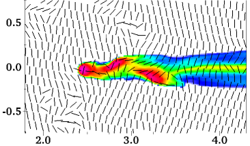
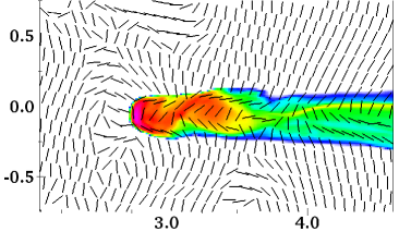
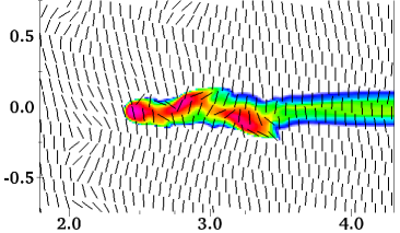
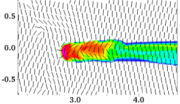
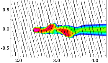
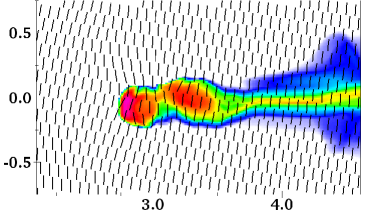
Figure 2: Projections along the $y$-axis for simulations R2 (top), R5 (centre), and R8 (bottom) at simulation times $100\,$kyr (left) and $200\,$kyr (right). Only part of the simulation domain is shown; positions are shown in parsecs relative to the source. Neutral gas column density is plotted on a logarithmic scale (cm^-2) as indicated. Projected magnetic field orientation (Eq. 2) is indicated by the black lines.

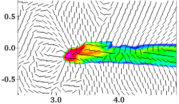
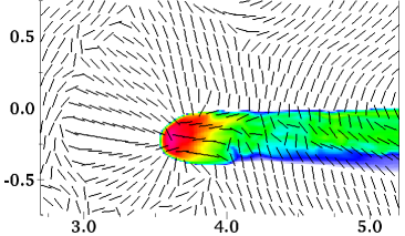
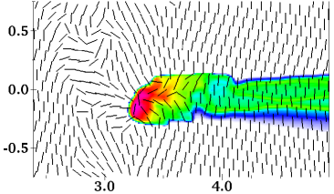
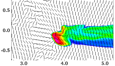
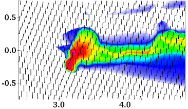
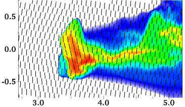
Figure 3: As Fig. 2, but for simulation times $300\,$kyr and $400\,$kyr.

4 Results

Three main observable consequences of the magnetic field are expected (Williams, 2007; Henney et al., 2009, cf.): (1) For weak magnetic fields the field orientation will be be changed by the dynamics of the photoionisation process. (2) When the field is sufficiently strong the density structure of the neutral gas will be significantly altered because gas can only move along field lines; RDI produces a sheet rather than an axisymmetric compression. (3) Strong magnetic fields will confine the photoevaporation flow changing its observable properties. We first plot projections through the simulation domain showing column density of neutral gas and the projected magnetic field. Following this we show emission maps in recombination radiation. R2, R5, and R8 proved most useful for showing the effects of increasing field strength so we focus most of our analysis on these three simulations.

4.1 Projected density and magnetic field

The column density is calculated as in ML10 by integrating the neutral gas number density along the line of sight (LOS). Note that because we do not consider molecules explicitly, the column densities should be divided by 2 to give N(H₂). The projected magnetic field is more difficult to calculate since it must be a weighted integral, for example to calculate the polarisation of background starlight induced by aligned dust grains (cf. observations of M16 by Sugitani et al., 2007). For our integration we assume a constant gas-to-dust ratio and weight the integral by gas density. To allow for the possibility that grain alignment may be less effective at high densities (e.g. Goodman et al., 1995) we limit the density weighting to a maximum density, $n_{\mathrm{max}}=2.5\times 10^{4}\,\mathrm{cm}^{-3}$; this is rather ad-hoc but it has a very limited effect on the projected field orientation as long as $n_{\mathrm{max}}\gtrsim 10^{4}\,\mathrm{cm}^{-3}$. The projected field may be calculated by integrating the Stokes $Q$ and $U$ parameters along the LOS and subsequently recovering the field orientation using trigonometric relations (see Arthur et al., 2010). With the approximations described above the projected $Q$ and $U$ parameters of the magnetic field are given by

$$\langle Q\rangle=\int_{s=0}^{\infty}\min[n_{\mathrm{H}}(s),n_{\mathrm{max}}]\frac{B_{1}^{2}-B_{2}^{2}}{\sqrt{B_{1}^{2}+B_{2}^{2}}}ds\,,$$

$$\langle U\rangle=\int_{s=0}^{\infty}\min[n_{\mathrm{H}}(s),n_{\mathrm{max}}]\frac{2B_{1}B_{2}}{\sqrt{B_{1}^{2}+B_{2}^{2}}}ds\,,$$ (2)

where $\hat{\mathbf{s}}$ is the LOS and the field perpendicular to the LOS is $\mathbf{B}_{p}=[B_{1},B_{2}]$. Technically this integration has units of $\mathrm{G}.\mathrm{cm}^{-2}$ but the normalisation was not considered because we only use the projected orientation of the field in this work and not its magnitude. In principle the relationship between polarisation and magnetic field is a very complex function of temperature, density, local radiation field and dust properties (e.g. Spitzer, 1998) but the microphysical processes included in our simulations are not sufficient to model this in any detail.

Results from the perpendicular field models R2, R5 and R8 are shown in Figs. 2 and 3 for simulation times 100, 200, 300 and $400\,$kyr. The LOS is the simulation $y$-axis so the initial field in all three simulations is almost vertical and perpendicular to the LOS. At $100\,$kyr the leading dense clump is just past the point of maximum compression due to RDI. The partially shadowed clumps are being compressed asymmetrically and are not yet at maximum compression. At this stage the structure of the dense gas is very similar in all three models, although it should be noted that the low density tail of the strong field model (R8) is actually a thin sheet seen edge-on, whereas it is closer to axisymmetric in R2. Already the magnetic field has been significantly altered in R2 due to RDI; this is less apparent in R5 while the field in R8 is almost unaffected. By $200\,$kyr the clumps have re-expanded somewhat (limited because much of the compressional heating was radiated away) but the rocket affect has taken hold and the first clump has almost fully merged with the second. At this stage the magnetic field re-orientation in R2 is more pronounced and in R5 is beginning to become significant. There are also differences in the morphology between the three models, quite slight between R2 and R5 but significant for R8. After $300\,$kyr the differences have become even more pronounced although the three clumps have basically merged to one in all three simulations. By $400\,$kyr R2 and R5 have become cometary globules rather than pillar-like structures. R5 is also fragmenting – the small protrusion at the top of the dense region eventually detaches from the main clump and is rapidly accelerated. R8 at this stage looks completely different to the other models. Low density gas has recombined behind the very broad ionisation front formed by gas expansion along the field lines. The field remains almost unchanged from its initial value even at this late stage.

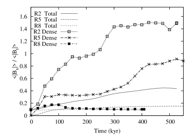
Figure 4: Evolution of the ratio of the mean parallel field $\langle|B_{x}|\rangle$ (volume averaged) to the mean perpendicular field $\langle\sqrt{B_{y}^{2}+B_{z}^{2}}\rangle$ for simulations R2, R5, R8.

The field evolution is shown in a more quantitative way in Fig. 4, where the ratio of the mean (volume averaged) parallel field $\langle|B_{x}|\rangle$ to perpendicular field $\langle\sqrt{B_{y}^{2}+B_{z}^{2}}\rangle$ is plotted as a function of time for both the full simulation domain and for only those cells with gas density $n_{\mathrm{H}}\geq 5\,000\,\mathrm{cm}^{-3}$. This ratio changes relatively little in the full domain because ionised gas takes up the overwhelming majority of the simulation volume. For the dense gas, however, a very strong effect is seen in the evolution as the field strength increases. The weak field in model R2 is swept into alignment with the pillar by the dynamics of RDI and the rocket effect, but a sufficiently strong field (here $\simeq 160\,\mu$G in R8) is unaffected.

In the parallel field models R6 and R9 there was very little field evolution because the rocket effect acts in the same direction as the initial field orientation. The results obtained are comparable to the S00L model in Henney et al. (2009), except that for R9 a strong inflow from the boundary closest to the source overran the ionisation front after $t\sim 200\,$kyr, leading to a stable 1D recombination front. This would not be expected to form if an only-outflow boundary is imposed, as in Williams (2007), although we note that for 1D photoionisation where ionised gas is confined to stay in the LOS back towards the source, a recombination front is a more stable and natural solution than an ionisation front.

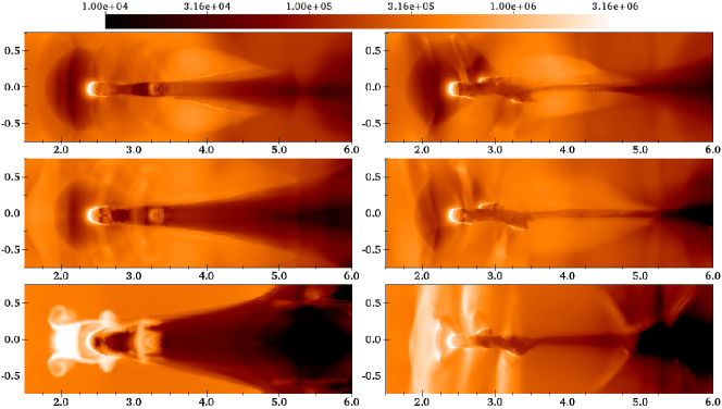
Figure 5: Projected recombination radiation maps of simulations R2 (top), R5 (centre) and R8 (bottom) for projections along the $z$-axis (left) and $y$-axis (right), here at $t=100\,$kyr. The initial field is along the $z$-axis for all three simulations. Energy flux on the indicated logarithmic scale has an arbitrary normalisation.

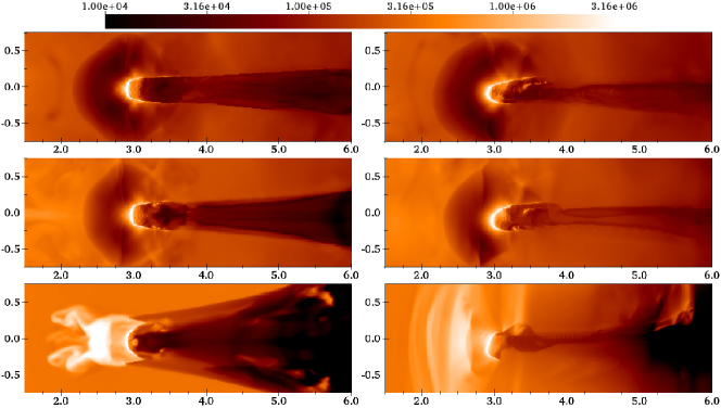
Figure 6: As Fig. 5 but at $t=250\,$kyr.

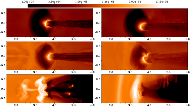
Figure 7: As Fig. 5 but at $t=400\,$kyr.

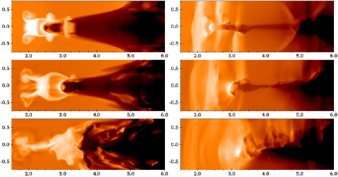
Figure 8: Similar to Fig. 5, but showing simulation R8a at $t=100\,$kyr (top), $t=250\,$kyr (middle) and $t=400\,$kyr (bottom). The left-hand plots show projection along the $z$-axis and the right-hand plots along the $y$-axis. These can be compared to R2, R5, and R8 in Figs. 5, 6 and 7.

4.2 Emission maps in recombination lines

The gas emission in recombination radiation (e.g. $\mathrm{H}\alpha$) was also calculated from the simulation outputs as in ML10, using the emissivity formula from Henney et al. (2005) and dust opacity as in Mellema et al. (2006b) to attenuate radiation along a LOS. Emission maps are shown at times 100, 250, and $400\,$kyr for models R2, R5, and R8 in Figs. 5, 6 and 7. Here, as in the column density maps, there are small differences between R2 and R5, but R8 shows very different emission. This can be understood from Table 3 which shows that only R8 is magnetically dominated in ionised gas. The initial field is along the LOS for the left-hand projections (LOS is simulation $z$-axis) and vertical for the right-hand projections (LOS is simulation $y$-axis).

The field is so weak in R2 that the evolution is very similar to the purely hydrodynamical evolution in R1 (cf. ML10) except that the low density shadowed tail region is not quite axisymmetric. A strong photoevaporation flow from the front clump expands spherically with velocity $v\simeq 30$–$35\,\mathrm{km}\,\mathrm{s}^{-1}$ until the ram pressure equals the total pressure of the ambient medium at which point a standing shock is established. For the full evolution of this model the dense gas at the ionisation front is by far the brightest structure in recombination emission. There are small differences in model R5, notably that the photoevaporation flow is confined to a smaller volume by the higher ambient total pressure, but the evolution is largely the same.

In R8 the total pressure of the ambient medium is magnetically dominated and much higher than in R2 or R5. This confines the photoevaporation flow much more effectively so that the region of spherical expansion is significantly smaller. Instead shocked photoionised gas is diverted along field lines into a bar-shaped linear structure with a density $2.5$–$4\times$ the background density. In Henney et al. (2009) this structure is termed a dense ribbon to avoid confusion with photon-dominated regions such as the Orion Bar (see e.g. O’Dell, 2001). We will avoid the term ‘bar’ for the same reason, instead referring to the structure as a ribbon or ridge (cf. Bohigas et al., 2004). This dense ionised gas is quite spatially extended and so has a comparable recombination radiation intensity to the bright rim at the ionisation front. Because of the high column density in the ribbon there is significant recombination in its shadow at later times. This evolution is similar to that seen in the strong field models of Henney et al. (2009).

The left-hand plots for R8 (with $\mathbf{B}$ along the LOS) show wave-like features which appear to be partially developed Kelvin–Helmholz instabilities. These move back towards the midplane ($y=0$) due to magnetic tension and have collided by $t=400\,$kyr (Fig. 7); similar but more pronounced evolution was found by Henney et al. (2009) in their simulations.

In simulation R8 at 400 kyr the dense ridge/ribbon has become optically thick, enhancing recombination in its shadow and dramatically weakening the photoevaporation flow. The result of this is that the standoff distance between the ridge and the original ionisation front of the dense clump has decreased almost to zero. This was found to be a short-lived phase in the models of Henney et al. (2009) and we expect the same to be true here because a strong photoevaporation flow is required to generate the overdense ionised gas.

4.3 Boundary effects for simulation R8

It was found that a reasonably strong inflow of gas developed at the boundary $x=1.5\,$pc in R8 at late times, ranging from $v_{x}=1$–$3.5\,\mathrm{km}\,\mathrm{s}^{-1}$. The ram pressure from this inflow could raise the density in the shocked region and hence affect the resulting evolution, so the simulation was repeated with this boundary set to only-outflow, thereby preventing the inflow developing. This simulation, denoted R8a, is shown in Fig. 8 at times 100, 250 and $400\,$kyr, again in recombination line emission. Comparison to Figs. 5 and 6 shows that the evolution is almost identical up to $t=250\,$kyr except that the bright ridge is slightly further from the ionisation front because now there is no ram pressure confinement. At $t=400\,$kyr the differences are more significant (see Fig. 7): the ionised ridge is broader and less well-defined in R8a than in R8, and while the dense neutral gas has a similar structure there are small differences. The general features remain the same, however, and the confined photoevaporation flow still shields the ionisation front significantly and outshines it in recombination radiation.

A similar but weaker inflow was also found in simulation R5. The only effect this has on the results is that the ionised ambient medium is denser than in R2, as seen by comparing the mean emission between the two simulations in Figs. 5–7.

5 Ionised Ridge formation

The presence of a bright ionised ridge/ribbon of dense gas in simulation R8 which is absent in R1, R2, and R5 is easily understood quantitatively by evaluating the jump conditions for the isothermal termination/reverse shock of the photoevaporation flow (the temperature is always in the range $7500$–$8500\,$K in the ionised gas). If we assume the system has reached an equilibrium, then the total pressure in the upstream (I), shocked (II), and downstream (III) regions will be equal. To avoid dealing with the spherical expansion of the photoevaporation flow we consider region I to consist only of the conditions immediately upstream from the shock (referred to below with subscript ‘1’). If we further assume that the only significant magnetic field is transverse to the velocity of expansion we can consider only its pressure effects and define a speed $b^{2}\equiv B^{2}/(8\pi\rho)=p_{m}/\rho$ so that the total pressure in a region is

$$P_{\mathrm{tot}}=p_{\mathrm{ram}}+p_{g}+p_{m}=\rho(v^{2}+c^{2}+b^{2})\,$$ (3)

being the sum of the ram, thermal and magnetic pressures respectively.

We wish to calculate the density in region II as a function only of the upstream velocity $v_{1}$ and the ambient medium properties ($b_{3}$, $v_{3}$). Only when the ratio $\rho_{2}/\rho_{3}>1$ will a bright ribbon or ridge be observable. Thus the equations to be solved are (cf. de Hoffmann & Teller, 1950)

$$k_{1}(v_{1}^{2}+c^{2}+b_{1}^{2})=k_{2}(v_{2}^{2}+c^{2}+b_{2}^{2})=(v_{3}^{2}+c^{2}+b_{3}^{2})\;,$$ (4)

where $k_{1}\equiv\rho_{1}/\rho_{3}$ and $k_{2}\equiv\rho_{2}/\rho_{3}$. The isothermal sound speed is $c^{2}\equiv p_{g}/\rho=kT/(\mu m_{p})$, where $\mu$ is the mean mass per particle in units of the proton mass $m_{p}$ and is $\mu=0.5$ in ionised gas in our models. For $T\simeq 8300\,$K this gives $c=11.7\,\mathrm{km}\,\mathrm{s}^{-1}$. In all simulations the magnetic field is negligible in region I ($b_{1}\ll c$) and smaller than the other terms in region II ($b_{2}<c$). The flow velocity in the reverse shock reference frame is $v_{1}\simeq 33$–$35\,\mathrm{km}\,\mathrm{s}^{-1}$ in all simulations giving a Mach number $M\equiv v_{1}/c\simeq 3$.

The hydrodynamic jump conditions for the isothermal reverse shock are

$$\frac{\rho_{2}}{\rho_{1}}=\frac{v_{1}^{2}}{c^{2}}=M^{2}\;,\qquad v_{2}=c/M\;.$$ (5)

When $b_{1}\simeq 0$ but $b_{2}>0$ the density jump is given by the solution to the quadratic equation

$$\left(\frac{\rho_{2}}{\rho_{1}}\right)^{2}-\left(\frac{\rho_{2}}{\rho_{1}}\right)\frac{v_{1}^{2}+c^{2}}{c^{2}+b_{2}^{2}}+\frac{v_{1}^{2}}{c^{2}+b_{2}^{2}}=0\;.$$ (6)

This equation has real solutions only for some values of $b_{2}$, leading to the constraint

$$0\leq\frac{b_{2}^{2}}{c^{2}}\leq\frac{M^{2}}{4}\left(1-\frac{1}{M^{2}}\right)^{2}\;.$$ (7)

For $M=3$ this gives $b_{2}^{2}\leq 16c^{2}/9$ but in the simulations it is actually significantly less than this limiting value.

Using these equations it is easy to show that in the hydrodynamic limit $k_{2}=M^{2}/(1+M^{2})\simeq 0.9$ and $k_{1}=1/(1+M^{2})\simeq 10$. No bright overdensity is formed, and the photoevaporation flow shocks at a density about $10\times$ below the ambient density. This is indeed seen in the R-HD simulation R1 and also the weak perpendicular field simulation R2.

With $b_{1}=v_{3}=0$ and $b_{3},b_{2}>0$ we obtain

$$k_{2}=\frac{b_{3}^{2}+c^{2}}{(c/M)^{2}+c^{2}+b_{2}^{2}} \geq\frac{1+(b_{3}/c)^{2}}{\left(\frac{1}{M}\right)^{2}+1+\frac{M^{2}}{4}\left(1-\frac{1}{M^{2}}\right)^{2}}\,,$$

$$k_{2} \leq\frac{M^{2}}{1+M^{2}}\left(1+\frac{b_{3}^{2}}{c^{2}}\right)$$ (8)

where the inequalities come from the limiting values for $b_{2}$ given by Eq. 7. With $M=3$ this gives

$$\frac{9}{26}\left(1+\frac{1}{\beta_{3}}\right)\leq k_{2}\leq\frac{9}{10}\left(1+\frac{1}{\beta_{3}}\right)$$ (9)

where $\beta_{3}\equiv p_{g}/p_{m}=c^{2}/b_{3}^{2}$. The overdensity in the post-shock region is therefore determined by the value of $(1+1/\beta)$ in the ionised ambient medium, showing that the ambient medium must be magnetically dominated to give an over-dense ridge. For R5 $\beta_{3}=4.0$ and for R8 $\beta_{3}=0.43$, leading to maximum overdensities $k_{2}$ of 1.1 and 3.0 respectively. Actual post-shock densities in R5 correspond very well to this value, and in R8/R8a the ribbon density is $n_{\mathrm{H}}\simeq 550$–$700\,\mathrm{cm}^{-3}$ depending on the time. The ambient density is $n_{\mathrm{H}}=200\,\mathrm{cm}^{-3}$ so the overdensity of $k_{2}=2.5$–$3.5$ is again close to the predicted value.

Similarly it is easy to show that $k_{1}=(1+1/\beta_{3})/(1+M^{2})$ giving $k_{1}=0.125$ and $0.33$ for R5 and R8. According to this equation the photoevaporation flow should shock for simulations R1, R2, R5 and R8 at $n_{\mathrm{H}}=20,\ 21,\ 25,\ 67\,\mathrm{cm}^{-3}$ respectively. In the simulations at $t=150\,$kyr the actual densities are $n_{\mathrm{H}}\simeq 25,\ 22,\ 31,\ 75\,\mathrm{cm}^{-3}$, whereas at $t=200\,$kyr they are $n_{\mathrm{H}}\simeq 18,\ 19,\ 30,\ 100\,\mathrm{cm}^{-3}$, in both cases comparable to the values predicted.

This simple model has obvious limitations, in particular we have not specified the form of the boundary between regions II and III – it is not a shock, but if the magnetic field strength changes significantly then a contact discontinuity forms to equalise the total pressure. Also we have not considered any parallel field component which, if present, would alter the pressure balance. Despite this the model quantitatively captures the properties of the over-dense ridge. Addition of an opposing ram pressure in the ambient medium can clearly have a similar effect to a downstream magnetic field in that it increases the density at which the photoevaporation flow termination shock forms (and hence also the post-shock density $\rho_{2}$). The differences between R8 and R8a (Figs. 6–8 show that even an inflow of $v_{3}\simeq 3\,\mathrm{km}\,\mathrm{s}^{-1}$ can have an observable effect. Further work will be required to investigate observational differences (possibly in the shape and velocity of gas within the ridge and/or whether it is sheet-like or bar-like) which could be used to distinguish between a magnetically confined bright ridge and one which is ram-pressure confined.

6 Discussion

This work confirms the suggestion by Sugitani et al. (2007) that their observations can in principle constrain the field strength in M16 when combined with detailed simulations. On the evidence of these simulations (and those of Henney et al. 2009) it appears that the magnetic field in the region around the pillars in M16 cannot be as large as the $160\,\mu$G field in model R8/R8a, and is likely $|\mathbf{B}|\lesssim 50\,\mu$G. This can be deduced by comparing observations of the field orientation in the H II region and $\mathrm{H}\alpha$ emission around the pillars with the emission maps presented here and in Henney et al. (2009). The recombination line intensity in the images from Hester et al. (1996) clearly decreases with distance from the ionisation front and was shown to be consistent with a spherically expanding photoevaporation flow, which matches only our weak and medium field strength models. Additionally no prominent ribbon/ridge or sheet-like features are present near the pillars.

Interpreting the the polarisation measurements within the pillars in M16 as further evidence for a weak field implicitly assumes the pillars formed via a mechanism similar to the one considered here. Because the rocket effect always accelerates gas away from the radiation source and into the shadowed region, we believe that this alignment of weak fields with the pillar axis is a generic feature of all such models, but the initial conditions for pillar formation are not static (cf. Gritschneder et al., 2010) and it is uncertain how well correlated the initial magnetic field orientation would be between dense and rarefied gas.

Compared to the simulations of Henney et al. (2009), the RDI of clumps in our models is weaker leading to less flattened structures. The main reason is that here the clumps are considerably more centrally concentrated with higher initial densities, making them less susceptible to compression. Additionally the clump in their model is much closer to the ionising source and subject to higher incident radiation flux (only partially offset by the higher source luminosity in our model), increasing the effect of RDI. Thermal physics models and differing geometric effects due to source proximity may also have an effect.

The weak field model W80L in Henney et al. (2009) should be roughly comparable to our model R5. Fig. 4 shows that the ratio $\langle|B_{x}|\rangle/\langle\sqrt{B_{y}^{2}+B_{z}^{2}}\rangle$ in dense neutral gas remains at $\sim 0.3$ for 300 kyr in R5, similar to the ratio in neutral gas shown in Henney et al. (2009, fig. 12) for W80L. The subsequent increase in this ratio in R5 may represent a later evolutionary phase but, because of the simulation differences already mentioned, it is difficult to quantify this.

Our results are otherwise in good agreement with those of Henney et al. (2009) considering the differences in the simulation initial conditions. We also find that that the photoionisation of dense clumps is very different in strongly magnetised media than in the non-magnetised case, with the dynamics becoming more planar than axisymmetric. Photoevaporated ionised gas tends to form ribbon-like structures which can (transiently) have significant optical depths and lead to recombination behind them. Clump compression along field lines creates flattened sheet-like structures and an ionisation front which is far from axisymmetric.

Despite the simplistic initial conditions used here and in ML10, qualified support for these models comes from the 3D R-HD simulations of Gritschneder et al. (2010). They used an isothermal self-gravitating decaying turbulence model as the initial conditions, varying the turbulent Mach number at which the radiation source is switched on. In agreement with the trends we reported they also found that to form pillars the density field was required to include both large low-density regions and reasonably massive dense regions of sufficient overdensity to trap the ionisation front. Because of the dynamic initial conditions in their simulations they were also able to show the dependence on initial gas motions, finding that high Mach number turbulence did not produce pillar-like structures as successfully as models with Mach number $M\sim 4$–10 because structures formed and dispersed too rapidly. When the Mach number was too low a sufficient density contrast to form pillars was not obtained. Gritschneder et al. (2010) also found that ionised gas pressure is the dominant driver of the dynamics and gravity appears to play a smaller role, an explicit assumption in our work based on previous calculations by Esquivel & Raga (2007).

In our opinion Gritschneder et al. (2010) overstate the differences between our results and theirs – in both models a combination of RDI and the rocket effect reinforces pre-existing inhomogeneities in the ISM and generates elongated structure along the radiation propagation direction. We do not see our results as being in conflict with those of Gritschneder et al. (2010); rather that they have confirmed many of our conclusions and also extended our work by studying pillar formation in a more realistic initial density field. These results suggest that the initially static models considered in ML10 and in this work can capture the essential physics of the pillar formation and evolution, once the initial conditions of dense regions surrounded by a less dense ambient medium have been set up. As noted in ML10, our models can also explain the LOS velocities seen in the pillars in M16 (Pound, 1998; White et al., 1999), although we do not see the helical morphology and apparent rotation found in some elephant trunks (Gahm et al., 2006). This may require an initially dynamic density field since such structures seem to occur quite readily in the simulations of Gritschneder et al. (2010).

Our simulations (and those of Henney et al. 2009) suggest that ionisation fronts with a strong perpendicular magnetic field should have clear observational consequences in both the morphology of the recombination emission and of the dense gas. Henney et al. (2009) note that while the Orion Bar has a similar linear shape to the ribbon-like structures seen here, it is associated with the main ionisation/dissociation front itself rather than being an overdensity within the H II region. The extended photoionisation front and photon-dominated region seen edge-on in M17 was modelled by Pellegrini et al. (2007) as being supported by magnetic pressure (observations by Brogan & Troland 2001 suggest a LOS magnetic field $B>100\,\mu$G). Unfortunately much of this H II region is heavily obscured at optical wavelengths and so straightforward inspection of $\mathrm{H}\alpha$ images is not particularly revealing. In the extensive $\mathrm{H}\alpha$ survey of the Carina nebula by Smith, Bally & Walborn (2010a), only the elephant trunk in ‘Pos. 23’ of fig. 1 shows evidence of a bright ridge in front of the trunk, suggesting that such features are not common. A clearer example is seen in NGC 6357 (Bohigas et al., 2004) where a prominent bright ridge in front of an elephant trunk is the brightest $\mathrm{H}\alpha$ structure in the field of view. A similar structure is found in front of a massive pillar in NGC 3603 (Brandner et al., 2000). In both of these observations, however, the adjacent massive star cluster is expected to drive out-flowing gas and so it is unclear if the bright ridges are ram-pressure or magnetically confined.

The larger simulation domains used here (compared to ML10) allow us to follow the evolution of the dense gas for significantly longer, up to $700\,$kyr in some simulations. We find that in the absence of dense gas further from the star, a pillar-like structure will be flattened into a cometary globule with a dense head and low density tail. To study this in more detail, clump configuration 2 was set up with an extra clump a further parsec from the radiation source. It was found that the pillar-like stage of the evolution lasted $\sim 600\,$kyr in this model, until all of the dense gas reached the position of the furthest clump. Subsequently a cometary morphology developed again. This experiment shows that while the pillar’s lifetime can be extended somewhat, it cannot survive indefinitely unless there is a long dense filament pointing away from the radiation source. This supports the general picture of elephant trunks shown in fig. 15 of Smith et al. (2010b) as structures which form and disperse over about $10^{6}\,$yr. With our non-gravitating simulations we cannot model the star formation with also occurs, but the simulations by Gritschneder et al. (2010) and Bisbas et al. (2010) show that the compression induced by RDI produces gravitationally unstable fragments which would likely form stars. While it may seem unlikely that the three pillars in M16 should all have originated from elongated overdensities pointing back towards the ionising stars, recent observations from the Herschel observatory (e.g. Molinari et al., 2010) have shown that molecular clouds appear to have a distinctly filamentary structure. Simulations of MHD turbulence generated by colliding flows (Banerjee et al., 2009) show similar structures, and simulations of small-scale non-ideal isothermal MHD turbulence (Downes & O’Sullivan, 2009) also show significantly more linear structure compared to purely hydrodynamical models.

7 Conclusions

We have performed a series of R-MHD simulations of the photoionisation of dense clumps of gas and their evolution from pillar-like to cometary globule-like structures. Our results for the emissivity of ionised gas agree very well with those of Henney et al. (2009), showing that a dense, ionised, bar-shaped region standing off from the ionisation front is a generic feature of strongly magnetised photoionisation in a clumpy medium for a perpendicular field orientation. This ridge can be as bright as, or even brighter than, the photoionisation front when observed in recombination radiation (e.g. $\mathrm{H}\alpha$) and its presence or absence can be used as a diagnostic of the strength of any large scale magnetic field which may be present. Bright ridges or ribbons are observed in some H II regions (e.g. Brandner et al., 2000; Bohigas et al., 2004; Smith et al., 2010a), although they are not common. An overdense ridge could also be produced by ram-pressure confinement, and more detailed modelling is required to find observational signatures which could distinguish these different confinement mechanisms.

Comparing to observations of M16 (Hester et al., 1996) there is no such ribbon or ridge, suggesting the ambient field measured by Sugitani et al. (2007) is not dominant in the ionised gas. This conclusion is strengthened when we consider the magnetic field orientation observed in M16 (Sugitani et al., 2007, fig. 9). The results presented here show that both RDI and acceleration of clumps by the rocket effect tend to align the magnetic field in dense neutral gas with the radiation propagation direction. In our models a field configuration similar to the observed one is clearly seen when the initial field strength is $|\mathbf{B}|\simeq 20\,\mu$G; the simulation with $|\mathbf{B}|\simeq 50\,\mu$G is consistent with observations, and the simulation with $|\mathbf{B}|\simeq 160\,\mu$G is not consistent. Our simulations thus suggest an ambient field strength of $|\mathbf{B}|\lesssim 50\,\mu$G around the M16 pillars.

The morphology of the structures which develop due to RDI and the rocket effect is also affected by a strong magnetic field, partly due to shielding by the dense ionised ridge and partly by the effect of the field within the pillar or globule. Inspection of $\mathrm{H}\alpha$ images of elephant trunks and globules in the literature (e.g. Hester et al., 1996; Smith et al., 2010a) suggests that the features seen in the strong field simulations are not common, although the uniform initial field configurations considered here are certainly somewhat artificial. Additionally many H II regions have significantly higher gas pressure than that modelled in our simulations, in which case the magnetic field must also be correspondingly stronger to dominate the dynamics.

Comparing these results with our earlier simulations in ML10, the larger simulation domains used here show that the pillar-like structures which form will ultimately evolve to cometary structures in the absence of dense gas further from the star. The lifetimes of pillars in our models are $t\lesssim 500\,$kyr, although this depends significantly on the initial mass and concentration (and presumably velocity, cf. Gritschneder et al. 2010) of the dense gas clumps.

Finally we emphasise, in agreement with previous authors (Williams, 2007; Krumholz et al., 2007; Henney et al., 2009), that a strong magnetic field has a very significant influence on the dynamics of the photoionisation process, and many of these effects should be easily observable. Given the difficulty of measuring the full 3D magnetic field in the ISM, comparison to detailed numerical simulations such as these offers an indirect means to constrain the field strength and orientation in and around H II regions.

Appendix A Tests of adiabatic MHD algorithms

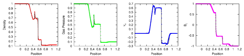
Figure 9: 2D shock tube results for the Brio & Wu (1988) adiabatic MHD test problem. The solid line shows the results using 10,000 grid cells on a 1D grid, and the points show results in 2D on a domain with $200\times 200$ cells at time $t=0.12$. The panels show (from left) gas density, pressure, normal velocity and tangential field. Note that because all points in the 2D domain are plotted, the number of points apparently contained within a discontinuity is larger than the actual number of points which resolve it.

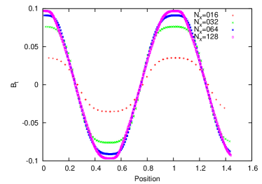
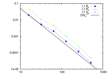
Figure 10: Circularly Polarised Alfvén Wave test. The left-hand plot shows the transverse magnetic field after advecting five times across the domain (initial amplitude 0.1) for models with resolutions $N_{x}=[16,32,64,128]$. The right-hand plot shows the L1 error (see equation 10) as a function of resolution for this test, obtained by comparing the initial to the final solution at each resolution. Second order convergence is clearly demonstrated.

Results from the following MHD test problems can be found at http://www.astro.uni-bonn.de/~jmackey/jmac/ together with the HD test problems. These adiabatic calculations are run using dimensionless units. The shock-tube tests of Brio & Wu (1988) and Falle et al. (1998) were performed in 1D and on a 2D grid with the shock-normal at an angle $\theta=\tan^{-1}0.5$ to the grid axes, ensuring that the problem is genuinely multi-dimensional. 2D Results are shown for the Brio & Wu (1988) test in Fig. 9 and are comparable to those obtained by Falle et al. (1998). The propagation of a polarised Alfvén wave was also calculated in 2D, using the initial conditions from Tóth (2000) and set up on a grid as in Stone et al. (2008). Running this test at different resolutions shows the degree of numerical diffusion in the algorithm and also the rate of convergence of the solution. Results are shown in Fig. 10; comparison of the first panel to results from Stone et al. (2008) shows that the third order Athena algorithm is significantly more accurate for this test at a given resolution, as expected. The second plot in this figure shows the L1 error:

$$L_{1}=\frac{1}{N}\sum_{i=0}^{N-1}\left|\phi_{i}-\phi_{i}^{0}\right|$$ (10)

for $N$ cells, where $\phi_{i}^{0}$ is the reference state for each cell and $\phi_{i}$ is the approximate numerical solution. This verifies that the code is indeed second order accurate for continuously differentiable density fields.

Results for the Orszag–Tang vortex problem (Orszag & Tang, 1979) were also very similar to those from the Athena code, with slightly more diffusion for smooth waves because of the lower order of accuracy.

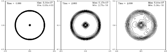
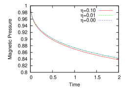
Figure 11: Field Loop Advection test: the initial (1st panel, from left) and final magnetic pressure is shown, with static (2nd panel) and advected (3rd panel) models. Only the central half of the domain is shown. 15 contours are shown on a linear scale from the minimum to maximum values (dimensionless units). Some extra diffusion and distortion is apparent in the advected model. The decay of magnetic pressure (normalised to the initial value) over time is shown in the 4th panel for a model run using the van Albada slope-limiter (van Albada et al., 1982). The three curves show the (small) effect of increasing artificial diffusion with the viscosity parameter (Falle et al., 1998) indicated.

The advection of a magnetic field loop (e.g. Stone et al., 2008) across a periodic domain is a challenging test for grid-based codes. When run with a non-zero velocity in the third dimension ($v_{z}\neq 0$) this test shows a weakness of the mixed-GLM divergence cleaning method – small divergence errors lead to small force errors and some of the initial magnetic field leaks unphysically into the $\hat{\mathbf{z}}$-direction ($\sim 5$ per cent). Results are shown in the first three panels of Fig. 11 for the evolution of the magnetic pressure. The left panel shows the initial conditions; the centre panel shows the state at $t=2$ for a model with no advection (to show the numerical diffusion), and the right panel shows the state at $t=2$ for a model advected twice across the domain. The time-decay of magnetic pressure for the advected models is shown in the right-most panel of Fig. 11. The constrained transport method employed in the Athena code, together with its third order accuracy, leads to less diffusion and a more symmetric solution to this problem than is obtained with our code (cf. Stone et al., 2008), but our results are comparable to those of other 2nd order astrophysics MHD codes. Tests also showed that for this test the van Albada slope-limiter (van Albada et al., 1982) produced a noticeably superior solution than the commonly used MinMod limiter, probably because the latter is significantly more diffusive.

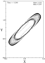
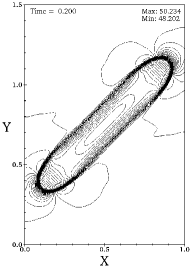
Figure 12: Contour plots of slices through the gas density (left) and magnetic pressure (right) at time $t=0.2$ for the MHD blast wave test problem with $\beta_{0}=0.002$. The slice is through the mid-plane $z=0.5$. There are 30 contours on a linear scale from the indicated minimum to maximum values. Because of the higher wavespeeds here compared to the $\beta_{0}=0.2$ model in Stone & Gardiner (2009), the fast magnetosonic waves seen in their results have long since left the domain in this simulation.

The expansion of a multi-dimensional adiabatic blast wave provides a good test of a code’s robustness in modelling 3D shocks and rarefactions. We ran the same 3D problem as described in Stone & Gardiner (2009, §6.5), with the gas pressure in a sphere at centre of the domain set to $100\times$ the ambient pressure, and with a uniform magnetic field at $45^{\circ}$ to the grid axes. Very similar results were found for the case where the initial plasma beta parameter $\beta=0.2$. Because of the robustness of the Dedner et al. (2002) algorithm, and presumably also because the integration algorithm used is slightly more diffusive than the Athena algorithm, our code can also simulate this test problem with a field $10\times$ stronger ($\beta=0.002$), shown in Fig. 12. This extra robustness is important for the strong field simulations run here.

Appendix B Boundary condition for mixed-GLM divergence cleaning algorithm

Dedner et al. (2002) suggest that for zero-gradient boundary conditions (BCs), using zero-gradient for the unphysical scalar field $\psi$ is sufficient. We have found, however, that more care is needed for magnetically dominated regions (plasma parameter $\beta\equiv 8\pi p_{g}/B^{2}\ll 1$) when gas is flowing subsonically near the boundary. In what follows $\hat{\mathbf{x}}$ is the normal vector to the boundary, the computational domain is ‘left’ of the boundary, and off the domain is ‘right’. Note that $\psi$ is not a physical variable so its gradient is not constrained. In fact if the field is constant across the boundary then the formal solution to the 1D Riemann problem is that the flux, $F[B_{x}]=0$ (as it is for all 1D Riemann problems). So ideally a boundary condition for $\psi$ should be selected which ensures $F[B_{x}]=0$. From Dedner et al. (2002, eqs. 41,42) it is easy to calculate this: the zero-gradient condition states that $B_{x}^{r}-B_{x}^{l}=0$ so if additionally $\psi^{r}=-\psi^{l}$ then $F[B_{x}]=0$ is obtained.

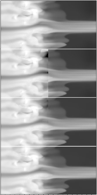
Figure 13: Plots of gas pressure on a log scale from $10^{-12}$–$10^{-8}\,\mathrm{dyne}\,.\mathrm{cm}^{-2}$, at time $t=12\,$kyr. Ionised gas has typical pressures of $10^{-8}\,\mathrm{dyne}\,.\mathrm{cm}^{-2}$ and neutral gas $10^{-11}\,\mathrm{dyne}\,.\mathrm{cm}^{-2}$. The top panel shows the full domain with $\psi^{r}=\psi^{l}$ as the BC. The second panel shows the same, but with a simulation of only the left half of the domain over-plotted to highlight the boundary effects, again with $\psi^{r}=\psi^{l}$. The third panel is as the second, but using $\psi^{r}=-\psi^{l}$ as the BC for both simulations, and the bottom panel shows the full domain with the $\psi^{r}=-\psi^{l}$ BC. The simulations were run using cooling model C2.

A sequence of figures from a 2D slab-symmetric test simulation (this time using c.g.s. units) are shown in Fig. 13 to demonstrate the effectiveness of the new boundary condition. The simulation domains used have sizes $[0.2,0.1]\,$pc (large) and $[0.1,0.1]\,$pc (small) and the radiation source is at infinity in the $-\hat{\mathbf{x}}$ direction. A group of randomly located dense clumps are placed between $x=0.02\,$pc and $x=0.08\,$pc on a uniform background density of $n_{\mathrm{H}}=100\,\mathrm{cm}^{-3}$. The initial magnetic field is $\mathbf{B}=[50,1,0]\times\sqrt{4\pi}\,\mu$G, and the initially constant gas pressure is set to give $\beta=0.017$ ($T=1500$K in the lowest density gas). Zero gradient BCs are enforced in the $\pm\hat{\mathbf{x}}$ directions, and periodic in $\pm\hat{\mathbf{y}}$.

Fig. 13 shows the gas pressure at time $t=12\,$kyr using cooling model C2. The problem with the zero-gradient BC for $\psi$ is very apparent, as is the dramatic improvement on switching to the $\psi^{r}=-\psi^{l}$ BC. The black regions are hiding cells which obtained negative pressures and were set to an artificial pressure floor value in order to allow the simulation to continue. Regarding the other boundaries, the $x=0.2\,$pc boundary only has waves moving perpendicular to it and so there is negligible net flow across the boundary. The $x=0\,$pc boundary has strong supersonic outflows, so the details of the BC for $\psi$ have little effect on it.

Appendix C Boundary effects as a function of domain size

Name	$x_{\mathrm{min}}$	$x_{\mathrm{max}}$	$y_{\mathrm{min}}$/$z_{\mathrm{min}}$	$y_{\mathrm{max}}$/$z_{\mathrm{max}}$	cells
Small	2.0	4.0	-0.75	0.75	$128\times 96^{2}$
Medium	1.5	4.5	-1.125	1.125	$192\times 144^{2}$
Large	1.5	5.5	-1.5	1.5	$256\times 192^{2}$
X-Long	1.5	6.5	-1.5	1.5	$320\times 192^{2}$
X-Wide	1.5	5.5	-2.0	2.0	$256^{3}$

Table 4: List of simulations run to test the boundary effects on the results of 3D MHD simulations of photoionisation. All tests were run with a $15\times\sqrt{4\pi}\simeq 53\,\mu$G magnetic field in the $y$–$z$ plane. Boundary positions are measured in parsecs in coordinates where the source is at $[0,0,0]$, as in Table 1.

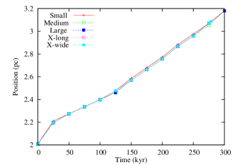
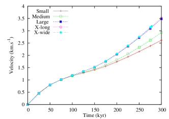
Figure 14: (1) Neutral mass, (2) Position of leading edge of ionisation front, and (3) mass-weighted mean neutral gas $x$-velocity. Note that the large, extra-long and extra-wide simulations have almost converged for all plots.

To study boundary effects on the results presented here, test simulations using clump configuration 1 were performed with increasingly larger domains, both in 2D and 3D with a medium perpendicular magnetic field (model R5 in Table 2). The same physical resolution was used for each simulation; boundary positions for five 3D simulations are listed in Table 4. Various global quantities were measured within the volume common to all simulations. Neutral mass, mean neutral gas velocity, and position of the first neutral cell on the domain are plotted as a function of time in Fig. 14. The small and medium simulations are clearly significantly affected by the boundaries whereas the large model is essentially identical to the X-long and X-wide models, indicating that the results have converged at least in this limited subdomain of the simulation. The position of the leading edge of the ionisation front is unaffected by the position of the boundaries, but the neutral gas mass and velocity are significantly affected. It was found that flow of gas through the distant boundary was impeded in these R-MHD simulations, something which did not happen in R-HD simulations.

References

- Arthur et al. (2010) Arthur S. J., Henney W. J., Mellema G., De Colle F., Vázquez-Semadeni E., 2010, MNRAS, submitted.
- Banerjee et al. (2009) Banerjee R., Vázquez-Semadeni E., Hennebelle P., Klessen R. S., 2009, MNRAS, 398, 1082
- Bertoldi (1989) Bertoldi F., 1989, ApJ, 346, 735
- Bertoldi & McKee (1990) Bertoldi F., McKee C. F., 1990, ApJ, 354, 529
- Bhatt (1999) Bhatt H. C., 1999, MNRAS, 308, 40
- Bhatt et al. (2004) Bhatt H. C., Maheswar G., Manoj P., 2004, MNRAS, 348, 83
- Bisbas et al. (2010) Bisbas T. G., Whitworth A. P., Wünsch R., Hubber D. A., Walch S., 2010, ArXiv e-prints
- Bodenheimer et al. (1979) Bodenheimer P., Tenorio-Tagle G., Yorke H. W., 1979, ApJ, 233, 85
- Bohigas et al. (2004) Bohigas J., Tapia M., Roth M., Ruiz M. T., 2004, AJ, 127, 2826
- Brandner et al. (2000) Brandner W., Grebel E. K., Chu Y., Dottori H., Brandl B., Richling S., Yorke H. W., Points S. D., Zinnecker H., 2000, AJ, 119, 292
- Brio & Wu (1988) Brio M., Wu C. C., 1988, Journal of Computational Physics, 75, 400
- Brogan & Troland (2001) Brogan C. L., Troland T. H., 2001, ApJ, 560, 821
- Cargo & Gallice (1997) Cargo P., Gallice G., 1997, Journal of Computational Physics, 136, 446
- Carlqvist et al. (2002) Carlqvist P., Gahm G. F., Kristen H., 2002, AP&SS, 280, 405
- Carlqvist et al. (2003) Carlqvist P., Gahm G. F., Kristen H., 2003, A&A, 403, 399
- Carlqvist et al. (1998) Carlqvist P., Kristen H., Gahm G. F., 1998, A&A, 332, L5
- de Hoffmann & Teller (1950) de Hoffmann F., Teller E., 1950, Physical Review, 80, 692
- Dedner et al. (2002) Dedner A., Kemm F., Kröner D., Munz C.-D., Schnitzer T., Wesenberg M., 2002, Journal of Computational Physics, 175, 645
- Downes & O’Sullivan (2009) Downes T. P., O’Sullivan S., 2009, ApJ, 701, 1258
- Esquivel & Raga (2007) Esquivel A., Raga A. C., 2007, MNRAS, 377, 383
- Falle et al. (1998) Falle S., Komissarov S., Joarder P., 1998, MNRAS, 297, 265
- Gahm et al. (2006) Gahm G. F., Carlqvist P., Johansson L. E. B., Nikolić S., 2006, A&A, 454, 201
- Garcia-Segura & Franco (1996) Garcia-Segura G., Franco J., 1996, ApJ, 469, 171
- Goodman et al. (1995) Goodman A. A., Jones T. J., Lada E. A., Myers P. C., 1995, ApJ, 448, 748
- Gritschneder et al. (2010) Gritschneder M., Burkert A., Naab T., Walch S., 2010, ApJ, 723, 971
- Gritschneder et al. (2009) Gritschneder M., Naab T., Walch S., Burkert A., Heitsch F., 2009, ApJL, 694, L26
- Henney et al. (2009) Henney W. J., Arthur S. J., de Colle F., Mellema G., 2009, MNRAS, 398, 157
- Henney et al. (2005) Henney W. J., Arthur S. J., García-Díaz M. T., 2005, ApJ, 627, 813
- Hester et al. (1996) Hester J. J., et al., 1996, AJ, 111, 2349
- Hummer (1994) Hummer D. G., 1994, MNRAS, 268, 109
- Indebetouw et al. (2007) Indebetouw R., Robitaille T. P., Whitney B. A., Churchwell E., Babler B., Meade M., Watson C., Wolfire M., 2007, ApJ, 666, 321
- Kessel-Deynet & Burkert (2003) Kessel-Deynet O., Burkert A., 2003, MNRAS, 338, 545
- Krumholz et al. (2007) Krumholz M., Stone J., Gardiner T., 2007, ApJ, 671, 518
- Kuiper et al. (2010) Kuiper R., Klahr H., Dullemond C., Kley W., Henning T., 2010, A&A, 511, A81
- Lasker (1966a) Lasker B. M., 1966a, ApJ, 143, 700
- Lasker (1966b) Lasker B. M., 1966b, ApJ, 146, 471
- Lee & Chen (2007) Lee H., Chen W. P., 2007, ApJ, 657, 884
- Lee et al. (2005) Lee H., Chen W. P., Zhang Z., Hu J., 2005, ApJ, 624, 808
- Lefloch & Lazareff (1994) Lefloch B., Lazareff B., 1994, A&A, 289, 559
- Lim & Mellema (2003) Lim A., Mellema G., 2003, A&A, 405, 189
- Lora et al. (2009) Lora V., Raga A. C., Esquivel A., 2009, A&A, 503, 477
- Mackey & Lim (2010) Mackey J., Lim A. J., 2010, MNRAS, 403, 714
- Marsh (1970) Marsh M. C., 1970, MNRAS, 147, 95
- Mellema et al. (2006b) Mellema G., Arthur S., Henney W., Iliev I., Shapiro P., 2006, ApJ, 647, 397
- Mellema et al. (2006a) Mellema G., Iliev I., Alvarez M., Shapiro P., 2006, New Astronomy, 11, 374
- Miao et al. (2006) Miao J., White G. J., Nelson R., Thompson M., Morgan L., 2006, MNRAS, 369, 143
- Molinari et al. (2010) Molinari S., et al., 2010, A&A, 518, L100
- O’Dell (2001) O’Dell C. R., 2001, ARA&A, 39, 99
- Oort & Spitzer (1955) Oort J. H., Spitzer Jr. L., 1955, ApJ, 121, 6
- Orszag & Tang (1979) Orszag S. A., Tang C., 1979, Journal of Fluid Mechanics, 90, 129
- Osterbrock (1989) Osterbrock D. E., 1989, Astrophysics of gaseous nebulae and active galactic nuclei. University Science Books, Mill Valley, CA
- Pellegrini et al. (2007) Pellegrini E. W., et al., 2007, ApJ, 658, 1119
- Pottasch (1958) Pottasch S. R., 1958, Bull. Astron. Inst. Netherlands, 14, 29
- Pound (1998) Pound M. W., 1998, ApJL, 493, L113
- Pound et al. (2007) Pound M. W., Kane J. O., Ryutov D. D., Remington B. A., Mizuta A., 2007, AP&SS, 307, 187
- Raga et al. (2009) Raga A. C., Henney W., Vasconcelos J., Cerqueira A., Esquivel A., Rodríguez-González A., 2009, MNRAS, 392, 964
- Redman et al. (1998) Redman M. P., Williams R. J. R., Dyson J. E., Hartquist T. W., Fernandez B. R., 1998, A&A, 331, 1099
- Ritzerveld (2005) Ritzerveld J., 2005, A&A, 439, L23
- Sandford et al. (1982) Sandford II M. T., Whitaker R. W., Klein R. I., 1982, ApJ, 260, 183
- Schmidt-Voigt & Koeppen (1987) Schmidt-Voigt M., Koeppen J., 1987, A&A, 174, 211
- Smith et al. (2010a) Smith N., Bally J., Walborn N. R., 2010a, MNRAS, 405, 1153
- Smith & Brooks (2007) Smith N., Brooks K. J., 2007, MNRAS, 379, 1279
- Smith et al. (2010b) Smith N., et al., 2010b, MNRAS, 406, 952
- Spitzer (1998) Spitzer L., 1998, Physical Processes in the Interstellar Medium. Wiley
- Sridharan et al. (1996) Sridharan T. K., Bhatt H. C., Rajagopal J., 1996, MNRAS, 279, 1191
- Stone & Gardiner (2009) Stone J., Gardiner T., 2009, New Astronomy, 14, 139
- Stone et al. (2008) Stone J., Gardiner T., Teuben P., Hawley J., Simon J., 2008, ApJS, 178, 137
- Sugitani et al. (2007) Sugitani K., et al., 2007, PASJ, 59, 507
- Tóth (2000) Tóth G., 2000, Journal of Computational Physics, 161, 605
- van Albada et al. (1982) van Albada G. D., van Leer B., Roberts Jr. W. W., 1982, A&A, 108, 76
- Voronov (1997) Voronov G. S., 1997, Atomic Data and Nuclear Data Tables, 65, 1
- Whalen & Norman (2008) Whalen D., Norman M., 2008, ApJ, 672, 287
- White et al. (1999) White G. J., et al., 1999, A&A, 342, 233
- Williams et al. (2001) Williams R., Ward-Thompson D., Whitworth A., 2001, MNRAS, 327, 788
- Williams (2002) Williams R. J. R., 2002, MNRAS, 331, 693
- Williams (2007) Williams R. J. R., 2007, AP&SS, 307, 179
- Williams & Dyson (2001) Williams R. J. R., Dyson J. E., 2001, MNRAS, 325, 293
- Williams et al. (2000) Williams R. J. R., Dyson J. E., Hartquist T. W., 2000, MNRAS, 314, 315
- Williams & Henney (2009) Williams R. J. R., Henney W. J., 2009, MNRAS, 400, 263
- Yorke (1986) Yorke H. W., 1986, ARA&A, 24, 49