NGC 1866: a milestone for understanding the chemical evolution of stellar populations in the LMC

Abstract

We present new FLAMES@VLT spectroscopic observations of 30 stars in the field of the LMC stellar cluster NGC 1866. NGC 1866 is one of the few young and massive globular cluster that is close enough so that its stars can be individually studied in detail. Radial velocities have been used to separate stars belonging to the cluster and to the LMC field and the same spectra have been used to derive chemical abundances for a variety of elements, from [Fe/H] to the light (i.e. Na, O, Mg…) to the heavy ones. The average iron abundance of NGC 1866 turns out to be [Fe/H]= –0.43$\pm$0.01 dex (with a dispersion $\sigma$= 0.04 dex), from the analysis of 14 cluster-member stars. Within our uncertainties, the cluster stars are homogeneous, as far as chemical composition is concerned, independent of the evolutionary status. The observed cluster stars do not show any sign of the light elements ’anti-correlation’ present in all the Galactic globular clusters so far studied, and also found in the old LMC stellar clusters. A similar lack of anti-correlations has been detected in the massive intermediate-age LMC clusters, indicating a different formation/evolution scenario for the LMC massive clusters younger than $\sim$ 3 Gyr with respect to the old ones.
Also opposite to the Galactic globulars, the chemical composition of the older RGB field stars and of the young post-MS cluster stars show robust homogeneity suggesting a quite similar process of chemical evolution. The field and cluster abundances are in agreement with recent chemical analysis of LMC stars, which show a distinctive chemical pattern for this galaxy with respect to the Milky Way. We discuss these findings in light of the theoretical scenario of chemical evolution of the LMC.

1 Introduction

The role of the Large Magellanic Cloud (LMC) as an exceptional laboratory for the study of stellar populations and stellar evolution has been early recognized by many authors (e.g. Hodge, 1960, 1961; van den Bergh & Hagen, 1968; van den Bergh & de Boer, 1984). The star formation history and the related chemical evolution in the LMC have been studied through extensive photometric surveys (see e.g. Harris & Zaritsky, 2009) and theoretically through detailed modeling (Matteucci & Brocato, 1990). The advent of the 8 m VLT telescopes has opened a new era in the investigation of resolved stellar populations, by producing high quality/high resolution spectra, which allow the detailed chemical study of many single hot and cool stars in different regions of the LMC (see e.g. Pompeia et al., 2008). One of the most distinctive results of these studies is that, similarly to other nearby dwarf galaxies, the LMC shows clear signatures of a different chemical evolution with respect to the chemical evolution of the Milky Way sub-population components (Venn et al., 2004).

Another fundamental characteristic of the LMC is that its cluster population covers a wide metallicity distribution and contains a large population of massive objects covering a wide age range, which provide a unique opportunity of studying rich samples of intermediate mass stars ($\sim$ 3-8 $M_{\odot}$) and the details of their evolutionary phases. A large and still ongoing effort has been done to collect photometric and spectroscopic data of stars in the stellar clusters of this galaxy (Hill et al., 2000; Pompeia et al., 2005; Johnson et al., 2006; Mucciarelli et al., 2008b, 2009, 2010; Tolstoy, Hill & Tosi, 2009).

In this scenario, NGC 1866 can be considered as a milestone for understanding the chemical evolution of the youngest stellar populations in the LMC, because this cluster is extremely rich ($\sim 5\times 10^{4}$ $M_{\odot}$) compared with the coeval LMC clusters, with an age of $\sim 10^{8}yr$ and mass of $\sim$ 5 $M_{\odot}$ for the stars evolving off the Main Sequence (MS) (Brocato et al., 2003) and a metallicity close to the one of 47 Tuc. Concerning its metal content, the only study based on high-resolution spectra is that by Hill et al. (2000), including Fe, O and Al abundances for three member stars of the cluster, providing an iron abundance of [Fe/H]= –0.50$\pm$0.1 dex, a solar abundance of [O/Fe] and a mild depletion of [Al/Fe] with respect to the solar value.

Thus, high resolution spectroscopy properly coupled with a high quality color magnitude diagram (CMD) of NGC 1866 represent a unique tool to probe our knowledge of nucleosynthesis and mixing processes in intermediate mass stars during their evolution off of the MS. A further advantage of studying this cluster is that LMC field stars can be easily identified as Red Giant Branch (RGB) stars, and a comparison between the abundances of these RGB field stars with those for the young cluster stars will be very powerful to infer the chemical evolution processes in the LMC stellar population around the cluster and inside the cluster itself. We take advantage of the large database of photometric data available for NGC 1866 and the related comparison with theoretical isochrones (Brocato et al., 2003), and combine it with new high resolution spectra obtained at the VLT of stars well identified in the CMD of the LMC cluster NGC 1866 and its field. The paper is arranged as follows. The observations are described in the next section, while the assumptions on the stellar atmospheres are presented in Section 3. The chemical analysis and the related uncertainties are discussed in Section 4 and 5 and the results on the abundances of the elements are reported in section 6. Section 7 provides a general discussion on the observed framework, a brief summary concludes the paper.

2 Observational material

The spectroscopic data set analyzed here has been obtained with the FLAMES spectrograph (Pasquini et al., 2002) at VLT Kueyen 8.2 m telescope, in the combined UVES+GIRAFFE mode, allowing the simultaneous observation of 8 stars with the Red Arm of UVES at high-resolution (R$\sim$42000) and of 132 with GIRAFFE mid-resolution (R$\sim$20000-25000) fibers. All the observations have been performed in Service Mode during 7 nights between October 2004 and January 2005 under proposal 074.D-0305(A).
We used three different setups for the GIRAFFE observations:
(1) HR11 — R=24200, $\Delta\lambda$=5597-5840 $\mathring{A}$;
(2) HR12 — R=18700, $\Delta\lambda$=5821-6146 $\mathring{A}$;
(3) HR13 — R=22500, $\Delta\lambda$=6120-6405 $\mathring{A}$.
The adopted GIRAFFE set-ups provide a spectral coverage ($\sim$5600-6400 $\mathring{A}$) including several absorption lines of key elements such as iron, $\alpha$, iron-peak and neutron-capture elements. All the targets have been observed in these three setups, with a time exposure of 3600 sec for each individual exposure (5 for HR11, 4 for HR12 and 3 for HR13), realizing a global S/N ratio between 40 and 100 (per pixel) at $\sim$6000 $\mathring{A}$. The spectra have been reduced by the standard FLAMES reduction pipeline which includes bias subtraction, flat-fielding, wavelength calibration with a reference Th-Ar calibration lamp and final extraction of the 1-dimensional spectra.

The radial velocity of each spectrum has been derived with the cross-correlation task of the BLDRS (GIRAFFE Base-Line Data Reduction Software ), while for the stars observed with UVES the radial velocity has been estimated by measuring the centroids of several tens of un-blended lines. Heliocentric corrections have been computed by using the IRAF task RVCORRECT. The stars with $v_{helio}<$200 km $s^{-1}$ have been discarded because they likely belong to our Galaxy, according to the radial velocity maps computed for the LMC by Staveley-Smith et al. (2003). We obtained an average heliocentric velocity for the cluster of $v_{helio}$=298.5$\pm$0.4 km $s^{-1}$ ($\sigma$=1.6 km $s^{-1}$) by using 16 stars, in good agreement with the previous determination by Hill et al. (2000) of $v_{helio}$=299.8$\pm$0.5 km $s^{-1}$ ($\sigma$=1.4 km $s^{-1}$). In the computation of the average radial velocity we have excluded three observed Cepheid stars. Moreover, 11 RGB stars belonging to the LMC field have been observed, with $v_{helio}$ ranging from 261.4 to 305.5 km $s^{-1}$. All the individual exposures have been sky-subtracted, shifted to zero-velocity, then co-added and normalized to unity. Fig. 1 shows the CMD in the V-(B-V) plane of NGC 1866 with the positions of our target stars: big grey circles indicate the stars member of NGC 1866 (according to their $v_{helio}$ value, distance and position in the CMD), grey triangles are the observed LMC field stars and grey squares the Cepheids. Information about all observed targets is listed in Tab. LABEL:info with ID number (Musella et al., 2006), RA, Dec, the V and K magnitudes, heliocentric radial velocities and S/N ratio (computed at $\sim$6000 $\mathring{A}$). The total sample consists of 30 stars, of which 19 are from the cluster and 11 from the LMC field. The three cluster Cepheids will be discussed in a forthcoming paper.

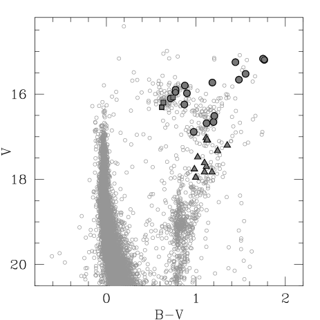
Figure 1: Color-Magnitude Diagram of NGC 1866 (Musella et al., 2006) with marked the observed target stars: the cluster-member stars and the LMC field stars analyzed in this work are marked respectively as filled circles and triangles. Squares indicate the observed Cepheid stars.

Table 1: Target information: ID number, RA, Dec, V and K magnitudes, heliocentric radial velocities, S/N and membership.

ID-Star	RA	Dec	V	K	$v_{helio}$	S/N	Membership	Notes
	(J2000)	(J2000)			(km$s^{-1})$
652	78.384167	–65.509056	17.76	15.02	292.9	40	FIELD
1025	78.342208	–65.503500	16.20	14.60	294.9	80	CLUSTER	Cepheid — HV12197
1146	78.366417	–65.501639	15.20	10.94	299.0	120	CLUSTER	UVES — TiO bands
1491	78.450708	–65.497028	17.95	15.46	267.3	45	FIELD
1605	78.282292	–65.495417	17.33	14.37	266.7	45	FIELD
1969	78.354708	–65.491444	16.31	14.66	311.0	90	CLUSTER	Cepheid — HV12199
1995	78.533833	–65.491222	17.08	14.40	280.3	50	FIELD
2131	78.449917	–65.489694	15.66	12.25	299.1	100	CLUSTER
2305	78.357125	–65.487639	17.61	14.79	272.2	45	FIELD
2981	78.403542	–65.481611	15.52	11.95	301.3	100	CLUSTER	UVES
4017	78.334708	–65.474111	16.51	13.72	298.7	70	CLUSTER
4209	78.347917	–65.472972	17.20	13.96	270.8	60	FIELD
4425	78.374708	–65.471500	15.73	12.98	299.3	90	CLUSTER
4462	78.497500	–65.471333	15.80	13.78	298.8	80	CLUSTER
5231	78.411667	–65.466500	15.24	11.86	298.1	100	CLUSTER
5415	78.435583	–65.465194	15.90	14.02	297.6	90	CLUSTER
5579	78.421167	–65.464028	16.09	13.94	291.7	90	CLUSTER	Cepheid — We2
5706	78.454875	–65.463028	16.65	13.83	298.5	80	CLUSTER
5789	78.413625	–65.462389	15.97	13.80	297.2	90	CLUSTER
5834	78.443333	–65.462056	15.17	10.78	296.0	120	CLUSTER	UVES — TiO bands
7111	78.476333	–65.451861	17.83	15.11	261.4	40	FIELD
7392	78.422375	–65.449361	15.95	14.06	297.9	85	CLUSTER
7402	78.361208	–65.449250	16.88	14.53	297.8	60	CLUSTER
7415	78.433625	–65.449167	16.24	14.14	302.2	70	CLUSTER
7862	78.458417	–65.444750	16.68	13.99	297.2	60	CLUSTER
9256	78.489750	–65.428778	17.48	15.09	293.4	40	FIELD
9649	78.509167	–65.424056	17.02	14.43	272.1	60	FIELD
10144	78.482625	–65.415944	17.83	14.90	273.2	50	FIELD
10222	78.530208	–65.414583	17.70	14.81	305.5	40	FIELD
10366	78.430875	–65.412111	16.10	14.36	296.7	60	CLUSTER

3 Atmospheric parameters

Initial atmospheric parameters have been computed from the photometric data. Effective temperatures ($T_{eff}$) for the target stars have been derived from de-reddened (V-K) color, obtained by combining the visual FORS1 photometry (Musella et al. (2006), Musella et al. 2010, in preparation) and the near-infrared SOFI photometry (Mucciarelli et al., 2006). We assumed a reddening value of E(B-V) =0.064 by Walker et al. (2001), the extinction law by Rieke & Lebofsky (1985) and using the empirical $(V-K)_{0}$-$T_{eff}$ calibration computed by Alonso et al. (1999) and based on the Infrared Flux Method; transformations between the different photometric systems have been performed by means of the relations by Carpenter (2001) and Alonso et al. (1998).

Surface gravities have been obtained from the classical equation

$$log~{}(g/g_{\odot})=4\cdot log(T_{eff}/T_{eff,\odot})$$

$$+log~{}(M/M_{\odot})-0.4\cdot(M_{bol}-M_{bol,\odot})$$

by adopting a distance modulus of $(m-M)_{0}$= 18.50, the bolometric corrections computed by Alonso et al. (1999). We consider a mass of $M_{1866}$= 4.5 $M_{\odot}$ (according to the cluster age inferred by Brocato et al., 2003) for the cluster-member stars and of $M_{LMC-Field}$= 1.5 $M_{\odot}$ (corresponding to the typical evolutive mass of a population of $\sim$2 Gyr) for the LMC field stars. We checked that photometric $T_{eff}$ and log g well satisfy the excitation and ionization equilibrium, respectively; hence the neutral iron abundance must be independent by the excitation potential $\chi$, while neutral and single ionized iron lines may provide the same abundance within the quoted errors.

Generally, the adopted temperature scale well satisfies the excitation equilibrium and only a few field stars require re-adjusted temperatures. To better constrain the gravity values, we imposed the condition of [Fe/H]  I=[Fe/H] II. Photometric and spectroscopic gravities for the cluster stars are consistent, while for the field stars we needed to re-adjust the gravities within $\pm$0.3 dex, probably due to incorrect assumptions for their mass, reddening and/or distance modulus.

In order to estimate the micro-turbulent velocity $v_{t}$ we adopted as initial value a velocity of $v_{t}$=1.5 km $s^{-1}$ and we adjusted this parameter in each star in order to minimize the trend between [Fe/H] I abundance and the expected line strength, defined as $\lg{gf}-\theta\chi$ (where $\theta$ is 5040/$T_{eff}$), according to the prescriptions by Magain (1984) and imposing in this way that strong and weak lines give the same abundance.
The final atmospheric parameters (and the derived [Fe/H] abundance ratios) are listed in Tab. LABEL:param.

Uncertainties in the derived atmospheric parameters have been computed by taking into account the main sources of errors. For $T_{eff}$, we considered uncertainties in the photometric (V-K) colors and reddening, finding uncertainties ranging from $\sim$70 to $\sim$120 K; in the following we assume a typical error of 100 K. The uncertainties in the gravities have been computed by considering the corresponding error in $T_{eff}$ (being log g fixed by the choice of $T_{eff}$) and in the adopted reddening and mass. In particular, the error in the adopted mass is small for the cluster stars (for which the age is well constrained, see e.g. Brocato et al., 2003), while for the field stars we assume an error of the order of $\sim$30%. Typical errors in gravities are of the order of 0.2. The errors in $v_{t}$ have been estimated by varying this parameter until the $\sigma_{slope}$ value for the slope in the line strength–A(Fe) plane is reached. Because $v_{t}$ is estimated spectroscopically, the associated errors depend on the SNR of the spectra and the number of adopted lines: we find that the errors in $v_{t}$ ranging from $\sim$0.15 km/s for the cluster stars to $\sim$0.3 km/s for the faintest field stars.

Table 2: Atmospheric parameters and iron content for all the target stars.

ID-Star	$T_{eff}$	log g	$v_{t}$	[Fe/H]
	(K)		(km$s^{-1})$	(dex)
		CLUSTER
2131	4080	1.05	2.0	–0.47
2981	3870	0.90	1.9	–0.45
4017	4490	1.70	1.8	–0.47
4425	4530	1.45	1.8	–0.43
4462	5320	1.90	1.7	–0.39
5231	4100	0.90	2.1	–0.48
5415	5540	2.05	1.5	–0.42
5706	4460	1.80	1.8	–0.38
5789	5110	1.90	1.5	–0.43
7392	5510	1.60	1.7	–0.38
7402	4900	2.10	1.5	–0.46
7415	5200	2.05	1.7	–0.49
7862	4570	1.90	1.7	–0.46
10366	5760	2.20	1.7	–0.38
		FIELD
652	4530	1.90	1.4	–0.71
1491	4760	2.00	1.5	–0.44
1605	4360	1.50	1.5	–0.85
1995	4580	2.00	1.5	–1.15
2305	4470	1.75	1.5	–0.60
4209	4180	1.30	1.5	–0.63
7111	4550	1.90	1.4	–0.59
9256	4870	2.30	1.6	–0.33
9649	4660	2.05	1.4	–0.32
10144	4390	1.80	1.4	–0.75
10222	4420	1.75	1.3	–0.52

4 Chemical analysis

For each star a plane-parallel, one-dimensional, LTE model atmosphere has been computed by using the ATLAS 9 code (Kurucz, 1993a) in its Linux version (Sbordone et al., 2004) and adopting the atmospheric parameters described in Tab. LABEL:param. We used the new Opacity Distribution Functions by Castelli & Kurucz (2003), with a solar-scaled chemical mixture (according with the previous chemical analysis of NGC 1866 by Hill et al., 2000), micro-turbulent velocity of 1 km $s^{-1}$, a mixing-length parameter of 1.25 and no approximate overshooting.

For the chemical analysis of our sample we resort to the line profile fitting technique, comparing the observed line profile with suitable synthetic ones. The adopted code (described in detail in Caffau et al., 2005) performs a $\chi^{2}$ minimization of the deviation between synthetic profiles and the observed spectrum. The best fitting spectrum is obtained by linear interpolation between three synthetic spectra which differ only in the abundance of a given element; the minimum $\chi^{2}$ is computed numerically by using the MINUIT package (James, 1998). All the synthetic spectra were computed with the SYNTHE code (Kurucz, 1993b). Fig. 2 shows examples of final best-fit for used spectral features in the GIRAFFE spectrum of the star #2131 (upper panel) and in the UVES spectrum of the star #2981 (lower panel); synthetic spectra with abundances of $\pm$0.1 dex with respect to the best fit abundance are also plotted for sake of comparison.

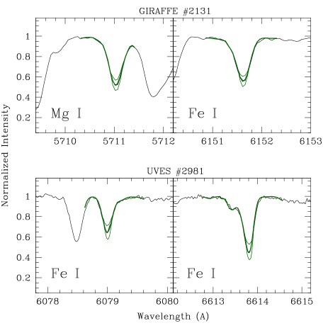
Figure 2: Portions of spectrum for the two observed stars #2131 (upper panels, GIRAFFE) and #2891 (lower panels, UVES) with overplotted the best fit (green, thick lines). Synthetic spectra with abundances of $\pm$0.1 dex with respect to the best fit spectra are also plotted as green, thin lines.

We select a set of spectral lines (predicted to be un-blended by the inspection of preliminary synthetic spectra computed with the photometric atmospheric parameters) and adopting accurate laboratory or theoretical oscillator strengths whenever possible. In the computation of synthetic spectra we employ the line-list of R. L. Kurucz database , updating the oscillator strengths where available. Hyperfine splitting has been included for Mn I, Cu I, Ba II, La II and Eu II lines. Briefly, we summary in the following the updated atomic data:
O I – for the forbidden [O] I transition at 6300.31 $\mathring{A}$ we use the Storey & Zeippen (2000) oscillator strength, while for the blended Ni I line at 6300.34 $\mathring{A}$ we adopt the Johansson et al. (2003) laboratory log gf;
Mg I – we use the Gratton et al. (2003) log gf for the Mg I transitions at 5711.09, 6318.71 and 6319.24 $\mathring{A}$;
Mn I – hyperfine splitting from R. L. Kurucz website are employed;
Cu II – for the 5782.0 $\mathring{A}$ line the hyperfine levels are from Cunha et al. (2002), adopting a solar isotopic mixture;
Ba II – we use the hyperfine components by Prochaska et al. (2000) for the Ba II lines at 5853.7, 6141.6 and 6496.9 $\mathring{A}$;
Rare earths – the transition probability of the 6043.4 Ce II line is from DREAM Database and of the 5740.8 Nd II line by Den Hartog et al. (2003);
La II and Eu II – hyperfine splitting is included, by adopting the recent atomic data by Lawler et al. (2001a) and Lawler et al. (2001b) for Eu II and La II respectively. We perform the calculation of their hyperfine structure with the LINESTRUC code, described by Wahlgren (2005).

The Na lines are affected by NLTE effects and such corrections are a function of line strength, metallicity, temperature and gravity. We correct our Na abundances for departures from LTE, interpolating the grid by Gratton et al. (1999).

All the abundances are referred to the solar values listed in the recent compilation by Lodders, Palme & Gail (2009), adopting only for O and Eu the new solar abundances by Caffau et al. (2008) and Mucciarelli et al. (2008a), respectively, and for Mg, Al and Cu the values derived from our solar analysis. For sake of homogeneity, we perform an analysis of the solar spectrum by using the same procedure adopted here. We study the Kurucz flux spectrum and employ the ATLAS 9 solar model atmosphere computed by F. Castelli . Generally, we find that our solar analysis nicely agrees with the solar values by Lodders, Palme & Gail (2009) within the uncertainties. We note that only for few elements there are relevant differences with respect to the values by Lodders, Palme & Gail (2009). Our solar Mg abundance is of 7.43, while Lodders, Palme & Gail (2009) recommended value is of of 7.54; such a discrepancy on the line selection can be attributed to the adopted log gf, as discussed by Gratton et al. (2003). Al abundance is of 6.21 from the doublet at 6696–98 $\mathring{A}$ (0.26 dex lower than the value listed by Lodders, Palme & Gail (2009)), probably due to NLTE effects that affect these lines and/or imprecise log gf values . Finally, our Cu solar abundance is 0.2 dex lower than the reference value. Such a difference has been already noted by Cunha et al. (2002) and ascribed to the differing log gf values and model atmospheres.

5 Error budget

In the case of observed spectra, where adjacent pixels are not completely independent of each other, the error associated to the $\chi^{2}$ minimization cannot be derived by the $\chi^{2}$ theorems (see Cayrel et al., 1999; Caffau et al., 2005). In order to estimate the uncertainties related to the fitting procedure we resort to Monte Carlo simulations. We choose to study some cluster stars, which we consider as representative of the different S/N and atmospheric parameters sampled by our targets: the stars #2131 and #10366, located in the red giant region and in the blue side of the Blue Loop of NGC 1866, respectively, and the field RGB star #652. We injected Poisson noise into the best-fit synthetic spectrum of some iron lines, according to the standard deviation used in the fitting and we performed the fit with the same procedure described above. For each line we performed a total of 10000 Monte Carlo events. From the resulting abundance distributions we may estimate a 1$\sigma$ level for normal distributions. The two cluster stars exhibit similar Monte Carlo distributions. We claim that the abundances derived by our fitting procedure are constrained within $\pm$0.09 dex. We repeated the same procedure for #652 (the star with the lowest S/N of the sample, S/N= 40), estimating that the 68% of the events is comprised within 0.15 dex.

We computed for the stars #2131 and #10366 the sensitivity of each abundance ratio to variation of the atmospheric parameters. We assume typical errors for each parameter according to Section 3. Tab. LABEL:error lists the variations of the abundance ratios by varying each time one only parameter and their sum in quadrature can be considered a conservative estimate of the systematic error associated to a given abundance ratio.

Table 3: Variations in the abundances of two stars #2131 and #10366 due to the uncertainties in the atmospheric parameters. The adopted parameters variations are also reported.

		#2131			#10366
Ratio	$T_{eff}$	log g	$v_{t}$	$T_{eff}$	log g	$v_{t}$
	(100 K)	(0.2)	(0.3 km/s)	(100 K)	(0.2)	(0.3 km/s)
$[Fe/H]$	–0.06	0.02	-0.03	–0.04	–0.01	–0.05
$[Na/Fe]$	–0.05	0.03	–0.08	–0.03	–0.03	–0.10
$[O/Fe]$	0.05	–0.04	–0.05	0.04	–0.05	–0.07
$[Mg/Fe]$	–0.04	0.04	0.04	0.04	0.01	0.02
$[Si/Fe]$	–0.06	0.03	0.02	–0.05	0.04	0.03
$[Ca/Fe]$	0.02	–0.06	0.03	0.05	–0.06	0.04
$[Ti/Fe]$	0.12	0.03	0.10	0.11	–0.01	0.12
$[Mn/Fe]$	–0.15	0.04	0.08	–0.08	0.06	0.12
$[Ni/Fe]$	-0.03	–0.02	0.02	–0.02	0.02	0.03
$[Cu/Fe]$	-0.07	0.06	0.08	0.05	0.09	0.05
$[Y/Fe]$	–0.04	0.07	0.04	0.03	0.05	0.03
$[Zr/Fe]$	0.14	0.04	0.03	0.12	–0.04	–0.02
$[Ba/Fe]$	0.04	0.06	0.12	0.05	0.08	0.10
$[La/Fe]$	0.02	0.03	0.04	0.03	–0.02	0.01
$[Ce/Fe]$	0.02	0.03	–0.02	–0.04	-0.01	0.01
$[Nd/Fe]$	0.03	0.08	0.03	0.01	0.06	0.04

6 Results

Tab. LABEL:cl and LABEL:fld list the derived abundance ratios for all the samples of stars (cluster and field respectively) and Tab. LABEL:aver the average values (with the corresponding dispersion by the mean) obtained for NGC 1866. Two of the targets (namely #1146 and #5834) are affected by strong TiO bands, thus have not been analyzed due to the severe molecular absorption conditions. It is worth noting that the dispersion by the mean for each abundance ratio in NGC 1866 is consistent within the uncertainties arising from the fitting procedure and the atmospheric parameters, pointing toward a general homogeneity for all the studied elements based on more than a single star (see Section 6.5).

In Fig. 3 a full picture of the chemical abundances inferred from our sample is shown: blue squares are the average values for NGC 1866 and red triangles for the LMC field stars. In Fig. 4–9 we summarize the derived abundances of our sample for some interesting elements (filled grey points for the field stars and grey large square for the average value of the stars of NGC 1866), comparing these results with other databases based on high-resolution spectroscopy for the Galactic stars (empty grey points, by Edvardsson et al., 1993; Burris et al., 2000; Fulbright, 2000; Reddy et al., 2003; Gratton et al., 2003; Reddy et al., 2006), the LMC field stars (blue points by Smith et al., 2002; Pompeia et al., 2008) and the LMC globular clusters (blue squares by Johnson et al., 2006; Mucciarelli et al., 2008b, 2010).

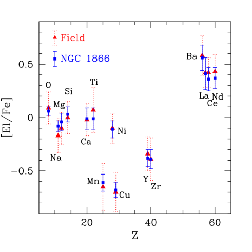
Figure 3: Comparison between the mean spectroscopic values of stars belonging to NGC 1866 (blue squares) and the surrounding field (red triangles). Errorbars indicate the dispersion by the mean.

Table 4: Abundances ratios for the target stars of NGC 1866. The numbers in brackets indicate the number of used lines.

ID-Star	[Na/Fe]	[O/Fe]	[Mg/Fe]	[Si/Fe]	[Ca/Fe]	[Ti/Fe]	[Ni/Fe]	[Mn/Fe]
	(dex)	(dex)	(dex)	(dex)	(dex)	(dex)	(dex)	(dex)
2131	–0.09 (4)	0.11 (1)	0.03 (3)	0.02 (4)	–0.13 (8)	–0.08 (8)	–0.13 (10)	–0.58 (3)
2981	–0.12 (4)	0.10 (1)	–0.04 (3)	0.09 (4)	–0.12 (10)	–0.13 (11)	–0.05 (11)	–0.69 (3)
4017	–0.07 (4)	0.01 (1)	–0.12 (3)	0.03 (6)	–0.02 (8)	–0.05 (10	–0.16 (8)	–0.55 (3)
4425	–0.11 (4)	0.13 (1)	–0.09 (3)	0.09 (5)	0.05 (6)	0.14 (6)	–0.13 (8)	–0.56 (3)
4462	–0.03 (4)	0.09 (1)	0.02 (3)	–0.04 (4)	–0.01 (8)	–0.02 (6)	0.04 (12)	–0.55 (3)
5231	–0.13 (4)	0.00 (1)	–0.01 (3)	–0.07 (5)	–0.16 (9)	–0.04 (8)	–0.17 (10)	–0.61 (3)
5415	–0.11 (4)	0.03 (1)	–0.08 (3)	0.20 (5)	0.14 (8)	0.25 (8)	–0.20 (8)	–0.63 (3)
5706	–0.19 (4)	0.11 (1)	–0.03 (3)	0.08 (5)	–0.17 (7)	–0.15 (8)	–0.12 (7)	–0.66 (3)
5789	–0.02 (4)	0.07 (1)	–0.07 (3)	–0.06 (4)	0.10 (8)	–0.03 (7)	–0.03 (6)	–0.81 (3)
7392	–0.12 (4)	0.04 (1)	0.10 (3)	–0.02 (5)	0.11 (6)	–0.03 (8)	–0.12 (8)	–0.62 (3)
7402	–0.10 (4)	0.09 (1)	–0.17 (3)	0.03 (5)	0.04 (6)	0.05 (9)	–0.04 (8)	–0.60 (3)
7415	–0.04 (4)	0.06 (1)	0.02 (3)	0.06 (4)	–0.12 (7)	0.00 (5)	–0.13 (11)	–0.51 (3)
7862	–0.11 (4)	0.10 (1)	–0.16 (3)	0.08 (4)	–0.01 (8)	–0.04 (6)	0.00 (10)	–0.64 (3)
10366	–0.02 (4)	0.02 (1)	–0.09 (3)	0.07 (5)	0.00 (8)	–0.04 (8)	–0.23 (9)	–0.48 (3)
ID-Star	[Cu/Fe]	[Y/Fe]	[Zr/Fe]	[Ba/Fe]	[La/Fe]	[Ce/Fe]	[Nd/Fe]	[Fe/H]
	(dex)	(dex)	(dex)	(dex)	(dex)	(dex)	(dex)	(dex)
2131	–0.76 (1)	–0.22 (2)	–0.52 (3)	0.52 (2)	0.37 (1)	0.25 (1)	0.51 (3)	–0.47 (42)
2981	—	–0.45 (5)	–0.51 (4)	0.54 (3)	0.44 (1)	0.41 (3)	0.52 (8)	–0.45 (89)
4017	–0.67 (1)	–0.39 (1)	–0.21 (3)	0.55 (2)	0.60 (1)	0.20 (1)	0.37 (3)	–0.47 (40)
4425	–0.69 (1)	–0.33 (2)	–0.41 (3)	0.63 (2)	0.33 (1)	0.29 (1)	0.24 (3)	–0.43 (38)
4462	–0.70 (1)	–0.33 (2)	—	—	0.40 (1)	0.25 (1)	0.38 (3)	–0.39 (44)
5231	–0.70 (1)	–0.53 (1)	–0.49 (3)	0.51 (2)	0.36 (1)	0.17 (1)	0.47 (2)	–0.48 (40)
5415	–0.69 (1)	–0.36 (2)	–0.38 (2)	—	0.18 (1)	0.41 (1)	0.23 (3)	–0.42 (37)
5706	–0.75 (1)	–0.49 (2)	–0.46 (3)	0.48 (2)	0.35 (1)	0.28 (1)	0.24 (2)	–0.38 (39)
5789	–0.57 (1)	—	–0.33 (3)	0.64 (2)	0.20 (1)	0.44 (1)	—	–0.43 (39)
7392	–0.60 (1)	–0.44 (2)	—	0.61 (2)	0.18 (1)	0.19 (1)	0.38 (2)	–0.38 (42)
7402	–0.58 (1)	–0.43 (2)	–0.40 (3)	0.58 (2)	0.39 (1)	0.20 (1)	0.45 (3)	–0.46 (40)
7415	–0.82 (1)	–0.38 (2)	–0.44 (3)	0.55 (2)	0.60 (1)	0.27 (1)	0.32 (3)	–0.49 (42)
7862	–0.71 (1)	–0.43 (2)	–0.42 (3)	0.46 (2)	0.42 (1)	0.17 (1)	0.34 (3)	–0.46 (37)
10366	—	–0.42 (1)	—	0.62 (2)	0.67 (1)	0.51 (1)	0.36 (3)	–0.38 (40)
ID-Star	[Al/Fe]	[Mo/Fe]	[Ru/Fe]	[Hf/Fe]	[W/Fe]	[Pr/Fe]	[Eu/Fe]	[Er/Fe]
	(dex)	(dex)	(dex)	(dex)	(dex)	(dex)	(dex)	(dex)
2981	–0.30 (2)	–0.03 (2)	–0.05 (1)	0.17 (2)	0.02 (1)	0.51 (5)	0.57 (1)	0.30 (2)

Table 5: Abundance ratios of the LMC field target stars. The numbers in brackets indicate the number of used lines.

ID-Star	[Na/Fe]	[O/Fe]	[Mg/Fe]	[Si/Fe]	[Ca/Fe]	[Ti/Fe]	[Ni/Fe]	[Mn/Fe]
	(dex)	(dex)	(dex)	(dex)	(dex)	(dex)	(dex)	(dex)
652	–0.12 (4)	0.12 (1)	0.02 (3)	0.11 (5)	–0.05 (7)	–0.08 (7)	–0.14 (8)	–0.65 (3)
1491	–0.31 (4)	—	–0.14 (3)	0.04 (8)	–0.03 (8)	–0.09 (7)	–0.12 (7)	–0.70 (3)
1605	–0.04 (4)	0.12 (1)	–0.21 (3)	–0.05 (6)	–0.07 (6)	0.14 (7)	0.10 (8)	–0.80 (3)
1995	–0.25 (4)	0.17 (1)	0.07 (3)	0.08 (3)	0.12 (4)	0.20 (4)	–0.20 (5)	–0.75 (3)
2305	–0.12 (4)	0.07 (1)	–0.04 (3)	–0.04 (5)	–0.02 (8)	0.12 (8)	–0.09 (8)	–0.57 (3)
4209	–0.26 (4)	0.09 (1)	0.03 (3)	–0.04 (5)	–0.04 (6)	0.20 (9)	–0.06 (6)	–0.63 (3)
7111	–0.22 (4)	—	–0.16 (3)	–0.11 (8)	0.04 (7)	0.10 (6)	—	–0.64 (3)
9256	–0.19 (4)	—	–0.17 (3)	0.03 (7)	0.00 (7)	0.01 (7)	–0.13 (7)	–0.52 (3)
9649	—	–0.03 (1)	–0.18 (3)	–0.04 (6)	–0.07 (8)	0.05 (6)	–0.11 (7)	–0.54 (3)
10144	–0.25 (4)	0.20 (1)	0.01 (3)	–0.10 (7)	0.02 (8)	0.24 (8)	–0.01 (7)	–0.76 (3)
10222	–0.22 (4)	—	–0.10 (3)	–0.08 (7)	–0.01 (8)	0.00 (7)	–0.02 (8)	–0.56 (3)
ID-Star	[Cu/Fe]	[Y/Fe]	[Zr/Fe]	[Ba/Fe]	[La/Fe]	[Ce/Fe]	[Nd/Fe]	[Fe/H]
	(dex)	(dex)	(dex)	(dex)	(dex)	(dex)	(dex)	(dex)
652	–0.69 (1)	—	–0.30 (3)	0.60 (2)	0.54 (1)	0.54 (1)	0.26 (3)	–0.71 (40)
1491	–0.76 (1)	–0.51 (2)	–0.55 (2)	0.64 (2)	0.58 (1)	—	0.12 (3)	–0.44 (42)
1605	–0.92 (1)	—	–0.27 (3)	0.73 (2)	0.29 (1)	—	0.49 (2)	–0.85 (36)
1995	–1.11 (1)	–0.16 (2)	–0.21 (2)	0.28 (2)	0.18 (1)	0.13 (1)	—	–1.15 (32)
2305	–0.65 (1)	–0.34 (1)	–0.26 (3)	0.62 (2)	0.23 (1)	—	0.50 (3)	–0.60 (41)
4209	–0.77 (1)	–0.34 (1)	–0.32 (3)	0.40 (2)	0.53 (1)	0.56 (1)	0.38 (2)	–0.63 (40)
7111	–0.59 (1)	—	–0.35 (3)	0.58 (2)	0.51 (1)	0.37 (1)	0.55 (3)	–0.59 (35)
9256	–0.60 (1)	–0.34 (2)	–0.50 (3)	0.54 (2)	0.32 (1)	0.53 (1)	0.54 (3)	–0.33 (38)
9649	–0.69 (1)	—	–0.52 (3)	0.51 (2)	0.54 (1)	0.35 (1)	0.45 (2)	–0.32 (40)
10144	–0.76 (1)	–0.14 (2)	–0.09 (2)	0.60 (2)	0.58 (1)	0.48 (1)	—	–0.75 (34)
10222	–0.49 (1)	—	–0.45 (2)	0.73 (2)	0.45 (1)	0.53 (1)	0.27 (3)	–0.52 (35)

6.1 The iron abundance

We derived an average iron content for NGC 1866 of [Fe/H]= –0.43$\pm$0.01 dex ($\sigma$= 0.04 dex). This abundance agrees with the previous one by Hill et al. (2000) from the analysis of 3 giants, with [Fe/H]= –0.50$\pm$0.03 dex ($\sigma$= 0.06 dex). The small offset between the two iron determinations can be ascribed to the different model atmospheres adopted and reference solar values (the Lodders, Palme & Gail (2009) solar iron abundance is 0.04 dex lower than the Grevesse & Sauval (1998) value). The iron abundance of NGC 1866 agrees with the metallicity of the intermediate-age LMC clusters by Mucciarelli et al. (2008b). On the other side, recently Colucci, Bernstein and McWilliam (2010) derived a higher ([Fe/H]= +0.04$\pm$0.04 dex) iron abundance for the cluster, by using high-resolution integrated spectra. At present, we have not all the details of their analysis and we cannot identify the origin of the discrepancy. [Fe/H] of field stars ranges from –1.15 to –0.32 dex, in agreement with the metallicity distribution for the LMC stars derived by Cole et al. (2005) and Pompeia et al. (2008).

6.2 O and Na

Stars of NGC 1866, as well as the field stars of our sample, show [O/Fe] and [Na/Fe] abundance ratios generally lower than the Galactic stars (see Fig. 4). The average [O/Fe] ratio for NGC 1866 is of +0.07 dex ($\sigma$= 0.04 dex), while the [Na/Fe] derived is of –0.09 dex ($\sigma$= 0.05 dex). We note quite different [Na/Fe] abundances in our stars with respect to the sample of LMC field stars by Pompeia et al. (2008): basically, their [Na/Fe] abundances range from –0.6 up to +0.2 dex, while our measures share a typical value of $\sim$–0.2 dex. Note that their Na abundances do not include corrections for departures from LTE conditions, at variance with our analysis. In fact, NLTE corrections depend simultaneously on temperature, metallicity, gravity and line strength, and the choice to neglect these effects can enlarge the star-to-star Na differences. In contrast to the observational evidences in the Galactic GCs studied so far (where relevant star-to-star variations in O and Na abundance have been revealed), the O/Na content of NGC 1866 appears to be homogeneous and the observed scatters are consistent within the quoted uncertainties. Fig. 5 reports in the [O/Fe]-[Na/Fe] plane the individual stars of NGC 1866 (black points), in comparison with the individual stars observed in several Galactic GCs (grey points) and in the old LMC GCs by Mucciarelli et al. (2009). The grey region indicates the mean locus of the giant stars in intermediate-age LMC clusters by Mucciarelli et al. (2008b).

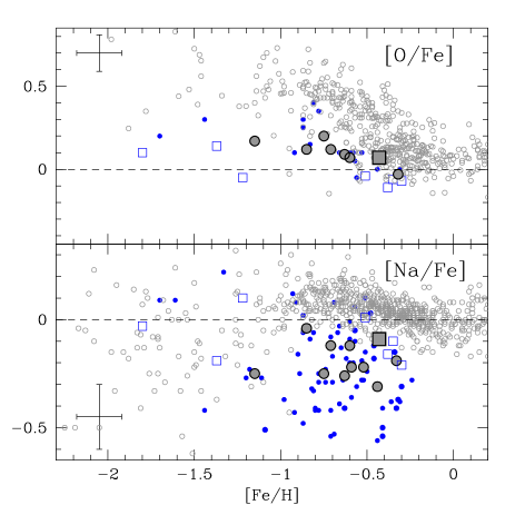
Figure 4: Behaviour of [O/Fe] (upper panel) and [Na/Fe] (lower panel) as a function of [Fe/H] for the observed stars: the grey square is the average value for the stars of NGC 1866, large grey points the individual LMC field stars, blue squares the intermediate-age LMC clusters by Mucciarelli et al. (2008b) and the old LMC clusters by Johnson et al. (2006) and Mucciarelli et al. (2010), the small grey points Galactic stars by Edvardsson et al. (1993); Fulbright (2000); Burris et al. (2000); Reddy et al. (2003); Gratton et al. (2003); Reddy et al. (2006) and the small blue points the LMC field giants by Pompeia et al. (2008) and Smith et al. (2002). Errorbars indicate the typical uncertainties arising from the atmospheric parameters and the error in the fitting procedure.

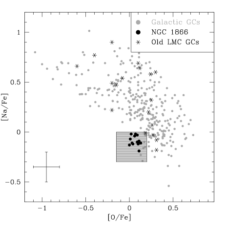
Figure 5: Behaviour of [Na/Fe] ratio as a function of [O/Fe] for the individual stars of NGC 1866 (black points). In comparison the individual stars observed in Galactic GCs (grey points) and in the old LMC GCs (black asterisks, by Mucciarelli et al., 2010) have been plotted. Light grey area indicates the mean locus defined by the stars measured by Mucciarelli et al. (2008b) in 4 intermediate-age LMC clusters

.

6.3 $\alpha$-elements

For the other $\alpha$-elements (namely, Mg, Si, Ca and Ti) NGC 1866 displays solar-scaled patterns, in a similar fashion of the field giants. Fig. 6 shows $<$$\alpha$/Fe$>$ (defined as mean of [Mg/Fe], [Si/Fe], [Ca/Fe] and [Ti/Fe]) as a function of [Fe/H]: a mild trend with the metallicity seems to be observed. $<$$\alpha$/Fe$>$ ratios in both NGC 1866 and the LMC field stars appear to be lower than those observed in the Galactic stars at the same metallicity level; the same result has been pointed out by Pompeia et al. (2008). At lower metallicities ([Fe/H]$<$–1 dex) the comparison between the LMC and the Galaxy is quite complex. In fact, the old LMC clusters by Mucciarelli et al. (2010) exhibit a quite good agreement with the Galactic Halo stars, while the clusters analyzed by Johnson et al. (2006) show systematically lower [Ti/Fe] and [Ca/Fe] ratios, but similar [Si/Fe] ratios. Note that the sample of LMC field stars discussed here does not include stars with [Fe/H]$<$-1.5 dex and does not allow to identify possible discrepancy between the [$\alpha$/Fe] ratio between the Halo stars and the metal-poor component of the LMC.

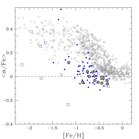
Figure 6: Behaviour of the [$\alpha$/Fe] ratio (defined as [Mg+Si+Ca+Ti/Fe]/4) as a function of [Fe/H]. Same symbols of Fig. 4.

6.4 Mn, Cu and Ni

Both [Mn/Fe] and [Cu/Fe] abundance ratios in our sample display significant underabundances with respect to the Galactic patterns (see Fig. 7). We found for NGC 1866 average values of [Mn/Fe]= –0.61 dex ($\sigma$= 0.08 dex) and [Cu/Fe]= –0.69 dex ($\sigma$= 0.07 dex). Such a depletion has been detected also in the LMC field stars that exhibit a clear trend of decreasing [Mn/Fe] and [Cu/Fe] with the metallicity. Ni abundances are [Ni/Fe]= –0.10 ($\sigma$= 0.08 dex) and [Ni/Fe]= –0.08 ($\sigma$= 0.08 dex) for cluster and field stars respectively.

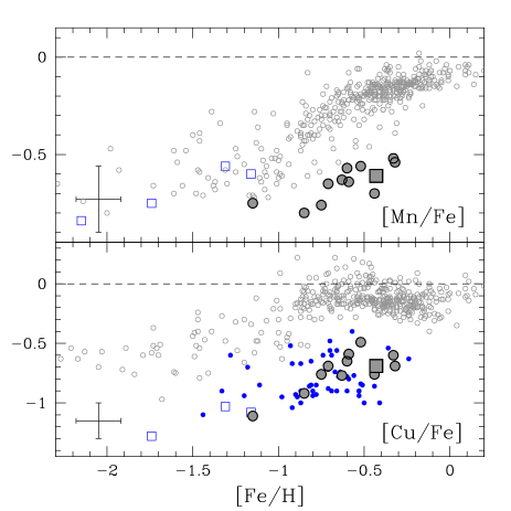
Figure 7: Behaviour of the [Mn/Fe] (upper panel) and [Cu/Fe] (lower panel) as a function of [Fe/H]. Same symbols of Fig. 4.

6.5 Neutron-capture elements

The elements belonging to the first peak of the s-elements, as Y and Zr, turn out to be depleted with respect to the solar value (Fig. 8): we found for NGC 1866 average values of [Y/Fe]= –0.40 dex ($\sigma$= 0.08 dex) and [Zr/Fe]= –0.41 dex ($\sigma$=0.09 dex), that well resemble the observed patterns in the field stars. On the other hand, we detected enhanced abundance ratios for the second s-peak elements Ba, La, Ce and Nd (see Fig. 9). We note a general offset between our abundances of [Zr/Fe] and [La/Fe] and the abundances by Pompeia et al. (2008), while for [Y/Fe] and [Ba/Fe] the two samples well agree. The origin of the discrepancy is likely due to the use of different transitions between the two works. Each GIRAFFE setup covers only a rather small wavelength coverage and we have observed different GIRAFFE setups than Pompeia et al. (2008). The use of different lines may bring some systematic offset in the retrieved abundances. This is usually averaged out by using many transitions, but residual differences may be present for those elements for which few transitions are available.

Abundances of other elements (namely Mo, Ru, Pr, Eu, Er, Hf and W) have been measured only for the star #2981 (see Tab. LABEL:cl), due to the large wavelength coverage of UVES. In particular, europium shows an enhanced value of [Eu/Fe]= +0.49 dex.

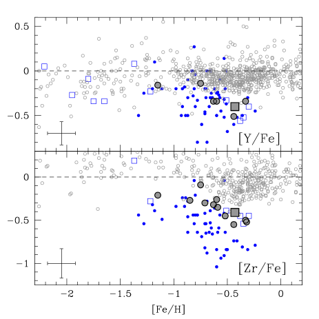
Figure 8: Behaviour of the [Y/Fe] (upper panel) and [Zr/Fe] (lower panel) as a function of [Fe/H]. Same symbols of Fig. 4.

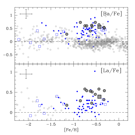
Figure 9: Behaviour of the [Ba/Fe] (upper panel) and [La/Fe] (lower panel) as a function of [Fe/H]. Same symbols of Fig. 4.

Table 6: Average abundance ratios for NGC 1866 and corresponding standard deviation.

Ratio	Average	$\sigma$
	(dex)	(dex)
$[Fe/H]$	–0.43	0.04
$[Na/Fe]$	–0.09	0.05
$[O/Fe]$	0.07	0.04
$[Mg/Fe]$	–0.05	0.08
$[Si/Fe]$	0.04	0.07
$[Ca/Fe]$	–0.02	0.10
$[Ti/Fe]$	–0.01	0.10
$[Mn/Fe]$	–0.61	0.08
$[Ni/Fe]$	–0.10	0.08
$[Cu/Fe]$	–0.69	0.07
$[Y/Fe]$	–0.40	0.08
$[Zr/Fe]$	–0.41	0.09
$[Ba/Fe]$	0.56	0.06
$[La/Fe]$	0.39	0.15
$[Ce/Fe]$	0.29	0.11
$[Nd/Fe]$	0.37	0.10

7 Discussion

The Star Formation History (SFH) of irregular galaxies like the LMC is deeply different from the Milky Way; it is thought to develop slowly, with several, short bursts of star formation, followed by long quiescent periods. The theoretical interpretation of the chemical patterns in stars belonging to LMC requires therefore some important caveats; in particular, we stress the role that dynamical environmental processes (such as tidal interaction and/or ram pressure stripping) may have on the chemical evolution of a galaxy (see, e.g., Bekki (2009) and references therein). Indeed, Besla et al. (2007) have suggested that the LMC entered the Galactic virial radius $\sim$3 Gyr ago, and tidal interactions with the Galaxy and the Small Magellanic Cloud likely triggered star formation that appears to have lasted $\sim$1 Gyr following that event. In our analysis we do not account for such effects.
As it is well known, main classes of chemical polluters are:

• SuperNovae of type Ia (SN Ia), responsible for a large production of iron and iron-peak elements;

• SuperNovae of type II (SN II), which synthesize oxygen, $\alpha$ elements, iron and iron-peak elements, elements belonging to the weak component of the s-process and the r-process elements;

• asymptotic giant branch (AGB) stars, which pollute the Interstellar Medium (ISM) with carbon and elements belonging to the main component of the s-process.

At the moment, the exact stellar site in which the r-process takes place is still a matter of debate: this fact leads to strongly different nucleosynthetic paths depending on the adopted physics and theoretical assumptions (Qian & Wasserburg, 2007; Kratz et al., 2007). More robust theoretical predictions are available for the s-process (Gallino et al., 1998; Busso, Gallino & Wasserburg, 1999; Cristallo et al., 2009), which characterizes the thermally pulsing phase of low mass AGB stars (TP-AGB phase).

In the following, we discuss three main aspects of our results: (i) the internal abundance scatter of the stars in NGC 1866, in light of the self-enrichment scenario invoked to explain the internal abundance spread of the old GCs; (ii) possible chemical variations due to the different evolutive stages of the observed stars in this work; (iii) the chemical abundances of NGC 1866 and its surrounding field in light of the chemical evolution of the LMC.

7.1 NGC 1866 internal abundance scatter

Before analyzing the spectroscopic patterns of single stars belonging to the cluster, it is useful to compare abundances of cluster stars with respect to stars lying in the surrounding field. From Fig. 3, in which we report mean values for NGC 1866 and for the field, it clearly emerges that the two groups present very similar spectroscopic patterns, showing values consistent within the error bars.

As far as the light element are concerned (O, Na, Al, Mg), this pattern is quite different from what observed in globular cluster stars (see e.g. the review by Gratton, Sneden & Carretta, 2004) which show two distinctive aspects: (i) the first is that GC stars show a large spread in these light elements, indicating inhomogeneous pollution of H burning rich material, and (ii) the second that, because of these effect, the average abundances of GC stars are different from those of the field stars with similar metallicity.

We shall emphasize that the chemical abundances of NGC 1866 do not show any evidence for these effects: we do not observe appreciable chemical spread within the cluster and the abundances of NGC 1866 are in very good agreement with those of the LMC field.

Self-pollution within the cluster, as originated for example by intermediate AGB stars (e.g. Ventura & D’Antona 2009), cannot be completely excluded because of the limited number of stars within our sample. However we note that in most Galactic GCs observed with high resolution spectroscopy the percentage of ’polluted’ stars is significant, at least $\sim$50% of the entire population (see e.g. Carretta et al., 2009) and we should expect some clear detection within our stars sample. As shown in Fig. 5 the stars of NGC 1866 well overlap the mean locus defined by the giants discussed in Mucciarelli et al. (2008b), with solar or mild sub-solar [O/Fe] ratios and sub-solar [Na/Fe] ratios. This finding, combined with the good agreement between cluster and field stars abundance ratios, seems to confirm that all these stars belong to the first (unpolluted) generation of the clusters, while there are no hints of polluted stars . The lack of anti-correlations in NGC 1866, as far as in the intermediate-age, massive LMC clusters, suggests that the younger LMC GCs do not undergo the self-enrichment process, following different formation and evolution processes with respect to the old stellar clusters (in both Milky Way and the LMC).

Recently, Carretta et al. (2010) propose to define GCs as those stellar clusters where a Na-O anticorrelation is observed. This new definition has the appealing advantage to provide an easy boundary to separate GCs and other loose stellar systems (as the open clusters). We stress that this is a local definition based only on the Milky Way stellar clusters, where there is clear separation in age and mass between open and globular clusters, and there is a lack of massive, young stellar clusters (at variance with the LMC). According to this new definition, NGC 1866 (and all the intermediate-age LMC clusters so far observed) would not be classified as a globular cluster. However, these objects appear to be structurally different and more massive than the typical mass ($<10^{4}M_{\odot}$) of the open clusters. Thus, the young populous globular-like clusters in the LMC seem to be a class of objects intermediate between open clusters and true (old) globular clusters.

The main question arising from these findings is to understand why these young LMC massive clusters do not suffer the self-enrichment process. Previous investigations of old GCs show that several parameters (e.g. mass, metallicity, orbital parameters) may influence the amount of the self-enrichment process. We note that the most metal-rich Galactic clusters (with overall metallicities comparable to NGC 1866) are more massive than NGC 1866 by one order of magnitude and thus in the Milky Way there are no clusters similar to NGC 1866 in the mass/metallicity plane.

The chemical homogeneity of NGC 1866 is very important because it demonstrates that the chemical inhomogeneities observed in the old GC stars are peculiar to these objects. NGC 1866 is only a few times less massive than NGC 6397 and M 4 where inhomogeneities have been observed, so it does not seem likely that mass alone can be the cause of the differences and other causes should be invoked, such as, for instance, the fast time formation of the GC and the (in)homogeneity of the early ISM.

However, a point to recall is that the young LMC clusters share with several old GCs the same present-day mass but probably not the same initial mass. In fact, dynamical simulations (D’Ercole et al., 2008, 2010) suggest that a large fraction of the first stellar generation is lost in the early evolution of the cluster and thus the initial mass of the cluster was one-two order of magnitude higher than the present-day mass. These findings suggest that GCs born with initial mass of the order of $\sim 10^{5}M_{\odot}$ (similar to the mass of the LMC clusters younger than $\sim$2 Gyr) are not massive enough to retain their pristine gas and undergo the self-enrichment process.

7.2 NGC 1866 and evolutive, chemical changes

Since chemical abundance variations can be produced in evolved stars by several processes occurring during the stellar evolution, as a further step we analyzed the evolutionary status of stars in our sample, in order to determine whether we could find surface chemical variations due to events that occurred in their previous evolution.

The majority of the target stars within our sample lie on their RGB and Blue Loop stages and also a few of stars (the brightest and reddest ones) belong to the AGB phase. Therefore, the majority of stars belonging to our sample have experienced a unique dredge up event, the so-called First Dredge Up (FDU). Stars belonging to NGC 1866 that evolve off of their Main Sequence phase have a mass of about $M=4.5M_{\odot}$ (according to the evolving mass of the cluster as found by Brocato et al. 2003). Before their first ascent along the Giant Branch, stellar theory predicts that, in these stars, the FDU causes a strong depletion of ¹²C ($-40$% $\div-30$%), a noticeable enrichment of the surface nitrogen (a factor 2) and a minor decrease of the oxygen surface abundance. Unfortunately we could only determine the surface oxygen abundance and, therefore, we cannot clearly identify the signature of FDU in our stars. We focus our attention on the most evolved object in our sample (the star labelled #2981) for which we can have a large number of elements (due to the large spectral coverage provided from UVES). There are other two stars (namely, #2131 and #5231) that likely belong to the Early-AGB stage, but they are $\sim$200 K hotter than #2981 and some elements cannot be measured due to the GIRAFFE spectral coverage. Thus, these two stars are not ideal to identify evolutive, chemical changes.
In order to identify its precise evolutionary phase, we computed a model of a star with initial mass $M=4.5M_{\odot}$ and $Z=6\times 10^{-3}$ by means of a recent version of the FRANEC stellar evolutionary code (Chieffi et al., 1998; Straniero et al., 2006; Cristallo et al., 2009). In Fig. 10 we compare the surface gravity and temperature of the model (blue curve) with data relative to #2981 (red triangle). The comparison shows that this star has not yet reached its TP-AGB phase or, at least, it just suffered for a few TPs. The structure of an AGB star consists of a partial degenerate C-O core, an He-shell, an H-shell and a convective envelope. The hydrogen burning shell, which provides the energy necessary to sustain the stellar luminosity, is regularly switched off by the growth of thermal runaways (Thermal Pulses, TPs). These episodes, driven by violent He ignitions within the He buffer (He-intershell), cause this region to become dynamically unstable against convection for short periods: once convection quenches off within the He-intershell, a period of quiet He-burning follows, during which the convective envelope can penetrate in the underlying layers (this phenomenon is known as Third Dredge Up, TDU), carrying to the surface the freshly synthesized carbon and s-process elements. If the star #2981 would had already suffered a consistent number of TDU episodes, we would expect noticeable changes in its s-process surface abundances. A comparison between its spectroscopic data and the median overabundances of the cluster shows consistent values within error-bars (see Fig. 11), therefore supporting the hypothesis that this star is still on its Early-AGB phase. Unfortunately, spectral lines of some key light elements (lithium, carbon and nitrogen) are not contained in the observed spectral range. The abundance of these elements would provide more stringent chemical constraints on the evolutionary phase of #2981, owing to the occurrence of the already described TDU episodes or to the presence of other physical processes, such as the Hot Bottom Burning (HBB) (see, for example, the analysis presented by McSaveney et al. (2007) on their AGB star labeled NGC 1866#4).

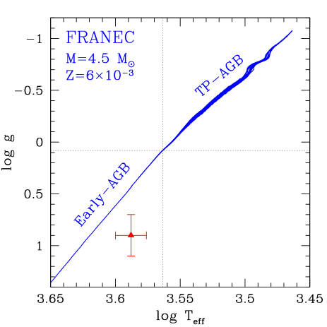
Figure 10: Theoretical surface gravity and temperature (blue line) compared with data relative to #2981. See text for details.

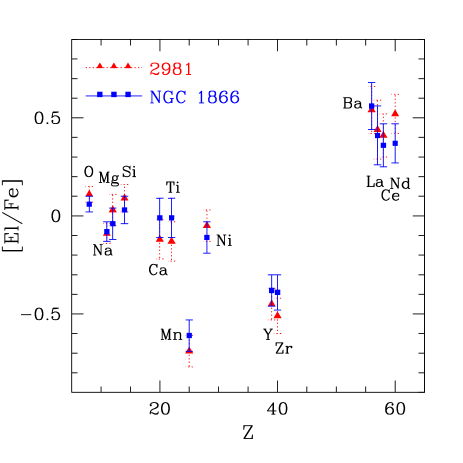
Figure 11: Comparison between the spectroscopic values of the cluster star labelled #2981 (red triangles) and the median of stars belonging to the cluster (blue squares).

7.3 The chemical evolution of the LMC

Our analysis excludes that the spectroscopic patterns observed in NGC 1866 derive from the evolutionary phase of the observed stars or from the internal evolution of the cluster: a wider analysis, which spans over the entire evolutionary history of the LMC, is therefore necessary. Such an analysis relies on many physical inputs, the most important being the SFH and the stellar yields. We just remind that, in the LMC, a rapid chemical enrichment occurred at a very early epoch, followed by a long period with reduced star formation and, most recently (about 3 Gyr ago), by another period of chemical enrichment (see e.g. Bekki & Chiba, 2005).
Concerning the stellar yields, in order to reproduce the heavy elements ($Z>35$) observed spectroscopic patterns with theoretical models, we need to hypothesize that two classes of stellar objects polluted the ISM before the formation of NGC 1866: massive stars, which synthesized the r-process elements (such as, for example, europium) and the weak component of the s-process, and AGB stars, which produced the elements belonging to the main component of the s-process. In Fig. 12 we compare our theoretical expectations with spectroscopic data of #2981 since, for this star, we have high resolution spectra and a more complete element line list at our disposal. Note that some of the abundance ratios discussed in the follows are based on one only star (see Table LABEL:cl). A conservative errorbar of 0.2 dex has been adopted for each element.

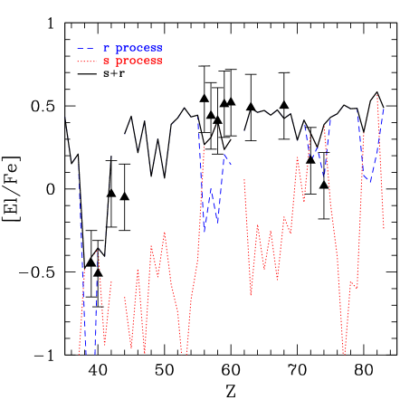
Figure 12: Comparison between the spectroscopic values of #2981 (black triangle) and the expected theoretical trend (dark solid line). The single contributions from the s-process and the r-process are represented by the red dotted line and the blue dashed line, respectively. See text for details.

As already discussed, theoretical r-process distributions still suffer from major uncertainties, such as the identification of the stellar site or the determination of the precise relative abundance patterns. For this reason, the r-process contribution to the solar distribution is usually calculated based on the solar s-process contribution, following the formula $r=1-s$ (see, e.g., Arlandini et al. 1999). Then, a generic r-process distribution at a fixed metallicity can be obtained by normalizing the distribution to a single r-only element (or to an element whose production is almost totally ascribed to the r-process) and by adopting the solar elemental ratios for the other elements. We tentatively apply this procedure, which works well for the Milky Way (see, e.g., Sneden et al. 2008), to NGC 1866. In order to determine the r-process enrichment level we focus on europium. We know that about 95% of its Galactic abundance can be ascribed to the r-process and we assume that the same should occur in the Magellanic Clouds. We fix the europium overabundance to the value of #2981, ([Eu/Fe]$\sim$0.49). Then, we derive the r-process pattern by adopting the elemental r-process solar percentages tabulated in Bisterzo et al. (2009). In Fig. 12, the r-process contribution is highlighted with a blue dotted line.
The s-process contribution has been calculated by means of the FRANEC code, in which we couple a complete nuclear network (able to follow in detail the whole s-process nucleosynthesis) directly to the physical evolution of the model (Cristallo et al., 2009). We run, as a representative mass of AGB pollution, a 2 $M_{\odot}$ model with $Z=3\times 10^{-3}$ and we hypothesize that the present-day observed s-process patterns result from the pollution due to a single generation of low mass AGB stars. This assumption is justified by the relatively fast chemical evolution of LMC up to [Fe/H]$\sim$–1 (see e.g. Bekki & Chiba, 2005). Then, we applied a dilution to the theoretical curve in order to match the cerium abundance (red dotted curve in Fig. 12): this dilution mimic the fact that the mass lost by AGB stars has been mixed with s-process free material from which originate the present-day observed stars.
The final theoretical distribution (dark solid curve) results from the sum of the s-process and the r-process contributions. The agreement with spectroscopic data is quite good, proving the validity of our theoretical scheme and validating the assumption made in the determination of the r-distribution of our sample (thus possibly evidencing a sort of universality of the r-process). Unfortunately, the current set of spectroscopic abundances can not lead us in precisely identifying the metallicity of AGB population which previously polluted the ISM. In Fig. 13, we show different theoretical chemical patterns (including the r-component) obtained with AGB models of different metallicities (red dotted line for $Z=6\times 10^{-3}$, dark solid line for $Z=3\times 10^{-3}$ (our reference model), blue dashed line for $Z=1\times 10^{-3}$ and magenta dot-dashed line for $Z=1\times 10^{-4}$). Note that, depending on the metallicity, theoretical models present different enrichment level; before comparing them, we therefore normalize distributions to the cerium abundance in order to highlight the relative variations in the s-process shape. We only highlight the elements, within our sample, which receive a consistent contribution ($>$50%) from the s-process: within error-bars, our spectroscopic data do not permit us to clearly discriminate between the three distributions. In order to do that we would need to observe lead, at the termination of the s-process path, since the abundance of this element is extremely sensitive to the metallicity. In fact, the lower the metallicity, the more efficient the Pb production is (see, e.g., Bisterzo et al. 2009): ranging from $Z=1\times 10^{-4}$ to $Z=6\times 10^{-3}$ a difference of more than a factor 20 (1.3 dex) is expected.

Figure 13: Theoretical chemical patterns obtained with AGB models at different metallicities. See text for details.

Actually, Reyniers et al. (2007) determined the spectroscopic abundances of elements belonging to the three peaks of the s-process (included lead in a LMC post-AGB star (MACHO 47.2496.8). When looking to the relative distribution, it turns out that the observed path agrees well with our reference model, whose lead overabundance is comparable to the ones characterizing the hs elements. However, more statistics are needed before claiming any definitive chemical evolutionary theory.

How do our conclusions fit into a more global view of the LMC chemical evolution? In order to answer to this complex question we need to compare our data with other LMC samples and to extend our analysis to abundances of light elements, iron-peak elements and copper.
Concerning heavy elements abundances, stars belonging to LMC present noticeable differences with respect to their Galactic counterparts (see Fig. 8 and Fig. 9). In fact, while in Galactic stars the light elements and heavy elements distributions are nearly flat (showing values around 0), in LMC they present dichotomic trends.
Let us start from the heavy s-process (hs) elements. In 2006, Johnson et al. (2006) performed a spectroscopic analysis on 10 red giants belonging to four old LMC GCs. Apart from the most metal-poor GC (Hodge 11), which shows no enhancements at all, in other clusters a mild enhancement of hs elements ([hs/Fe]$\sim$0.3 dex) has been found. Similarly, the study of 27 giants belonging to four intermediate-age LMC GCs by Mucciarelli et al. (2008a) evidenced a smooth enhancement of heavy elements, consistent with that found in old LMC GCs. This trend, which also characterizes metal-poor red giants belonging to dwarf spheroidal galaxies (dSph) (Shetrone et al., 2003; Venn et al., 2004), can be easily ascribed to a different SFH of the hosting galaxy. In the LMC, the slower temporal increase of iron with respect to the Milky Way makes the contribution from metal-poor AGB stars more important at a given time or metallicity. Since these objects produce more heavy elements than light elements, a rise of the heavy elements component has to be expected (and it is actually observed). Stars belonging to NCG 1866, which formed only $10^{8}$ years ago, perfectly match the mild enhancement observed in others GCs (see Fig. 9). As stressed above, in order to determine the metallicity of this class of AGB polluters, the spectroscopic determination of lead is required.
Oppositely to hs elements, light s-process (ls) elements show a decreasing curve with respect to Galactic stars at large metallicities. This trend is fully confirmed by our sample. A similar behaviour has also been observed in dSph’s (Venn et al., 2004; Shetrone et al., 2003): beneath various theoretical recipes, these authors proposed that these underabundances with respect to the MW could be ascribed to a reduced contribution from metal-rich AGB stars or to metallicity dependent yields from SN II (Timmes et al., 1995). Both hypotheses are strictly correlated to the peculiar chemical enrichment that the hosting galaxy experimented in the past. In LMC, the long gap between the two star formation bursts has played a fundamental role, melting the contributions from massive stars and SNIa in a different way with respect to the MW. A strong reduction in the SFR could have heavily reduced the contribution from AGB stars of intermediate metallicities, causing in such a way a decrease of the light elements (note that the yields of light elements from low mass AGB stars grow with the metallicity). On the other hand, the behaviour of other elements efficiently produced by massive stars ($\alpha$ elements, Na, Mn and Cu) present, at a fixed metallicity, lower overabundances with respect to the MW (see Figures 4, 6 and 7), suggesting de facto a reduced contribution from massive stars with respect to SN Ia. This statement is however contrasted by the nearly flat europium distribution observed in LMC stars ([Eu/Fe]$\sim$0.5) at all metallicities (up to [Fe/H]$\sim--0.3$). We therefore conclude that a theoretical analysis based on stellar yields only cannot lead to a clear explanation for the ls elements distribution in stars belong to the LMC. Under this perspective, physical mechanisms involving the whole LMC structure have to be considered, such for example dynamical environmental processes (Bekki, 2009) or the presence of Galactic winds (Lanfranchi et al., 2008).

8 Conclusions

In this paper, we have studied the chemical abundances of 25 stars in the field of the LMC star cluster NGC 1866. The accurate analysis and the high efficiency of FLAMES@VLT allows us to obtain a set of high quality measurements of the abundances of this region of the LMC. We emphasize that we do not observe significant element by element abundance spread amongst the NGC 1866 stars, and we find that the cluster chemical pattern fits very well with the general pattern observed in the LMC field stars. We note that this is in stark contrast with what is observed with Galactic globular clusters and our result, if confirmed on a larger sample of stars, would bring insight to the debate of the formation mechanisms for globular clusters in general.

The main observational results are summarized as follows:

1. The average iron abundance of NGC 1866 is [Fe/H]= –0.43$\pm$0.01 dex ($\sigma$= 0.04 dex).

2. [O/Fe]= 0.07 ($\sigma$= 0.04 dex) and [Na/Fe]=-0.09 ($\sigma$= 0.05 dex )abundance ratios appear to be lower than those measured in Galactic stars and the O/Na values are, within the uncertainties, very similar between different stars in NGC 1866.

3. The lack of anti-correlations suggests that NGC 1866 does not undergo the self-enrichment process at variance with the old GCs in both Milky Way and LMC. Similar results have been found in the intermediate-age LMC clusters, suggesting that GCs formed with an initial mass of the order of $\sim 10^{5}M_{\odot}$ are not massive enough to retain their pristine gas. Also, other possible effects (i.e. a mass/metallicity threshold, inhomogeneity of the early ISM, tidal effects due to the interactions with the SMC and the Milky Way) cannot be ruled out, playing a role to inhibit the self-enrichment process.

4. $\alpha$-elements in the cluster and in the field stars show a solar-scaled behaviour. Also $<\alpha/Fe>$ is measured lower than that found in the Galaxy.

5. With respect to the Galaxy, a depletion in the abundances of [Mn/Fe] and [Cu/Fe] is found both in field and cluster stars. A value of [Ni/Fe] $\simeq$–0.10 dex is also measured.

6. Abundances of neutron-capture elements are derived: in the case of Y and Zr values lower than the solar ones are measured, while [Ba/Fe], [La/Fe], [Ce/Fe] and [Nd/Fe] ratios appear to be enhanced. The UVES measurement of a single NGC 1866 star shows a value of [Eu/Fe] $\simeq$ +0.49 dex.

With this observational framework we applied modern stellar evolution theory and nucleosynthesis calculations to make three major conclusions. We do caution, however, that our data apply only to a single region of the LMC and that abundances of several key elements are lacking, and we hope that our work will stimulate further investigations, both observational and theoretical. Notwithstanding, the following considerations can be emphasized:

(i)  The very similar pattern found for the abundances of both field and cluster stars suggests that stars belonging to NGC 1866 originate from pollution episodes that occurred before the formation of the cluster. Nevertheless, self-enrichment between cluster stars cannot be completely ruled out because of the small number of stars.

(ii)  Surface chemical variations in evolved stars (core He burning and early AGB phases) due to events that occurred in their previous evolution cannot be recognized from data presented in this work. Further observations of light elements are recommended to derive more robust constraints.

(iii) From a relatively simple model we show that the observed abundances of heavy elements (Z $>$ 35) can be reproduced by the sum of s-process and r-process contributions as expected by pollution mechanisms due to i) massive stars and ii) single generation of low mass AGB stars. However, the result obtained in this work suggest a further theoretical effort to properly understand the evolution of s-process elements (in particular the ls ones) in the context of the LMC chemical evolution. Moreover, precise spectroscopic measurements of lead are suggested to provide indication on the metallicity of the low mass AGB stars which could be significant contributors to the observed abundances of s-process elements in LMC stars.

Part of this work has been supported by the Spanish Ministry of Science and Innovation projects AYA2008-04211-C02-02. The authors warmly thank the anonymous referee for his/her suggestions in improving the paper and Vanessa Hill for her comments and suggestions. A.M. thanks the Observatoire de Meudon, Paris, for its hospitality during the early stage of this work. S.C. thanks Carlos Abia and Roberto Gallino for stimulating discussions

References

- Alonso et al. (1998) Alonso, A., Arribas, S., & Martinez-Roger, C., 1998, A&As, 131, 209
- Alonso et al. (1999) Alonso, A., Arribas, S., & Martinez-Roger, C., 1999, A&As, 140, 261
- Arlandini et al. (1999) Arlandini, C., Käppeler, F., Wisshak, K., Gallino, R., Lugaro, M., Busso, M., & Straniero, O., 1999, ApJ, 525, 886
- Bekki & Chiba (2005) Bekki, K., & Chiba, M., 2005, MNRAS, 356, 680
- Bekki (2009) Bekki, K., 2009, IAU Symp. 256, 105
- Besla et al. (2007) Besla, G. et al., 2007, ApJ, 668, 949
- Bisterzo et al. (2009) Bisterzo, S., Gallino, R., Straniero, O., Cristallo, S. & Kappeler, F. 2010, MNRAS, 404, 1529
- Brocato et al. (2003) Brocato, E., Castellani, V., Di Carlo, E., Raimondo, G., & Walker, A. R., 2003, AJ, 125, 3111
- Burris et al. (2000) Burris, D. L., Pilachowski, C. A., Armandroff, T. E., Sneden, C., Cowan, J. J., & Roe, H., 2000, ApJ, 544, 302
- Busso, Gallino & Wasserburg (1999) Busso, M., Gallino, R., & Wasserburg, G. J., 1999, ARA&A, 37, 239
- Caffau et al. (2005) Caffau, E., Bonifacio, P., Faraggiana, R., Francois, P. Gratton, R. G., & Barbieri, M., 2005, A&A, 441, 533
- Caffau et al. (2008) Caffau, E., Ludwig, H.-G., Steffen, M., Ayres, T. R., Bonifacio, P., Cayrel, R., Freytag, B., & Plez, B., 2008, A&A, 488, 1031
- Carpenter (2001) Carpenter, J. M., 2001, AJ, 121, 2851
- Carretta et al. (2009) Carretta, E. et al., 2009, A&A, 505, 117
- Carretta et al. (2010) Carretta, E. et al., 2010, A&A, 516, 55
- Castelli & Kurucz (2003) Castelli, F., & Kurucz, R. L., 2003, in IAU Symposium, Ed. N. Piskunov, W. W. Weiss & D. F. Gray, 20P
- Cayrel et al. (1999) Cayrel, R., Spite, M., Spite, F., Vangioni-Flam, E., Cassé, M. & Audouze, J., 1999, A&A, 343, 923
- Chieffi et al. (1998) Chieffi, A., Limongi, M., & Straniero, O., 1998, ApJ, 502, 737
- Cole et al. (2005) Cole, A. A., Tolstoy, E., Gallagher, J. S., III, & Smecker-Hane, T. A., 2005, AJ, 129, 1465
- Colucci, Bernstein and McWilliam (2010) Colucci, J.E., Bernstein, R. A., & McWilliam, A., 2010, arXiv:1009.4195v1
- Cristallo et al. (2009) Cristallo, S., Straniero, O., Gallino, R., Piersanti, L., Domínguez, I. & Lederer, M.T., 2009, ApJ, 696, 797
- Cunha et al. (2002) Cunha, K., Smith, V. V., Suntzeff, N. B., Norris, J. E., Da Costa, G. S., & Plez, B., 2002, AJ, 124, 379
- Den Hartog et al. (2003) Den Hartog, E. A., Lawler, J. E., Sneden, C., & Cowan, J.J., 2003, ApJS, 148, 543
- D’Ercole et al. (2008) D’Ercole, A., Vesperini, E., D’Antona, F., McMillan, S. L. W., & Recchi, S., 2008, MNRAS, 391, 825
- D’Ercole et al. (2010) D’Ercole, A., D’Antona, F., Ventura, P., Vesperini, E., & McMillan, S. L. W., 2010, MNRAS, 407, 854
- Edvardsson et al. (1993) Edvardsson, B., Andersen, J., Gustafsson, B., Lambert, D. L., Nissen, P. E., & Tomkin, J., 1993, A&A, 275, 101
- Fulbright (2000) Fulbright, J. P., 2000, AJ, 120, 1841
- Gallino et al. (1998) Gallino, R., Arlandini, C., Busso, M., Lugaro, M., Travaglio, C, Straniero, O., Chieffi, A. & Limongi, M., 1998,ApJ, 497, 388
- Gratton et al. (1999) Gratton, R. G., Carretta, E., Eriksson, K., & Gustafsson, B., 1999, A&A, 350, 955
- Gratton et al. (2003) Gratton, R. G., Carretta, E., Claudi, R., Lucatello, S., & Barbieri, M., 2003, A&A, 404, 187
- Gratton, Sneden & Carretta (2004) Gratton, R. G., Sneden, C. & Carretta, E., 2004, ARA&A, 42, 385
- Grevesse & Sauval (1998) Grevesse, N., & Sauval, A. J., 1998, SSRv, 85, 161
- James (1998) James, F., 1998, MINUIT, Reference Manual, Version 94.1, CERN, Geneva, Switzerland
- Johansson et al. (2003) Johansson, S, Litzen, U., Lundberg, H., & Zhang, Z., 2003, ApJ, 584, 107L
- Johnson et al. (2006) Johnson, A.J., Ivans, I.I., & Stetson, P.B., 2006, ApJ, 640, 801
- Harris & Zaritsky (2009) Harris, J., & Zaritsky, D., 2009, AJ, 138, 1243
- Hill et al. (2000) Hill, V., Francois, P., Spite, M., Primas, F., & Spite, F., 2000, A&As, 364, 19
- Hodge (1960) Hodge, P. W., 1960, ApJ , 131, 351
- Hodge (1961) Hodge, P. W., 1961, ApJ , 133, 413
- Kratz et al. (2007) Kratz, K.-L., Farouqi, K., Pfeiffer, B., Truran, J.W., Sneden, C., Cowan, J.J., 2007, ApJ, 662, 39
- Kurucz (1993a) Kurucz, R. L., 1993a, ATLAS9 Stellar Atmosphere Programs and 2 km/s grid. Kurucz CD-ROM No. 13. Cambridge, Mass,: Smithsonian Astrophysical Observatory, 1993., 13
- Kurucz (1993b) Kurucz, R. L., 1993b, SYNTHE Spectral Synthesis Programs and Line Data. Kurucz CD-ROM No. 18. Cambridge, Mass,: Smithsonian Astrophysical Observatory, 1993., 18
- Lanfranchi et al. (2008) Lanfranchi, G.A., Matteucci, F., & Cescutti, G., 2008, A&A, 481, 635
- Lawler et al. (2001a) Lawler, J. E., Wickliffe, M. E., den Hartog, E. A., & Sneden, C., 2001, ApJ, 563, 1075
- Lawler et al. (2001b) Lawler, J. E., Bonvallet, G., & Sneden, C., 2001, ApJ, 556, 452
- Lodders, Palme & Gail (2009) Lodders, K., Palme, H., & Gail, H.-P., 2009, arXiv0901.1149L
- Magain (1984) Magain, P. 1984, A&A, 134, 189
- Matteucci & Brocato (1990) Matteucci, F., & Brocato, E., 1990, ApJ, 365, 539
- McSaveney et al. (2007) McSaveney, J.A., Wood, P.R., Scholz, M., Lattanzio, J.C., & Hinkle, K.H., 2007, MNRAS, 378, 1089
- Mucciarelli et al. (2006) Mucciarelli, A., Origlia, L., Ferraro, F. R., Testa, V., & Maraston, C., 2006, ApJ, 646, 939
- Mucciarelli et al. (2008a) Mucciarelli, A., Caffau, E., Freytag, B., Ludwig, H.-G., & Bonifacio, P., 2008, A&A, 484, 841
- Mucciarelli et al. (2008b) Mucciarelli, A., Carretta, E., Origlia, L. & Ferraro, F. R., 2008, AJ, 136, 375
- Mucciarelli et al. (2009) Mucciarelli, A., Origlia, L., Ferraro, F. R., & Pancino, E., 2009, ApJ, 695, 134L
- Mucciarelli et al. (2010) Mucciarelli, A., Origlia, L.& Ferraro, F. R.2010, ApJ, 717, 277
- Musella et al. (2006) Musella, I., Ripepi, V., Brocato, E., Castellani, V., Caputo, F., Del Principe, M., Marconi, M., Piersimoni, A. M., Raimondo, G., Stetson, P. B., & Walker, A. R., 2006, MemSaIt, 77, 291
- Pasquini et al. (2002) Pasquini, L. et al., 2002, Messenger, 110, 1
- Pompeia et al. (2005) Pompeia, L., Hill V. & Spite, M., 2005, NuPhA, 758, 242
- Pompeia et al. (2008) Pompeia, L., et al., 2008, A&A, 480, 379
- Prochaska et al. (2000) Prochaska, J. X., Naumov, S. O., Carney, B. W., McWilliam, A., & Wolfe, A., 2000, AJ, 120, 2513
- Qian & Wasserburg (2007) Qian, Y.-Z., & Wasserburg, G.J., 2007, PhR, 442, 237
- Reddy et al. (2003) Reddy, B. E., Tomkin, J., Lambert, D. L., & Allende Prieto, C., 2003, MNRAS, 340, 304
- Reddy et al. (2006) Reddy, B. E., Lambert, D. L., & Allende Prieto, C., 2006, MNRAS, 367, 1329
- Reyniers et al. (2007) M. Reyniers, C. Abia, H. Van Winckel, T. Lloyd Evans, L. Decin, K. Eriksson, & K. R. Pollard, 2007, A&A, 461, 641
- Rieke & Lebofsky (1985) Rieke, G. H., & Lebofsky, M. J., 1985, ApJ, 288, 618
- Sbordone et al. (2004) Sbordone, L., Bonifacio, P., Castelli, F., & Kurucz, R. L., 2004, MemSaIt, 5, 93
- Shetrone et al. (2003) Shetrone, M., Venn, K.A., Tolstoy, E., Primas, F., Hill, V., & Kaufer, A., 2003, AJ, 125, 684
- Smith et al. (2002) Smith, V.V., et al., 2002, AJ, 124, 3241
- Sneden et al. (2008) Sneden, C., Cowan, J.J., & Gallino, R., 2008, ARA&A, 46, 241
- Staveley-Smith et al. (2003) Staveley-Smith, L., Kim, S., Calabretta, M. R., Haynes, R. F., & Kesteven, M. J., 2003, MNRAS, 339,87
- Straniero et al. (2006) Straniero, O., Gallino, R., & Cristallo, S., 2006, Nucl. Phys. A, 777,311
- Storey & Zeippen (2000) Storey, P. J., & Zeippen, C. J., 2000, MNRAS, 312, 813
- Timmes et al. (1995) Timmes, F., Woosley, S.E., & Weaver, T.A., 1995, ApJS, 98, 617
- Tolstoy, Hill & Tosi (2009) Tolstoy, E., Hill, V., & Tosi, M., 2009, ARA&A, 47, 371
- van den Bergh & Hagen (1968) van den Bergh, S. & Hagen, G. L., 1968, AJ, 73, 569
- van den Bergh & de Boer (1984) van den Bergh, S. & de Boer, K. D., 1984, Structure and evolution of the Magellanic Clouds, Proceedings of the 108th IAU Symposium Dordrecht: Reidel 1984
- Venn et al. (2004) Venn, K. A., Irwin, M. Shetrone, M. D., Tout, C. A., Hill, V., & Tolstoy, E., 2004, AJ, 128, 1177
- Ventura & D’Antona (2009) Ventura, P., & D’Antona, F., 2009, A&A, 499, 835
- Wahlgren (2005) Wahlgren, G. M., 2005, MemSaIt Suppl., 8, 108
- Walker et al. (2001) Walker, A. R., Raimondo, G., Di Carlo, E., Brocato, E., Castellani, V., & Hill, V., 2001, ApJ, 560, 139L